Post Syndicated from Karsten Ploesser original https://aws.amazon.com/blogs/compute/scaling-rl-rollouts-with-firecracker-on-amazon-ec2-metal/
Modern reinforcement learning (RL) systems rely on thousands of rollout environments running in parallel. For large language model (LLM) training using Verifiable Rewards (RLVR) each rollout environment runs in a tightly isolated sandbox so state never leaks between environments.
The faster you can recycle sandboxes, the more training steps you can run per hour. That means higher rollout density per host which directly lowers your cost per step.
But density is a tuning knob with two failure modes. Push it too high and you hit a tail latency cliff. Play it too safe and you overprovision, leaving money on the table. The sweet spot depends on your instance type, workload profile, and how your training algorithm amplifies stragglers.
This post shows how to find that setting. We walk through the tunables that control density on Amazon EC2 metal. We then introduce labsweep, a measurement harness for mapping your latency and density curve. Throughout the post, we draw on lessons learned from production deployments with customers. The post is written for readers familiar with Kernel-based Virtual Machine (KVM), Firecracker, and container orchestration.
Background: EC2 metal, Nitro, and Firecracker
The AWS Nitro System offloads networking, storage, and security to dedicated hardware. Amazon EC2 instances expose a stable CPU topology you can inspect and pin workloads against. On Amazon EC2 metal, applications run directly on the underlying hardware.
Firecracker is a lightweight virtual machine monitor (VMM) designed for high density workloads. Each microVM boots quickly, runs its own Linux kernel, and has a small memory footprint.
Running Firecracker on Amazon EC2 metal combines direct access to underlying hardware with lightweight virtualization to support high density sandboxing. The key question is how far you can increase density before tail latency hurts the RL training loop.
Solution overview
The following diagram shows the reference architecture of a production RL sandbox node. This architecture serves as the foundation for the rest of the post. An Amazon EC2 metal instance runs a host agent that manages Firecracker microVMs, CPU pinning, non-uniform memory access (NUMA)-aware memory placement, and the warm pool used for dispatch.
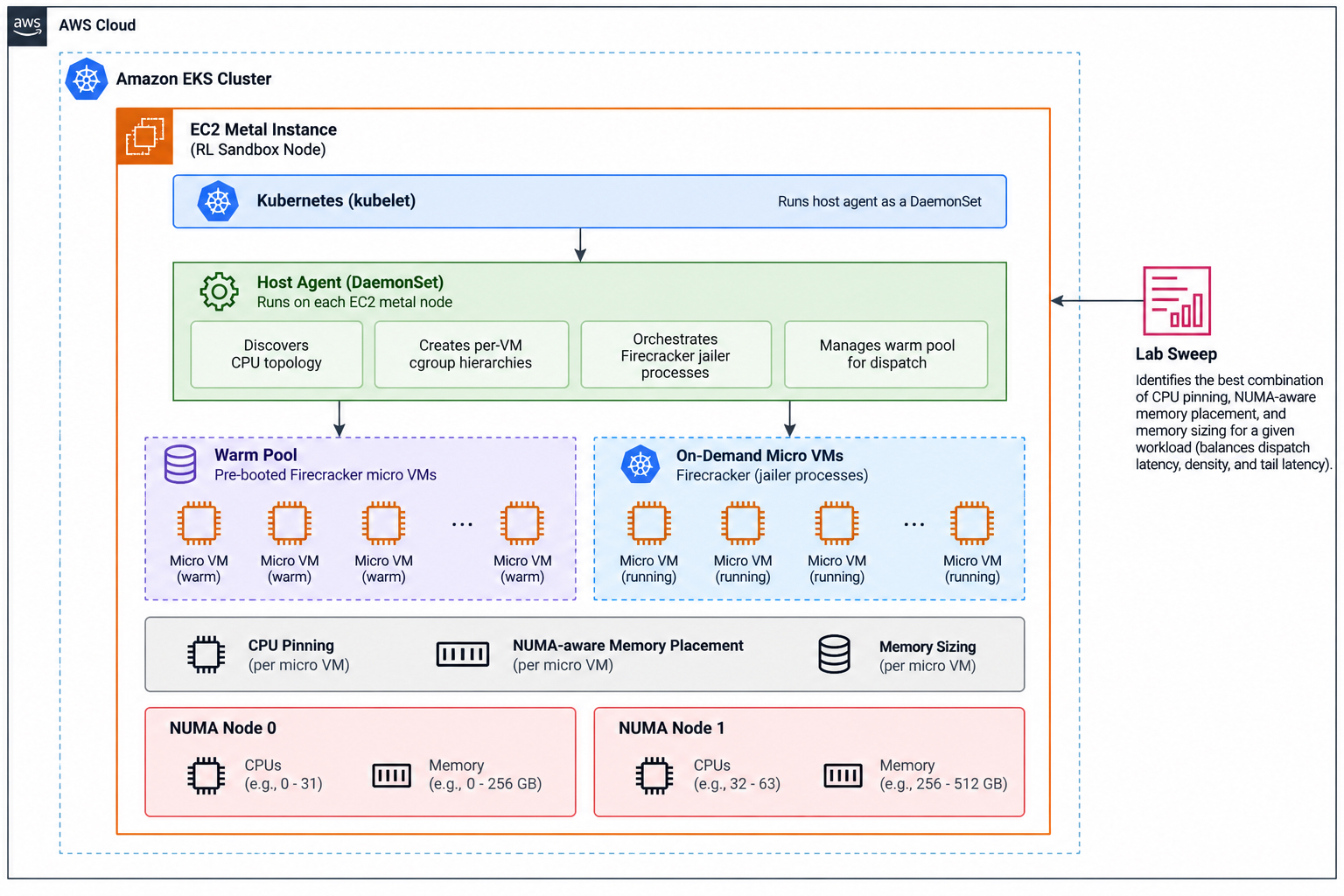
The host agent runs as a DaemonSet on each Amazon EC2 metal node in the Kubernetes cluster. At startup, it discovers the CPU topology, creates per-microVM cgroup hierarchies, and orchestrates Firecracker jailer processes throughout the microVM lifecycle.
To reduce dispatch latency, the system maintains a warm pool of pre-booted microVMs. The host agent applies CPU pinning, NUMA-aware memory placement, and memory sizing on a per-microVM basis. labsweep identifies the combination of these settings that best balances dispatch latency, density, and tail latency for a given workload.
Prerequisites
- Amazon EC2 metal instance (for example, we tested m8i.metal-48xl, m8a.metal-48xl, and m8g.metal-48xl).
- Linux kernel 6.2+ (required for
cgrouppartition isolated mode). - Firecracker 1.7+ and the Firecracker jailer.
- Go 1.22+ (to build
labsweep). - AWS CDK v2 with Python 3.11+ (to deploy the accompanying stack).
- Guest rootfs image (a builder script is included in the accompanying repository).
Scope note: this post focuses on CPU and memory placement for Firecracker microVMs. Other system variables including storage architecture (Amazon Elastic Block Store (Amazon EBS), local SSD) and network latency to the LLM endpoint were held constant to isolate the effects of CPU and memory placement.
Density tunables on EC2 metal
Your density ceiling depends on tunables whose availability varies by instance type. Not every knob exists on every instance type, and where a knob does exist its underlying mechanism can differ. The following table shows which tunables are available across the three metal instance types this post considers: m8i, m8a, and m8g. You can derive availability and mechanism from each instance type’s published CPU topology. The measured latency and throughput results later in the post currently cover m8i and m8a, with m8g results to follow.
| Tunable | m8i.metal-48xl | m8a.metal-48xl | m8g.metal-48xl | What it does |
Core pinning (cpuset.cpus) |
✓ | ✓ | ✓ | Dedicates a physical core to each microVM. Eliminates scheduler-induced tail latency |
NUMA node confinement (cpuset.mems) |
✓ | ✓ | ✓ (2 NUMA nodes on the 48xl) | Keeps memory allocations local. The remote-node latency penalty varies by instance type. Check the NUMA distance matrix for your instance before pinning |
| SMT state (smt/control) | ✓ (on/off) | N/A (no SMT) | N/A (no SMT) | Doubles vCPUs when on. Workload-dependent: helps I/O-bound sandboxes, hurts compute-bound loops |
| L3 cache domain pinning | ✓ (place workloads within NUMA-aligned cache domains) | ✓ (24 domains, 8 cores each) | ✓ (single shared L3 per socket. Pin on NUMA/socket boundary) | Reduces cache contention for working sets above 4 MiB per microVM |
cgroup partition (isolated) |
✓ | ✓ | ✓ | Removes kernel workqueue interference from pinned cores. Requires kernel 6.2+ |
| Guest memory size | ✓ | ✓ | ✓ | Primary cost driver. Determines how much of your memory-to-core budget each guest consumes; M-series gives 4 GiB per vCPU |
Key observation: different instance types expose different optimization opportunities. Among the instances evaluated, simultaneous multithreading (SMT) is available on m8i but not on m8a or m8g. Cache-local placement also differs by instance type: some present many discrete L3 domains, some a shared L3 that is effectively partitioned along NUMA boundaries, and some a single mesh-shared L3 per socket where the meaningful locality boundary is the NUMA/socket rather than a cache-domain count. Each instance type’s L3 layout is described in its own row of the table above and in its published CPU topology. As a result, the set of tunables and their impact on density vary by instance type. This is why measuring your own configuration matters more than following generic engineering best practice lists.
To make this concrete, here is what configuring one tunable looks like in practice: a cpuset pin that dedicates a single physical core to one microVM.
From tunables to measurement: labsweep
These tunables interact in ways that depend on your workload and instance type. You cannot predict their combined effect from the specification sheet alone. You must measure the resulting system behavior.
labsweep is the test harness we built to do exactly that. It is a Go tool that:
- Discovers your host topology through sysfs (cores, NUMA nodes, L3 domains).
- Plans a matrix of configurations and densities.
- Launches jailed Firecracker microVMs at each density with bounded concurrency.
- Runs the workload in every guest concurrently and records per-microVM latency.
- Outputs raw samples, percentile aggregates, and variance data with full host provenance.
Methodology note: each experiment is performed at fixed microVM density. Dynamic churn is outside the scope of this evaluation.
The following command launches a typical labsweep run on an m8a.metal-48xl:
Each run produces percentile latencies for every configuration, variance across repeated trials, and raw samples for recomputing any statistics. Results include full provenance (instance type, CPU model, kernel version, and Firecracker versions) making runs reproducible and comparable over time. If a microVM fails to respond, the harness reports failed samples instead of silently omitting them. This prevents failures from biasing the reported results.
The accompanying repository includes everything needed to reproduce these experiments: the labsweep harness, guest agent, rootfs builder, and the CDK application that deploys the complete stack on an Amazon EC2 metal instance (github.com/aws-samples/sample-firecracker-microvm-density-lab).
Results on representative workloads
Using labsweep we benchmarked workloads representative of the execution patterns in production RL systems: short-lived verification tasks (run a test suite, check the result), build-heavy tasks (compile and link), full 14-turn replayed RL episodes, and a synthetic compute loop as a control. Across all evaluated instance types, we collected more than 100,000 samples across 500+ configurations.
The 1.0x ratio rule
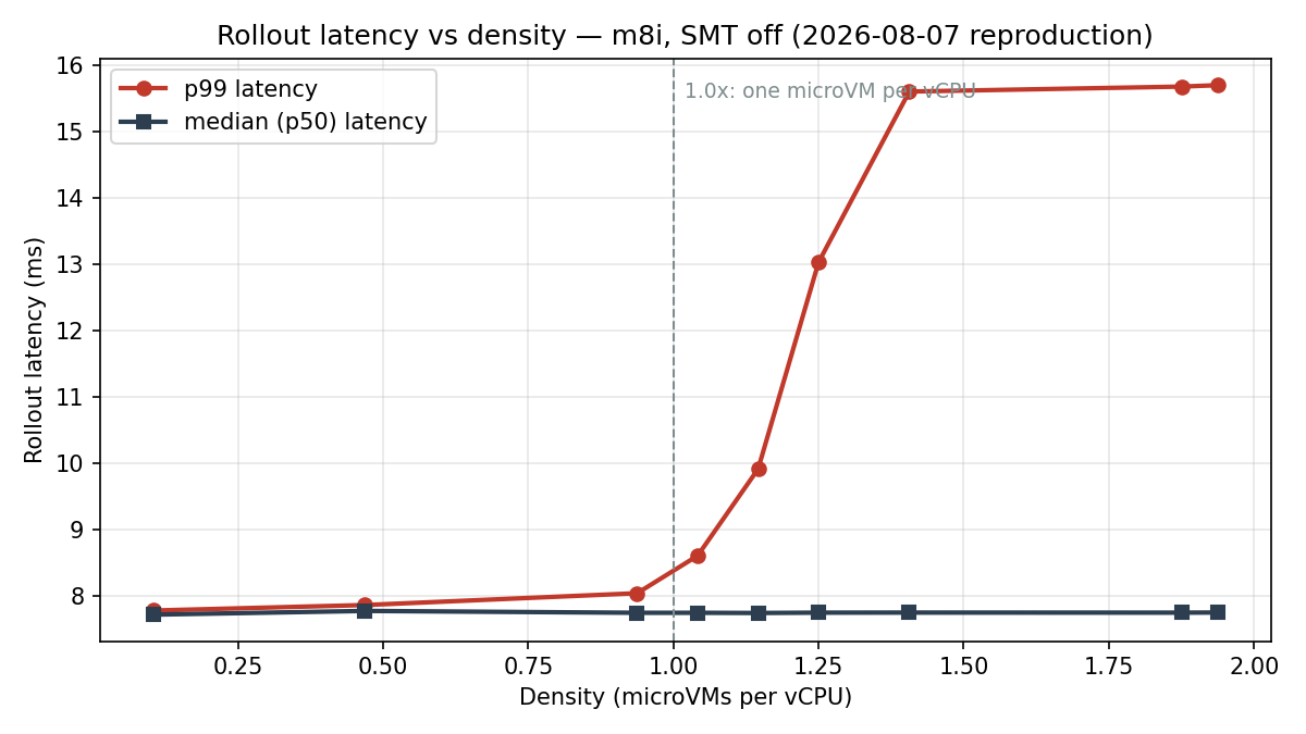
Tail latency remains flat as density increases until the workload reaches one microVM per vCPU. Beyond that threshold, p99 latency rises sharply over the next 15% increase in density before reaching a new plateau while median latency remains essentially unchanged. Expressing density as microVMs per vCPU rather than as an absolute microVM count makes this threshold portable across instance types. The latency cliff occurs at the same 1.0x density threshold regardless of instance size. Only the maximum number of microVMs scales with available vCPUs. The complete per-density measurements supporting this figure are provided in the appendix.
Core pinning reduces the tail latency for most real workloads
On the synthetic compute loop, core pinning made no measurable difference at equal density. On real sandbox workloads however, core pinning measurably tightened the tail: it reduced the p99/p50 ratio toward roughly 1.1x. The p99/p50 ratio measures tail spread by dividing the 99th-percentile latency by the median. Lower values indicate a tighter, more predictable latency distribution. The advantage grows with density, so pinning matters most where you are pushing the host hardest.
Why does this matter when choosing the right density? If you run Group Relative Policy Optimization (GRPO), every gradient step waits for the slowest rollout in the group. At a group size G=64, a p99 event affects ~47% of gradient steps. The effect becomes more pronounced as deployment density increases.
| Density / cores | G=8 | G=16 | G=64 |
| 0.94x | 1.01x | 1.01x | 1.04x |
| 1.04x | 1.01x | 1.03x | 1.13x |
| 1.15x | 1.01x | 1.04x | 1.32x |
Past the 1.0x ceiling the amplification climbs steadily, and by the time you are well above it a p99 event can dominate the group’s completion time. Median-focused dashboards do not surface this because the median stays flat. Core pinning keeps the p99/p50 ratio low across density, holding tail latency amplification far closer to flat than an unpinned configuration even at a group size of 64. Oversubscription can appear to provide spare capacity until tail latency amplification dominates training time. Set the density to the highest value where the amplification factor remains flat.
SMT depends on your workload
The optimal SMT setting depends on the workload:
- I/O-bound workloads: SMT-on provides higher throughput. At high density it delivers 1.49x throughput because the vCPU count stays above the 1.0x ratio.
- Compute-bound workloads: SMT-off produces more predictable tail latency, with a markedly tighter p99 spread than SMT-on.
Most RL sandbox workloads are I/O-bound, spending much of their time waiting on file operations, process creation, or git operations. For these workloads, keep SMT enabled. With SMT enabled, you can place more microVMs before reaching the 1.0x ratio, for higher density without crossing the latency cliff.
Configuration matters as much as hardware
Hardware selection is only one factor affecting performance. Configuration choices produce measurable differences. To isolate the effect of configuration, we compare identical workloads on the same m8i instance with SMT enabled and disabled. The results show that changing a single configuration parameter measurably affects peak throughput per host.
The table below shows how enabling and disabling SMT affects peak throughput across a representative set of RL workloads, expressed as the SMT-on to SMT-off throughput ratio. The workloads were selected to represent the major execution patterns encountered in RL systems. Collectively, they cover short-lived verification tasks, interactive sessions, and full RL episodes.
| Workload | Throughput gain from SMT |
| Verification task | 1.14x |
| Build task | 1.13x |
| Replayed RL episode | 1.17x |
The optimal SMT configuration depends on the density at which the workload is intended to run. With SMT enabled, the host exposes more vCPUs, which supports higher microVM densities before reaching the 1.0x microVM per vCPU threshold. This increases throughput at higher densities by delaying the onset of the tail latency cliff. At densities at or below one microVM per vCPU, SMT disabled delivers slightly better per-task performance and tighter tail latency. These results demonstrate that no single SMT configuration is universally optimal. The best choice depends on the target operating density. You should therefore determine the optimal configuration through measurement rather than assuming it in advance.
When memory becomes the limiting resource
We ran all experiments on M-series metal instances, which provide 4 GiB of memory per vCPU. At this memory-to-vCPU ratio, every workload we tested remained vCPU-bound. We exhausted vCPUs before memory. If your workloads require a higher memory-to-vCPU ratio, the bottleneck shifts from vCPUs to memory. In that case, a memory-optimized instance family may be the better choice. It provides more memory per vCPU but fewer vCPUs per host. As a result, the maximum sandbox density is lower. Consider this trade-off when selecting an instance family.
Reproduce these results on your own workloads
You do not need to take these numbers on faith. With labsweep, you can reproduce them on your own workloads. Clone the accompanying repository and deploy the CDK stack on the instance type you plan to run in production. Build a rootfs from your real workload. Sweep across densities below and above your expected level so you can see where expected performance drops off (the -densities flag in the preceding example is a reasonable start). Repeat each configuration a few times using the -repeats flag so you can see the variance, then read the p99/p50 ratio and the amplification table for your group size. Tune your system based on the curve you measure for your own workloads. That is more reliable than tuning to synthetic benchmarks.
Clean up
If you deployed the accompanying CDK stack for labsweep, tear down these resources when you are done:
- Delete the CDK stack (
cdk destroy). - Terminate any running Amazon EC2 metal instances.
- Remove the guest rootfs images from Amazon Simple Storage Service (Amazon S3) (if uploaded).
- Delete the Amazon CloudWatch log groups created by the harness.
Conclusion
Sandbox density on Amazon EC2 metal is determined by a small set of tunables whose optimal values depend on both the workload and the underlying instance type. Because those values vary across workloads, there is no single density setting or configuration that is optimal for every deployment. Instance type specifications give you a starting point but only measurement can identify the right operating point for your workload. labsweep is designed to make that measurement straightforward so you can optimize against your own production workloads.
Blog resources
Appendix
Full per-density measurements behind the tail-latency chart in “The 1.0x ratio rule.” Conditions: m8i, SMT off, 96 physical cores, config A (unpinned). Amplification columns give the GRPO group-completion factor (group max over rollout p50) at group sizes G=8, G=16, and G=64.
| Density | Density / cores | Rollout p50 | Rollout p99 | G=8 amp | G=16 amp | G=64 amp |
| 45 | 0.47x | 7,768 us | 7,857 us | 1.01 | 1.01 | 1.01 |
| 90 | 0.94x | 7,740 us | 8,035 us | 1.01 | 1.01 | 1.04 |
| 100 | 1.04x | 7,740 us | 8,601 us | 1.01 | 1.03 | 1.13 |
| 110 | 1.15x | 7,737 us | 9,909 us | 1.01 | 1.04 | 1.32 |
| 135 | 1.44x | 7,743 us | 15,601 us | 1.03 | 1.20 | 2.01 |
| 186 | 1.94x | 7,744 us | 15,697 us | 1.22 | 1.56 | 2.03 |