Post Syndicated from Suyash Nadkarni original https://aws.amazon.com/blogs/compute/tuning-guide-for-amd-amazon-ec2-instances/
As organizations migrate more mission-critical workloads to the cloud, optimizing for price-performance becomes a key consideration. Amazon Elastic Compute Cloud (Amazon EC2) instances powered by AMD EPYC processors deliver high core density, large memory bandwidth, and hardware-enabled security features, making them a strong option for a wide range of compute, memory, and I/O-intensive workloads. In this post, we explain how to choose the right AMD-based Amazon EC2 instance types and describe tuning techniques that can help users improve workload efficiency. Whether you’re running simulations, large-scale analytics, or inference workloads, this post provides practical guidance for optimizing AMD-powered Amazon EC2 instance.
Amazon EC2 offers AMD-based instances built on multiple generations of AMD EPYC processors. This post focuses on optimization strategies for the 3rd and 4th generation families, which provide enhanced capabilities for compute and memory-intensive workloads.
- 3rd generation (M6a, R6a, C6a, Hpc6a): Balances compute, memory, and storage—well-suited for analytics, web servers, and high-performance computing.
- 4th generation (M7a, R7a, C7a, Hpc7a): Deliver up to 50% better performance over earlier AMD generations These instances introduce AVX-512 support, DDR5 memory, and Simultaneous Multithreading (SMT) turned off, SMT is a technology that allows a single physical core to run multiple threads concurrently; with SMT disabled, each virtual CPU (vCPU) maps directly to a physical core, which can improve workload isolation and consistency.
Choosing the right AMD EPYC powered Amazon EC2 instance type
Selecting the right AMD EPYC powered Amazon EC2 instance type starts with understanding how your application uses compute, memory, storage, and networking resources. Each instance family is optimized for specific workload characteristics.
Compute-intensive workloads
These workloads involve large-scale calculations, simulations, or encoding tasks, and they often need high CPU throughput and advanced instruction set support.
Recommended instances: C7a, Hpc7a, C6a, Hpc6a
Use cases: Scientific computing, financial modelling, media transcoding, encryption, machine learning (ML) inference
Big data and analytics
Applications that process and analyze large datasets benefit from high memory bandwidth and a balanced compute-to-memory ratio.
Recommended instances: R7a, M7a, R6a, M6a
Use cases: Stream processing, real-time analytics, business intelligence tools, distributed caching
Database workloads
Database workloads typically need consistent memory performance and high I/O throughput for read/write operations.
Recommended instances: R7a, M7a, R6a, M6a
Use cases: Relational databases (MySQL, PostgreSQL), NoSQL databases (MongoDB, Cassandra), in-memory databases (Redis)
Web and application servers
These applications handle variable request loads and benefit from balanced compute, memory, and network performance.
Recommended instances: C7a, M7a, C6a, M6a
Use cases: Web servers, content management systems, e-commerce platforms, API endpoints
AI/ML on CPU
ML tasks that do not need GPUs—such as inference or preprocessing—can run efficiently on CPU-based instances.
Recommended instances: M7a, R7a, C7a
Use cases: Model inference, natural language processing, computer vision, recommendation engines
High Performance Computing (HPC)
These workloads need high core counts, memory bandwidth, and low-latency networking for tightly coupled computations.
Recommended instances: Hpc7a, Hpc6a, R7a, M7a
Use cases: Computational fluid dynamics, genomics, seismic analysis, engineering simulations
Aligning your instance type with the needs of your workload helps provide predictable performance and cost efficiency. Services such as Amazon EC2 Auto Scaling and AWS Compute Optimizer can assist with ongoing instance selection and scaling decisions.
Optimizing AMD EPYC powered Amazon EC2 instances
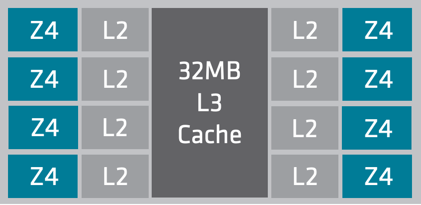
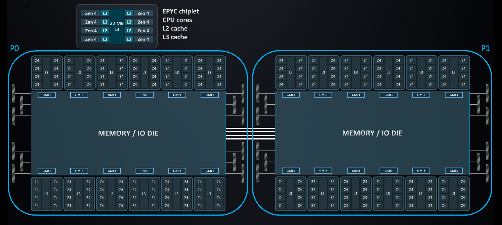
Amazon EC2 instances powered by 4th generation AMD EPYC processors use a modular chiplet architecture, as shown in the following figure. Each processor includes multiple Core Complex Dies (CCDs), and each CCD contains one or more core complexes (CCXs). A CCX groups up to eight physical cores, with each core having 1 MB of dedicated L2 cache and all eight cores sharing a 32 MB L3 cache. These CCDs are connected to a central I/O die, which manages memory and interconnects across the chip.

Figure 1: Layout of the ‘Zen 4’ CPU die with 8 cores per die
The modular architecture of 4th generation AMD EPYC processors enables Amazon EC2 instances such as m7a.24xlarge and m7a.48xlarge to support high core counts-up to 96 physical cores per socket. For example:
- m7a.24xlarge provides 96 physical cores from a single socket.
- m7a.48xlarge spans two sockets, offering 192 physical cores.
Understanding how Amazon EC2 instance sizes map to physical processor layouts can help you optimize for performance and cache locality. Workloads that involve shared memory access or thread synchronization, such as high-performance computing or in-memory databases, can benefit from selecting instance sizes that minimize cross-socket communication and make efficient use of shared L3 cache, as shown in the following figure.

Figure 2: Layout of the ‘EPYC Chiplet’ CPU
Amazon EC2 instances powered by 4th generation AMD EPYC processors operate with SMT turned off. In this configuration, each vCPU maps directly to a physical core, eliminating resource sharing such as execution units and cache between sibling threads. This design can reduce intra-core interference and help provide more consistent performance under certain workloads. Users can isolate threads at the core level and observe lower variability and more stable throughput for workloads, such as high-performance computing, ML inference, and transactional databases.
CPU optimizations
Tools such as htop can help identify CPU usage patterns, system load averages, and per-process resource consumption. CPU usage should be evaluated in the context of your workload and performance requirements. If usage consistently reaches 100%, then it may indicate that the workload is CPU-bound and not optimally balanced. Before modifying the instance size, enabling Auto Scaling, or switching instance families, evaluations must be conducted for the tuning opportunities that could improve performance without changing infrastructure. Load averages that regularly exceed the number of vCPUs can also signal compute saturation and may warrant further optimization.
L3 cache usage
The L3 cache is a shared, high-speed memory layer used by a group of CPU cores. On AMD-based Amazon EC2, cores are organized into L3 cache slices, each shared by a subset of cores on the same socket. Threads scheduled within the same slice can access shared data more efficiently, reducing memory latency. On 4th generation AMD instances such as m7a.2xlarge or r7a.2xlarge, all vCPUs typically map to cores within a single L3 slice, which ensures consistent cache locality. For larger sizes (for example m7a.8xlarge and above), thread pinning—assigning threads to specific physical cores—can help maintain this locality. Thread pinning can reduce performance variability in workloads with shared-memory access patterns.
You can pin threads using the taskset command:
taskset -c 0-3 ./your_application
This example pins your application to CPU cores 0 through 3. To determine which cores share the same L3 cache region, use tools such as lscpu or lstopo to inspect the system’s CPU topology. Grouping related threads on cores that share an L3 cache can improve performance consistency for workloads with frequent shared-memory access.
Docker container optimization
In containerized environments running on AMD-based Amazon EC2 instances, tuning CPU-related settings can improve workload consistency and efficiency—particularly for compute-intensive or latency-sensitive applications. Although default configurations work for many general-purpose scenarios, certain workloads may benefit from more explicit control over how CPU resources are allocated. By default, container runtimes such as Docker allow the operating system to schedule containers across any available CPU cores. This flexible scheduling can lead to variability in performance when containers move across cores that don’t share cache. To reduce this variability and improve cache efficiency, containers can be pinned to specific cores using the --cpuset-cpus flag.
docker run --cpuset-cpus="1,3" my-container
This setting restricts the container to use only the specified cores. In this example, cores 1 and 3 are used for demonstration. The actual core selection should be based on CPU topology to make sure of cache-efficient scheduling. Pinning containers to cores that share L3 cache can reduce scheduling overhead and improve consistency for workloads with shared-memory access patterns.
CPU frequency governor settings
Some operating systems adjust CPU frequency dynamically to save power. This is typically controlled by a setting called the CPU frequency governor. Although this behavior is efficient for general-purpose workloads, it may introduce latency or performance variability in compute-sensitive environments. For workloads that need consistently high CPU performance—such as high-throughput data processing, simulations, or real-time applications—we recommend setting the CPU governor to performance mode. This makes sure that the CPU runs at its maximum frequency under load, avoiding time spent ramping up from lower power states.
You can apply this setting on bare metal instances or Amazon EC2 Dedicated Hosts using the following command:
sudo cpupower frequency-set -g performance
Before applying, consider benchmarking workload performance with other CPU frequency governors (such as ondemand or schedutil) to make sure that the performance setting provides measurable benefits without unnecessary energy trade-offs.
Use architecture-specific compiler flags
When compiling performance-sensitive C or C++ applications, architecture-specific flags such as -march=znverX can unlock AMD EPYC–specific optimizations, including improved vectorization and floating-point performance. Although this is beneficial for compute-heavy workloads, it may reduce portability across architectures. To balance performance and flexibility, consider implementing runtime feature detection and dispatching an approach used by many optimized libraries to adapt behavior based on the underlying CPU.
Before using these flags, verify that your compiler version supports them and make sure that the target EC2 instance architecture matches the specified flag. For example, a binary compiled with -march=znver4 may fail with an illegal instruction error (SIGILL) if run on earlier-generation instances such as M5a.The following table outlines the appropriate flags and minimum supported compiler versions for each AMD EPYC generation:
| AMD EPYC Generation |
-march Flag |
Minimum GCC Version |
Minimum LLVM/Clang Version |
| 4th generation (for example M7a) |
znver4 |
GCC 12 |
Clang 15 |
| 3rd generation (for example M6a) |
znver3 |
GCC 11 |
Clang 13 |
| 2nd generation (for example M5a) |
znver2 |
GCC 9 |
Clang 11 |
The following flags are supported for GCC 11+ or LLVM Clang 13+:
# 4th Gen EPYC (M7a, R7a, C7a, Hpc7a)
-march=znver4

# 3rd Gen EPYC (M6a, R6a, C6a)
-march=znver3

# 2nd Gen EPYC (M5a, R5a, C5a)
-march=znver2
When to enable AVX-512 and VNNI instructions
4th generation AMD EPYC powered Amazon EC2 instances support advanced single instruction, multiple data (SIMD) instruction sets such as AVX2, AVX-512, and VNNI. These can improve throughput for vector-heavy workloads such as ML inference, image processing, or scientific simulations. However, these flags are generation-specific—attempting to run binaries compiled with AVX-512 on unsupported instances (for example 2nd generation M5a) may result in runtime errors such as illegal instruction (SIGILL).
When compiling C or C++ code:
gcc -mavx2 -mavx512f -O2 your_program.c -o your_program
To better understand which optimizations are applied, use the following:
-ftree-vectorizer-verbose=2 -fopt-info-vec-missed
This helps identify loops that benefit from vectorization and those that don’t. Only enable these optimizations if your workload benefits and you’ve validated compatibility with the instance generation in use. Avoid applying AVX flags indiscriminately, because it may reduce portability and increase binary complexity.
AMD Optimizing CPU Libraries
The AMD Optimizing CPU Libraries (AOCL) provide performance-tuned math libraries specifically designed for AMD EPYC processors. These libraries include optimized implementations of commonly used functions in scientific computing, engineering, and ML workloads. You can link your applications against AOCL to use processor-specific optimizations without rewriting your code. AOCL includes libraries for vector and scalar math, random number generation, FFT, BLAS, and LAPACK, among others.
Setting up AOCL
- Set the AOCL_ROOT environment variable to point to the installation directory:
export AOCL_ROOT=/path/to/aocl
- Compile your application with the appropriate include and library paths:
gcc -I$AOCL_ROOT/include -L$AOCL_ROOT/lib -lamdlibm -lm your_program.c -o your_program
- Vector and scalar math optimization: you can enable more vectorized or scalar math tuning flags for specific workloads:
# Vector math optimization
gcc -lamdlibm -fveclib=AMDLIBM -lm your_program.c -o your_program

# Faster scalar math
gcc -lamdlibm -fsclrlib=AMDLIBM -lamdlibmfast -lm your_program.c -o your_program
- AOCL runtime profiling: AOCL supports runtime profiling, which helps developers identify which mathematical operations dominate execution time. To enable profiling, run the following:
export AOCL_PROFILE=1
./your_program
After running this, a report file named aocl_profile_report.txt is generated. It provides a function-level breakdown of call counts, execution time, and thread usage. Developers can use this to focus optimization efforts on high-impact operations.
Conclusion
This post explored how to select AMD-based Amazon EC2 instance types that align with specific workload characteristics, and how to apply tuning techniques focused on CPU usage, thread placement, cache efficiency, and math library optimization. These approaches are especially relevant for compute-bound or latency-sensitive workloads where consistent performance is critical.
Ready to get started? Sign in to the AWS Management Console and launch AMD EPYC powered Amazon EC2 instances to begin optimizing your workloads today.