Tag Archives: Amazon Redshift

Amazon S3 Storage Lens adds performance metrics, support for billions of prefixes, and export to S3 Tables

2025-12-02 Veliswa Boya

Post Syndicated from Veliswa Boya original https://aws.amazon.com/blogs/aws/amazon-s3-storage-lens-adds-performance-metrics-support-for-billions-of-prefixes-and-export-to-s3-tables/

Today, we’re announcing three new capabilities for Amazon S3 Storage Lens that give you deeper insights into your storage performance and usage patterns. With the addition of performance metrics, support for analyzing billions of prefixes, and direct export to Amazon S3 Tables, you have the tools you need to optimize application performance, reduce costs, and make data-driven decisions about your Amazon S3 storage strategy.

New performance metric categories
S3 Storage Lens now includes eight new performance metric categories that help identify and resolve performance constraints across your organization. These are available at organization, account, bucket, and prefix levels. For example, the service helps you identify small objects in a bucket or prefix that can slow down application performance. This can be mitigated by batching small objects or using the Amazon S3 Express One Zone storage class for higher performance small object workloads.

To access the new performance metrics, you need to enable performance metrics in the S3 Storage Lens advanced tier when creating a new Storage Lens dashboard or editing an existing configuration.

Metric category	Details	Use case	Mitigation
Read request size	Distribution of read request sizes (GET) by day	Identify dataset with small read request patterns that slow down performance	Small request: Batch small objects or use Amazon S3 Express One Zone for high-performance small object workloads
Write request size	Distribution of write request sizes (PUT, POST, COPY, and UploadPart) by day	Identify dataset with small write request patterns that slow down performance	Large request: Parallelize requests, use MPU or use AWS CRT
Storage size	Distribution of object sizes	Identify dataset with small small objects that slow down performance	Small object sizes: Consider bundling small objects
Concurrent PUT 503 errors	Number of 503s due to concurrent PUT operation on same object	Identify prefixes with concurrent PUT throttling that slow down performance	For single writer, modify retry behavior or use Amazon S3 Express One Zone. For multiple writers, use consensus mechanism or use Amazon S3 Express One Zone
Cross-Region data transfer	Bytes transferred and requests sent across Region, in Region	Identify potential performance and cost degradation due to cross-Region data access	Co-locate compute with data in the same AWS Region
Unique objects accessed	Number or percentage of unique objects accessed per day	Identify datasets where small subset of objects are being frequently accessed. These can be moved to higher performance storage tier for better performance	Consider moving active data to Amazon S3 Express One Zone or other caching solutions
FirstByteLatency (existing Amazon CloudWatch metric)	Daily average of first byte latency metric	The daily average per-request time from the complete request being received to when the response starts to be returned
TotalRequestLatency (existing Amazon CloudWatch metric)	Daily average of Total Request Latency	The daily average elapsed per request time from the first byte received to the last byte sent

How it works
On the Amazon S3 console I choose Create Storage Lens dashboard to create a new dashboard. You can also edit an existing dashboard configuration. I then configure general settings such as providing a Dashboard name, Status, and the optional Tags. Then, I choose Next.

Next, I define the scope of the dashboard by selecting Include all Regions and Include all buckets and specifying the Regions and buckets to be included.

I opt in to the Advanced tier in the Storage Lens dashboard configuration, select Performance metrics, then choose Next.

Next, I select Prefix aggregation as an additional metrics aggregation, then leave the rest of the information as default before I choose Next.

I select the Default metrics report, then General purpose bucket as the bucket type, and then select the Amazon S3 bucket in my AWS account as the Destination bucket. I leave the rest of the information as default, then select Next.

I review all the information before I choose Submit to finalize the process.

After it’s enabled, I’ll receive daily performance metrics directly in the Storage Lens console dashboard. You can also choose to export report in CSV or Parquet format to any bucket in your account or publish to Amazon CloudWatch. The performance metrics are aggregated and published daily and will be available at multiple levels: organization, account, bucket, and prefix. In this dropdown menu, I choose the % concurrent PUT 503 error for the Metric, Last 30 days for the Date range, and 10 for the Top N buckets.

The Concurrent PUT 503 error count metric tracks the number of 503 errors generated by simultaneous PUT operations to the same object. Throttling errors can degrade application performance. For a single writer, modify retry behavior or use higher performance storage tier such as Amazon S3 Express One Zone to mitigate concurrent PUT 503 errors. For multiple writers scenario, use a consensus mechanism to avoid concurrent PUT 503 errors or use higher performance storage tier such as Amazon S3 Express One Zone.

Complete analytics for all prefixes in your S3 buckets
S3 Storage Lens now supports analytics for all prefixes in your S3 buckets through a new Expanded prefixes metrics report. This capability removes previous limitations that restricted analysis to prefixes meeting a 1% size threshold and a maximum depth of 10 levels. You can now track up to billions of prefixes per bucket for analysis at the most granular prefix level, regardless of size or depth.

The Expanded prefixes metrics report includes all existing S3 Storage Lens metric categories: storage usage, activity metrics (requests and bytes transferred), data protection metrics, and detailed status code metrics.

How to get started
I follow the same steps outlined in the How it works section to create or update the Storage Lens dashboard. In Step 4 on the console, where you select export options, you can select the new Expanded prefixes metrics report. Thereafter, I can export the expanded prefixes metrics report in CSV or Parquet format to any general purpose bucket in my account for efficient querying of my Storage Lens data.

Good to know
This enhancement addresses scenarios where organizations need granular visibility across their entire prefix structure. For example, you can identify prefixes with incomplete multipart uploads to reduce costs, track compliance across your entire prefix structure for encryption and replication requirements, and detect performance issues at the most granular level.

Export S3 Storage Lens metrics to S3 Tables
S3 Storage Lens metrics can now be automatically exported to S3 Tables, a fully managed feature on AWS with built-in Apache Iceberg support. This integration provides daily automatic delivery of metrics to AWS managed S3 Tables for immediate querying without requiring additional processing infrastructure.

How to get started
I start by following the process outlined in Step 5 on the console, where I choose the export destination. This time, I choose Expanded prefixes metrics report. In addition to General purpose bucket, I choose Table bucket.

The new Storage Lens metrics are exported to new tables in an AWS managed bucket aws-s3.

I select the expanded_prefixes_activity_metrics table to view API usage metrics for expanded prefix reports.

I can preview the table on the Amazon S3 console or use Amazon Athena to query the table.

Good to know
S3 Tables integration with S3 Storage Lens simplifies metric analysis using familiar SQL tools and AWS analytics services such as Amazon Athena, Amazon QuickSight, Amazon EMR, and Amazon Redshift, without requiring a data pipeline. The metrics are automatically organized for optimal querying, with custom retention and encryption options to suit your needs.

This integration enables cross-account and cross-Region analysis, custom dashboard creation, and data correlation with other AWS services. For example, you can combine Storage Lens metrics with S3 Metadata to analyze prefix-level activity patterns and identify objects in prefixes with cold data that are eligible for transition to lower-cost storage tiers.

For your agentic AI workflows, you can use natural language to query S3 Storage Lens metrics in S3 Tables with the S3 Tables MCP Server. Agents can ask questions such as ‘which buckets grew the most last month?’ or ‘show me storage costs by storage class’ and get instant insights from your observability data.

Now available
All three enhancements are available in all AWS Regions where S3 Storage Lens is currently offered (except the China Regions and AWS GovCloud (US)).

These features are included in the Amazon S3 Storage Lens Advanced tier at no additional charge beyond standard advanced tier pricing. For the S3 Tables export, you pay only for S3 Tables storage, maintenance, and queries. There is no additional charge for the export functionality itself.

To learn more about Amazon S3 Storage Lens performance metrics, support for billions of prefixes, and export to S3 Tables, refer to the Amazon S3 user guide. For pricing details, visit the Amazon S3 pricing page.

Veliswa Boya.

Achieve 2x faster data lake query performance with Apache Iceberg on Amazon Redshift

2025-11-27 Kalaiselvi Kamaraj

Post Syndicated from Kalaiselvi Kamaraj original https://aws.amazon.com/blogs/big-data/achieve-2x-faster-data-lake-query-performance-with-apache-iceberg-on-amazon-redshift/

With the growing adoption of open table formats like Apache Iceberg, Amazon Redshift continues to advance its capabilities for open format data lakes. In 2025, Amazon Redshift delivered several performance optimizations that improved query performance over twofold for Iceberg workloads on Amazon Redshift Serverless, delivering exceptional performance and cost-effectiveness for your data lake workloads.

In this post, we describe some of the optimizations that led to these performance gains. Data lakes have become a foundation of modern analytics, helping organizations store vast amounts of structured and semi-structured data in cost-effective data formats like Apache Parquet while maintaining flexibility through open table formats. This architecture creates unique performance optimization opportunities across the entire query processing pipeline.

Performance enhancements

Our latest enhancements span multiple areas of the Amazon Redshift SQL query processing engine, including vectorized scanners that accelerate execution, optimal query plans powered by just-in-time (JIT) runtime statistics, distributed Bloom filters, and new decorrelation rules.

The following chart summarizes the performance improvements achieved so far in 2025, as measured by industry standard 10 TB TPC-DS and TPC-H benchmarks run on Iceberg tables on an 88 RPU Redshift Serverless endpoint.

Find the best performance for your workloads

The performance results presented in this post are based on benchmarks derived from the industry-standard TPC-DS and TPC-H benchmarks, and have the following characteristics:

The schema and data of Iceberg tables are used unmodified from TPC-DS. Tables are partitioned to reflect real-world data organization patterns.
The queries are generated using the official TPC-DS and TPC-H kits with query parameters generated using the default random seed of the kits.
The TPC-DS test includes all 99 TPC-DS SELECT queries. It doesn’t include maintenance and throughput steps. The TPC-H test includes all 22 TPC-H SELECT queries.
Benchmarks are run out of the box: no manual tuning or stats collection is done for the workloads.

In the following sections, we discuss key performance improvements delivered in 2025.

Faster data lake scans

To improve data lake read performance, the Amazon Redshift team built a completely new scan layer designed from the ground-up for data lakes. This new scan layer includes a purpose-built I/O subsystem, incorporating smart prefetch capabilities to reduce data latency. Additionally, the new scan layer is optimized for processing Apache Parquet files, the most commonly used file format for Iceberg, through fast vectorized scans.

This new scan layer also includes sophisticated data pruning mechanisms that operate at both partition and file levels, dramatically reducing the volume of data that needs to be scanned. This pruning capability works in harmony with the smart prefetch system, creating a coordinated approach that maximizes efficiency throughout the entire data retrieval process.

JIT ANALYZE for Iceberg tables

Unlike traditional data warehouses, data lakes often lack comprehensive table- and column-level statistics about the underlying data, making it challenging for the planner and optimizer in the query engine to choose up-front which execution plan will be most optimal. Sub-optimal plans can lead to slower and less predictable performance.

JIT ANALYZE is a new Amazon Redshift feature that automatically collects and uses statistics for Iceberg tables during query execution—minimizing manual statistics collection while giving the planner and optimizer in the query engine the information it needs to generate optimal query plans. The system uses intelligent heuristics to identify queries that will benefit from statistics, performs fast file-level sampling using Iceberg metadata, and extrapolates population statistics using advanced techniques.

JIT ANALYZE delivers out-of-the-box performance nearly equal to queries that have pre-calculated statistics, while providing the foundation for many other performance optimizations. Some TPC-DS queries improved by 50 times faster with these statistics.

Query optimizations

For correlated subqueries such as those that contain EXISTS/IN clauses, Amazon Redshift uses decorrelation rules to rewrite the queries. In many cases, these decorrelation rules were not producing optimal plans, resulting in query execution performance regressions. To address this, we introduced a new internal join type, SEMI JOIN, and a new decorrelation rule based on this join type. This decorrelation rule helps in producing the most optimal plans, thereby improving execution performance. For instance, one of the TPC-DS queries that contains EXIST clause ran 7 times faster with this optimization.

We introduced distributed Bloom filter optimization for data lake workloads. Distributed Bloom filters create Bloom filters locally in every compute node and then distributes them to every other node. Distributing Bloom filters can significantly reduce the amount of data that needs to be sent over the network for the join by filtering out the tuples earlier. This provides good performance gains for large, complex data lake queries that process and join large amounts of data.

Conclusion

These performance improvements for Iceberg workloads represent a major leap forward in Redshift data lake capabilities. By focusing on out-of-the-box performance, we’ve made it straightforward to achieve exceptional query performance without complex tuning or optimization.

These improvements demonstrate the power of deep technical innovation combined with practical customer focus. JIT ANALYZE reduces the operational burden of statistics management while providing optimal query planning information. The new Redshift data lake query engine on Redshift Serverless was rewritten from the ground up for best-in-class scan performance, and lays the groundwork for more advanced performance optimizations. Semi-join optimizations tackle some of the most challenging query patterns in analytical workloads. You can run complex analytical workloads on your Iceberg data and get fast, predictable query performance.

Amazon Redshift is committed to being the best analytics engine for data lake workloads, and these performance optimizations represent our continued investment in that goal.

To learn more about Amazon Redshift and its performance capabilities, visit the Amazon Redshift product page. To get started with Redshift, you can try Amazon Redshift Serverless and start querying data in minutes without having to set up and manage data warehouse infrastructure. For more details on performance best practices, see the Amazon Redshift Database Developer Guide. To stay up-to-date with the latest developments in Amazon Redshift, subscribe to the What’s New in Amazon Redshift RSS feed.

Special thanks to this post’s contributors: Martin Milenkoski, Gerard Louw, Konrad Werblinski, Mengchu Cai, Mehmet Bulut, Mohammed Alkateb, and Sanket Hase

Getting started with Apache Iceberg write support in Amazon Redshift

2025-11-26 Sanket Hase

Post Syndicated from Sanket Hase original https://aws.amazon.com/blogs/big-data/getting-started-with-apache-iceberg-write-support-in-amazon-redshift/

Many companies store structured data in warehouses for analytics while keeping diverse datasets in data lakes for flexible processing. Until now, maintaining consistency between these systems required complex ETL processes and introduced potential data synchronization challenges.

The new Amazon Redshift Apache Iceberg write support removes these complexities through direct writes to Apache Iceberg tables stored in Amazon S3 and S3 Tables. With this native integration you can write data directly from Redshift queries to your data lake without intermediate ETL steps, facilitate data consistency with ACID-compliant transactions that help optimize query performance with flexible partitioning strategies, and use the familiar Redshift SQL interface when writing to Apache Iceberg tables. For example, you can now run a complex transformation in Redshift and write the results directly to an Apache Iceberg table that other analytics engines like Amazon EMR or Amazon Athena can immediately query. By using this approach you can query the same datasets from both Redshift and other analytics tools without copying data.

In this post, we show how you can use Amazon Redshift to write data directly to Apache Iceberg tables stored in Amazon S3 and S3 Tables for seamless integration between your data warehouse and data lake while maintaining ACID compliance.

“Verisk processes billions of catastrophe risk modeling records using Amazon Redshift and Apache Iceberg, achieving 30% faster query aggregations and significant storage cost reductions”

— Karthick Shanmugam, Associate Vice President, Verisk

Solution overview

You can now create and write directly to Apache Iceberg tables stored in Amazon S3 and S3 Tables using familiar SQL commands in Amazon Redshift. We’ll guide you through configuring permissions for S3 table buckets using AWS Lake Formation. Finally, we’ll analyze customer and order datasets across both Redshift native and Apache Iceberg data formats to derive insights. The workflow is illustrated in the following diagram:

In this post we will walk you through following steps:

Create an external database named customer_db in AWS Glue Data Catalog using Amazon Redshift SQL.
Create an external table named customer in the Glue database and write customer data using Amazon Redshift SQL.
Create table bucket named orders on Amazon S3 Tables to write orders data.
Grant permissions using AWS Lake Formation to an IAM role for reading and writing to the orders table.
Write orders data to the orders Amazon S3 table bucket.

This solution uses the following AWS services:

Prerequisites

Create Amazon Redshift data warehouse (provisioned or Serverless).
Permissions to create database on AWS Glue Data Catalog from Redshift.
Create a new AWS Glue database called customer_db or use an existing database of your choice. If you use an existing database or a different name, replace customer_db with your actual database name in the subsequent commands.
S3 bucket and S3 Table bucket in the same AWS Region as your Redshift cluster.
Have access to an IAM role that is a Lake Formation data lake administrator. For instructions, refer to Create a data lake administrator.

Create IAM role RedshifticebergRole with following policy. Add managed permission for AmazonRedshiftQueryEditorV2.

{
    "Version": "2012-10-17",
    "Statement": [
                    {
                        "Sid": "VisualEditor0",
                        "Effect": "Allow",
                        "Action": "redshift:GetClusterCredentialsWithIAM",
                        "Resource": "arn:aws:redshift:<YOUR-REGION>:<AWS-ACCOUNT-NUMBER>:dbname::<YOUR-REDSHIFT-CLUSTER-NAME>/*"
                    }
                ]
}

Setting up your environment

To set up your environment, complete the following steps.

Creating Apache Iceberg tables in Amazon S3 standard buckets

Connect to Redshift using Query Editor V2.
Create user for the Federated role RedshifticebergRole.
```
Create user IAMR:RedshifticebergRole
```

Verify you have an Amazon Redshift External Schema configured. Run following script on Redshift:

CREATE EXTERNAL SCHEMA demo_iceberg
FROM DATA CATALOG DATABASE 'customer_db'
IAM_ROLE 'arn:aws:iam::<AWS-ACCOUNT-NUMBER>:role/RedshiftCustomizedIcebergRole';

Create external table customer in Apache Iceberg table format in the demo_iceberg external schema created above and then insert data.

Use this two-step approach when you need control over column definitions or plan to append data.

Replace your S3 bucket name in place of <<your-bucket>>.

-- Step 1: Define your table structure
CREATE TABLE demo_iceberg.customer
(
customer_id bigint,
customer_name varchar,
email varchar,
city varchar
)
USING ICEBERG
LOCATION 's3://<<your-bucket>>/iceberg-data/customers/';

-- Step 2: Insert data
              
(1, 'Customer1 Smith', '[email protected]', 'New York'),
(2, 'Customer2 Johnson', '[email protected]', 'Los Angeles'),
(3, 'Customer3 Brown', '[email protected]', 'Chicago'),
(4, 'Customer4 Davis', '[email protected]', 'Houston'),
(5, 'Customer5 Wilson', '[email protected]', 'Phoenix'),
(6, 'Customer6 Miller', '[email protected]', 'Philadelphia'),
(7, 'Customer7 Garcia', '[email protected]', 'San Antonio'),
(8, 'Customer8 Rodriguez', '[email protected]', 'San Diego'),
(9, 'Customer9 Martinez', '[email protected]', 'Dallas'),
(10, 'Customer10 Anderson', '[email protected]', 'San Jose'),
(11, 'Customer11 Taylor', '[email protected]', 'Austin'),
(12, 'Customer12 Thomas', '[email protected]', 'Jacksonville'),
(13, 'Customer13 Jackson', '[email protected]', 'Fort Worth'),
(14, 'Customer14 White', '[email protected]', 'Columbus'),
(15, 'Customer15 Harris', '[email protected]', 'Charlotte');

-- Step 3: Select data
SELECT * FROM demo_iceberg.customer;

Figure 2: Result from demo_iceberg.customer

Grant access to external schema for user IAMR:RedshifticebergRole:

Grant usage on schema demo_iceberg to "IAMR:RedshifticebergRole";

Create Apache Iceberg tables in Amazon S3 Table buckets

Amazon S3 table buckets are integrated with AWS Lake Formation, which serves as the central authority for managing data access permissions. When working with Apache Iceberg tables, Lake Formation provides a unified security framework that simplifies access control across your entire data lake. This centralized approach makes sure consistent and efficient permission management, alleviating the need to handle permissions in multiple places.

To create an S3 table bucket:

Go to Amazon S3, choose Table buckets in the left navigation pane.
On the Table buckets page, in the Integration with AWS analytics services section, choose Enable integration.
In the Table buckets list, choose the Create table bucket button and enter a name for your table bucket, for example, iceberg-write-blog, and choose Create table bucket. After creation, the bucket will appear in the S3 tables catalog, s3tablescatalog, in the Lake Formation console.
In the AWS Lake Formation console, choose Catalogs, in the Catalogs table select s3tablescatalog to open the detail page for that table.
On the s3tablescatalog details page, under Catalogs, choose the table bucket iceberg-write-blog.
On the iceberg-write-blog details page, under Databases, choose Create database.
Enter the database name iceberg_write_namespace, select the Catalog from the drop down menu, and choose Create database.
Grant a permission to create a table in the database to the Lake Formation IAM role. On the iceberg-write-blog details page select the radio button for iceberg_write_namespace, choose Actions, Grant.
On the Grant permissions page, under Principal type select Principals, under Principals select IAM users and roles, in the IAM users and roles drop down menu select RedshifticebergRole.
For LF-Tags or catalog resources, choose Named Data Catalog resources, for Catalogs select iceberg-write-blog and for Databases select iceberg_write_namespace.
For Database permissions select the checkbox for Create table, Drop, and Describe, then choose Grant.

Creating Apache Iceberg tables in Amazon Redshift using Amazon S3 table buckets

AWS Lake Formation catalogs are automatically mounted on Amazon Redshift data warehouses in same account. Amazon Redshift writes directly to S3 Tables using the auto mounted S3 table catalog. The SQL syntax for writing to Apache Iceberg tables stored in S3 table buckets is similar to the syntax for Apache Iceberg tables stored in S3 standard buckets. The key difference is the auto mounted S3 Table catalog, which supports three-part notation access. This feature alleviates the need to create an EXTERNAL SCHEMA when referencing data lake Apache Iceberg tables residing in S3 Table buckets.

To create the Apache Iceberg table:

Switch to the RedshifticebergRole. To access S3 tables through the Redshift Query Editor V2, you must use a Federated user account, the RedshifticebergRole has been granted the necessary Lake Formation permissions.
Log in to Redshift using the Query Editor V2 Federated user option.

In Query Editor V2, create the table named orders in Apache Iceberg table format:

CREATE TABLE "iceberg-write-blog@s3tablescatalog".iceberg_write_namespace.orders
(
 customer_id BIGINT,
 order_id BIGINT,
 Total_order_amt DECIMAL(10,2),
 Total_order_tax_amt REAL,
 tax_pct DOUBLE PRECISION,
 order_date DATE,
 order_created_at_tz TIMESTAMPTZ,
 is_active_ind BOOLEAN
)
USING ICEBERG 
PARTITIONED BY (DAY(order_date));

Insert data into the table using standard SQL:

INSERT INTO "iceberg-write-blog@s3tablescatalog".iceberg_write_namespace.orders
(order_date, order_id, customer_id, total_order_amt, total_order_tax_amt, tax_pct, order_created_at_tz, is_active_ind)
VALUES
('2024-01-15', 1001, 1, 125.50, 10.04, 0.08, '2024-01-15 10:30:00-06:00', true),
('2024-02-20', 1002, 2, 89.99, 6.75, 0.075, '2024-02-20 14:22:15-06:00', true),
('2024-03-10', 1003, 3, 234.75, 20.78, 0.0885, '2024-03-10 09:15:30-06:00', false),
('2024-04-05', 1004, 1, 67.25, 5.38, 0.08, '2024-04-05 16:45:00-05:00', true),
('2024-05-18', 1005, 4, 156.80, 12.54, 0.08, '2024-05-18 11:20:45-05:00', true),
('2024-06-22', 1006, 5, 45.99, 4.14, 0.09, '2024-06-22 13:10:20-05:00', true),
('2024-07-14', 1007, 2, 312.40, 24.99, 0.08, '2024-07-14 08:35:10-05:00', false),
('2024-08-30', 1008, 6, 78.50, 7.07, 0.09, '2024-08-30 15:25:35-05:00', true),
('2024-09-12', 1009, 3, 199.99, 18.00, 0.09, '2024-09-12 12:40:50-05:00', true),
('2024-10-08', 1010, 7, 523.75, 41.90, 0.08, '2024-10-08 17:15:25-05:00', true),
('2024-10-25', 1011, 4, 92.30, 8.31, 0.09, '2024-10-25 10:05:15-05:00', false),
('2024-11-02', 1012, 8, 167.45, 13.40, 0.08, '2024-11-02 14:50:40-06:00', true),
('2024-11-08', 1013, 1, 34.99, 2.80, 0.08, '2024-11-08 09:30:20-06:00', true),
('2024-11-09', 1014, 9, 445.60, 40.10, 0.09, '2024-11-09 16:20:55-06:00', true),
('2024-11-10', 1015, 5, 278.85, 22.31, 0.08, '2024-11-10 11:45:30-06:00', true);

Create a Redshift local_orders table and insert sample records:

CREATE TABLE dev.public.local_orders
(
customer_id BIGINT,
order_id BIGINT,
Total_order_amt DECIMAL(10,2),
Total_order_tax_amt REAL,
tax_pct DOUBLE PRECISION,
order_date DATE,
order_created_at_tz TIMESTAMPTZ,
is_active_ind BOOLEAN
);


INSERT INTO dev.public.local_orders
(customer_id, order_id, Total_order_amt, Total_order_tax_amt, tax_pct, order_date, order_created_at_tz, is_active_ind)
VALUES
(1001, 5001, 299.99, 24.00, 0.08, '2024-01-15', '2024-01-15 14:30:00-05:00', true),
(1002, 5002, 1250.50, 100.04, 0.08, '2024-01-16', '2024-01-16 09:15:22-05:00', true),
(1003, 5003, 75.25, 6.02, 0.08, '2024-01-16', '2024-01-16 16:45:33-05:00', true),
(1004, 5004, 499.99, 40.00, 0.08, '2024-01-17', '2024-01-17 11:20:45-05:00', true),
(1005, 5005, 149.50, 11.96, 0.08, '2024-01-17', '2024-01-17 13:55:12-05:00', false),
(1002, 5006, 899.99, 72.00, 0.08, '2024-01-18', '2024-01-18 10:05:30-05:00', true),
(1006, 5007, 45.75, 3.66, 0.08, '2024-01-18', '2024-01-18 15:40:18-05:00', true),
(1007, 5008, 1500.00, 120.00, 0.08, '2024-01-19', '2024-01-19 08:25:55-05:00', true),
(1008, 5009, 250.25, 20.02, 0.08, '2024-01-19', '2024-01-19 12:10:40-05:00', true),
(1009, 5010, 725.75, 58.06, 0.08, '2024-01-20', '2024-01-20 14:15:28-05:00', true);

Using the CREATE TABLE AS (CTAS) format, create a table from the existing table with no compression:

CREATE TABLE "iceberg-write-blog@s3tablescatalog".iceberg_write_namespace.orders_new 
using ICEBERG
TABLE PROPERTIES ('compression_type'='uncompressed')
AS
select * from dev.public.local_orders;

Select data with standard SQL using the three-part notation:
```
select * from "iceberg-write-blog@s3tablescatalog".iceberg_write_namespace.orders;
```
You can also use the USE clause to specify the default database (and omit the database name):
```
USE "iceberg-write-blog@s3tablescatalog";

select * from iceberg_write_namespace.orders;
```
The resulting table will look like the following image:

Set a schema search path to further simplify table access by omitting the schema name from the notation:

-- Redshift default database is set to 'iceberg-write-blog@s3tablescatalog'
USE "iceberg-write-blog@s3tablescatalog";

-- Redshift will search 'iceberg_write_namespace' to resolve table orders
set search_path to iceberg_write_namespace;

select * from orders;

Show table:

show table "iceberg-write-blog@s3tablescatalog".iceberg_write_namespace.orders 

--Result
CREATE TABLE "iceberg-write-blog@s3tablescatalog".iceberg_write_namespace.orders 
(
customer_id bigint,
order_id bigint,
total_order_amt decimal(10, 2),
total_order_tax_amt float,
tax_pct double precision,
order_date date,
order_created_at_tz timestamptz,
is_active_ind Boolean
)
USING ICEBERG
PARTITIONED BY (DAY(order_date))
TABLE PROPERTIES ('compression_type'='snappy');

Bringing it together

Let’s demonstrate how to combine data from two sources and show how they can work together in a single query.

Customer data stored in standard S3 buckets
Orders data stored in S3 table buckets

select 
b.order_date,
b.order_id,
b.total_order_amt,
CONVERT_TIMEZONE('America/Los_Angeles', b.order_created_at_tz) AS order_pacific_time,
a.customer_name,
a.email,
a.city
from dev.demo_iceberg.customer a join "iceberg-write-blog@s3tablescatalog".iceberg_write_namespace.orders b
on(a.customer_id = b.customer_id)
where b.order_date between '2024-01-15' and '2024-10-25'
and b.is_active_ind=true;

The result from the consolidated query:

Drop table:

Drop TABLE "iceberg-write-blog@s3tablescatalog".iceberg_write_namespace.orders_new;

Clean up

To avoid ongoing charges, follow these steps in order:

Drop Apache Iceberg tables:

DROP TABLE dev.demo_iceberg.customer;
DROP TABLE "iceberg-write-blog@s3tablescatalog".iceberg_write_namespace.orders;

Remove S3 objects, replace your-bucket with the name of the bucket you created:
```
aws s3 rm s3://<your-bucket>/iceberg/ --recursive
```
Remove Lake Formation permissions, replace your-bucket with the name of the bucket you created:
```
aws lakeformation deregister-resource --resource-arn arn:aws:s3:::<your-bucket>
```

Conclusion

With Apache Iceberg write support in Amazon Redshift you can to build flexible data architectures that combine the performance of a data warehouse with the scalability of a data lake. You can now write data directly to Apache Iceberg tables while maintaining ACID compliance and partitioning for query optimization. You can use Amazon Redshift to create Apache Iceberg tables in your data lake, making them immediately queryable through Amazon EMR or Amazon Athena.

To learn more, review the Amazon Redshift Iceberg integration and Writing to Apache Iceberg tables documentation. Visit the AWS Database Blog for latest updates.

About the authors

Save up to 24% on Amazon Redshift Serverless compute costs with Reservations

2025-11-25 Satesh Sonti

Post Syndicated from Satesh Sonti original https://aws.amazon.com/blogs/big-data/save-up-to-24-on-amazon-redshift-serverless-compute-costs-with-reservations/

Amazon Redshift Serverless makes it convenient to run and scale analytics without managing clusters, offering a flexible pay-as-you-go model. With Redshift Serverless Reservations, you can optimize compute costs and improve cost predictability for your Redshift Serverless workloads.

In this post, you learn how Amazon Redshift Serverless Reservations can help you lower your data warehouse costs. We explore ways to determine the optimal number of RPUs to reserve, review example scenarios, and discuss important considerations when purchasing these reservations.

How Amazon Redshift Serverless Reservations work

Amazon Redshift measures data warehouse capacity in Redshift Processing Units (RPUs). You pay for the workloads you run in RPU-hours on a per-second basis (with a 60-second minimum charge). 1 RPU provides 16 GB of memory. You can commit to a specific number of Redshift Processing Units (RPUs) for a one-year term. Two payment options are available: a no-upfront option with a 20% discount off on-demand rates, or an all-upfront option with a 24% discount. The reserved amount of RPUs is billed 24 hours a day, seven days a week

Amazon Redshift Serverless Reservations are managed at the AWS payer account level and can be shared across multiple AWS accounts. Any usage beyond your committed RPU level is charged at standard on-demand rates. You can purchase Serverless Reservations through either the Amazon Redshift console or the Amazon Redshift Serverless Reservations API using the create-reservation command.

Key benefits of Amazon Redshift Serverless Reservations

The following are some of the key benefits of subscribing to Redshift Serverless Reservations.

Cost savings through commitment: Redshift Serverless Reservations help you reduce your overall Redshift Serverless spend compared to on-demand (non-reserved) usage.
Centralized management: Supports reservation administration at the AWS payer account level for simplified governance and visibility across your organization.
Per-second metering with hourly billing: Offers per-second metering with hourly billing, so that you only pay for what you use. This cost-effective pricing model eliminates wasted resources and unnecessary charges, lowering your Amazon Redshift Serverless spend.
Predictable costs: The 24 hours a day, 7 days a week billing model offers stable monthly costs that simplify forecasting and budgeting.
Sharing capabilities between multiple AWS accounts: Enhances collaboration across different teams and departments, enabling improved resource utilization throughout your organization.

Determining optimal RPU reservation

You can determine your RPU reservation level through your serverless usage history and the AWS Billing and Cost Management recommendations.

Serverless usage history

You can use the Redshift Serverless Dashboard, which provides a detailed view of your workgroup and namespace activities. The dashboard helps you to analyze trends and patterns in your data warehouse usage. You can easily monitor your RPU capacity usage and total compute usage, helping you make informed decisions about resource allocation. For more granular analysis, you have the option to query the SYS_SERVERLESS_USAGE system table, which provides detailed historical usage data. To optimize costs while ensuring performance, you can reserve the minimum consistent RPUs used per hour by analyzing the usage patterns across all your workgroups.

AWS Billing and Cost Management recommendations

You can use AWS Billing and Cost Management to help you estimate your capacity needs:

Navigate to your Billing and Cost Management dashboard.
On the left navigation pane, expand Reservations.
Choose Recommendations.
Select Redshift in the Service drop down menu.
Choose required Term, Payment option, and Based on the past to select the history to determine reservation recommendations.
You will find the recommendations in the Recommendations section. The following is an example screen:

Recommendations Section

The following example shows a Redshift Serverless purchase recommendation from AWS Cost Management. The interface displays a specific recommendation to buy Reserved Instances with key details including the term length, AWS Region, payment option, and expected utilization rate. The recommendation includes upfront and recurring cost information, with a direct link to the Amazon Redshift console for implementation.

RS Serverless RPU instances

If reservations are not recommended based on your usage, then you will see “Based on your selections, no purchase recommendations are available for you at this time. Adjust your selections to view recommendation” message under the Recommended actions section.

Cost Explorer generates your reservation recommendations by identifying your On-demand usage during a specific period and identifying the best number of reservations to purchase to maximize your estimated savings.

Disclaimer: The approaches described above provide an estimate of your optimal RPU reservation level. Actual results may vary depending on workload patterns, peak usage, and utilization variability. Your RPU commitment may not always yield the maximum available discount percentage, as savings depend on how closely your Redshift Serverless Reserved RPUs aligns with real usage over time. This recommendation does not guarantee the cost for your actual use of AWS services.

For more details visit Accessing reservation recommendations.

Real-world scenarios

Let’s examine two different scenarios to understand how reservations can help you optimize costs, we’ll walk through the scenario of a single Redshift Serverless workgroup and a scenario with multiple Redshift serverless workgroups.

Scenario 1: Single Redshift Serverless workgroup

Let’s consider you have only one Redshift Serverless workgroup in your environment and the workload is spread as described in the following table.

In the table, hourly RPU consumption metrics for workgroup1 across different time intervals. The data shows a reservation of 64 RPUs with no upfront payment option, which provides a 20% discount. The table breaks down the compute usage into two categories: Reserved compute, consistently showing 64 RPUs across all hours, and On-demand compute, which varies based on actual consumption above the reserved capacity. The bottom row displays the Total charged RPUs, which reflects the final billing after applying the reserved instance discount. This helps visualize how the workload utilizes the reserved capacity and any additional on-demand usage throughout the specified time period.The total actual RPU consumption is 1,664 and the total charged consumption is 1,484.8. This configuration results in a 10.7% net discount.

Scenario 2: Multiple Redshift Serverless workgroups

In this scenario, you have multiple Redshift serverless workgroup in your environment and the workload is spread as described in the following table.

Similar to the previous single workgroup scenario, you can see hourly RPU consumption metrics for workgroups across different time intervals. In this scenario, you have also opted for 64 RPUs reserved with no upfront option, which applies a 20% discount to the workload. However, you can notice that the total consumption across workgroups matches the total reserved RPUs. This maximizes your total savings even though individual workgroups consumed less than the total RPUs reserved at the payer account level.

The total actual RPU consumption is 1,536 (768+512+256) across workgroups and the total charged consumption is 1,228.8. This configuration results in a 20% net discount.

You can use the following query to find the average RPUs consumed in each hour in a workgroup.

SELECT
date_trunc('hour',end_time) AS run_hr,
avg(compute_capacity)
FROM SYS_SERVERLESS_USAGE
GROUP BY 1
ORDER BY 1

You can use the output of this query to populate a spreadsheet with a similar structure as the ones used in the previous scenarios.

Considerations

We recommend you consider the following when using Redshift Serverless Reservations:

Start conservatively: Avoid over-purchasing Serverless Reservations RPUs. It’s best to begin with a minimum base RPU level or align your commitment to the average RPU usage across all Redshift Serverless workgroups under your AWS payer and linked accounts.
Reservations are immutable: Once purchased, Redshift Serverless Reservations can’t be changed or deleted. However, you can add additional reservations later to increase your coverage as your workloads grow.
Discount sharing control: The management account in an AWS Organization can disable Reserved Instance or Savings Plan discount sharing for any linked accounts, including itself. See the AWS documentation for details.
Automatic discount application: Redshift Serverless Reservations billing model automatically applies all the reserved RPU discount to your workloads before using on-demand cost, helping you save on costs.
Reservations are Regional: They apply only within the AWS Region where they are purchased and cannot be shared across Regions.
Handling excess usage: If your workload exceeds the number of reserved RPUs, the additional usage is billed at the standard on-demand rate.
Use a 30 to 60-day window for recommendations: To receive the most accurate reservation recommendations, we suggest using a 30- to 60-day usage window in the Billing and Cost Management console, under Reservations, in the Recommendations section. This approach assumes that your typical production workloads have been running during that period so that the recommendations reflect real-world usage.

Conclusion

In this post, we described how Amazon Redshift Serverless Reservations provide a way to reduce your data warehouse costs while maintaining the flexibility of Redshift serverless pricing. By carefully planning your Amazon Redshift Serverless Reservation strategy and monitoring usage patterns, you can achieve up to 24% cost savings for your Redshift Serverless analytics workloads. For detailed documentation, see Billing for serverless reservations.

About the authors

Upgrade from Amazon Redshift DC2 node type to Amazon Redshift Serverless

2025-10-23 Nita Shah

Post Syndicated from Nita Shah original https://aws.amazon.com/blogs/big-data/upgrade-from-amazon-redshift-dc2-node-type-to-amazon-redshift-serverless/

Amazon Redshift is a fully managed, petabyte-scale, cloud data warehouse service. You can use Amazon Redshift to run complex queries against petabytes of structured and semi-structured data quickly and efficiently, integrating seamlessly with other AWS services.

Amazon Redshift Serverless helps you run and scale analytics in seconds without having to set up, manage, or scale data warehouse infrastructure. It automatically provisions data warehouse capacity and intelligently scales the underlying resources to deliver fast performance for demanding workloads and you pay only for the compute capacity you use. Additionally, with Amazon Redshift managed storage, you can further optimize your data warehouse by scaling storage and compute independently and you pay only for the storage you use.

Upgrading your data warehouse from Amazon Redshift dense compute (DC2) instances to Amazon Redshift Serverless unlocks these advantages and provides an enhanced user experience and simplified operations, offering a more efficient, scalable solution for data analytics.

In this post, we show you the upgrade process from DC2 instances to Amazon Redshift Serverless. We’ll cover:

Assessing your current setup and determining if an upgrade is right for you
Planning and preparing for the upgrade
Step-by-step instructions for the upgrade process
Post-upgrade optimization and best practices

Why upgrade to Amazon Redshift Serverless

By using Amazon Redshift Serverless, you can run and scale analytics without managing data warehouse infrastructure. When you upgrade from DC2 instances to Amazon Redshift Serverless, you get the following benefits:

Simplified operations: Access and analyze data without needing to set up, tune, and manage compute clusters.
Automatic performance optimization: Deliver consistently high performance and simplified operations for demanding and volatile workloads with automatic scaling and AI driven scaling and optimization.
Pay-as-you-go pricing: The flexible pricing structure charges you only during active usage; you pay only for what you use.
Online maintenance: Amazon Redshift Serverless automatically manages system updates and patches without requiring maintenance windows, helping to facilitate seamless operation of your data warehouse.
Decoupled storage and compute: Control costs by scaling and paying for compute and storage separately with Amazon Redshift managed storage.
Access to new capabilities: Use advanced features including data sharing writes, Redshift Streaming Ingestion, zero-ETL, and other capabilities.

Sizing guidance

To upgrade from DC2 to Amazon Redshift Serverless, you need to understand the size equivalency. The following table shows suggested sizing configurations when upgrading from the DC2 node type.

Note that availability of Redshift Processing Unit (RPU) configurations varies by AWS Region.

Existing node type	Existing number of nodes	Amazon Redshift Serverless upgrade
DC2.large	1–4	Start with 4 RPUs
DC2.large	5–7	Start with 8 RPUs
DC2.large	8–32	Add 8 RPUs per 8 nodes of DC2.large
DC2.8xlarge	2–32	Add 16 RPUs per node (up to a maximum of 1,024 RPUs)

These sizing estimates provide a flexible starting point tailored to help you make the most of Amazon Redshift Serverless. The ideal configuration for your needs will depend on factors such as your desired balance of cost and performance and the specific latency and throughput requirements of your workload. To further optimize the sizing based on your specific requirements, you can use one or more of following approaches:

Test your workload beforehand: Before migrating to Amazon Redshift Serverless, evaluate your workload’s performance requirements in a non-production environment. The Amazon Redshift Test Drive utility simplifies this process by simulating your production workloads across different serverless configurations. You can use the results to help identify the optimal balance between performance and cost and make informed decisions about your configuration. For step-by-step guidance on using the Test Drive utility for DC2 to Serverless upgrades, see the Amazon Redshift Migration Workshop. Running these performance tests before migration helps you to identify any necessary adjustments to your configuration before deploying to production
Monitor in production: After you’ve deployed your workload, closely monitor the performance and resource utilization for over a period of time that represents your typical workloads. Based on the observed metrics, you can then scale the resources up or down as needed to achieve the best balance of performance and cost.
AI-driven scaling and optimization: Consider using Amazon Redshift Serverless with AI-driven scaling and optimization to automatically size Amazon Redshift Serverless for your workload needs.

A methodical approach to sizing validation, combining both pre-production testing and ongoing production monitoring, helps ensure your Amazon Redshift Serverless configuration aligns with your workload.

Upgrade to Amazon Redshift Serverless

To upgrade to Amazon Redshift Serverless, you can use a snapshot restore to move directly from Amazon Redshift to Amazon Redshift Serverless, as shown in the following figure. A snapshot restore restores data and objects in addition to users and their associated permissions, configurations, and schema structures. By using snapshot restore for migration, you can validate the target Amazon Redshift Serverless warehouses without impacting your production Amazon Redshift DC2 cluster. You can also use snapshot restore to migrate your Amazon Redshift DC2 workloads to different Regions or Availability Zones.

Prerequisites to migrate using a snapshot restore

Create an Amazon Redshift Serverless workgroup with a namespace. For more information, see creating workgroup with a namespace.
Amazon Redshift Serverless is encrypted by default. Amazon Redshift Serverless also supports changing the AWS KMS key for the namespace so you can adhere to your organization’s security policies.
Verify that the Amazon Redshift Serverless namespace you’re trying to restore to is attached to an Amazon Redshift Serverless workgroup.
To restore from a provisioned Amazon Redshift cluster to Amazon Redshift Serverless, the AWS Identity and Access Management (IAM) user or role must have the following permissions: redshift-serverless:RestoreFromSnapshot, CreateNamespace, and CreateWorkgroup. For more information, see Amazon Redshift Serverless restore.

Upgrade using the console

Use the following steps in the AWS Management Console for Amazon Redshift to upgrade your DC2 cluster to Amazon Redshift Serverless using the snapshot restore method.

On the Redshift console, choose Clusters in the navigation pane. Select your cluster and then choose Maintenance.
Choose Create snapshot to create a manual snapshot of the existing Amazon Redshift provisioned cluster.
Enter a snapshot identifier, select the snapshot retention period, and then choose Create snapshot.
Select the snapshot you want to restore to Amazon Redshift Serverless from the list and then choose Restore snapshot and select Restore to serverless namespace.
Under Select namespace, select your target serverless namespace from the dropdown list and then choose Restore.
The restoration time will vary based on your data volume.
After the restoration completes, verify your data migration by connecting to your Amazon Redshift Serverless workspace using either the Amazon Redshift Query Editor v2 or your preferred SQL client.

For more information, see Creating a snapshot of your provisioned cluster.

Upgrade using the AWS CLI

Use the following steps in the AWS Command Line Interface (AWS CLI) to upgrade your DC2 cluster to Amazon Redshift Serverless using the snapshot restore method.

Create a snapshot from the source cluster:

aws redshift create-cluster-snapshot --cluster-identifier <your-dc2-cluster-id>  --snapshot-identifier <your-snapshot-name>

Verify that the snapshot exists:

aws redshift describe-cluster-snapshots --snapshot-identifier <your-snapshot-name>

Restore the snapshot to your Amazon Redshift Serverless namespace:

aws redshift-serverless restore-from-snapshot --snapshot-arn "arn:aws:redshift:<your-region>:<your-account-number>:snapshot:<source-cluster-id>/<your-snapshot-name>" --namespace-name <your-serverless-namespace> --workgroup-name <your-serverless-workgroup> --region <your-region>

For more information, see Restore from cluster snapshot using AWS CLI.

Best practices for upgrading to Amazon Redshift Serverless

The following are recommended best practices when upgrading from Amazon Redshift to Amazon Redshift Serverless.

Pre-upgrade:
- Determine a suitable target configuration using the sizing guidance.
- Validate the target configuration by running a proof of concept (POC) using Amazon Redshift Test Drive.
- Consider a CNAME. A Canonical Name (CNAME) record is a type of DNS record that you can use to create an alias for the endpoint of your Amazon Redshift cluster.
- If you use interleaved sort keys, Amazon Redshift automatically converts them to compound keys when you restore a provisioned cluster snapshot to a serverless namespace. For more information, see Considerations when using Amazon Redshift Serverless.
- Some concepts and features are different in Amazon Redshift Serverless than their corresponding feature for an Amazon Redshift provisioned data warehouse. These include differences in system tables and views, audit logging, and endpoint names. For a full list of these differences, see Comparing Amazon Redshift Serverless to an Amazon Redshift provisioned data warehouse.
- Subscribe to the Amazon Redshift Serverless event notifications using Amazon EventBridge to be notified of the events during the migration process
Post-upgrade:
- Update existing connections: When you migrate to Amazon Redshift Serverless, a new endpoint will be created. Update any existing connections to business intelligence and other reporting tools.
- Observability and monitoring: If you have any data monitoring tools using systems views, verify that there are no open or empty transactions. It’s important as a best practice to end transactions. If you don’t end or roll back open transactions, Amazon Redshift Serverless will continue to use RPUs for those transactions.
- Access: When using IAM authentication with dbUser and dbGroups, your applications can access the database using the GetCredentials API. For more information, see Connecting using IAM.
- System views: Review the list of unified system views available in Amazon Redshift Serverless.

If your workloads aren’t suited for Amazon Redshift Serverless because of their nature or any of the considerations listed in Considerations when using Amazon Redshift Serverless, you can upgrade to Amazon Redshift RA3 instances by following the RA3 sizing guidance.

Cost considerations

In this section, we provide information to help you understand and manage your Amazon Redshift Serverless costs.

You can reduce your serverless computing costs by reserving capacity in advance when you have predictable usage patterns.
Amazon Redshift Serverless automatically adjusts capacity based on workload. By setting a maximum RPU limit, you can control costs by capping how much the system can scale up.
Amazon Redshift Serverless uses RPUs as a compute unit. While it starts with a default of 128 RPUs, you can adjust the base RPU anywhere from 4 to 1,024 RPUs to match your specific workload needs and SLA requirement. For more information, see Billing for Amazon Redshift Serverless.
Amazon Redshift Serverless automatically creates recovery points every 30 minutes or whenever 5 GB of data changes per node occur, whichever happens first. The minimum interval between recovery points is 15 minutes. All recovery points are retained for 24 hours by default.

If you need to preserve backups for a longer period, you can create manual backups. Manual backups will incur additional storage costs.

Amazon Redshift Serverless AI-driven scaling and optimization let you reduce costs by easily adjusting compute resources with a simple slider – balancing your budget against performance needs.

Clean up

To avoid incurring future charges, delete the Amazon Redshift Serverless instance or provisioned data warehouse cluster created as part of the prerequisite steps. For more information, see Deleting a workgroup and Shutting down and deleting a cluster.

Conclusion

In this post, we discussed the benefits of upgrading Amazon Redshift DC2 instances to Amazon Redshift Serverless, in addition to the various options for upgrading and some best practices. It is essential to determine the target Amazon Redshift Serverless configuration and validate it using Amazon Redshift Test Drive utility in test and development environments before upgrading.

Get started upgrading to Amazon Redshift Serverless today by implementing the guidance in this post. If you have questions or need assistance, contact AWS Support forarchitectural and design guidance, in addition to support for proofs of concept and implementation.

About the authors

Best practices for upgrading from Amazon Redshift DC2 to RA3 and Amazon Redshift Serverless

2025-10-16 Ziad Wali

Post Syndicated from Ziad Wali original https://aws.amazon.com/blogs/big-data/best-practices-for-upgrading-from-amazon-redshift-dc2-to-ra3-and-amazon-redshift-serverless/

Amazon Redshift is a fast, petabyte-scale cloud data warehouse that makes it simple and cost-effective to analyze your data using standard SQL and your existing business intelligence (BI) tools. Tens of thousands of customers rely on Amazon Redshift to analyze exabytes of data and run complex analytical queries, delivering the best price-performance.

With a fully managed, AI-powered, massively parallel processing (MPP) architecture, Amazon Redshift drives business decision-making quickly and cost-effectively. Previously, Amazon Redshift offered DC2 (Dense Compute) node types optimized for compute-intensive workloads. However, they lacked the flexibility to scale compute and storage independently and didn’t support many of the modern features now available. As analytical demands grow, many customers are upgrading from DC2 to RA3 or Amazon Redshift Serverless, which offer independent compute and storage scaling, along with advanced capabilities such as data sharing, zero-ETL integration, and built-in artificial intelligence and machine learning (AI/ML) support with Amazon Redshift ML.

This post provides a practical guide to plan your target architecture and migration strategy, covering upgrade options, key considerations, and best practices to facilitate a successful and seamless transition.

Upgrade process from DC2 nodes to RA3 and Redshift Serverless

The first step towards upgrade is to understand how the new architecture should be sized; for this, AWS provides a recommendation table for provisioned clusters. When determining the configuration for Redshift Serverless endpoints, you can assess compute capacity details by examining the relationship between RPUs and memory. Each RPU allocates 16 GiB of RAM. To estimate the base RPU requirement, divide your DC2 nodes cluster’s total RAM by 16. These recommendations provide guidance in sizing the initial target architecture but depend on the computing requirements of your workload. To better estimate your requirements, consider conducting a proof of concept that uses Redshift Test Drive to run potential configurations. To learn more, see Find the best Amazon Redshift configuration for your workload using Redshift Test Drive and Successfully conduct a proof of concept in Amazon Redshift. After you decide on the target configuration and architecture, you can build the strategy for upgrading.

Architecture patterns

The first step is to define the target architecture for your solution. You can choose the main architecture pattern that best aligns with your use case from the options presented in Architecture patterns to optimize Amazon Redshift performance at scale. There are two main scenarios, as illustrated in the following diagram.

At the time of writing, Redshift Serverless doesn’t have manual workload management; everything runs with automatic workload management. Consider isolating your workload into multiple endpoints based on use case to enable independent scaling and better performance. For more information, refer to Architecture patterns to optimize Amazon Redshift performance at scale.

Upgrade strategies

You can choose from two possible upgrade options when upgrading from DC2 nodes to RA3 nodes or Redshift Serverless:

Full re-architecture – The first step is to evaluate and assess the workloads to determine whether you could benefit from a modern data architecture, then re-architect the existing platform during the upgrade process from DC2 nodes.
Phased approach– This is a two-stage strategy. The first stage involves a straightforward migration to the target RA3 or Serverless configuration. In the second stage, you can modernize the target architecture by taking advantage of cutting-edge Redshift features.

We usually recommend a phased approach, which allows for a smoother transition while enabling future optimization. The first stage of a phased approach consists of the following steps:

Evaluate an equivalent RA3 nodes or Redshift Serverless configuration for your existing DC2 cluster, using the sizing guidelines for provisioned clusters or the compute capacity options for serverless endpoints.
Thoroughly validate the chosen target configuration in a non-production environment using Redshift Test Drive. This automated tool simplifies the process of simulating your production workloads on various potential target configurations, enabling a comprehensive what-if analysis. This step is strongly recommended.
Proceed to the upgrade process when you are satisfied with the price-performance ratio of a particular target configuration, using one of the methods detailed in the following section.

Redshift RA3 instances and Redshift Serverless provide access to powerful new capabilities, including zero-ETL, Amazon Redshift Streaming Ingestion, data sharing writes, and independent compute and storage scaling. To maximize these benefits, we recommend conducting a comprehensive review of your current architecture (the second stage of a phased approach) to identify opportunities for modernization using Amazon Redshift’s latest features. For example:

Implement a multi-warehouse architecture using data sharing to separate your workloads and enhance performance.
Implement zero-ETL to streamline operations and reduce maintenance overhead if you currently rely on AWS Database Migration Service (AWS DMS) for transferring data from transactional sources to Amazon Redshift

Upgrade options

You can choose from three ways to resize or upgrade a Redshift cluster from DC2 to RA3 or Redshift Serverless: snapshot restore, classic resize, and elastic resize.

Snapshot restore

The snapshot restore method follows a sequential process that begins with capturing a snapshot of your existing (source) cluster. This snapshot is then used to create a new target cluster with your desired specifications. After creation, it’s essential to verify data integrity by confirming that data has been correctly transferred to the target cluster. An important consideration is that any data written to the source cluster after the initial snapshot must be manually transferred to maintain synchronization.

This method offers the following advantages:

Allows for the validation of the new RA3 or Serverless setup without affecting the existing DC2 cluster
Provides the flexibility to restore to different AWS Regions or Availability Zones
Minimizes cluster downtime for write operations during the transition

Keep in mind the following considerations:

Setup and data restore might take longer than elastic resize.
You might encounter data synchronization challenges. Any new data written to the source cluster after snapshot creation requires manual copying to the target. This process might need multiple iterations to achieve full synchronization and require downtime before cutoff.
A new Redshift endpoint is generated, necessitating connection updates. Consider renaming both clusters in order to maintain the original endpoint (make sure the new target cluster adopts the original source cluster’s name)

Classic resize

Amazon Redshift creates a target cluster and migrates your data and metadata to it from the source cluster using a backup and restore operation. All your data, including database schemas and user configurations, is accurately transferred to the new cluster. The source cluster restarts initially and is unavailable for a few minutes, causing minimal downtime. It quickly resumes, allowing both read and write operations as the resize continues in the background.

Classic resize is a two-stage process:

Stage 1 (critical path) – During this stage, metadata migration occurs between the source and target configurations, temporarily placing the source cluster in read-only mode. This initial phase is typically brief. When this phase is complete, the cluster is made available for read and write queries. Although tables originally configured with KEY distribution style are temporarily stored using EVEN distribution, they will be redistributed to their original KEY distribution during Stage 2 of the process.
Stage 2 (background operations) – This stage focuses on restoring data to its original distribution patterns. This operation runs in the background with low priority without interfering with the primary migration process. The duration of this stage varies based on multiple factors, including the volume of data being redistributed, ongoing cluster workload, and the target configuration being used.

The overall resize duration is primarily determined by the data volume being processed. You can monitor progress on the Amazon Redshift console or by using the SYS_RESTORE_STATE system view, which displays the percentage completed for the table being converted (accessing this view requires superuser privileges).

The classic resize approach offers the following advantages:

All possible target node configurations are supported
A comprehensive reconfiguration of the source cluster rebalances the data slices to default per node, leading to even data distribution across the nodes

However, keep in mind the following:

Stage 2 redistributes the data for optimal performance. However, Stage 2 runs at a lower priority, and in busy clusters, it can take a long time to complete. To speed up the process, you can manually run the ALTER TABLE DISTSTYLE command on your tables having KEY DISTSTYLE. By executing this command, you can prioritize the data redistribution to happen faster, mitigating any potential performance degradation due to the ongoing Stage 2 process.
Due to the Stage 2 background redistribution process, queries can take longer to complete during the resize operation. Consider enabling concurrency scaling as a mitigation strategy.
Drop unnecessary and unused tables before initiating a resize to speed up data distribution.
The snapshot used for the resize operation becomes dedicated to this operation only. Therefore, it can’t be used for a table restore or other purpose.
The cluster must operate within a virtual private cloud (VPC).
This approach requires a new or a recent manual snapshot taken before initiating a classic resize.
We recommend scheduling the operation during off-peak hours or maintenance windows for minimal business impact.

Elastic resize

When using elastic resize to change the node type, Amazon Redshift follows a sequential process. It begins by creating a snapshot of your existing cluster, then provisions a new target cluster using the most recent data from that snapshot. While data transfers to the new cluster in the background, the system remains in read-only mode. As the resize operation approaches completion, Amazon Redshift automatically redirects the endpoint to the new cluster and stops all connections to the original one. If any issues arise during this process, the system typically performs an automatic rollback without requiring manual intervention, though such failures are rare.

Elastic resize offers several advantages:

It’s a quick process that takes 10–15 minutes on average
Users maintain read access to their data during the process, experiencing only minimal interruption
The cluster endpoint remains unchanged throughout and after the operation

When considering this approach, keep in mind the following:

Elastic resize operations can only be performed on clusters using the EC2-VPC platform. Therefore, it’s not available for Redshift Serverless.
The target node configuration must provide sufficient storage capacity for existing data.
Not all target cluster configurations support elastic resize. In such cases, consider using classic resize or snapshot restore.
After the process is started, elastic resize can’t be stopped.
Data slices remain unchanged; this can potentially cause some data or CPU skew.

Upgrade recommendations

The following flowchart visually guides the decision-making process for choosing the appropriate Amazon Redshift upgrade method.

When upgrading Amazon Redshift, the method depends on the target configuration and operational constraints. For Redshift Serverless, always use the snapshot restore method. If upgrading to an RA3 provisioned cluster, you can choose from two options: use snapshot restore if a full maintenance window with downtime is acceptable, or choose classic resize for minimal downtime, because it rebalances the data slices to default per node, leading to even data distribution across the nodes. Although you can use elastic resize for certain node type changes (for example, DC2 to RA3) within specific ranges, it’s not recommended because elastic resize doesn’t change the number of slices, potentially leading to data or CPU skew, which can later impact the performance of the Redshift cluster. However, elastic resize remains the primary recommendation when you need to add or reduce nodes in an existing cluster.

Best practices for migration

When planning your migration, consider the following best practices:

Conduct a pre-migration assessment using Amazon Redshift Advisor or Amazon CloudWatch.
Choose the right target architecture based on your use cases and workloads. You can use Redshift Test Drive to determine the right target architecture.
Backup using manual snapshots, and enable automated rollback.
Communicate timelines, downtime, and changes to stakeholders.
Update runbooks with new architecture details and endpoints.
Validate workloads using benchmarks and data checksum.
Use maintenance windows for final syncs and cutovers.

By following these practices, you can achieve a controlled, low-risk migration that balances performance, cost, and operational continuity.

Conclusion

Migrating from Redshift DC2 nodes to RA3 nodes or Redshift Serverless requires a structured approach to support performance, cost-efficiency, and minimal disruption. By selecting the right architecture for your workload, and validating data and workloads post-migration, organizations can seamlessly modernize their data platforms. This upgrade facilitates long-term success, helping teams fully harness RA3’s scalable storage or Redshift Serverless auto scaling capabilities while optimizing costs and performance.

About the authors

Visualize data lineage using Amazon SageMaker Catalog for Amazon EMR, AWS Glue, and Amazon Redshift

2025-10-13 Shubham Purwar

Post Syndicated from Shubham Purwar original https://aws.amazon.com/blogs/big-data/visualize-data-lineage-using-amazon-sagemaker-catalog-for-amazon-emr-aws-glue-and-amazon-redshift/

Amazon SageMaker offers a comprehensive hub that integrates data, analytics, and AI capabilities, providing a unified experience for users to access and work with their data. Through Amazon SageMaker Unified Studio, a single and unified environment, you can use a wide range of tools and features to support your data and AI development needs, including data processing, SQL analytics, model development, training, inference, and generative AI development. This offering is further enhanced by the integration of Amazon Q and Amazon SageMaker Catalog, which provide an embedded generative AI and governance experience, helping users work efficiently and effectively across the entire data and AI lifecycle, from data preparation to model deployment and monitoring.

With the SageMaker Catalog data lineage feature, you can visually track and understand the flow of your data across different systems and teams, gaining a complete picture of your data assets and how they’re connected. As an OpenLineage-compatible feature, it helps you trace data origins, track transformations, and view cross-organizational data consumption, giving you insights into cataloged assets, subscribers, and external activities. By capturing lineage events from OpenLineage-enabled systems or through APIs, you can gain a deeper understanding of your data’s journey, including activities within SageMaker Catalog and beyond, ultimately driving better data governance, quality, and collaboration across your organization.

Additionally, the SageMaker Catalog data lineage feature versions each event, so you can track changes, visualize historical lineage, and compare transformations over time. This provides valuable insights into data evolution, facilitating troubleshooting, auditing, and data integrity by showing exactly how data assets have evolved, and generates trust in data.

In this post, we discuss the visualization of data lineage in SageMaker Catalog and how capture lineage from different AWS analytics services such as AWS Glue, Amazon Redshift, and Amazon EMR Serverless automatically, and visualize it with SageMaker Unified Studio.

Solution overview

The generation of data lineage in SageMaker Catalog operates through an automated system that captures metadata and relationships between different data artifacts for AWS Glue, Amazon EMR, and Amazon Redshift. When data moves through various AWS services, SageMaker automatically tracks these movements, transformations, and dependencies, creating a detailed map of the data’s journey. This tracking includes information about data sources, transformations, processing steps, and final outputs, providing a complete audit trail of data movement and transformation.

The implementation of data lineage in SageMaker Catalog offers several key benefits:

Compliance and audit support – Organizations can demonstrate compliance with regulatory requirements by showing complete data provenance and transformation history
Impact analysis – Teams can assess the potential impact of changes to data sources or transformations by understanding dependencies and relationships in the data pipeline
Troubleshooting and debugging – When issues arise, the lineage system helps identify the root cause by showing the complete path of data transformation and processing
Data quality management – By tracking transformations and dependencies, organizations can better maintain data quality and understand how data quality issues might propagate through their systems

Lineage capture is automated using several tools in SageMaker Unified Studio. To learn more, refer to Data lineage support matrix.

In the following sections, we show you how to configure your resources and implement the solution. For this post, we create the solution resources in the us-west-2 AWS Region using an AWS CloudFormation template.

Prerequisites

Before getting started, make sure you have the following:

An active AWS account with billing enabled.
An AWS Identity and Access Management (IAM) user with administrator access (AdministratorAccess policy) or specific permissions to create and manage resources such as a virtual private cloud (VPC), subnet, security group, IAM roles, NAT gateway, internet gateway, SageMaker Unified Studio, and Amazon Simple Storage Service (Amazon S3) buckets.
An S3 bucket (for this post, datazone-{account_id}).
Sufficient VPC capacity in your chosen Region.
AWS IAM Identity Center set up. For instructions, refer to Enable IAM Identity Center and Add users to your Identity Center directory.

Configure SageMaker Unified Studio with AWS CloudFormation

The vpc-analytics-lineage-sus.yaml stack creates a VPC, subnet, security group, IAM roles, NAT gateway, internet gateway, Amazon Elastic Compute Cloud (Amazon EC2) client, S3 buckets, SageMaker Unified Studio domain, and SageMaker Unified Studio project. To create the solution resources, complete the following steps:

Launch the stack vpc-analytics-lineage-sus using the CloudFormation template:

Provide the parameter values as listed in the following table.

Parameters	Sample value
DatazoneS3Bucket	s3://datazone-{account_id}/
DomainName	dz-studio
EnvironmentName	sm-unifiedstudio
PrivateSubnet1CIDR	10.192.20.0/24
PrivateSubnet2CIDR	10.192.21.0/24
PrivateSubnet3CIDR	10.192.22.0/24
ProjectName	sidproject
PublicSubnet1CIDR	10.192.10.0/24
PublicSubnet2CIDR	10.192.11.0/24
PublicSubnet3CIDR	10.192.12.0/24
UsersList	analyst
VpcCIDR	10.192.0.0/16

The stack creation process can take approximately 20 minutes to complete. You can check the Outputs tab for the stack after the stack is created.

Next, we prepare source data, setup the AWS Glue ETL Job, Amazon EMR Serverless Spark Job and Amazon Redshift Job to generate the lineage and capture lineage from Amazon SageMaker Unified Studio

Prepare data

The following is example data from our CSV files:

attendance.csv

EmployeeID,Date,ShiftStart,ShiftEnd,Absent,OvertimeHours
E1000,2024-01-01,2024-01-01 08:00:00,2024-01-01 16:22:00,False,3
E1001,2024-01-08,2024-01-08 08:00:00,2024-01-08 16:38:00,False,2
E1002,2024-01-23,2024-01-23 08:00:00,2024-01-23 16:24:00,False,3
E1003,2024-01-09,2024-01-09 10:00:00,2024-01-09 18:31:00,False,0
E1004,2024-01-15,2024-01-15 09:00:00,2024-01-15 17:48:00,False,1

employees.csv

EmployeeID,Name,Department,Role,HireDate,Salary,PerformanceRating,Shift,Location
E1000,Employee_0,Quality Control,Operator,2021-08-08,33002.0,1,Night,Plant C
E1001,Employee_1,Maintenance,Supervisor,2015-12-31,69813.76,5,Evening,Plant B
E1002,Employee_2,Production,Technician,2015-06-18,46753.32,1,Evening,Plant A
E1003,Employee_3,Admin,Supervisor,2020-10-13,52853.4,5,Night,Plant A
E1004,Employee_4,Quality Control,Manager,2023-09-21,55645.27,5,Evening,Plant A

Upload the sample data from attendance.csv and employees.csv to the S3 bucket specified in the previous CloudFormation stack (s3://datazone-{account_id}/csv/).

Ingest employee data in Amazon Relational Database Dervice (Amazon RDS) for MySQL table

On the CloudFormation console, open the stack vpc-analytics-lineage-sus and collect the Amazon RDS for MySQL database endpoint to use in the following commands to create a default employeedb database.

Connect to Amazon EC2 instance with mysql package installation

Run the following command to connect to the database

>MySQL -u admin -h database-1.cuqd06l5efvw.us-west-2.rds.amazonaws.com -p

Run the following command to create an employee table

Use employeedb;

CREATE TABLE employee (
  EmployeeID longtext,
  Name longtext,
  Department longtext,
  Role longtext,
  HireDate longtext,
  Salary longtext,
  PerformanceRating longtext,
  Shift longtext,
  Location longtext
);

Running the following command to insert rows.

INSERT INTO employee (EmployeeID, Name, Department, Role, HireDate, Salary, PerformanceRating, Shift, Location) VALUES ('E1000', 'Employee_0', 'Quality Control', 'Operator', '2021-08-08', 33002.00, 1, 'Night', 'Plant C'), ('E1001', 'Employee_1', 'Maintenance', 'Supervisor', '2015-12-31', 69813.76, 5, 'Evening', 'Plant B'), ('E1002', 'Employee_2', 'Production', 'Technician', '2015-06-18', 46753.32, 1, 'Evening', 'Plant A'), ('E1003', 'Employee_3', 'Admin', 'Supervisor', '2020-10-13', 52853.40, 5, 'Night', 'Plant A'), ('E1004', 'Employee_4', 'Quality Control', 'Manager', '2023-09-21', 55645.27, 5, 'Evening', 'Plant A');

Capture lineage from AWS Glue ETL job and notebook

To demonstrate the lineage, we set up an AWS Glue extract, transform, and load (ETL) job to read the employee data from an Amazon RDS for MySQL table and the employee attendance data from Amazon S3, and join both datasets. Finally, we write the data to Amazon S3 and create the attendance_with_emp1 table in the AWS Glue Data Catalog.

Create and configure AWS Glue job for lineage generation

Complete the following steps to create your AWS Glue ETL job:

On the AWS Glue console, create a new ETL job with AWS Glue version 5.0.
Enable Generate lineage events and provide the domain ID (retrieve from the CloudFormation template output for DataZoneDomainid; it will have the format dzd_xxxxxxxx)

Use the following code snippet in the AWS Glue ETL job script. Provide the S3 bucket (bucketname-{account_id}) used in the preceding CloudFormation stack.

from pyspark.sql import SparkSession
from pyspark.sql import SparkSession, DataFrame
from pyspark.sql.functions import *
from pyspark.sql.types import *
from pyspark import SparkContext
from pyspark.sql import SparkSession
import sys
import logging


spark = SparkSession.builder.appName("lineageglue").enableHiveSupport().getOrCreate()
 
connection_details = glueContext.extract_jdbc_conf(connection_name="connectionname")

employee_df = spark.read.format("jdbc").option("url", "jdbc:MySQL://dbhost:3306/database_name").option("dbtable", "employee").option("user", connection_details['user']).option("password", connection_details['password']).load()

s3_paths = {
'absent_data': 's3://bucketname-{account_id}/csv/attendance.csv'
}
absent_df = spark.read.csv(s3_paths['absent_data'], header=True, inferSchema=True)

joined_df = employee_df.join(absent_df, on="EmployeeID", how="inner")

joined_df.write.mode("overwrite").format("parquet").option("path", "s3://datazone-{account_id}/attendanceparquet/").saveAsTable("gluedbname.tablename")

Choose Run to start the job.
On the Runs tab, confirm the job ran without failure.
After the job has executed successfully, navigate to the SageMaker Unified Studio domain.
Choose Project and under Overview, choose Data Sources.
Select the Data Catalog source (accountid-AwsDataCatalog-glue_db_suffix-default-datasource).
On the Actions dropdown menu, choose Edit.
Under Connection, enable Import data lineage.
In the Data Selection section, under Table Selection Criteria, provide a table name or use * to generate lineage.
Update the data source and choose Run to create an asset called attendance_with_emp1 in SageMaker Catalog.
Navigate to Assets, choose the attendance_with_emp1 asset, and navigate to the LINEAGE section.

The following lineage diagram shows an AWS Glue job that integrates data from two sources: employee information stored in Amazon RDS for MySQL and employee absence records stored in Amazon S3. The AWS Glue job combines these datasets through a join operation, then creates a table in the Data Catalog and registers it as an asset in SageMaker Catalog, making the unified data available for further analysis or machine learning purposes.

Create and configure AWS Glue notebook for lineage generation

Complete the following steps to create the AWS Glue notebook:

On the AWS Glue console, choose Author using an interactive code notebook.
Under Options, choose Start fresh and choose Create notebook.
In the notebook, use the following code to generate lineage.
In the following code, we add the required Spark configuration to generate lineage and then read CSV data from Amazon S3 and write in Parquet format to the Data Catalog table. The Spark configuration includes the following parameters:
- spark.extraListeners=io.openlineage.spark.agent.OpenLineageSparkListener – Registers the OpenLineage listener to capture Spark job execution events and metadata for lineage tracking
- spark.openlineage.transport.type=amazon_datazone_api – Specifies Amazon DataZone as the destination service where the lineage data will be sent and stored
- spark.openlineage.transport.domainId=dzd_xxxxxxx – Defines the unique identifier of your Amazon DataZone domain where the lineage data will be associated
- spark.glue.accountId={account_id} – Specifies the AWS account ID where the AWS Glue job is running for proper resource identification and access
- spark.openlineage.facets.custom_environment_variables – Lists the specific environment variables to capture in the lineage data for context about the AWS and AWS Glue environment
- spark.glue.JOB_NAME=lineagenotebook – Sets a unique identifier name for the AWS Glue job that will appear in lineage tracking and logs
See the following code:
```
%%configure —name project.spark -f
{
"—conf":"spark.extraListeners=io.openlineage.spark.agent.OpenLineageSparkListener \
--conf spark.openlineage.transport.type=amazon_datazone_api \
--conf spark.openlineage.transport.domainId=dzd_xxxxxxxx \
--conf spark.glue.accountId={account_id} \
--conf spark.openlineage.facets.custom_environment_variables=[AWS_DEFAULT_REGION;GLUE_VERSION;GLUE_COMMAND_CRITERIA;GLUE_PYTHON_VERSION;] \
--conf spark.glue.JOB_NAME=lineagenotebook"
}

from pyspark.sql import SparkSession
from pyspark.sql import SparkSession, DataFrame
from pyspark.sql.functions import *
from pyspark.sql.types import *
from pyspark import SparkContext
from pyspark.sql import SparkSession
import sys
import logging


spark = SparkSession.builder.appName("lineagegluenotebook").enableHiveSupport().getOrCreate()

s3_paths = {
'absent_data': 's3://datazone-{account_id}/csv/attendance.csv'
}
absent_df = spark.read.csv(s3_paths['absent_data'], header=True, inferSchema=True)

absent_df.write.mode("overwrite").format("parquet").option("path", "s3://datazone-{account_id}/attendanceparquet2/").saveAsTable("gluedbname.tablename")
```
After the notebook has executed successfully, navigate to the SageMaker Unified Studio domain.
Choose Project and under Overview, choose Data Sources.
Choose the Data Catalog source ({account_id}-AwsDataCatalog-glue_db_suffix-default-datasource).
Choose Run to create the asset attendance_with_empnote in SageMaker Catalog.
Navigate to Assets, choose the attendance_with_empnote asset, and navigate to the LINEAGE section.

The following lineage diagram shows an AWS Glue job that reads data from the employee absence records stored in Amazon S3. The AWS Glue job transform CSV data into Parquet format, then creates a table in the Data Catalog and registers it as an asset in SageMaker Catalog.

Capture lineage from Amazon Redshift

To demonstrate the lineage, we are creating an employee table and an attendance table and join both datasets. Finally, we create a new table called employeewithabsent in Amazon Redshift. Complete the following steps to create and configure lineage for Amazon Redshift tables:

In SageMaker Unified Studio, open your domain.
Under Compute, choose Data warehouse.
Open project.redshift and copy the endpoint name (redshift-serverless-workgroup-xxxxxxx).
On the Amazon Redshift console, open the Query Editor v2, and connect to the Redshift Serverless workgroup with a secret. Use the AWS Secrets Manager option and choose the secret redshift-serverless-namespace-xxxxxxxx.

Use the following code to create tables in Amazon Redshift and load data from Amazon S3 using the COPY command. Make sure the IAM role has GetObject permission on the S3 files attendance.csv and employees.csv.

Create Redshift table absent

CREATE TABLE public.absent (
    employeeid character varying(65535),
    date date,
    shiftstart timestamp without time zone ,
    shiftend timestamp without time zone,
    absent boolean,
    overtimehours integer
);

Load data into absent table.

COPY absent
FROM 's3://datazone-{account_id}/csv/attendance.csv' 
IAM_ROLE 'arn:aws:iam::accountid:role/RedshiftAdmin'
csv
IGNOREHEADER 1;

Create Redshift table employee

CREATE TABLE public.employee (
    employeeid character varying(65535),
    name character varying(65535),
    department character varying(65535),
    role character varying(65535),
    hiredate date,
    salary double precision,
    performancerating integer,
    shift character varying(65535),
    location character varying(65535)
);

Load data into employee table.

COPY employee
FROM 's3://datazone-{account_id}/csv/employees.csv' 
IAM_ROLE 'arn:aws:iam::account-id:role/RedshiftAdmin'
csv
IGNOREHEADER 1;

After the tables are created and the data is loaded, perform the join between the tables and create a new table with a CTAS query:

CREATE TABLE public.employeewithabsent AS
SELECT 
  e.*,
  a.absent,
  a.overtimehours
FROM public.employee e
INNER JOIN public.absent a
ON e.EmployeeID = a.EmployeeID;

Navigate to the SageMaker Unified Studio domain.
Choose Project and under Overview, choose Data Sources.
Select the Amazon Redshift source (RedshiftServerless-default-redshift-datasource).
On the Actions dropdown menu, choose Edit.
Under Connection, Enable Import data lineage.
In the Data Selection section, under Table Selection Criteria, provide a table name or use * to generate lineage.
Update the data source and choose Run to create an asset called employeewithabsent in SageMaker Catalog.
Navigate to Assets, choose the employeewithabsent asset, and navigate to the LINEAGE section.

The following lineage diagram shows joining two redshift tables and creating a new redshift table and registers it as an asset in SageMaker Catalog.

Capture lineage from EMR Serverless job

To demonstrate the lineage, we read employee data from an RDS for MySQL table and an attendance dataset from Amazon Redshift, and join both datasets. Finally, we write the data to Amazon S3 and create the attendance_with_employee table in the Data Catalog. Complete the following steps:

On the Amazon EMR console, choose EMR Serverless in the navigation pane.
To create or manage EMR Serverless applications, you need the EMR Studio UI.
1. If you already have an EMR Studio in the Region where you want to create an application, choose Manage applications to navigate to your EMR Studio, or select the EMR Studio that you want to use.
2. If you don’t have an EMR Studio in the Region where you want to create an application, choose Get started and then choose Create and launch Studio. EMR Serverless creates an EMR Studio for you so you can create and manage applications.
In the Create studio UI that opens in a new tab, enter the name, type, and release version for your application.
Choose Create application.
Create an EMR Spark serverless application with the following configuration:
1. For Type, choose Spark.
2. For Release version, choose emr-7.8.0.
3. For Architecture, choose x86_64.
4. For Application setup options, select Use custom settings.
5. For Interactive endpoint, enable the endpoint for EMR Studio.
6. For Application configuration, use the following configuration:
```
[{
    "Classification": "iceberg-defaults",
    "Properties": {
        "iceberg.enabled": "true"
    }
}]
```
Choose Create and Start application.

After application has started, submit the Spark application to generate lineage events. Copy the following script and upload it to the S3 bucket (s3://datazone-{account_id}/script/). Upload the MySQL-connector-java JAR file to the S3 bucket (s3://datazone-{account_id}/jars/) to read the data from MySQL.

from pyspark.sql import SparkSession
from pyspark.sql import SparkSession, DataFrame
from pyspark.sql.functions import *
from pyspark.sql.types import *
from pyspark import SparkContext
from pyspark.sql import SparkSession
import sys
import logging


spark = SparkSession.builder.appName("lineageglue").enableHiveSupport().getOrCreate()

employee_df = spark.read.format("jdbc").option("driver","com.MySQL.cj.jdbc.Driver").option("url", "jdbc:MySQL://dbhostname:3306/databasename").option("dbtable", "employee").option("user", "admin").option("password", "xxxxxxx").load()

absent_df = spark.read.format("jdbc").option("url", "jdbc:redshift://redshiftserverlessendpoint:5439/dev").option("dbtable", "public.absent").option("user", "admin").option("password", "xxxxxxxxxx").load()

joined_df = employee_df.join(absent_df, on="EmployeeID", how="inner")

joined_df.write.mode("overwrite").format("parquet").option("path", "s3://datazone-{account_id}/emrparquetnew/").saveAsTable("gluedname.tablename")

After you upload the script, use the following command to submit the Spark application. Change the following parameters according to your environment details:

application-id: Provide the Spark application ID you generated.
execution-role-arn: Provide the EMR execution role.
entryPoint: Provide the Spark script S3 path.
domainID: Provide the domain ID (from the CloudFormation template output for DataZoneDomainid: dzd_xxxxxxxx).

accountID: Provide your AWS account ID.

aws emr-serverless start-job-run --application-id 00frv81tsqe0ok0l --execution-role-arn arn:aws:iam::{account_id}:role/service-role/AmazonEMR-ExecutionRole-1717662744320 --name "Spark-Lineage" --job-driver '{
        "sparkSubmit": {
            "entryPoint": "s3://datazone-{account_id}/script/emrspark2.py",
            "sparkSubmitParameters": "--conf spark.executor.cores=1 --conf spark.executor.memory=4g --conf spark.driver.cores=1 --conf spark.driver.memory=4g --conf spark.executor.instances=2 --conf spark.hadoop.hive.metastore.client.factory.class=com.amazonaws.glue.catalog.metastore.AWSGlueDataCatalogHiveClientFactory --conf spark.jars=/usr/share/aws/datazone-openlineage-spark/lib/DataZoneOpenLineageSpark-1.0.jar,s3://datazone-{account_id}/jars/MySQL-connector-java-8.0.20.jar --conf spark.extraListeners=io.openlineage.spark.agent.OpenLineageSparkListener --conf spark.openlineage.transport.type=amazon_datazone_api --conf spark.openlineage.transport.domainId=dzd_xxxxxxxx --conf spark.glue.accountId={account_id}"
        }
    }'

After the job has executed successfully, navigate to the SageMaker Unified Studio domain.
Choose Project and under Overview, choose Data Sources.
Select the Data Catalog source ({account_id}-AwsDataCatalog-glue_db_xxxxxxxxxx-default-datasource).
On the Actions dropdown menu, choose Edit.
Under Connection, enable Import data lineage.
In the Data Selection section, under Table Selection Criteria, provide a table name or use * to generate lineage.
Update the data source and choose Run to create an asset called attendancewithempnew in SageMaker Catalog.
Navigate to Assets, choose the attendancewithempnew asset, and navigate to the LINEAGE section.

The following lineage diagram shows an AWS Glue job that integrates employee information stored in Amazon RDS for MySQL and employee absence records stored in Amazon Redshift. The AWS Glue job combines these datasets through a join operation, then creates a table in the Data Catalog and registers it as an asset in SageMaker Catalog.

Clean up

To clean up your resources, complete the following steps:

On the AWS Glue console, delete the AWS Glue job.
On the Amazon EMR console, delete the EMR Serverless Spark application and EMR Studio.
On the AWS CloudFormation console, delete the CloudFormation stack vpc-analytics-lineage-sus.

Conclusion

In this post, we showed how data lineage in SageMaker Catalog helps you track and understand the complete lifecycle of your data across various AWS analytics services. This comprehensive tracking system provides visibility into how data flows through different processing stages, transformations, and analytical workflows, making it an essential tool for data governance, compliance, and operational efficiency.

Try out these lineage visualization methods for your own use cases, and share your questions and feedback in the comments section.

About the Authors

Bridging data silos: cross-bounded context querying with Vanguard’s Operational Read-only Data Store (ORDS) using Amazon Redshift

2025-10-07 Naresh Rajaram

Post Syndicated from Naresh Rajaram original https://aws.amazon.com/blogs/big-data/bridging-data-silos-cross-bounded-context-querying-with-vanguards-operational-read-only-data-store-ords-using-amazon-redshift/

Are you modernizing your legacy batch processing systems? At Vanguard, we faced significant challenges with our legacy mainframe system that limited our ability to deliver modern, personalized customer experiences. Our centralized database architecture created performance bottlenecks and made it difficult to scale services independently for our millions of personal and institutional investors.

In this post, we show you how we modernized our data architecture using Amazon Redshift as our Operational Read-only Data Store (ORDS). You’ll learn how we transitioned to a cloud-native, domain-driven architecture while preserving critical batch processing capabilities. We show you how this solution enabled us to create logically isolated data domains while maintaining cross-domain analytics capabilities—all while adhering to the principles of bounded contexts and distributed data ownership.

Background and challenges

As financial needs continue to evolve, Vanguard is committed to delivering adaptable, top-notch experiences that foster long-lasting customer relationships. This commitment spans from enhancing the personal investor journey to bringing personalized mobile dashboards and connecting institutional clients with advanced advice offerings.

To elevate customer experience and drive digital transformation, Vanguard has embraced domain-driven design principles. This approach focuses on creating autonomous teams, fostering faster innovation, and building data mesh architecture. Central to this transformation is the Personal Investor team’s mainframe modernization effort, transitioning from a legacy system to a cloud-based, distributed data architecture organized around bounded contexts – distinct business domains that manage their own data. As part of this shift, each microservice now manages its own local data store using Amazon Aurora PostgreSQL-Compatible Edition or Amazon DynamoDB. This approach enables domain-level data ownership and operational autonomy.

Vanguard’s existing mainframe system, built on a centralized Db2 database, enables cross-domain data access and integration but also introduces several architectural challenges. Though batch processes can join data across multiple bounded contexts using SQL joins and database operations to integrate information from various sources, this tight coupling creates significant risks and operational issues.

Challenges with the centralized database approach include:

Resource Contention: Processes from one domain can negatively impact other domains due to shared compute resources, leading to performance degradation across the system.
Lack of Domain Isolation: Changes in one bounded context can have unintended ripple effects across other domains, increasing the risk of system-wide failures.
Scalability Constraints: The centralized architecture creates bottlenecks as load increases, making it difficult to scale individual components independently.
High Coupling: Tight integration between domains makes it challenging to modify or upgrade individual components without affecting the entire system.
Limited Fault Tolerance: Issues in one domain can cascade across the entire system due to shared infrastructure and data dependencies.

To address these architectural challenges, we chose to use Amazon Redshift as our Operational Read-only Data Store (ORDS). The Amazon Redshift architecture has compute and storage separation, which enables us to create multi-cluster architectures with a separate endpoint for each domain with independent scaling of compute and storage resources. Our solution leverages the data sharing capabilities of Amazon Redshift to create logically isolated data domains while maintaining the ability to perform cross-domain analytics when needed.

Key benefits of the Amazon Redshift solution include:

Resource Isolation: Each domain can be assigned dedicated Amazon Redshift compute resources, making sure one domain’s workload doesn’t impact others.
Independent Scaling: Domains can scale their compute resources independently based on their specific needs.
Controlled Data Sharing: Amazon Redshift’s data sharing feature enables secure and controlled cross-domain data access without tight coupling, maintaining clear domain boundaries.

Let’s explore the different solutions we evaluated before selecting ORDS with Amazon Redshift as our optimal approach.

Solutions explored

We implemented ORDS as our optimal solution after conducting a comprehensive evaluation of available options. This section outlines our decision-making process and examines the alternatives we considered during our assessment.

Operational Read-only Data Store (ORDS):

In our evaluation, we found that using Amazon Redshift for ORDS provides a powerful solution for handling data across different business areas. It excels at managing large volumes of data from multiple sources, providing fast access to replicated data for batch processes that require cross-bounded context data, and combining information using familiar SQL queries. The solution particularly shines in handling high-volume reads from our data sources.

Advantages:

Works well in a relational database
Excels at real-time access to data from multiple business areas
Improves performance of batch jobs dealing with large data volumes
Stores data in familiar table format, accessible via SQL
Enforces clear data ownership, with each business area responsible for its data
Offers scalable architecture that reduces the risk of single point of failure

Disadvantages:

Requires additional data validation during loading processes to maintain data uniqueness
Needs careful management of primary key constraints since Amazon Redshift optimizes for analytical performance
May require additional monitoring and controls compared to traditional RDBMS systems

Here are the other solutions we evaluated:

Bulk APIs:

We found that Bulk APIs provides an approach for handling large volumes of data.

Advantages:

Near real time access to bulk data through a single request
Autonomous teams have control over access patterns
Efficient batch processing of large datasets with multi-record retrieval

Disadvantages:

Each product team needs to create their own bulk API
If you need data from different areas, you must combine it yourself
The team providing the API must make sure it can handle large amounts of requests
You might need to use multiple APIs to get all the data you want
If you’re getting data in chunks (pagination), you might miss some information if it changes between requests

While Bulk APIs offer powerful capabilities, we found they require substantial team coordination and careful implementation to be effective.

Data Lake:

Our evaluation showed that data lakes can effectively combine information from different parts of our business. They excel at processing large amounts of data at once, providing search capabilities through unified data formats, and managing large volumes of diverse and complex data.

Advantages:

Handles massive data volumes efficiently
Supports multiple data formats and structures
Enables complex analytics and data science workloads
Provides cost-effective storage solutions
Accommodates both structured and unstructured data

Disadvantages:

May not provide real-time, high-speed data access
Requires additional effort with complex data structures, especially those with many interconnected parts
Needs specific strategies to organize data in a simple, flat structure
Demands significant data governance and management
Requires specialized skills for effective implementation

While data lakes excel at big-picture analysis of large datasets, they weren’t optimal for our real-time data needs and complex data relationships.

S3 Export/Exchange:

In our analysis, we found that S3 Export/Exchange provides a method for sharing data between different business areas using file storage. This approach effectively handles large volumes of data and allows straightforward filtering of information using data frames.

Advantages:

Provides simple, cost-effective data storage
Supports high-volume data transfers
Enables straightforward data filtering capabilities
Offers flexible access control
Facilitates cross-region data sharing

Disadvantages:

Not suitable for real-time data needs
Requires extra processing to convert data into usable table format
Demands significant data preparation effort
Lacks immediate data consistency
Needs additional tools for data transformation

While S3 Export/Exchange works well for sharing large datasets between teams, it didn’t meet our requirements for quick, real-time access or immediately usable data formats.

The following table provides a high-level comparison of the different data integration solutions we considered for our modernization efforts. It outlines where each solution is most appropriate to use and when it might not be the best choice:

Solution

Bulk APIs

Data Lake

ORDS

S3 Export/Exchange

When to use

Real-time operational data is needed

Fetching specific data subsets

Processing large amounts of data at once

Many bounded context

Near real-time access across multiple bounded contexts

Large volume batch processing

Few bounded contextsHandling large volumes of data

Point-in-time export is sufficient

When not to use

Many bounded contexts involved

Real-time data access needed

Structured, transactional data processing

Within a single bounded context

Real-time data needs

Many bounded contexts

Table 1: Data Integration Solutions Comparison

Based on our comparison, we found ORDS to be the optimal solution for our needs, particularly when our batch processes require access to data from multiple bounded contexts in real-time. Our implementation efficiently handles large volumes of data, significantly improving the performance of our batch jobs. We chose ORDS because it stores data in a familiar table format, accessible via SQL, making it simple and efficient for our teams to use.

The architecture also aligns with our domain-driven design principles by enforcing clear data ownership, where each bounded context maintains responsibility for its own data management. This approach provides us with both scalability and reliability, reducing the risk of a single point of failure.

Amazon Redshift: Powering Vanguard’s ORDS Solution

Amazon Redshift serves as the backbone of our ORDS implementation, offering several crucial features that support our modernization goals:

Data Sharing

Our solution leveraged the robust data sharing capabilities of Amazon Redshift, available on both Server-based Redshift RA3 instances and Redshift Serverless options. This functionality provided us with instant, secure, and live data access without copies, maintaining transactional consistency across our environment. The flexibility of same account, cross-account, and cross-Region data sharing has been particularly valuable for our distributed architecture.

High Performance

We’ve achieved significant performance improvements through Amazon Redshift’s efficient query processing and data retrieval capabilities. The system effectively handles our complex data needs while maintaining robust performance across various workloads and data volumes.

Multi-Availability Zone Support

Our implementation benefited from Amazon Redshift’s Multi-AZ support, which maintains high availability and reliability for our critical operations. This feature minimizes downtime without requiring extensive setup and significantly reduces our risk of data loss.

Familiar Interface

The relational environment of Amazon Redshift, similar traditional databases like Amazon RDS and IBM Db2, has enabled a smooth transition for our teams. This familiarity has accelerated adoption and improved productivity, as our teams can leverage their existing SQL expertise. By centralizing data from multiple business areas in ORDS using Amazon Redshift, we maintain consistent, efficient, and secure data access across our product teams. This setup is particularly valuable for our batch processing that requires data from various parts of the business, offering us a blend of performance, reliability, and ease of use.

Operational Read-only Data Store (ORDS) using Amazon Redshift

Here’s how our ORDS architecture implements Amazon Redshift data sharing to solve these challenges:

Figure 1: Vanguard’s ORDS Architecture using Amazon Redshift Data Sharing

Amazon Redshift Ingestion Pattern:

We utilized Amazon Redshift’s zero-ETL functionality to integrate data and enable real-time analytics directly on operational data, which helped reduce complexity and maintenance overhead. To complement this capability and to fulfill our comprehensive compliance requirements that necessitate complete transaction replication, we implemented additional data ingestion pipelines.

Our data ingestion strategy for Amazon Redshift employs different AWS services depending on the source. For Amazon Aurora PostgreSQL databases, we use AWS Database Migration Service (AWS DMS) to directly replicate data into Amazon Redshift. For data from Amazon DynamoDB, we leverage Amazon Kinesis to stream the data into Amazon Redshift, where it lands in materialized views. These views are then further processed to generate tables for end-users.

This approach allows us to efficiently ingest data from our operational data stores while meeting both analytical needs and compliance requirements.

Amazon Redshift Data Sharing:

We used the Amazon Redshift’s data sharing feature to effectively decouple our data producers from consumers, allowing each group to operate within their own boundaries while maintaining a unified and simplified governed mechanism for data sharing.

Our implementation followed a clear process: once data is ingested and available in Amazon Redshift table format, we created views for consumers to access the data. We then established data shares and granted access to these views to consumer Amazon Redshift data warehouses for batch processing. In our environment with multiple bounded contexts, we’ve established a collaborative model where consumers work with various producer teams to access data from different data shares, each created per bounded context.

This access remained strictly read-only—when consumers need to update or write new data that falls outside their bounded context, they must use APIs or other designated mechanisms for such operations. This approach has proven effective for our organization, promoting clear data ownership and governance while enabling flexible data access across organizational boundaries. It simplified our data management and made sure each team can operate independently while still sharing data effectively.

Example: VG couple of cross bounded context

Disclaimer: This is provided for reference purposes only and does not represent a real example.

Let’s look at a practical example: our brokerage account statement generation process. This cross-bounded context batch process requires integrating data from multiple sources, accessing hundreds of tables and processing large volumes of data monthly. The challenge was to create an efficient, cost-effective solution that minimizes data replication while maintaining data accessibility.ORDS proved ideal for this use case, as it provides data from multiple bounded contexts without replication, offers near real-time access, and enables straightforward data aggregation using SQL-like queries in Amazon Redshift.

The following diagram shows how we implemented this solution:

Figure 2: Cross-Bounded Context Example for Brokerage Account Statement Generation

We need the following bounded contexts to generate brokerage statements for millions of our clients.

Account:
- Details: Includes information about the client’s brokerage accounts, such as account numbers, types, and statuses.
- Holdings and Positions: Provides current holdings and positions within the account, detailing the securities owned, their quantities, and current market values.
- Balance Information: Contains the balance information of the account, including cash balances, margin balances, and total account value.
Client Profile:
- Personal Information: Information about the client, such as their name, date of birth, and social security number.
- Contact Information: Includes the client’s email address, physical address, and phone numbers.
Transaction History:
- Transaction Records: A comprehensive record of transactions associated with the account, including buys, sales, transfers, and dividends.
- Transaction Details: Each transaction record includes details such as transaction date, type, quantity, price, and associated fees.
- Historical Data: Historical data of transactions over time, providing a complete view of the account’s activity.

Through this architecture, we efficiently generate accurate and comprehensive brokerage account statements by consolidating data from these bounded contexts, meeting both our clients’ needs and regulatory requirements.

Business Outcome

Our journey with the Operational Read-only Data Store (ORDS) and Amazon Redshift has enhanced our client experience (CX) through improved data management and accessibility. By transitioning from our mainframe system to a cloud-based, domain-driven architecture, we have empowered our autonomous teams and established a resilient batch architecture.

This shift facilitates efficient cross-domain data access, maintains high-quality data consistency, and provides scalability. Our ORDS implementation, supported by Amazon Redshift, offers near-real-time access to large data volumes, guaranteeing high performance, reliability, and cost-effectiveness. This modernization effort aligns with our mission to deliver exceptional, personalized client experiences and sustain long-lasting client relationships.

Call to Action

If you are facing similar challenges with your batch processing systems, we encourage you to explore how an Operational Read-only Data Store (ORDS) can transform your data architecture. Start by assessing your current system’s limitations and identifying opportunities for improvement through domain-driven design and cloud-based solutions. Consider how this approach can help you manage large volumes of data from multiple sources, provide fast access to replicated data for batch processes, and support high-volume reads from various data sources.

Take the next step by conducting a proof of concept (POC) to evaluate ORDS effectiveness in achieving efficient cross-domain data access, improving the performance of batch jobs, and maintaining clear data ownership within your business domains. By implementing this solution, you can enhance your data management capabilities, reduce operational risks, and drive innovation within your organization. Embrace this opportunity to elevate your data architecture and deliver exceptional customer experiences.

Conclusion

Our transition to a cloud-native, domain-driven architecture with ORDS using Amazon Redshift has successfully transformed our batch processing capabilities in AWS cloud. This modernization effort has significantly enhanced the performance, reliability, and scalability of our batch operations while maintaining seamless data access and integration across different business domains.

The strategic adoption of ORDS has harnessed the potential of cross-domain data access in a distributed environment, providing us with a robust solution for real-time data access and efficient batch processing. This transformation has empowered us to better meet the demands of the digital age, delivering superior customer experiences and reinforcing our commitment to innovation in the financial services industry.

About the authors

Accelerating SQL analytics with Amazon Redshift MCP server

2025-09-24 Ramkumar Nottath

Post Syndicated from Ramkumar Nottath original https://aws.amazon.com/blogs/big-data/accelerating-sql-analytics-with-amazon-redshift-mcp-server/

As data analysts and engineers, we often find ourselves switching between multiple tools to explore database schemas, understand table structures, and execute queries across different Amazon Redshift data warehouses. Using natural language to explore metadata and data can simplify this process, but an AI agent often needs the additional context of your Redshift cluster configurations and schemas to successfully discover and build the best execution path.

This is where the Model Context Protocol (MCP) can act as a bridge between the AI agent and your Redshift clusters to provide the necessary information to better support natural language interfaces to your data. MCP is an open standard that enables AI applications to securely connect to external data sources and tools, providing them with rich, real-time context about your specific environment. Unlike static tools, MCP allows AI agents to dynamically discover database structures, understand table relationships, and execute queries with full awareness of your Amazon Redshift setup.

To address these challenges and unlock the full potential of conversational data analysis, Amazon Web Services (AWS) released the Amazon Redshift MCP server, an open source solution that innovates how you interact with Amazon Redshift data warehouses. The Amazon Redshift MCP server integrates seamlessly with Amazon Q Developer command line interface (CLI), Claude Desktop, Kiro, and other MCP-compatible tools. It can enable discover, explore, and analyze your Amazon Redshift metadata and data through natural language conversations with an AI assistant that truly understands your database environment.

In this post, we walk through setting up the Amazon Redshift MCP server and demonstrate how a data analyst can efficiently explore Redshift data warehouses and perform data analysis using natural language queries.

What is the Amazon Redshift MCP Server?

The Amazon Redshift MCP server is a MCP implementation that provides AI agents with safe, structured access to Amazon Redshift resources. It enables:

Cluster discovery – Automatically discover both provisioned Redshift clusters and serverless workgroups
Metadata exploration – Browse databases, schemas, tables, and columns through natural language
Safe query execution – Execute SQL queries in READ ONLY mode with built-in safety protections
Multi-cluster support – Work with multiple clusters and workgroups simultaneously for data reconciliation tasks

The MCP server acts as a bridge between Amazon Q CLI and your Amazon Redshift infrastructure, translating natural language requests into appropriate API calls and SQL queries. The following diagram illustrates the high-level architecture.

Figure 1 - High level architecture diagram

The following video demonstrates the solution outlined in this post.

Prerequisites

Before you begin, ensure you have the following:

System requirements

Python 3.10 or newer
uv package manager (installation guide)
Amazon Q CLI or other tools such as Claude Desktop installed and configured

AWS requirements

AWS credentials configured using AWS Command Line Interface (AWS CLI), environment variables, or AWS Identity and Access Management (IAM) roles
Appropriate IAM permissions for Amazon Redshift access
At least one Redshift cluster or serverless workgroup

Required IAM permissions

The user identity needs the following IAM permissions in your access policies:

{
  "Version": "2012-10-17",
  "Statement": [
    {
      "Effect": "Allow",
      "Action": [
        "redshift:DescribeClusters",
        "redshift-serverless:ListWorkgroups",
        "redshift-serverless:GetWorkgroup",
        "redshift-data:ExecuteStatement",
        "redshift-data:BatchExecuteStatement",
        "redshift-data:DescribeStatement",
        "redshift-data:GetStatementResult"
      ],
      "Resource": "*"
    }
  ]
}

Installation and configuration

The following section covers the steps required to install and configure Amazon Redshift MCP server.

Install required dependencies

Complete the following steps to install required dependencies:

Install the uv package manager if you haven’t already:

# macOS/Linux
curl -LsSf https://astral.sh/uv/install.sh | sh

# Windows
powershell -c "irm https://astral.sh/uv/install.ps1 | iex"

Install Python 3.10 or newer:

uv python install 3.10

Configure the MCP server

The MCP server can be configured using several MCP supported clients. In this post we discuss the steps using Amazon Q Developer CLI and Claude Desktop.Complete the following instructions to set up Amazon Q Developer CLI on your host machine and access the Amazon Redshift MCP Server:

Install the Amazon Q Developer CLI.
Configure the Amazon Redshift MCP server in your Amazon Q CLI configuration. Edit the MCP configuration file at ~/.aws/amazonq/mcp.json:

{
  "mcpServers": {
    "awslabs.redshift-mcp-server": {
      "command": "uvx",
      "args": ["awslabs.redshift-mcp-server@latest"],
      "env": {
        "AWS_PROFILE": "default",
        "AWS_REGION": "us-east-1",
        "FASTMCP_LOG_LEVEL": "INFO"
      },
      "disabled": false,
      "autoApprove": []
    }
  }
}

For further details on installation, refer to the Installation section in the Amazon Redshift MCP server README.md.

Start Amazon Q CLI to verify the MCP server is properly configured:

q chat

/tools

You should notice the Amazon Redshift MCP server initialize successfully in the startup logs.To set up Amazon Q Developer CLI on your host machine and access the Amazon Redshift MCP Server using Claude Desktop, complete the following steps:

Download and install Claude Desktop for your operating system
Open Claude Desktop and in the bottom left, choose the gear icon to navigate to Settings
Choose the Developer tab and configure your MCP server by adding the same configuration as step 3 in the Amazon Q CLI setup
Restart Claude Desktop to activate the MCP server connection
Test the integration by starting a new conversation and asking: Show me all available Redshift clusters

Use case: Customer purchase analysis

Imagine a practical scenario where a data analyst needs to explore customer purchase data across multiple Redshift clusters. The following walkthrough demonstrates how the MCP server simplifies this workflow.As a data analyst at an ecommerce company, you need to:

Discover available Redshift clusters
Explore the database structure to find customer and sales data
Analyze customer purchase patterns
Generate insights for the business team

To accomplish these tasks, you follow these steps:

Ask Amazon Q to show you available Amazon Redshift resources:

Show me all available Redshift clusters

Amazon Q will use the MCP server to discover your clusters and provide details such as cluster identifiers and types (provisioned or serverless), current status and availability, connection endpoints and configuration, and node types and capacity information.

Explore the database structure to understand your data organization:

What databases and tables are available in the analytics-cluster?

Amazon Q will use the MCP server to systematically explore the objects in the cluster:

Before analyzing data, understand the table schemas:

Show me the structure of the customers and orders tables in analytics-cluster

Amazon Q will use the MCP server to will examine the table columns and provide detailed schema information.

Analyze customer purchase patterns using natural language queries:

Analyze customer purchase pattern from analytics cluster. Show me the top 10 customers by total purchase amount and their buying frequency

Amazon Q will use the MCP server to run the appropriate SQL queries and provide insights.

The MCP server supports analyzing data across multiple clusters:

Compare customer acquisition costs between the analytics-cluster and marketing-cluster data.

Amazon Q will use the MCP server to run the appropriate SQL queries compare the data across analytics-cluster and marketing-cluster.

Best Practices

The MCP server comes equipped with several essential safety protections designed to safeguard your data and system performance. The READ ONLY mode serves as a critical safeguard against unintended data modifications, and we recommend enabling this feature when applicable to your use case. To further enhance security, the server implements query validation mechanisms that scrutinize operations for potential harmful impacts, with user-in-loop validation being recommended for optimal safety. For resource management, the server enforces resource limits to prevent performance-impacting runaway queries, again benefiting from user-in-loop validation for best results. In terms of accessibility, the MCP capability maintains broad availability across all AWS Regions where Amazon Redshift Data API is supported, with throttling limits aligned to existing Amazon Redshift Data API service quotas to ensure consistent performance and reliability.For best results, follow these recommendations:

Start with discovery – Begin by exploring cluster and database structure and tables
Use natural language – Describe what you want to analyze rather than writing SQL directly
Iterate gradually – Build complex analyses step by step
Verify results – Cross-check important findings with business stakeholders
Document insights – Save important queries and results for future reference

Conclusion

The Amazon Redshift MCP server transforms how data analysts interact with Redshift clusters by enabling natural language data exploration and analysis through agentic tooling like Kiro and Amazon Q CLI. By eliminating the need to manually write SQL queries and navigate complex database structures, analysts can focus on generating insights rather than wrestling with syntax and schema discovery.Whether you’re performing a one-time analysis, generating regular reports, or exploring new datasets, the Amazon Redshift MCP server provides a powerful, intuitive interface for your data analysis workflows.Ready to get started? Here’s what to do next:

Install the MCP server following the configuration steps in this post
Explore your Amazon Redshift environment using natural language queries
Start with simple analyses and gradually build complexity
Share insights with your team using the natural language summaries
Provide feedback to help improve the MCP server capabilities

Check out these blog posts to help you navigate using natural language with your use cases:

About the authors

Integrate Tableau and PingFederate with Amazon Redshift using AWS IAM Identity Center

2025-09-19 Rohit Vashishtha

Post Syndicated from Rohit Vashishtha original https://aws.amazon.com/blogs/big-data/integrate-tableau-and-pingfederate-with-amazon-redshift-using-aws-iam-identity-center/

The series of posts on single sign-on to Amazon Redshift with AWS IAM Identity Center (successor to AWS Single Sign-On) integration continues from our prior post.

In this post, we outline a comprehensive guide for setting up single sign-on from Tableau desktop to Amazon Redshift using integration with IAM Identity Center and PingFederate as the identity provider (IdP) with an LDAP based data store, AWS Directory Service for Microsoft Active Directory.

Prerequisites

You should have the following prerequisites:

A PingFederate account that has an active subscription. You need an admin role to set up the application on PingFederate. If you’re new to PingFederate, you can reach out to Ping Identity Sales.
A working PingFederate server.
Amazon Redshift Serverless workgroup or a provisioned Amazon Redshift data warehouse.
Download and install the latest Redshift ODBC 2.X driver.
Download and install Tableau Desktop 2024.1 or later
Install Tableau Server 2023.3.9 or later. For Tableau Server installation, see Install and Configure Tableau Server.

Solution overview

PingFederate instance connects to IAM Identity Center using SAML. The users and groups in PingFederate are synced to IAM Identity Center using an open standard SCIM. After you set up SAML and SCIM, you will be able to enable single sign-on to Amazon Redshift from the AWS Management Console using Amazon Redshift Query Editor v2. This is achieved by creating an Identity Center application in the Amazon Redshift console.

To enable single sign-on to Amazon Redshift from outside of AWS using a third-party client like Tableau, you set up a trusted token issuer token exchange using OIDC standard.

Figure 1 : Solution overview for Tableau integration with Amazon Redshift using IAM Identity Center and Ping Federate

The workflow, shown in the preceding figure, includes the following steps:

The user configures Tableau to access Amazon Redshift using IAM Identity Center authentication.
On a user sign-in attempt, Tableau initiates a browser-based OAuth flow and redirects the user to the PingFederate sign in page to enter the sign-in credentials. Password validation is done against the AWS Managed Microsoft AD data store.
On successful authentication, PingFederate issues an authentication token (ID and access token) to Tableau.
The Amazon Redshift driver then makes a call to the Amazon Redshift-enabled Identity Center application and forwards the access token.
Amazon Redshift passes the token to Identity Center and requests an access token.
Identity Center verifies the token using the OIDC discovery connection to the trusted token issuer and returns an Identity Center-generated access token for the same user. In the preceding figure, trusted token issuer (TTI) is the PingFederate server that Identity Center trusts to provide tokens that third-party applications like Tableau use to call AWS services.
Amazon Redshift then uses the token to obtain the user and group membership information from Identity Center.
Tableau user will be able to connect with Amazon Redshift and access data based on the user and group membership returned from Identity Center. The user and group settings in the LDAP-based AWS Managed Microsoft AD data store for PingFederate are propagated to identity center using SCIM protocol for outbound provisioning.

Walkthrough

In this walkthrough, you will use the following steps to build the solution:

SAML and SCIM set up between PingFederate and IAM Identity Center
Connect to Amazon Redshift using Query Editor v2
Configure identity federation from a third-party client
1. Create an access token manager and access token mapping
2. Create an OIDC policy
3. Create an OAuth client
4. Set up a PingFederate Authorization Server
5. Policy Contract Grant Mapping
6. Collect PingFederate information
7. Set up a trusted token issuer in IAM Identity Center
8. Set up client connections and trusted token issuers in Amazon Redshift
9. Configure Tableau OAuth config files for PingFederate to integrate with Amazon Redshift using IAM Identity Center
10. Install a Tableau OAuth config file on a client machine for Tableau Desktop
11. Install a Tableau OAuth config file for a site on Tableau Server or Tableau Cloud
12. Federate to Amazon Redshift from Tableau Desktop using Identity Center
13. Federate to Amazon Redshift from Tableau Server using Identity Center authentication

SAML and SCIM set up between PingFederate and IAM Identity Center

IAM Identity Center integration with PingFederate starts with SAML set up followed by SCIM.

Set up SAML 2.0 for SP Connection of type Browser SSO (single sign-on) in PingFederate.
Set up SCIM 2.0 for outbound provisioning. It will sync the users and groups created in an LDAP based data store like AWS managed Microsoft AD for PingFederate to the users and groups in IAM Identity Center.

The implementation for the cloud based IdP option PingOne is not in scope of this post and follows steps similar to those described in Integrate IdP with Amazon Redshift Query Editor v2 using AWS IAM Identity Center for seamless Single Sign-On.

Further details of SAML and SCIM set up are as follows.

1. Install PingFederate Server.
2. Set up IAM Identity center integration by following the Ping documentation including the download for Identity Center integration files.
  1. Deploy the integration files to your PingFederate installation.
  2. Enable provisioning and configure IdP Browser SSO (SAML connection). (You can implement Browser SSO connection only using IAM Identity Center metadata file.)
    1. Under System > Server > Protocol Settings > Federation Info BASE_URL field, use the publicly accessible fully qualified domain name of the PingFederate server.
    2. Create an LDAP based data store (the name used in this example is AWSManagedMSAD) because SCIM 2.0 protocol for outbound provisioning only works with LDAP based data stores with PingFederate. If you are using a cloud-based solution like PinOne, you can set up outbound provisioning in PingOne itself. Thus for this writing, we have used AWS Managed Microsoft AD as a data store created using AWS Directory Service.
    3. Create a password credential validator (name used in this example is awsmanagedmsadpassval) and IdP adapters (name used in this example is awsmanagedmsadadapter) for your data store as applicable.
    4. Create an SP connection of type Browser SSO using the sp-saml-metadata.xml file as explained in creating a provisioning connection.
  3. Export SAML metadata from PingFederate.
  4. Register PingFederate as an IdP in Identity Center.
  5. Navigate back to the connection saved in step b, and configure outbound provisioning.
3. Enable provisioning in IAM Identity Center by following step 1 in the documentation.
4. Then, configure provisioning in PingFederate by following step 2 in the documentation.
5. Optionally, you can configure and pass user attributes from PingFederate for access control in Identity Center.

Next, connect to Amazon Redshift using its native query editor, Query Editor v2, to validate AWS services’ connectivity using IAM Identity Center.

Connect to Amazon Redshift using Query Editor v2

Complete the Walkthrough section of IAM Identity Center integration with Amazon Redshift, which will set up your Amazon Redshift connectivity with Query Editor v2.

If you need further help with SAML and SCIM set up, and connecting to Amazon Redshift using Query Editor v2, you can also follow step by step guided demo video single sign-on to Amazon Redshift with IAM IDC integration using PingFederate with AWS Managed MSAD Demo

Configure identity federation from a third-party client

Configure identity federation enabled by IAM Identity Center from IdP PingFederate to the service provider Amazon Redshift using an external client like Tableau. The following steps in the PingFederate admin console and Identity Center guide you through the identity federation process.

Create an access token manager and access token mapping

To map PingFederate attributes to OAuth access tokens and OpenID Connect ID (OIDC) tokens, create an access token manager and token mapping. For complete details and set up based on your security needs, see Token mapping in PingFederate, which explains access token management in detail. Complete the following steps to create a token manager.

In the PingFederate administrative console, go to Applications > OAuth > Access Token Management, and choose Create New Instance.
In Type tab,
1. Enter an Instance Name and Instance ID of your choice, for example TrustedTokenIssuerMgr.
2. Select the Type from drop down list as JSON Web Tokens, commonly called JWT.
3. Leave Parent instance as None and choose Next.
In Instance configuration tab,
1. Under Certificates, select Add a new row to ‘Certificates’, select the certificate for token manager from the drop-down list, enter a Key ID such as certkey, and choose Update under Action. You can create a new certificate by navigating to Security > Certificate & Key Management > Signing & Decryption Keys & Certificates > Create New.
2. Select Use Centralized Signing Key.
3. In JWS Algorithm, select RSA using SHA-256.
4. Select Enable Token Revocation. Leave everything else as default and choose Next.
Under Session Validation tab,
1. Select Include Session Identifier in Access Token.
2. Select Check for valid authentication session.
3. Leave other choices as is and choose Next.
In the Access Token Attribute Contract tab, leave the Subject Attribute Name as the e default and proceed to Extend the Contract to add the following attribute and values.
1. Enter aud, leave multi-value unchecked. Choose Add under Action.
2. Repeat the same to enter email, exp, iss, sub. When completed, choose Next.
On each of Resource URIs and Access Control tabs, leave as is and choose Next.
On the Summary tab, review your changes and choose Save. An instance name with the name you provided, like TrustedTokenIssuerMgr appears in Applications > Oauth > Access Token Management.

Figure 2 : Access Token Management Configuration Summary

Navigate to Applications > OAuth > Access Token Mappings, select the default Context and Access Token Manager, TrustedTokenIssuerMgr that was created in the previous step. Choose Add Mapping.
Leave Attribute Sources & User Lookup as is and choose Next.
Under Contract Fulfillment tab,
1. For Contract aud, select Text from the Source, and enter the Value as AWSIdentityCenter.
2. For Contract email, select Persistent Grant from the Source, and Value as email.
3. For Contract exp, select Persistent Grant from the Source, and Value as EXPIRES_AT.
4. For Contract iss, select Text from the Source, and enter your base URL as the Value, like https://yourwebsite.domain.com, the same as in System > Server > Protocol Settings > BASE URL.
5. For Attribute Contract sub, select Persistent Grant from the Source, and Value as USER_KEY.
6. Choose on Next.
Leave Issuance Criteria as is and choose Next.
On the Summary tab, review all your changes and choose Save. A new default Context with Access Token Manager if TrustedTokenIssuerMgr appears in Applications > OAuth > Access Token Mappings.

Figure 3: Access Token Mappings Summary

Create an OIDC policy

For complete details and set up based on your security needs, see to Open ID connect (OIDC) policy management in PingFederate. Complete the following steps to set up an OIDC policy.

In the PingFederate administrative console, go to Applications > OAuth > OpenID Connect Policy Management, and choose Add Policy.
In the Manage Policy tab,
1. Enter the Policy ID and Name of your choice, for example OIDCPolicy.
2. Select the Access Token Manager from drop down list created in the previous section—TrustedTokenIssuerMgr.
3. Select Include Session Identifier in ID Token
4. Select Include User Info in ID Token
5. Select Return ID Token on Refresh Grant
6. Leave others as is and choose Next.
In the Attribute Contract tab, keep only the required attributes in extended contract and delete the others.
1. Leave the sub attribute under Attribute Contract as is.
2. Under Extend the contract, choose delete for all attributes except email. choose Next.
In the Attribute Scopes tab,
1. Select openid from the Scope list.
2. Select email from Attributes.
3. Choose Add from Actions. Choose Next.
Leave Attribute Sources & User Lookup as is and choose Next.
In Contract Fulfillment tab,
1. For Attribute Contract email, select Persistent Grant from the Source, and Value as email.
2. For Attribute Contract sub, select Persistent Grant from the Source, and Value as USER_KEY.
3. Choose Next.
Leave Issuance Criteria as is and choose Next.
On the Summary tab, review your changes and choose Save. A policy ID with the name you provided, like OIDCPolicy, appears in Applications > Oauth > OpenID Connect Policy Management.

Figure 4 : OpenID Connect Policy Management Summary

Create OAuth client

For complete details and set up based on your security needs, see configure an OAuth client in PingFederate, which explains each field in detail. Complete the following steps to create an OAuth client.

In the PingFederate administrative console, go to Applications > OAuth > Clients, and choose Add Client.
In the Client ID field, enter a unique, immutable client ID. We use tableauredshiftpingfed as the name in this example.
Enter a Name and Description for the client.
Select a Client Authentication method. You can select from None, Client TLS Certificate, Private Key JWT, or Client Secret. For this scenario, select Client Secret. Choose Generate Secret to create a new one or use select Change secret to create your own.
Leave Request object signing algorithm set to Allow Any. You can override to use the algorithm of your choice if needed.
In the Redirect URIs field, add each of the following values.
1. http://localhost:8080/authorization-code/callback
2. http://localhost:55556/Callback
3. http://localhost:55557/Callback
4. http://localhost:55558/Callback
5. http://localhost/auth/add_oauth_token
Select Restrict common scopes. Restrict scopes by selecting the checkboxes for email, offline_access, openid, and profile as required.
In Logo URL, optionally enter the URL for logo you want to display on the User Grant Authorization and Revocation pages.
In the Allowed Grant Types list, you can choose from a list of authorization options. In this example, select Authorization code. Optionally, you can select Implicit, Refresh Token, and Client Credentials.
Under Default access token manager, select the access token manager TrustedTokenIssuerMgr created in the earlier section.
Select the Restrict box for Restrict to default access token manager.
Customize Persistent grants max lifetime to match your requirements. Set it to 12 hours for this example by using the third radio button.
For Openid connect, choose your preferred ID token signing algorithm. Select RSA using SHA-256 for this example. Optionally, for Policy you can choose the OIDC policy created in the earlier section.
Leave the remaining settings as default and choose Save.

Figure 5 : OAuth Client Configuration

The Tableau Desktop redirect URLs should always use localhost. The following example, also use localhost for the Tableau Server hostname to simplify testing in a test environment. For this setup, you should also access the server at localhost in the browser. In a production environment, or Tableau Cloud, you should use the full hostname that your users will use to access Tableau on the web, along with HTTPS. If you already have an environment with HTTPS configured, you can skip the localhost configuration and use the full hostname from the start.

Set up a PingFederate authorization server

For complete details and set up based on your security needs, see PingFederate authorization server settings in PingFederate. Complete the following steps to configure an authorization server.

In the PingFederate administrative console, go to System > OAuth Settings > Authorization Server Settings, and make following changes.
Leave the initial configurations as default and scroll down to Persistent Grant Extended Attributes, add Attribute email.
For OAuth Administrative Web Services Settings, in Password Credential Validator, select awsmanagedmsadpassval that you created in the SAML and SCIM set up section.
For Persistent Grant Management API,
1. In Access Token Manager, select the TrustedTokenIssuerMgr created earlier.
2. In Required Scope, select openid.
Leave remaining the settings as default and choose Save.

Figure 6 : PingFederate Authorization Server Setting

Policy contract grant mapping

For complete details and set up based on your security needs, see Grant contract mapping in PingFederate. For this illustration, we set up a policy contract grant mapping for authentication in a three-step process.

Step 1: Create a policy contract

In the PingFederate administrative console, go to Authentication > Policies > Policy Contracts, and choose Create New Contract.
In Contract Info tab, enter a name. For this example, we use OIDCPolicyContract.
In Contract Attributes tab, choose Extend the Contract to add email attribute.
Review and choose Save.

Figure 7 : Policy Contract Summary

Step 2: Add authentication policy

In the PingFederate administrative console, go to Authentication > Policies > Policies, and choose Add Policy.
Enter a policy name. In this example, we use OAuthOIDCPolicy.
In the Policy drop down, select IdP Adapter and select the awsmanagedmsadadapter that you created in the SAML and SCIM set up section.
Set FAIL to Done and under SUCCESS, select Policy Contracts from the drop-down menu and select the OIDCPolicyContract created in step 1. Choose Done.

Figure 8 : Authentication Policy Configuration

Step 3: Policy contract grant mapping

In the PingFederate administrative console, go to Authentication > OAuth > Policy Contract Grant Mapping, and under Mappings, select OIDCPolicyContract created in Step1 and choose Add Mapping.
On the Attribute Sources & User Lookup tab, choose Next.
In the Contract Fulfillment tab,
1. For Contract USER_KEY, pick Authentication Policy Contract from the Source, and Value as subject.
2. For Contract USER_NAME, pick Authentication Policy Contract from the Source, and Value as subject.
3. For Contract email, pick Authentication Policy Contract from the Source, and Value as email.
4. Choose Next.
Leave Issuance Criteria as is, review and choose Save.

Figure 9 : Policy Contract Grant Mapping Summary

Collect PingFederate information

To configure your PingFederate with IAM Identity Center and Amazon Redshift, collect the following parameters. If you don’t have these parameters, contact your PingFederate admin.

Issuer URL, auth URL (authUri), and token URL (tokenUri).

You can get these values from the OIDC IdP URL: https://pingfedserver.example.com/.well-known/openid-configuration. Open this URL in a web browser, replacing pingfedserver.example.com with your IdP server name.

The following is an example screenshot of IdP attributes using OIDC IdP URL where:

The issuer URL corresponds to the issuer
The auth URL (authUri) corresponds to authorization_endpoint
The token URL (tokenUri) corresponds to token_endpoint

Figure 10 : Screenshot of IdP Attributes

Audience value

To get the Audience value from PingFederate, sign in as an admin to PingFederate and navigate to the following path to get the audience value that you created during access token mapping creation in PingFederate:

Applications > OAuth > Access Token Mappings > TrustedTokenIssuerMgr → Summary > aud

Figure 11 : Access Token Mapping

Set up a trusted token issuer in IAM Identity Center

Switch from the PingFederate console to the IAM Identity Center console for the AWS side of configuration. Start by adding a trusted token issuer (TTI), which makes it possible to authorize Tableau to make requests on behalf of their users to access data in Amazon Redshift. A TTI is an OAuth 2.0 authorization server that issues tokens to applications that initiate requests (requesting applications). The tokens authorize these applications to initiate requests on behalf of their users to a receiving application (an AWS service). In this step, you create a TTI in the central management account. To create a TTI,

Open the AWS Management Console and navigate to IAM Identity Center, and then to the Settings page.
Select the Authentication tab and under Trusted token issuers, choose Create trusted token issuer.
On the Set up an external IdP to issue trusted tokens page, under Trusted token issuer details, do the following:
- For Issuer URL, enter the OIDC discovery URL of the external IdP that will issue tokens for trusted identity propagation. You can get issuer the URL as mentioned in step 1 of the preceding section Collect PingFederate information.
For Trusted token issuer name, enter a name to identify this TTI in Identity Center and in the application console.
Under Map attributes, do the following:
1. For the identity provider attribute, select an attribute from the list to map to an attribute in the Identity Center identity store. You can select Email, Object Identifier, Subject, and Other.
2. For Identity Center attribute, select the corresponding attribute for the attribute mapping.
Under Tags (optional), choose Add new tag, enter a value for Key, and optionally for Value. For information about tags, see Tagging AWS IAM Identity Center resources.

The following figure shows the set up for TTI:

Figure 12 : Configuring Trusted Token Issuer

Set up client connections and trusted token issuers in Amazon Redshift

In this step, the Amazon Redshift applications that exchange externally generated tokens must be configured to use the TTI you created in the previous step. Also, the audience claim (or aud claim) from PingFederate must be specified. In this example, you are configuring the Amazon Redshift application in the member account where the Amazon Redshift cluster or serverless instance exists.

Select IAM Identity Center connection from the Amazon Redshift console menu.
Select the Amazon Redshift application that you created as part of the prerequisites.
Select the Client connections tab and choose Edit.
Choose Yes under Configure client connections that use third-party IdPs.
Select the checkbox for Trusted token issuer that you created in the previous section.
Enter the Aud claim value under Configure selected trusted token issuers. For example, AWSIdentityCenter. You can get the audience value from the PingFederate path: Applications > OAuth > Access Token Mappings > TrustedTokenIssuerMgr > Summary > aud.
Choose Save.

Figure 13 : Configure Audience Value in Amazon Redshift

At this point, your IAM Identity Center, Amazon Redshift, and PingFederate configuration are complete. Next, you need to configure Tableau.

Configure Tableau OAuth config files for PingFederate to integrate with Amazon Redshift using IAM Identity Center

This XML file used in this section will be used for all the Tableau products like Tableau Desktop, Server and Cloud.

To integrate Tableau with Amazon Redshift using IAM Identity Center, you need to use a custom XML file. In this step, you will use the following XML and replace the values starting with a $ sign and highlighted in bold. The rest of the values can be kept as it is or you can modify them based on your specific needs. For detailed information on each of the elements in the file, see the Tableau documentation on GitHub.

You can get authUri and tokenUri as mentioned in step 1 of preceding section, Collect PingFederate information.

<?xml version="1.0" encoding="utf-8"?>
<pluginOAuthConfig>
  <dbclass>redshift</dbclass>
  <oauthConfigId>custom_redshift_pingfed</oauthConfigId>
  <clientIdDesktop></clientIdDesktop>
  <clientSecretDesktop></clientSecretDesktop>
  <redirectUrisDesktop>http://localhost:55556/Callback</redirectUrisDesktop>
  <redirectUrisDesktop>http://localhost:55557/Callback</redirectUrisDesktop>
  <redirectUrisDesktop>http://localhost:55558/Callback</redirectUrisDesktop>
  <authUri>https://.com/as/authorization.oauth2</authUri>
  <tokenUri>https://.com/as/token.oauth2</tokenUri>
  <scopes>openid</scopes>
  <scopes>email</scopes>
  <scopes>profile</scopes>
  <scopes>offline_access</scopes>
  <capabilities>
    <entry>
      <key>OAUTH_CAP_FIXED_PORT_IN_CALLBACK_URL</key>
      <value>true</value>
    </entry>
    <entry>
      <key>OAUTH_CAP_PKCE_REQUIRES_CODE_CHALLENGE_METHOD</key>
      <value>true</value>
    </entry>
    <entry>
      <key>OAUTH_CAP_REQUIRE_PKCE</key>
      <value>true</value>
    </entry>
    <entry>
      <key>OAUTH_CAP_SUPPORTS_STATE</key>
      <value>true</value>
    </entry>
    <entry>
      <key>OAUTH_CAP_CLIENT_SECRET_IN_URL_QUERY_PARAM</key>
      <value>true</value>
    </entry>
    <entry>
      <key>OAUTH_CAP_SUPPORTS_GET_USERINFO_FROM_ID_TOKEN</key>
      <value>true</value>
    </entry>
  </capabilities>
  <accessTokenResponseMaps>
    <entry>
      <key>ACCESSTOKEN</key>
      <value>access_token</value>
    </entry>
    <entry>
      <key>REFRESHTOKEN</key>
      <value>refresh_token</value>
    </entry>
    <entry>
      <key>id-token</key>
      <value>id_token</value>
    </entry>
    <entry>
      <key>access-token-issue-time</key>
      <value>issued_at</value>
    </entry>
    <entry>
      <key>access-token-expires-in</key>
      <value>expires_in</value>
    </entry>
    <entry>
      <key>username</key>
      <value>email</value>
    </entry>
  </accessTokenResponseMaps>
</pluginOAuthConfig>

The following is the example XML:

<?xml version="1.0" encoding="utf-8"?>
<pluginOAuthConfig>
  <dbclass>redshift</dbclass>
  <oauthConfigId>custom_redshift_pingfed</oauthConfigId>
  <clientIdDesktop>tableauredshiftpingfed</clientIdDesktop>
  <clientSecretDesktop></clientSecretDesktop>
  <redirectUrisDesktop>http://localhost:55556/Callback</redirectUrisDesktop>
  <redirectUrisDesktop>http://localhost:55557/Callback</redirectUrisDesktop>
  <redirectUrisDesktop>http://localhost:55558/Callback</redirectUrisDesktop>
  <authUri>https://pingfedserver.example.com/as/authorization.oauth2</authUri>
  <tokenUri>https://pingfedserver.example.com/as/token.oauth2</tokenUri>
  <scopes>openid</scopes>
  <scopes>email</scopes>
  <scopes>profile</scopes>
  <scopes>offline_access</scopes>
  <capabilities>
    <entry>
      <key>OAUTH_CAP_FIXED_PORT_IN_CALLBACK_URL</key>
      <value>true</value>
    </entry>
    <entry>
      <key>OAUTH_CAP_PKCE_REQUIRES_CODE_CHALLENGE_METHOD</key>
      <value>true</value>
    </entry>
    <entry>
      <key>OAUTH_CAP_REQUIRE_PKCE</key>
      <value>true</value>
    </entry>
    <entry>
      <key>OAUTH_CAP_SUPPORTS_STATE</key>
      <value>true</value>
    </entry>
    <entry>
      <key>OAUTH_CAP_CLIENT_SECRET_IN_URL_QUERY_PARAM</key>
      <value>true</value>
    </entry>
    <entry>
      <key>OAUTH_CAP_SUPPORTS_GET_USERINFO_FROM_ID_TOKEN</key>
      <value>true</value>
    </entry>
  </capabilities>
  <accessTokenResponseMaps>
    <entry>
      <key>ACCESSTOKEN</key>
      <value>access_token</value>
    </entry>
    <entry>
      <key>REFRESHTOKEN</key>
      <value>refresh_token</value>
    </entry>
    <entry>
      <key>id-token</key>
      <value>id_token</value>
    </entry>
    <entry>
      <key>access-token-issue-time</key>
      <value>issued_at</value>
    </entry>
    <entry>
      <key>access-token-expires-in</key>
      <value>expires_in</value>
    </entry>
    <entry>
      <key>username</key>
      <value>email</value>
    </entry>
  </accessTokenResponseMaps>
</pluginOAuthConfig>

Install Tableau OAuth config file on a client machine for Tableau Desktop

After the XML configuration file is created, it should be copied to a specific location to be used by Amazon Redshift Connector from Tableau Desktop. Save the preceding file as .xml and save it under Documents\My Tableau Repository\OAuthConfigs.

Note: Currently this integration is not supported in macOS because the Amazon Redshift ODBC 2.X Driver is not supported yet for MAC.

Install Tableau OAuth config file for a site on Tableau Server or Tableau Cloud

To integrate with Amazon Redshift using IAM Identity Center authentication, you need to install the Tableau OAuth config file in Tableau Server or Tableau Cloud.

Sign in to the Tableau Server or Tableau Cloud using admin credentials.
Navigate to Settings.
Go to OAuth Clients Registry and select Add OAuth Client.
Choose the following settings:
1. Connection type: Select Amazon Redshift.
2. OAuth Provider: Select Custom_IdP.
3. Client ID: Enter your IdP client ID value.
4. Client Secret: Enter your client secret value.
5. Redirect URL: Enter the value as http://localhost/auth/add_oauth_token. In this post, we are using localhost for testing in the local environment. You should ideally use the full hostname with https.
6. Choose OAuth Config File: Select the XML file that you configured in Configure Tableau Desktop.
7. Select Add OAuth Client and choose Save.

Figure 14: Create an OAuth connection in Tableau Server or Cloud

Federate to Amazon Redshift from Tableau Desktop using IAM Identity Center

Now, you’re ready to connect from Tableau and federated sign-in using IAM Identity Center authentication. In this step, you will create a Tableau Desktop report and publish it to Tableau Server.

Open Tableau Desktop.
Choose Amazon Redshift Connector and enter the following values:
1. Server: Enter the name of the server that hosts the database and the name of the database you want to connect to.
2. Port: Enter 5439.
3. Database: Enter your database name. In this example, we use dev.
4. Authentication: Select OAuth.
5. Federation Type: Select Identity Center
6. Identity Center Namespace: You can leave this blank.
7. OAuth Provider: This value should automatically be pulled from your configured XML. It will be the value from the element oauthConfigId.
8. Select checkbox for Require SSL.
Choose Sign-In.
A browser pop-up will initiate where you will enter your IdP credentials.

Figure 15: Tableau Desktop OAuth connection

When authentication is successful, you will see the message Tableau created this window to authenticate. It is now safe to close it.

Figure 16: Successful authentication using Tableau

Congratulations! You are signed in using the IAM Identity Center integration with Amazon Redshift and are ready to explore and analyze your data using Tableau Desktop.

Figure 17: Successful connection using Tableau Desktop

The following is a screenshot from Amazon Redshift system table (sys_query_history) showing that user Ethan from PingFederate is accessing the sales report.

Figure 18: User audit in sys_query_history

Now you can create your own Tableau Report on the desktop version and publish it to your Tableau Server. For the next section, you create and publish a report named Account Level Sales.

Federate to Amazon Redshift from Tableau Server using IAM Identity Center authentication

After you have published the report from Tableau Desktop to Tableau Server, sign in as non-admin user and view the published report using IAM Identity Center authentication.

Sign in to the Tableau Server site as a non-admin user.
Navigate to Explore and go to the folder where your published report is stored.
Select the report and choose Sign In.

Figure 19: Sign In Prompt on Tableau Cloud/Server

Enter your PingFederate credentials to the browser pop-up to authenticate.
After successful authentication, you can access the data and create reports.

Figure 20: Tableau report

Clean up

Complete the following steps to clean up your resources:

Delete the IdP applications that you created to integrate with IAM Identity Center.
Delete Identity Center configuration.
Delete the Amazon Redshift application and the Amazon Redshift provisioned cluster or Serverless instance that you created for testing.
Delete the IAM role and IAM policy that you created for Identity Center and Amazon Redshift integration.
Delete the permission set from Identity Center that you created for Amazon Redshift Query Editor v2 in the management account.
Clean up resources related to PingFederate.

Conclusion

This post covered streamlining access management for data analytics by using Tableau’s capability to support single sign-on based on the OAuth 2.0 and OIDC protocol. This setup facilitates federated user authentication, where user identities from an external identity provider like PingFederate are trusted and propagated to Amazon Redshift. You walked through the steps to configure Tableau Desktop and Tableau Server to integrate seamlessly with Amazon Redshift using AWS IAM Identity Center for single sign-on. By harnessing this integration of a third-party IdP with IAM Identity Center, analysts can securely access Amazon Redshift data sources within Tableau without managing separate database credentials.

Learn more about Amazon Redshift integration with IAM Identity Center using PingFederate as an identity provider by visiting the following resources.

About the authors

Modernize Amazon Redshift authentication by migrating user management to AWS IAM Identity Center

2025-08-28 Ziad Wali

Post Syndicated from Ziad Wali original https://aws.amazon.com/blogs/big-data/modernize-amazon-redshift-authentication-by-migrating-user-management-to-aws-iam-identity-center/

Amazon Redshift is a powerful cloud-based data warehouse that organizations can use to analyze both structured and semi-structured data through advanced SQL queries. As a fully managed service, it provides high performance and scalability while allowing secure access to the data stored in the data warehouse. Organizations worldwide rely on Amazon Redshift to handle massive datasets, upgrade their analytics capabilities, and deliver valuable business intelligence to their stakeholders.

AWS IAM Identity Center serves as the preferred platform for controlling workforce access to AWS tools, including Amazon Q Developer. It allows for a single connection to your existing identity provider (IdP), creating a unified view of users across AWS applications and applying trusted identity propagation for a smooth and consistent experience.

You can access data in Amazon Redshift using local users or external users. A local user in Amazon Redshift is a database user account that is created and managed directly within the Redshift cluster itself. Amazon Redshift also integrates with IAM Identity Center, and supports trusted identity propagation, so you can use third-party IdPs such as Microsoft Entra ID (Azure AD), Okta, Ping, OneLogin, or use IAM Identity Center as an identity source. The IAM Identity Center integration with Amazon Redshift supports centralized authentication and SSO capabilities, simplifying access management across multi-account environments. As organizations grow in scale, it is recommended to use external users for cross-service integration and centralized access management.

In this post, we walk you through the process of smoothly migrating your local Redshift user management to IAM Identity Center users and groups using the RedshiftIDCMigration utility.

Solution overview

The following diagram illustrates the solution architecture.

The RedshiftIDCMigration utility accelerates the migration of your local Redshift users, groups, and roles to your IAM Identity Center instance by performing the following activities:

Create users in IAM Identity Center for every local user in a given Redshift instance.
Create groups in IAM Identity Center for every group or role in a given Redshift instance.
Assign users to groups in IAM Identity Center according to existing assignments in the Redshift instance.
Create IAM Identity Center roles in the Redshift instance matching the groups created in IAM Identity Center.
Grant permissions to IAM Identity Center roles in the Redshift instance based on the current permissions given to local groups and roles.

Prerequisites

Before running the utility, complete the following prerequisites:

Enable IAM Identity Center in your account.
Follow the steps in the post Integrate Identity Provider (IdP) with Amazon Redshift Query Editor V2 and SQL Client using AWS IAM Identity Center for seamless Single Sign-On (specifically, follow Steps 1–8, skipping Steps 4 and 6).
Configure the IAM Identity Center application assignments:
1. On the IAM Identity Center console, choose Application Assignments and Applications.
2. Select your application and on the Actions dropdown menu, choose Edit details.
3. For User and group assignments, choose Do not require assignments. This setting makes it possible to test Amazon Redshift connectivity without configuring specific data access permissions.
Configure IAM Identity Center authentication with administrative access from either Amazon Elastic Compute Cloud (Amazon EC2) or AWS CloudShell.

The utility will be run from either an EC2 instance or CloudShell. If you’re using an EC2 instance, an IAM role is attached to the instance. Make sure that the IAM role used during the execution has the following permissions (if not, create a new policy with those permissions and attach it to the IAM role):

Amazon Redshift permissions (for serverless):

{
    "Version": "2012-10-17",
    "Statement": [
        {
            "Sid": "VisualEditor0",
            "Effect": "Allow",
            "Action": [
                "redshift-serverless:GetCredentials",
                "redshift-serverless:GetNamespace",
                "redshift-serverless:GetWorkgroup"
            ],
            "Resource": [
                "arn:aws:redshift-serverless:${region}:${account-id}:namespace/${namespace-id}",
                "arn:aws:redshift-serverless:${region}:${account-id}:workgroup/${workgroup-id}"
            ]
        },
        {
            "Sid": "VisualEditor1",
            "Effect": "Allow",
            "Action": [
                "redshift-serverless:ListNamespaces",
                "redshift-serverless:ListWorkgroups"
            ],
            "Resource": "*"
        },
        {
            "Sid": "VisualEditor2",
            "Effect": "Allow",
            "Action": [
                "redshift:CreateClusterUser",
                "redshift:JoinGroup",
                "redshift:GetClusterCredentials",
                "redshift:ExecuteQuery",
                "redshift:FetchResults",
                "redshift:DescribeClusters",
                "redshift:DescribeTable"
            ],
            "Resource": [
                "arn:aws:redshift:${region}:${account-id}:cluster:redshift-serverless-${workgroup-name}",
                "arn:aws:redshift:${region}:${account-id}:dbgroup:redshift-serverless-${workgroup-name}/${dbgroup}",
                "arn:aws:redshift:${region}:${account-id}:dbname:redshift-serverless-${workgroup-name}/${dbname}",
                "arn:aws:redshift:${region}:${account-id}:dbuser:redshift-serverless-${workgroup-name}/${dbuser}"
            ]
        }
    ]
}

Amazon Redshift permissions (for provisioned):

{
    "Version": "2012-10-17",
    "Statement": [
        {
            "Sid": "VisualEditor0",
            "Effect": "Allow",
            "Action": "redshift:GetClusterCredentials",
            "Resource": [
                "arn:aws:redshift: ${region}:${account-id}:dbname:${cluster_name}/${dbname}",
                "arn:aws:redshift: ${region}: ${account-id}:dbuser:${cluster-name}/${dbuser}"
            ]
        },
        {
            "Sid": "VisualEditor1",
            "Effect": "Allow",
            "Action": [
                "redshift:DescribeClusters",
                "redshift:ExecuteQuery",
                "redshift:FetchResults",
                "redshift:DescribeTable"
            ],
            "Resource": "*"
        }
    ]
}

Amazon Simple Storage Service (Amazon S3) permissions:

{
    "Version": "2012-10-17",
    "Statement": [
        {
            "Sid": "VisualEditor0",
            "Effect": "Allow",
            "Action": [
                "s3:PutObject",
                "s3:GetObject",
                "s3:GetEncryptionConfiguration",
                "s3:ListBucket",
                "s3:DeleteObject"
            ],
            "Resource": [
                "arn:aws:s3:::${s3_bucket_name}/*",
                "arn:aws:s3:::${s3_bucket_name}"
            ]
        }
    ]
}

Identity store permissions:

{
    "Version": "2012-10-17",
    "Statement": [
        {
            "Sid": "VisualEditor0",
            "Effect": "Allow",
            "Action": "identitystore:*",
            "Resource": [
                "arn:aws:identitystore:::group/*",
                "arn:aws:identitystore:::user/*",
                "arn:aws:identitystore::${account_id}:identitystore/${identity_store_id}",
                "arn:aws:identitystore:::membership/*"
            ]
        },
        {
            "Sid": "VisualEditor1",
            "Effect": "Allow",
            "Action": "identitystore:*",
            "Resource": [
                "arn:aws:identitystore:::membership/*",
                "arn:aws:identitystore:::user/*",
                "arn:aws:identitystore:::group/*"
            ]
        }
    ]
}

Artifacts

Download the following utility artifacts from the GitHub repo:

idc_redshift_unload_indatabase_groups_roles_users.py – A Python script to unload users, groups, roles and their associations.
redshift_unload.ini – The config file used in the preceding script to read Redshift data warehouse details and Amazon S3 locations to unload the files.
idc_add_users_groups_roles_psets.py – A Python script to create users and groups in IAM Identity Center, and then associate the users to groups in IAM Identity Center.
idc_config.ini – The config file used in the preceding script to read IAM Identity Center details.
vw_local_ugr_to_idc_urgr_priv.sql – A script that generates SQL statements that perform two tasks in Amazon Redshift:
- Create roles that exactly match your IAM Identity Center group names, adding a specified prefix.
- Grant appropriate permissions to these newly created Redshift roles.

Testing scenario

This test case is designed to offer practical experience and familiarize you with the utility’s functionality. The scenario is structured around a hierarchical nested roles system, starting with object-level permissions assigned to technical roles. These technical roles are then allocated to business roles. Finally, business roles are granted to individual users. To enhance the testing environment, the scenario also incorporates a user group.The following diagram illustrates this hierarchy.

Create datasets

Set up two separate schemas (tickit and tpcds) in a Redshift database using the create schema command. Then, create and populate a few tables in each schema using the tickit and tpcds sample datasets.

Specify the appropriate IAM role Amazon Resource Name (ARN) in the copy commands if necessary.

Create users

Create users with the following code:

-- ETL users
create user etl_user_1 password 'EtlUser1!';
create user etl_user_2 password 'EtlUser2!';
create user etl_user_3 password 'EtlUser3!';

-- Reporting users
create user reporting_user_1 password 'ReportingUser1!';
create user reporting_user_2 password 'ReportingUser2!';
create user reporting_user_3 password 'ReportingUser3!';

-- Adhoc users
create user adhoc_user_1 password 'AdhocUser1!';
create user adhoc_user_2 password 'AdhocUser2!';

-- Analyst users
create user analyst_user_1 password 'AnalystUser1!';

Create business roles

Create business users with the following code:

-- ETL business roles
create role role_bn_etl_tickit;
create role role_bn_etl_tpcds;

-- Reporting business roles
create role role_bn_reporting_tickit;
create role role_bn_reporting_tpcds;

-- Analyst business roles
create role role_bn_analyst_tickit;

Create technical roles

Create technical roles with the following code:

-- Technical roles for tickit schema
create role role_tn_sel_tickit;
create role role_tn_dml_tickit;
create role role_tn_cte_tickit;

-- Technical roles for tpcds schema
create role role_tn_sel_tpcds;
create role role_tn_dml_tpcds;
create role role_tn_cte_tpcds;

Create groups

Create groups with the following code:

-- Adhoc users group
create group group_adhoc;

Grant rights to technical roles

To grant rights to the technical roles, use the following code:

-- role_tn_sel_tickit
grant usage on schema tickit to role role_tn_sel_tickit;
grant select on all tables in schema tickit to role role_tn_sel_tickit;

-- role_tn_dml_tickit
grant usage on schema tickit to role role_tn_dml_tickit;
grant insert, update, delete on all tables in schema tickit to role role_tn_dml_tickit;

-- role_tn_cte_tickit
grant usage, create on schema tickit to role role_tn_cte_tickit;
grant drop on all tables in schema tickit to role role_tn_cte_tickit;

-- role_tn_sel_tpcds
grant usage on schema tpcds to role role_tn_sel_tpcds;
grant select on all tables in schema tpcds to role role_tn_sel_tpcds;

-- role_tn_dml_tpcds
grant usage on schema tpcds to role role_tn_dml_tpcds;
grant insert, update, delete on all tables in schema tpcds to role role_tn_dml_tpcds;

-- role_tn_cte_tpcds
grant usage, create on schema tpcds to role role_tn_cte_tpcds;
grant drop on all tables in schema tpcds to role role_tn_cte_tpcds;

Grant technical roles to business roles

To grant the technical roles to the business roles, use the following code:

-- Business role role_bn_etl_tickit
grant role role_tn_sel_tickit to role role_bn_etl_tickit;
grant role role_tn_dml_tickit to role role_bn_etl_tickit;
grant role role_tn_cte_tickit to role role_bn_etl_tickit;

-- Business role role_bn_etl_tpcds
grant role role_tn_sel_tpcds to role role_bn_etl_tpcds;
grant role role_tn_dml_tpcds to role role_bn_etl_tpcds;
grant role role_tn_cte_tpcds to role role_bn_etl_tpcds;

-- Business role role_bn_reporting_tickit
grant role role_tn_sel_tickit to role role_bn_reporting_tickit;

-- Business role role_bn_reporting_tpcds
grant role role_tn_sel_tpcds to role role_bn_reporting_tpcds;

-- Business role role_bn_analyst_tickit
grant role role_tn_sel_tickit to role role_bn_analyst_tickit;

Grant business roles to users

To grant the business roles to users, use the following code:

-- etl_user_1
grant role role_bn_etl_tickit to etl_user_1;

-- etl_user_2
grant role role_bn_etl_tpcds to etl_user_2;

-- etl_user_3
grant role role_bn_etl_tickit to etl_user_3;
grant role role_bn_etl_tpcds to etl_user_3;

-- reporting_user_1
grant role role_bn_reporting_tickit to reporting_user_1;

-- reporting_user_2
grant role role_bn_reporting_tpcds to reporting_user_2;

-- reporting_user_3
grant role role_bn_reporting_tickit to reporting_user_3;
grant role role_bn_reporting_tpcds to reporting_user_3;

-- analyst_user_1
grant role role_bn_analyst_tickit to analyst_user_1;

Grant rights to groups

To grant rights to the groups, use the following code:

-- Group group_adhoc
grant usage on schema tickit to group group_adhoc;
grant select on all tables in schema tickit to group group_adhoc;

grant usage on schema tpcds to group group_adhoc;
grant select on all tables in schema tpcds to group group_adhoc;

Add users to groups

To add users to the groups, use the following code:

alter group group_adhoc add user adhoc_user_1;
alter group group_adhoc add user adhoc_user_2;

Deploy the solution

Complete the following steps to deploy the solution:

Update Redshift cluster or serverless endpoint details and Amazon S3 location in redshift_unload.ini:
- cluster_type = provisioned or serverless
- cluster_id = ${cluster_identifier} (required if cluster_type is provisioned)
- db_user = ${database_user}
- db_name = ${database_name}
- host = ${host_url} (required if cluster_type is provisioned)
- port = ${port_number}
- workgroup_name = ${workgroup_name} (required if cluster_type is serverless)
- region = ${region}
- s3_bucket = ${S3_bucket_name}
- roles = roles.csv
- users = users.csv
- role_memberships = role_memberships.csv
Update IAM Identity Center details in idc_config.ini:
- region = ${region}
- account_id = ${account_id}
- identity_store_id = ${identity_store_id} (available on the IAM Identity Center console Settings page)
- instance_arn = ${iam_identity_center_instance_arn} (available on the IAM Identity Center console Settings page)
- permission_set_arn = ${permission_set_arn}
- assign_permission_set = True or False (True if permission_set_arn is defined)
- s3_bucket = ${S3_bucket_name}
- users_file = users.csv
- roles_file = roles.csv
- role_memberships_file = role_memberships.csv
Create a directory in CloudShell or on your own EC2 instance with connectivity to Amazon Redshift.
Copy the two .ini files and download the Python scripts to that directory.
Run idc_redshift_unload_indatabase_groups_roles_users.py either from CloudShell or your EC2 instance:python idc_redshift_unload_indatabase_groups_roles_users.py
Run idc_add_users_groups_roles_psets.py either from CloudShell or your EC2 instance:python idc_add_users_groups_roles_psets.py
Connect your Redshift cluster using the Amazon Redshift query editor v2 or preferred SQL client, using superuser credentials.
Copy the SQL in the vw_local_ugr_to_idc_urgr_priv.sql file and run it in the query editor to create the vw_local_ugr_to_idc_urgr_priv view.

Run following SQL command to generate the SQL statements for creating roles and permissions:

select existing_grants,idc_based_grants from vw_local_ugr_to_idc_urgr_priv;

For example, consider the following existing grants:

CREATE GROUP "group_adhoc";
CREATE ROLE "role_bn_etl_tickit";
GRANT USAGE ON SCHEMA tpcds TO role "role_tn_sel_tpcds" ;

These grants are converted to the following code:

CREATE role "AWSIDC:group_adhoc";
CREATE role "AWSIDC:role_bn_etl_tickit";
GRANT USAGE ON SCHEMA tpcds TO role "AWSIDC:role_tn_sel_tpcds";

Review the statements in the idc_based_grants column.
This might not be a comprehensive list of permissions, so review them carefully.
If everything is correct, run the statements from the SQL client.

When you have completed the process, you should have the following configuration:

IAM Identity Center now contains newly created users from Amazon Redshift
The Redshift local groups and roles are created as groups in IAM Identity Center
New roles are established in Amazon Redshift, corresponding to the groups created in IAM Identity Center
The newly created Redshift roles are assigned appropriate permissions

If you encounter an issue while connecting to Amazon Redshift with the query editor using IAM Identity Center, refer to Troubleshooting connections from Amazon Redshift query editor v2.

Considerations

Consider the following when using this solution:

At the time of writing, creating permissions in AWS Lake Formation is not in scope.
IAM Identity Center and IdP integration setup is out of scope for this utility. However, you can use the view vw_local_ugr_to_idc_urgr_priv.sqlto create roles and grant permissions to the IdP users and groups passed through IAM Identity Center.
If you have permissions given directly to local user IDs (not using groups or roles), you must change that to a role-based permission approach for IAM Identity Center integration. Create roles and provide permissions using roles instead of directly giving permissions to users.

Clean up

If you have completed the testing scenario, clean up your environment:

Remove the new Redshift roles that were created by the utility, corresponding to the groups established in IAM Identity Center.
Delete the users and groups created by the utility within IAM Identity Center.
Delete the users, groups, and roles specified in the testing scenario.
Drop the tickit and tpcds schemas.

You can use the FORCE parameter when dropping the roles to remove associated assignments.

Conclusion

In this post, we showed how to migrate your Redshift local user management to IAM Identity Center. This transition offers several key advantages for your organization, such as simplified access management through centralized user and group administration, a streamlined user experience across AWS services, and reduced administrative overhead. You can implement this migration process step by step, so you can test and validate each step before fully transitioning your production environment.

As organizations continue to scale their AWS infrastructure, using IAM Identity Center becomes increasingly valuable for maintaining secure and efficient access management, including Amazon SageMaker Unified Studio for an integrated experience for all your data and AI.

About the authors

Zero-ETL: How AWS is tackling data integration challenges

2025-08-26 Nikki Rouda

Post Syndicated from Nikki Rouda original https://aws.amazon.com/blogs/big-data/zero-etl-how-aws-is-tackling-data-integration-challenges/

In this blog post, we show you how Amazon Web Services (AWS) is simplifying data integration with zero-ETL while realizing performance benefits and cost optimizations. As organizations gather data for analytics and AI, they are increasingly finding themselves caught in a complex web of extract, transform, and load (ETL) pipelines—the traditional backbone of data integration. While these pipelines still serve their purpose, they’ve also become a costly bottleneck, consuming valuable staff time and resources that could be better spent on innovation. Now, zero-ETL integrations are simplifying how businesses handle data integration. Zero-ETL can eliminate the need for complex data pipelines while still maintaining seamless data flow between your operational databases and analytics environments, including data warehouses, data lakes, and the combination of these into lakehouses.

Thousands of AWS customers have used zero-ETL to process petabytes of data with thousands of integrations. AWS customers are using integrations with services such as Amazon Aurora, Amazon Relational Database Service (Amazon RDS), Amazon Redshift, Amazon DynamoDB, and Amazon SageMaker, along with multiple third-party software as a service (SaaS) applications. These zero-ETL integrations are transforming data integration from a technical burden into a strategic advantage, so that businesses can focus on deriving actionable insights from their data.

The evolution of data integration

Traditionally, organizations have relied on ETL processes to move data between operational databases and analytics systems. This approach, while functional, presents several key challenges that can hinder an organization’s ability to derive timely insights from their data.

Building and maintaining ETL pipelines requires significant engineering resources, often diverting talent from core business initiatives. These pipelines need constant attention, updates, and optimization, creating an ongoing operational burden. As data volumes grow, updates happen faster, and schemas evolve, the complexity of these pipelines increases exponentially.

Pipeline failures can cause delays in data availability, impacting decision-making processes. When a pipeline breaks, it can take hours or even days to diagnose and fix the issue, during which time critical business decisions might be made with outdated information. This lag between data creation and availability for analysis can be a significant competitive disadvantage in fast-moving industries.

Complex transformations introduce potential points of failure, increasing the risk of data inconsistencies. Each transformation step is an opportunity for errors to creep in, whether through bugs in the transformation logic or unexpected edge cases in the data. Making sure of data quality and consistency across these transformations requires rigorous testing and validation processes.

Furthermore, as organizations add new data sources, the operational overhead of managing multiple pipelines increases exponentially. Each new source typically requires its own pipeline, complete with custom logic for extraction, transformation, and loading. This proliferation of pipelines can quickly become unwieldy, making it difficult to maintain a coherent data strategy across the organization.

How zero-ETL makes data accessible for analytics

AWS zero-ETL integrations provide automated, fully managed data replication from both AWS services and third-party applications to AWS data warehouses, data lakes, and lakehouses without requiring custom pipeline development. This innovative approach offers numerous benefits across several key areas, fundamentally changing how organizations approach data integration.

Simplified data architecture

Zero-ETL integrations offer low-code or no-code setup, which means that organizations can quickly establish data access and flows without specialized expertise. This democratization of data integration means that teams across the organization can set up and manage their own data integration, reducing bottlenecks and accelerating time-to-insight.

Zero-ETL integrations automatically handle data definition languages (DDLs), schema changes, and data type mapping, so that data in your analytics store is correct and complete. This data is immediately available for business consumption, helping to ensure consistency between source and target systems. This automatic mapping significantly reduces the risk of errors that can occur with manual mapping processes, helping to ensure that data types and structures are correctly translated between systems.

Built-in monitoring and error handling capabilities provide visibility into the replication process and help maintain data integrity. Administrators can set up alerts for specific conditions, such as replication lag or failed transfers, allowing for proactive management of the data integration process.

Zero-ETL integrations automatically handle full load and ongoing changes through change data capture (CDC) for quick access to the latest data. Organizations can use this dual capability to migrate existing data while also making sure that new data is continuously replicated, providing a seamless transition to the new integration model.

Near real-time analytics

With zero-ETL integrations, data is typically available in the target system within seconds or minutes of updates in the source system. This near real-time capability supports even high-volume transactional workloads, enabling timely insights for fast-moving businesses. For example, an ecommerce company can analyze purchase patterns almost immediately, enabling real-time inventory management and personalized recommendations.

The solution maintains consistent performance at scale, accommodating growing data volumes without degradation. As businesses grow and data volumes increase, the zero-ETL integration scales automatically, keeping performance consistent even as the demands on the system increase.

Built-in fault tolerance and recovery mechanisms help ensure high availability and data consistency. If an issue occurs during replication, manual or automatic retries of failed operations help resume from the last successful point, minimizing data loss and helping to ensure consistency between source and target systems.

Reduced operational burden

By eliminating the need for custom pipeline maintenance, zero-ETL integrations free up valuable engineering resources. Data engineers can focus on higher-value tasks such as data modeling, advanced analytics, and machine learning, rather than spending time on routine pipeline maintenance.

There is no additional infrastructure to manage, reducing complexity and cost. The zero-ETL integration runs on AWS-managed infrastructure, eliminating the need for customers to provision and manage servers, storage, or networking components for data integration.

The system automatically handles schema changes, adapting to evolving data structures without manual intervention. When a new column is added to a source table, for example, the zero-ETL integration will automatically detect this change and update the target schema accordingly, helping to ensure that the data remains in sync without any manual effort.

Native integration with AWS security controls helps ensure that data remains protected throughout the replication process. This includes support for encryption at rest and in transit, and integration with AWS Key Management Service (AWS KMS) for compliance with various regulatory standards.

Customer success with Zero-ETL

Since launch, zero-ETL integrations have seen rapid customer adoption. The versatility and benefits of zero-ETL integrations are demonstrated through diverse customer implementations across industries.

Yossi Shlomo, Director of Payment Systems Architecture at MassPay, a leading global payment solutions provider, stated, “Zero-ETL has been transformative for teams at MassPay. By using Amazon Aurora MySQL-Compatible Edition zero-ETL integration with Amazon Redshift, we’ve streamlined data flow from our core payment systems into analytics environments used for fraud detection, compliance case management, and business insights. This shift reduced latency by >90% and gives our teams near-instant access to critical data to optimize processes and decisions.” Because of this dramatic improvement in data freshness and availability, MassPay can make more timely and informed decisions, improving their service to customers and their competitive position in the market.

Available AWS service Integrations

AWS currently offers zero-ETL integrations designed to seamlessly connect popular AWS database services with Amazon Redshift, a fully managed data warehouse service. These include Amazon Aurora MySQL-Compatible, Amazon Aurora PostgreSQL-Compatible Edition, Amazon RDS for MySQL, and Amazon DynamoDB. This means that organizations can use the strengths of each service—the transactional capabilities of Aurora and Amazon RDS, the flexibility of DynamoDB, and the analytical power of Amazon Redshift—while minimizing the complexity of data movement between these systems.

Third-party integration support

Zero-ETL integrations have expanded beyond AWS services to support a wide range of third-party data too. AWS has zero-ETL integrations with sources including SAP OData, Salesforce, Salesforce Marketing Cloud Account Engagement, ServiceNow, Zendesk, and Zoho CRM, plus Facebook Ads and Instagram Ads. Targets include Amazon Redshift and a lakehouse with Amazon SageMaker.

Recent updates include:

Traditional relational databases from various vendors can also link to a lakehouse through zero-ETL integrations. This comprehensive support means that organizations can consolidate data from virtually any source into their AWS analytics environment without building custom integration pipelines. By using zero-ETL to break down data silos—even between multiple vendors’ solutions—and simplifying the data integration process, organizations can focus on deriving insights rather than managing complex data movements.

Additional integrations are in development to support more AWS services and data sources, further expanding the ecosystem. AWS is committed to continually expanding the range of zero-ETL integrations, responding to customer needs and evolving data landscapes.

Advanced features and capabilities of AWS zero-ETL

AWS zero-ETL capabilities include several sophisticated features that set them apart from other clouds. For example, by using the refresh interval control, you can customize how frequently data is synchronized, helping to ensure that analytics are based on data that is as current as necessary for each use case. Meanwhile, History Mode maintains historical versions of data, enabling trend analysis, insightful dashboards, and meeting audit requirements. You can also create type 2 slowly changing dimensions (SCD 2) tables in Amazon Redshift.

You can use the data filtering capabilities to selectively replicate specific objects and data subsets, optimizing storage use and focusing on the most relevant data. Comprehensive logging and monitoring features provide visibility into data movement and system health, so that administrators can quickly identify and address any issues.

You can also combine two primary integration approaches. Zero-ETL provides full data replication (movement) for comprehensive analytics in a central repository, complementing federation allows querying data in place when real-time access to source data is critical. You can use this flexibility to tailor your data integration strategy to your organization’s specific needs and use cases.

Getting started with zero-ETL

To begin using zero-ETL integrations, you should first identify your source database and target analytics service. This involves assessing your current data architecture and determining which data flows would benefit most from a zero-ETL approach.

Next, you need to configure the necessary permissions and networking requirements. This typically involves setting up either an AWS Identity and Access Management (IAM) identity or single sign-on using AWS IAM Identity Center and making sure that the source and target services can communicate securely.

As shown in the following image, after the prerequisites are in place, creating the integration is a click-through experience within the AWS Management Console. The intuitive interface guides you through the process, prompting you to specify source and target details, select tables for replication, and configure any additional options.

Salesforce objects for zero-ETL

After setup, you can monitor replication status and performance to help ensure optimal operation. AWS provides detailed metrics and logs to help you track the health and performance of your zero-ETL integrations.

For detailed setup instructions, visit the AWS documentation for zero-ETL integrations, which provides step-by-step guides for each supported integration.

What’s ahead for zero-ETL

AWS has an active roadmap for support of additional AWS services and data sources, expanding the reach of zero-ETL integrations so that more customers can benefit from simplified data integration across a broader range of use cases.

Zero-ETL integrations represent a fundamental shift in how organizations approach data integration. Without the complexity of ETL pipelines, customers can focus on deriving value from their data rather than managing infrastructure. This approach aligns with the AWS commitment to simplifying cloud operations and empowering customers to innovate faster.

To learn more about zero-ETL integrations and how they can benefit your organization, see the following topics:

For Aurora zero-ETL integrations, see Benefits, Key concepts, Limitations, Quotas, and Supported Regions of zero-ETL integrations
For Amazon RDS zero-ETL integrations, see Benefits, Key concepts, Limitations, Quotas, and Supported Regions of zero-ETL
For DynamoDB zero-ETL integrations, see DynamoDB zero-ETL integration with Amazon Redshift
For zero-ETL integrations with applications, see Zero-ETL integrations

Get started today and discover how you can streamline your data operations and unlock the full potential of your data with AWS zero-ETL integrations.

Nikki Rouda works in product marketing at AWS. He has many years experience across a wide range of IT infrastructure, storage, networking, security, IoT, analytics, and modern applications.

Best practices for migrating Teradata BTEQ scripts to Amazon Redshift RSQL

2025-08-25 Ankur Bhanawat

Post Syndicated from Ankur Bhanawat original https://aws.amazon.com/blogs/big-data/best-practices-for-migrating-teradata-bteq-scripts-to-amazon-redshift-rsql/

When migrating from Teradata BTEQ (Basic Teradata Query) to Amazon Redshift RSQL, following established best practices helps ensure maintainable, efficient, and reliable code. While the AWS Schema Conversion Tool (AWS SCT) automatically handles the basic conversion of BTEQ scripts to RSQL, it primarily focuses on SQL syntax translation and basic script conversion. However, to achieve optimal performance, better maintainability, and full compatibility with the architecture of Amazon Redshift, additional optimization and standardization are needed.

The best practices that we share in this post complement the automated conversion supplied by AWS SCT by addressing areas such as performance tuning, error handling improvements, script modularity, logging enhancements, and Amazon Redshift-specific optimizations that AWS SCT might not fully implement. These practices can help you transform automatically converted code into production-ready, efficient RSQL scripts that fully use the capabilities of Amazon Redshift.

BTEQ

BTEQ is Teradata’s legacy command-line SQL tool that has served as the primary interface for Teradata databases since the 1980s. It’s a powerful utility that combines SQL querying capabilities with scripting features; you can use it to perform various tasks from data extraction and reporting to complex database administration. BTEQ’s robustness lies in its ability to handle direct database interactions, manage sessions, process variables, and execute conditional logic while providing comprehensive error handling and report formatting capabilities.

RSQL is a modern command-line client tool provided by Amazon Redshift and is specifically designed to execute SQL commands and scripts in the AWS ecosystem. Similar to PostgreSQL’s psql but optimized for the unique architecture of Amazon Redshift, RSQL offers seamless SQL query execution, efficient script processing, and sophisticated result set handling. It stands out for its native integration with AWS services, making it a powerful tool for modern data warehousing operations.

The transition from BTEQ to RSQL has become increasingly relevant as organizations embrace cloud transformation. This migration is driven by several compelling factors. Businesses are moving from on-premises Teradata systems to Amazon Redshift to take advantage of cloud benefits. Cost optimization plays a crucial role in these moves, because Amazon Redshift typically offers more economical data warehousing solutions with its pay-as-you-go pricing model.

Furthermore, organizations want to modernize their data architecture to take advantage of enhanced security features, better scalability, and seamless integration with other AWS services. The migration also brings performance benefits through columnar storage, parallel processing capabilities, and optimized query performance offered by Amazon Redshift, making it an attractive destination for enterprises looking to modernize their data infrastructure.

Best practices for BTEQ to RSQL migration

Let’s explore key practices across code structure, performance optimization, error handling, and Redshift-specific considerations that will help you create robust and efficient RSQL scripts.

Parameter files

Parameters in RSQL function as variables that store and pass values to your scripts, similar to BTEQ’s .SET VARIABLE functionality. Instead of hardcoding schema names, table names, or configuration values directly in RSQL scripts, use dynamic parameters that can be modified for different environments (dev, test, prod). This approach reduces manual errors, simplifies maintenance, and supports better version control by keeping sensitive values separate from code.

Create a separate shell script containing environment variables:

```sh
# rsql_parameters.sh
VIEW_SCHEMA=<SAMPLE_VIEW_SCHEMA>;export VIEW_SCHEMA
STAGING_TABLE_SCHEMA=<SAMPLE_STAGING_TABLE_SCHEMA>;export STAGING_TABLE_SCHEMA
STORED_PROCEDURE_SCHEMA=<SAMPLE_STORED_PROCEDURE_SCHEMA>;export STORED_PROCEDURE_SCHEMA
QUERY_GROUP=<ETL_JOB_NAME>;export QUERY_GROUP
```

Then import these parameters into your RSQL scripts using:

. <file_path>/rsql_parameters.sh
# or
source <file_path>/rsql_parameters.sh

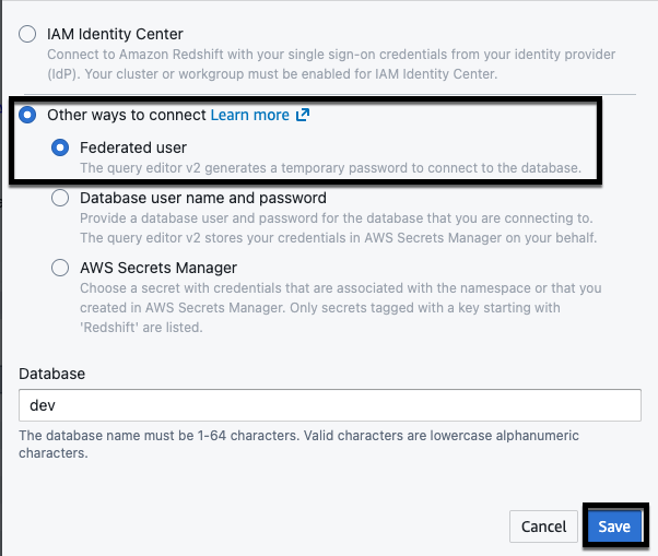
Secure credential management

For better security and maintainability, use JDBC or ODBC temporary AWS Identity and Access Management (IAM) credentials for database authentication. For details, see Connect to a cluster with Amazon Redshift RSQL.

Query logging and debugging

Debugging and troubleshooting SQL scripts can be challenging, especially when dealing with complex queries or error scenarios. To simplify this process, it’s recommended to enable query logging in RSQL scripts.

RSQL provides the echo-queries option, which prints the executed SQL queries along with their execution status. By invoking the RSQL client with this option, you can track the progress of your script and identify potential issues.

rsql --echo-queries -D testiam

Here testiam represents a DSN connection configured in odbc.ini with an IAM profile.

You can store these logs by redirecting the output when executing your RSQL script:

```
sh <path to RSQL file>/<RSQL file name>.sh  >  <log file name>.log
```

With query logging is enabled, you can examine the output and identify the specific query that caused an error or unexpected behavior. This information can be invaluable when troubleshooting and optimizing your RSQL scripts.

Error handling with incremental exit codes

Implement robust error handling using incremental exit codes to identify specific failure points. Proper error handling is crucial in a scripting environment, and RSQL is no exception. In BTEQ scripts, errors were typically handled by checking the error code and taking appropriate actions. However, in RSQL, the approach is slightly different. To help ensure robust error handling and straightforward troubleshooting, it’s recommended that you implement incremental exit codes at the end of each SQL operation.The incremental exit code approach works as follows:

After executing a SQL statement (such as SELECT, INSERT, UPDATE, and so on.), check the value of the :ERROR variable.
If the :ERROR variable is non-zero, it indicates that an error occurred during the execution of the SQL statement.
Print the error message, error code, and additional relevant information using RSQL commands such as \echo, \remark, and so on.
Exit the script with an appropriate exit code using the \exit command, where the exit code represents the specific operation that failed.

By using incremental exit codes, you can identify the point of failure within the script. This approach not only aids in troubleshooting but also allows for better integration with continuous integration and deployment (CI/CD) pipelines, where specific exit codes can trigger appropriate actions.

Example:

SELECT * FROM $STAGING_TABLE_SCHEMA.SAMPLE_TABLE;
\if :ERROR <> 0
      \echo 'Error occurred in executing the select operation on table $STAGING_TABLE_SCHEMA.SAMPLE_TABLE'
      \echo :ERRORCODE
      \remark :LAST_ERROR_MESSAGE
      \exit 1  -- Exit code 1 represents a failure in the SELECT operation
\else
      \echo 'Select statement completed successfully'
INSERT INTO $STAGING_TABLE_SCHEMA.ANOTHER_SAMPLE_TABLE 
SELECT * FROM $STAGING_TABLE_SCHEMA.SAMPLE_TABLE;
\if :ERROR <> 0
      \echo 'Error occurred in executing the insert operation on table $STAGING_TABLE_SCHEMA.SAMPLE_TABLE'
      \echo :ERRORCODE
      \remark :LAST_ERROR_MESSAGE
      \exit 2  -- Exit code 2 represents a failure in the INSERT operation
\else
      \echo 'Insert statement completed successfully'

In the preceding example, if the SELECT statement fails, the script will exit with an exit code of 1. If the INSERT statement fails, the script will exit with an exit code of 2. By using unique exit codes for different operations, you can quickly identify the point of failure and take appropriate actions.

Use query groups

When troubleshooting issues in your RSQL scripts, it can be helpful to identify the root cause by analyzing query logs. By using query groups, you can label a group of queries that are run during the same session, which can help pinpoint problematic queries in the logs.

To set a query group at the session level, you can use the following command:

set query_group to $QUERY_GROUP;

By setting a query group, queries executed within that session will be associated with the specified label. This technique can significantly aid in effective troubleshooting when you need to identify the root cause of an issue.

Use a search path

When creating an RSQL script that refers to tables from the same schema multiple times, you can simplify the script by setting a search path. By using a search path, you can directly reference table names without specifying the schema name in your queries (for example, SELECT, INSERT, and so on).

To set the search path at the session level, you can use the following command:

set search_path to $STAGING_TABLE_SCHEMA;

After setting the search path to $STAGING_TABLE_SCHEMA, you can refer to tables within that schema directly, without including the schema name.

For example:

SELECT * FROM STAGING_TABLE;

If you haven’t set a search path, you need to specify the schema name in the query, as shown in the following example:

SELECT * FROM $STAGING_TABLE_SCHEMA.STAGING_TABLE;

It’s recommended to use a fully qualified path for an object in an RSQL script, but adding the search path prevents abrupt execution failure because of not providing a fully qualified path.

Combine multiple UPDATE statements into a single INSERT

In BTEQ scripts, it might have multiple sequential UPDATE statements for the same table. However, this approach can be inefficient and lead to performance issues, especially when dealing with large datasets, because of I/O intensive operations.

To address this concern, it’s recommended to combine all or some of the UPDATE statements into a single INSERT statement. This can be achieved by creating a temporary table, converting the UPDATE statements into a LEFT JOIN with the staging table using a SELECT statement, and then inserting the temporary table data into the staging table.

Example:

The existing BTEQ SQLs in the following example first INSERT the data into staging_table from staging_table1 and then UPDATE the columns for inserted data if certain condition is satisfied:

Insert into SAMPLE_STAGING_TABLE_SCHEMA.staging_table select col1,col2,col3,col4,col5 from SAMPLE_STAGING_TABLE_SCHEMA.staging_table1 where col1=col2;

Update SAMPLE_STAGING_TABLE_SCHEMA.staging_table a from (select col1,col2 from SAMPLE_STAGING_TABLE_SCHEMA.staging_table2 where col1!=col2) b where a.col1=b.col1 set a.col2 =b.col2;
Update SAMPLE_STAGING_TABLE_SCHEMA.staging_table a from (select col3,col2 from SAMPLE_STAGING_TABLE_SCHEMA.staging_table2 where col3!=col1) c where a.col2=c.col2 set a.col3=c.col3;

Update SAMPLE_STAGING_TABLE_SCHEMA.staging_table where col4='no' set col4='yes';
Update SAMPLE_STAGING_TABLE_SCHEMA.staging_table where col1='zyx' set col1 ='nochange';

The following RSQL operation below achieves the same result by first loading the data into a staging table, then executing the UPDATE using a temporary table as an intermediate step and then completes UPDATE using a temporary table. After this, it will truncate staging_tables and insert temporary table staging_table_temp1 data into staging_table.

Insert into $STAGING_TABLE_SCHEMA.staging_table select col1,col2,col3,col4,col5 from $STAGING_TABLE_SCHEMA.staging_table1 where col1=col2;

\if :ERROR <> 0
      \echo 'Error occurred in executing the insert operation on table staging_table'
      \echo :ERRORCODE
      \remark :LAST_ERROR_MESSAGE
      \exit 1
\else
      \echo 'Insert statement completed successfully'

Create temporary table staging_table_temp1 (like $STAGING_TABLE_SCHEMA.staging_table including defaults);

\if :ERROR <> 0
      \echo 'Error occurred in creating the temporary table staging_table_temp1'
      \echo :ERRORCODE
      \remark :LAST_ERROR_MESSAGE
      \exit 2
\else
      \echo 'Temporary table created successfully'
Insert into staging_table_temp1
(
Col1,
Col2,
Col3,
Col4
)
select
case when col1='zyx' then 'nochange'
else a.col1
end as col1,
coalesce(b.col2,a.col2) as col2,
coalesce(c.col3,a.col3) as col3,
case when col4='no' then 'yes'
            else a.col4
end as col4
from $STAGING_TABLE_SCHEMA.staging_table a
left join (select col1,col2 from $STAGING_TABLE_SCHEMA.staging_table2 where col1!=col2) b
      on a.col1=b.col1
left join (select col3,col2 from $STAGING_TABLE_SCHEMA.staging_table2 where col3!=col1) c
      on a.col2=c.col2;
\if :ERROR <> 0
      \echo 'Error occurred in executing the insert operation on temporary table staging_table_temp1'
      \echo :ERRORCODE
      \remark :LAST_ERROR_MESSAGE
      \exit 3
\else
      \echo 'Insert statement completed successfully'
--Truncate table staging_table;
$STORED_PROCEDURE_SCHEMA.sp_truncate_table(‘$STAGING_TABLE_SCHEMA’,’staging_table’)

\if :ERROR <> 0
      \echo 'Error occurred in executing the Truncate operation on table $STAGING_TABLE_SCHEMA.staging_table'
      \echo :ERRORCODE
      \remark :LAST_ERROR_MESSAGE
      \exit 4
\else
      \echo 'Truncate statement completed successfully'

Insert into $STAGING_TABLE_SCHEMA.staging_table(col1,col2,col3,col4) select col1,col2,col3,col4 from staging_table_temp1;

\if :ERROR <> 0
      \echo 'Error occurred in executing the insert operation on table $STAGING_TABLE_SCHEMA.staging_table'
      \echo :ERRORCODE
      \remark :LAST_ERROR_MESSAGE
      \exit 5
\else
      \echo 'Insert statement completed successfully'

The following is an overview of the preceding logic:

Create a temporary table with the same structure as the staging table.
Execute a single INSERT statement that combines the logic of all the UPDATE statements from the BTEQ script. The INSERT statement uses a LEFT JOIN to merge data from the staging table and the staging_table2 table, applying the necessary transformations and conditions.
After inserting the data into the temporary table, truncate the staging table and insert the data from the temporary table into the staging table.

By consolidating multiple UPDATE statements into a single INSERT operation, you can improve the overall performance and efficiency of the script, especially when dealing with large datasets. This approach also promotes better code readability and maintainability.

Execution logs

Troubleshooting and debugging scripts can be a challenging task, especially when dealing with complex logic or error scenarios. To aid in this process, it’s recommended to generate execution logs for RSQL scripts.

Execution logs capture the output and error messages produced during the script’s execution, providing valuable information for identifying and resolving issues. These logs can be especially helpful when running scripts on remote servers or in automated environments, where direct access to the console output might be limited.

To generate execution logs, you can execute the RSQL script from the Amazon Elastic Compute Cloud (Amazon EC2) machine and redirect the output to a log file using the following command:

sample_rsql_script.sh > sample_rsql_script_$(date "+%Y.%m.%d-%H.%M.%S").log

The preceding command executes the RSQL script and redirects the output, including error messages or debugging information to the specified log file. It’s recommended to add a time parameter in the log file name to have distinct files for each run of RSQL script.

By maintaining execution logs, you can review the script’s behavior, track down errors, and gather relevant information for troubleshooting purposes. Additionally, these logs can be shared with teammates or support teams for collaborative debugging efforts.

Capture an audit parameter in the script

Audit parameters such as start time, end time, and the exit code of an RSQL script are important for troubleshooting, monitoring, and performance analysis. You can capture the start time at the beginning of your script and the end time and exit code after the script completes.

Here’s an example of how you can implement this:

# Capture start time
start=$(date +%s)
echo date : $(date)
echo Start Time : $(date +"%T.%N")
. <file_path>/rsql_parameters.
-- Your RSQL script logic goes here
      --End of the RSQL code	
-- Capture exit code and end time
	
rsqlexitcode=$?
echo Exited with error code $rsqlexitcode
echo End Time : $(date +"%T.%N")
end=$(date +%s)
exec=$(($end - $start))
echo Total Time Taken : $exec seconds

The preceding example captures the start time in start= $(date +%s). After the RSQL code is complete, it captures the exit code in rsqlexitcode=$? and the end time in end=$(date +%s).

Sample structure of the script

The following is a sample RSQL script that follows the best practices outlined in the preceding sections:

#bin/bash
#capturing start time of script execution
start=$(date +%s)
 
#Executing and setting rsql parameters script variables
. /<parameter script path>/rsql_parameters.sh
echo date : $(date)
echo Start Time : $(date +"%T.%N")
 
#Logging into Redshift cluster. Here credentials are retrieved from ODBC based temporary 
#IAM credentials which is discussed in Credentials Management section
rsql --echo-queries -D testiam < EOF 
\timing true
 
\echo '\n-----MAIN EXECUTION LOG STARTING HERE-----'
\echo '\n--JOB ${0:2} STARTING--'
 
/* Setting query group. Here $QUERY_GROUP retrieved from RSQL parameters file*/
SET query_group to '$QUERY_GROUP';
\if :ERROR <> 0
\echo 'Setting Query Group to $QUERY_GROUP failed '
\echo 'Error Code -'
\echo :ERRORCODE
\remark :LAST_ERROR_MESSAGE
\exit 1
\else
\remark '\n **** Setting Query Group to $QUERY_GROUP Successfully **** \n'
\endif
 
 
/*Setting search path to Staging table schema*/
SET SEARCH_PATH TO $STAGING_TABLE_SCHEMA, pg_catalog;
 
\if :ERROR <> 0
\echo 'SET SEARCH_PATH TO $STAGING_TABLE_SCHEMA, pg_catalog failed.'
\echo 'Error Code -'
\echo :ERRORCODE
\remark :LAST_ERROR_MESSAGE
\exit 2
\else
\remark '\n **** SET SEARCH_PATH TO $STAGING_TABLE_SCHEMA, pg_catalog executed Successfully **** \n'
\endif
/* Inserting initial data from staging_table1 into staging_table */
Insert into staging_table select col1,col2,col3,col4,col5 from staging_table1 where col1=col2;

\if :ERROR <> 0
      \echo 'Error occurred in executing the insert operation on table staging_table'
      \echo :ERRORCODE
      \remark :LAST_ERROR_MESSAGE
      \exit 3
\else
      \echo 'Insert statement completed successfully'

/* Creating temporary table for handling multiple updates using select statement*/
Create temporary table staging_table_temp1 (like $STAGING_TABLE_SCHEMA.staging_table including defaults);

\if :ERROR <> 0
      \echo 'Error occurred in creating the temporary table staging_table_temp1'
      \echo :ERRORCODE
      \remark :LAST_ERROR_MESSAGE
      \exit 4
\else
      \echo 'Temporary table created successfully'

/* Updates handling using insert and select statement*/

Insert into staging_table_temp1(Col1,Col2,Col3,Col4)
select
case when col1='zyx' then 'nochange' else a.col1 end as col1,
coalesce(b.col2,a.col2) as col2,
coalesce(c.col3,a.col3) as col3,
case when col4='no' then 'yes' else a.col4 end as col4
from $STAGING_TABLE_SCHEMA.staging_table a
left join (select col1,col2 from $STAGING_TABLE_SCHEMA.staging_table2 where col1!=col2) b 
      on a.col1=b.col1
left join (select col3,col2 from $STAGING_TABLE_SCHEMA.staging_table2 where col3!=col1) c
      on a.col2=c.col2;

\if :ERROR <> 0
      \echo 'Error occurred in executing the insert operation on temporary table staging_table_temp1'
      \echo :ERRORCODE
      \remark :LAST_ERROR_MESSAGE
      \exit 5
\else
      \echo 'Insert statement completed successfully'

/*In production, ETL user may not have truncate table permission therefore, to avoid permission issue we are using a stored procedure which can truncate required table by using provided schema name and table name. 
Note: You can create a stored procedure for truncating the tables and refer in all ETL RSQL script */

$STORED_PROCEDURE_SCHEMA.sp_truncate_table(‘$STAGING_TABLE_SCHEMA’,’staging_table’)
\if :ERROR <> 0
      \echo 'Error occurred in executing the Truncate operation on table $STAGING_TABLE_SCHEMA.staging_table'
      \echo :ERRORCODE
      \remark :LAST_ERROR_MESSAGE
      \exit 6
\else
      \echo 'Truncate statement completed successfully'

/* Inserting data from temporary table into staging table staging_table */

Insert into $STAGING_TABLE_SCHEMA.staging_table(col1,col2,col3,col4) select col1,col2,col3,col4 from staging_table_temp1;

\if :ERROR <> 0
      \echo 'Error occurred in executing the insert operation on table $STAGING_TABLE_SCHEMA.staging_table'
      \echo :ERRORCODE
      \remark :LAST_ERROR_MESSAGE
      \exit 7
\else
      \echo 'Insert statement completed successfully'

EOF

#Capture RSQL return code to exit the script with proper error code and message

rsqlexitcode=$?
echo Exited with error code $rsqlexitcode
echo End Time : $(date +"%T.%N")
end=$(date +%s)
exec=$(($end - $start))
echo Total Time Taken : $exec seconds

Conclusion

In this post, we’ve explored crucial best practices for migrating Teradata BTEQ scripts to Amazon Redshift RSQL. We’ve shown you essential techniques including parameter management, secure credential handling, comprehensive logging, and robust error handling with incremental exit codes. We’ve also discussed query optimization strategies and methods that you can use to improve data modification operations. By implementing these practices, you can create efficient, maintainable, and production-ready RSQL scripts that fully use the capabilities of Amazon Redshift. These approaches not only help ensure a successful migration, but also set the foundation for optimized performance and straightforward troubleshooting in your new Amazon Redshift environment.

To get started with your BTEQ to RSQL migration, explore these additional resources:

About the authors

Ankur Bhanawat is a Consultant with the Professional Services team at AWS based out of Pune, India. He’s an AWS certified professional in three areas and specialized in databases and serverless technologies. He has experience in designing, migrating, deploying, and optimizing workloads on the AWS Cloud.

Raj Patel is AWS Lead Consultant for Data Analytics solutions based out of India. He specializes in building and modernizing analytical solutions. His background is in data warehouse architecture, development, and administration. He has been in data and analytical field for over 14 years.

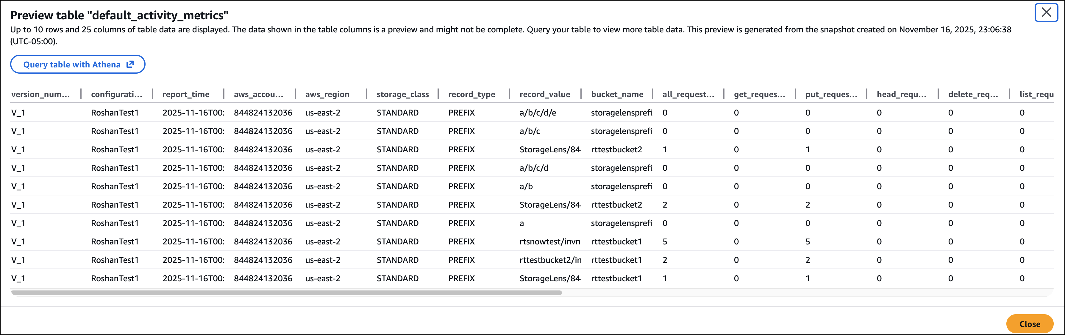
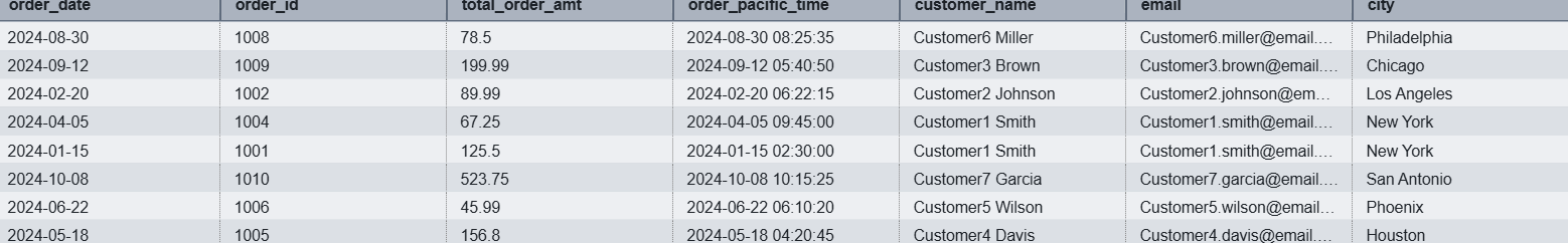
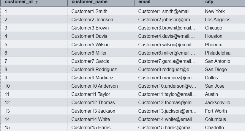
Amazon Redshift Serverless at 4 RPUs: High-value analytics at low cost

2025-08-22 Ricardo Serafim

Post Syndicated from Ricardo Serafim original https://aws.amazon.com/blogs/big-data/amazon-redshift-serverless-at-4-rpus-high-value-analytics-at-low-cost/

Organizations across industries struggle with the economics of data analytics. High entry costs, complex capacity planning, and unpredictable workload demands create barriers that prevent teams from accessing the insights they need. Small businesses abandon analytics initiatives due to prohibitive minimums, and enterprises overprovision resources for development environments, leading to inefficient spending.

Amazon Redshift Serverless now addresses these challenges with 4 RPU configurations, helping you get started with a lower base capacity that runs scalable analytics workloads beginning at $1.50 per hour. This new option transforms the economics of data analytics with the flexibility to scale up automatically based on workload demands. You only pay for the compute capacity you consume, calculated on a per-second basis.

With 64 GB of memory and support for up to 32 TB of managed storage, this lower entry point offering addresses several common customer needs, including development and test environments that maintain separate workloads at lower cost and production workloads with variable demand that need cost-effective scaling. The configuration is particularly useful for test and development environments, departmental data warehouses, periodic reporting workloads, gaming analytics, and data mesh architectures with unpredictable usage patterns. Organizations just starting with cloud analytics can use this low-cost option while getting access to enterprise features like automatic scaling, built-in security, and seamless data lake integration.In this post, we examine how this new sizing option makes Redshift Serverless accessible to smaller organizations while providing enterprises with cost-effective environments for development, testing, and variable workloads.

New 4 RPU minimum base capacity in Redshift Serverless

Redshift Serverless measures compute capacity using Redshift Processing Units (RPUs), where each RPU provides 16 GB of memory. With this new minimum base capacity, the 4 RPU configuration delivers a total of 64 GB of memory. It supports up to 32 TB of managed storage, with a maximum of 100 columns per table. The 4 RPU configuration is cost-efficient, and it’s designed for lighter workloads. When your workload requires additional resources, Redshift Serverless automatically scales up the compute capacity. After you have scaled beyond 4 RPUs, your data warehouse will continue using the higher RPU level to maintain consistent performance. This behavior provides workload stability while preserving the benefits of automatic scaling.

For workloads requiring more resources, such as tables with a large number of columns or higher concurrency requirements, you can choose higher base capacities ranging from 8 RPUs up to 1024 RPUs. This flexibility helps you start small and adjust your resources as your analytics requirements evolve.

Benefits of Redshift Serverless with 4 RPUs

This new feature offers the following benefits:

Cost-effective entry point – The new 4 RPU configuration is a low-cost option for cloud data warehousing, making enterprise-grade analytics accessible to organizations of various sizes, such as startups exploring their first data warehouse or established enterprises optimizing their analytics spending. For example, in the US East (N. Virginia) Region, the compute cost is $0.375 per RPU-hour. For a 4 RPU base capacity, this translates to $1.50 per hour of active workload time. Because you’re only charged when workloads are running, small-scale users can keep costs predictable and low. This configuration helps teams begin their analytics journey with minimal upfront commitment. Development teams can maintain dedicated environments for testing and experimentation without significant cost overhead.
Support for smaller datasets – With support for up to 32 TB of Redshift Managed Storage, the 4 RPU configuration is well-suited for smaller data warehouses. It can handle datasets ranging from a few gigabytes to tens of terabytes, making it ideal for startups, small businesses, or departments with limited data volumes.
Seamless integration with the AWS ecosystem – The 4 RPU configuration integrates seamlessly with other AWS services, such as Amazon Simple Storage Service (Amazon S3) for data lakes, AWS Glue for ETL (extract, transform, and load), and Amazon QuickSight for visualization. This makes it straightforward to build end-to-end analytics pipelines, even for smaller-scale projects. Additionally, Redshift data lake queries on external Amazon S3 data are included in the RPU billing, simplifying cost management.
Use case flexibility – The 4 RPU configuration proves valuable across numerous analytics scenarios. Development and testing environments benefit from cost-effective isolation, and departmental data warehouses can start small and scale as needed. Organizations running periodic reporting workloads or proof-of-concept projects can optimize costs by paying only for actual usage. Even small to medium-sized production workloads can use this configuration effectively.

Regardless of the use case, you can benefit from the full feature set of Redshift Serverless, including built-in security, data lake integration, and automated maintenance.

Use cases for Redshift Serverless with 4 RPU workgroups

The 4 RPU configuration is tailored for scenarios where lightweight compute resources suffice. The following are some practical use cases:

Small business analytics – Small businesses with limited data (less than 32 GB) can analyze sales, customer behavior, or operational metrics with cost-effective data warehouses. Running 10–20 daily ETL queries and occasional one-time queries remains cost-effective at this capacity.
Development and testing environments – The configuration is well-suited for development and test environments where full production resources aren’t needed. Data engineers can experiment with Redshift Serverless, prototype queries, or build proof-of-concept solutions without committing to higher RPU capacities. The 4 RPU configuration lowers the cost of continuous integration and delivery (CI/CD) testing of data pipelines. Teams can run automated integration tests and schema validations in isolated environments that mirror production systems while optimizing costs through per-second billing.
Analytics for startups – Startups can build robust product analytics capabilities without significant upfront investment. Teams can track customer behavior, feature adoption, and KPIs using familiar SQL queries, then connect business intelligence (BI) tools like Quicksight or Tableau for lightweight dashboarding.
Training and experimentation – Organizations can create dedicated sandbox environments for data analysts’ onboarding and experimentation with minimal budget impact. These environments are perfect for exploring analytics powered by large language models (LLMs), semantic layer development, or generative AI applications.
Data quality workflows – The feature efficiently supports scheduled jobs for data quality validation, checking data freshness, integrity, and conformance without dedicating high-capacity environments to routine QA tasks.
Enterprise team enablement – Large organizations can implement decentralized data warehousing strategies. Each department can operate its data warehouse aligned with specific needs and budgets, enabling department-level chargeback models.
Environment isolation – Organizations can create dedicated workgroups per environment (development, test, QA, UAT), providing complete isolation without sharing compute resources or risking cross-environment interference.
Data mesh architecture – Domain teams can operate independently while maintaining cost-efficiency. Each domain runs its workgroup for lightweight transformations, domain-specific marts, and KPI calculations. It offers a flexible sizing option in a data mesh architecture.
Event-driven analytics – Well-suited for short-lived or event-triggered analytics tasks. Organizations can programmatically create workgroups through APIs for A/B test analysis, campaign performance summaries, or machine learning (ML) pipeline validation.
Low-volume one-time reporting – Organizations with infrequent or lightweight reporting needs, such as monthly financial summaries or dashboard refreshes, can use 4 RPUs to minimize costs while maintaining performance.

Cost considerations and best practices

Although the 4 RPU configuration is cost-effective, there are a few considerations to keep in mind to optimize expenses:

Billing – Redshift Serverless bills on a per-second basis with a 60-second minimum per query. For very short queries (such as subsecond), this can inflate costs. To mitigate this, batch queries where possible to maximize resource utilization within the 60-second window. For more information, see Amazon Redshift pricing.
Set usage limits – Use the Redshift Serverless console to set maximum RPU-hour limits (daily, weekly, or monthly) to prevent unexpected costs. You can configure alerts or automatically turn off queries when limits are reached. To learn more, see Setting usage limits, including setting RPU limits.
Monitor with system views – Query the SYS_SERVERLESS_USAGE system table to track RPU consumption and estimate query costs. For example, you can calculate daily costs by aggregating charged seconds and multiplying by the RPU rate.
Close transactions – Make sure transactions are explicitly closed (using COMMIT or ROLLBACK) to avoid idle sessions consuming RPUs, which can lead to unnecessary charges.

The following is a practical example for a 4 RPU workgroup in US East (N. Virginia) at $0.375/RPU-hour for a scenario of a 10-minute query running daily: This is compute costs only. Primary storage capacity is billed as Redshift Managed Storage (RMS).

Workload duration: 10 minutes (600 seconds)
Cost: (600 seconds / 3600 seconds) × 4 RPUs × $0.375 = $0.25
Monthly cost (30 days): $0.25 × 30 = $7.50

Performance considerations

Although the 4 RPU configuration is cost-efficient, it’s designed for lighter workloads. For complex queries or datasets exceeding 32 TB, you must set up 8 RPUs to 24 RPUs to support up to 128 TB of storage. For more than 128 TB, you need 32 RPUs or more. If query performance is a priority, consider increasing the base capacity or enabling AI-driven scaling and optimization to optimize resources dynamically. Benchmark tests suggest that higher RPUs (such as 32 RPUs) significantly improve performance for complex queries. However, for simpler tasks, 4 RPUs deliver adequate throughput.

To monitor performance, use the Redshift Serverless console or CloudWatch metrics like ComputeCapacity and ComputeSeconds. The SYS_QUERY_HISTORY table can also help analyze query runtimes and identify bottlenecks.

Conclusion

Redshift Serverless with 4 RPU represents a significant step forward in making enterprise-grade analytics cheaper and accessible to organizations of different sizes, such as a startup building its first analytics system, a development team looking to optimize testing environments, or an enterprise implementing a data mesh architecture. This new configuration combines the power and flexibility of Redshift Serverless with a cost-effective entry point, so teams can start small and scale seamlessly as their needs grow. The ability to begin with minimal commitment while maintaining access to advanced features like automatic scaling, built-in security, and seamless data lake integration makes this a compelling option for modern data analytics workloads. Combined with pay-per-second billing and intelligent resource management, Redshift Serverless with 4 RPU delivers the ideal balance of cost-efficiency and performance.

To get started with cost-effective analytics, visit the AWS Management Console to create your Redshift Serverless workgroup with 4 RPUs. For more information, refer to the Amazon Redshift Serverless Management Guide or Amazon Redshift best practices. Plan your analytics budget effectively using the AWS Pricing Calculator to estimate costs based on your specific workload patterns, or contact your AWS account team to discuss your particular use case.

About the authors

Build data pipelines with dbt in Amazon Redshift using Amazon MWAA and Cosmos

2025-08-13 Cindy Li

Post Syndicated from Cindy Li original https://aws.amazon.com/blogs/big-data/build-data-pipelines-with-dbt-in-amazon-redshift-using-amazon-mwaa-and-cosmos/

Effective collaboration and scalability are essential for building efficient data pipelines. However, data modeling teams often face challenges with complex extract, transform, and load (ETL) tools, requiring programming expertise and a deep understanding of infrastructure. This complexity can lead to operational inefficiencies and challenges in maintaining data quality at scale.

dbt addresses these challenges by providing a simpler approach where data teams can build robust data models using SQL, a language they’re already familiar with. When integrated with modern development practices, dbt projects can use version control for collaboration, incorporate testing for data quality, and utilize reusable components through macros. dbt also automatically manages dependencies, making sure data transformations execute in the correct sequence.

In this post, we explore a streamlined, configuration-driven approach to orchestrate dbt Core jobs using Amazon Managed Workflows for Apache Airflow (Amazon MWAA) and Cosmos, an open source package. These jobs run transformations on Amazon Redshift, a fully managed data warehouse that enables fast, scalable analytics using standard SQL. With this setup, teams can collaborate effectively while maintaining data quality, operational efficiency, and observability. Key steps covered include:

Creating a sample dbt project
Enabling auditing within the dbt project to capture runtime metrics for each model
Creating a GitHub Actions workflow to automate deployments
Setting up Amazon Simple Notification Service (Amazon SNS) to proactively alert on failures

These enhancements enable model-level auditing, automated deployments, and real-time failure alerts. By the end of this post, you will have a practical and scalable framework for running dbt Core jobs with Cosmos on Amazon MWAA, so your team can ship reliable data workflows faster.

Solution overview

The following diagram illustrates the solution architecture.

The workflow contains the following steps:

Analytics engineers manage their dbt project in their version control tool. In this post, we use GitHub as an example.
We configure an Apache Airflow Directed Acyclic Graph (DAG) to use the Cosmos library to create an Airflow task group that contains all the dbt models as part of the dbt project.
We use a GitHub Actions workflow to sync the dbt project files and the DAG to an Amazon Simple Storage Service (Amazon S3) bucket.
During the DAG run, dbt converts the models, tests, and macros to Amazon Redshift SQL statements, which run directly on the Redshift cluster.
If a task in the DAG fails, the DAG invokes an AWS Lambda function to send out a notification using Amazon SNS.

Prerequisites

You must have the following prerequisites:

A Redshift provisioned cluster or a Redshift serverless workgroup. For creation instructions, refer to the Amazon Redshift Management Guide.
An S3 bucket to store dbt project files and DAGs.
An Amazon MWAA environment. For creation instructions, refer to Create an Amazon MWAA Environment.
Network connectivity from Amazon MWAA to Amazon Redshift. Deploy Amazon MWAA and your Redshift cluster in the same virtual private cloud (VPC). Add an Amazon MWAA security group as a source for the Redshift security group inbound rule.
An AWS Identity and Access Management (IAM) role to connect GitHub Actions to actions in AWS. For creation instructions, refer to Use IAM roles to connect GitHub Actions to actions in AWS and Security best practices in IAM.

Create a dbt project

A dbt project is structured to facilitate modular, scalable, and maintainable data transformations. The following code is a sample dbt project structure that this post will follow:

MY_SAMPLE_DBT_PROJECT
├── .github
│   └── workflows
│       └── publish_assets.yml
└── src
    ├── dags
    │   └── dbt_sample_dag.py
    └── my_sample_dbt_project
        ├── macros
        ├── models
        └── dbt_project.yml

dbt uses the following YAML files:

dbt_project.yml – Serves as the main configuration for your project. Objects in this project will inherit settings defined here unless overridden at the model level. For example:

# Name your project! Project names should contain only lowercase characters
# and underscores. 
name: 'my_sample_dbt_project'
version: '1.0.0'

# These configurations specify where dbt should look for different types of files.
# The `model-paths` config, for example, states that models in this project can be
# found in the "models/" directory. 
model-paths: ["models"]
macro-paths: ["macros"]

# Configuring models
# Full documentation: https://docs.getdbt.com/docs/configuring-models
# In this example config, we tell dbt to build models in the example/
# directory as views. These settings can be overridden in the individual model
# files using the `{{ config(...) }}` macro.
models:
  my_sample_dbt_project:
    # Config indicated by + and applies to files under models/example/
    example:
      +materialized: view
      
on-run-end:
# add run results to audit table 
  - "{{ log_audit_table(results) }}"

sources.yml – Defines the external data sources that your dbt models will reference. For example:

sources:
  - name: sample_source
    database: sample_database
    schema: sample_schema
    tables:
      - name: sample_table

schema.yml – Outlines the schema of your models and data quality tests. In the following example, we have defined two columns, full_name for the model model1 and sales_id for model2. We have declared them as the primary key and defined data quality tests to check if the two columns are unique and not null.

version: 2

models:
  - name: model1
    config: 
      contract: {enforced: true}

    columns:
      - name: full_name
        data_type: varchar(100)
        constraints:
          - type: primary_key
        tests:
          - unique
          - not_null

  - name: model2
    config: 
      contract: {enforced: true}

    columns:
      - name: sales_id
        data_type: varchar(100)
        constraints:
          - type: primary_key
        tests:
          - unique
          - not_null

Enable auditing within dbt project

Enabling auditing within your dbt project is crucial for facilitating transparency, traceability, and operational oversight across your data pipeline. You can capture run metrics at the model level for each execution in an audit table. By capturing detailed run metrics such as load identifier, runtime, and number of rows affected, teams can systematically monitor the health and performance of each load, quickly identify issues, and trace changes back to specific runs.

The audit table consists of the following attributes:

load_id – An identifier for each model run executed as part of the load
database_name – The name of the database within which data is being loaded
schema_name – The name of the schema within which data is being loaded
name – The name of the object within which data is being loaded
resource_type – The type of object to which data is being loaded
execution_time – The time duration taken for each dbt model to complete execution as part of each load
rows_affected – The number of rows affected in the dbt model as part of the load

Complete the following steps to enable auditing within your dbt project:

Navigate to the models directory (src/my_sample_dbt_project/models) and create the audit_table.sql model file:

{%- set run_date = "CURRENT_DATE" -%}
{{
    config(
        materialized='incremental',
        incremental_strategy='append',
        tags=["audit"]
    )
}}

with empty_table as (
    select
        'test_load_id'::varchar(200) as load_id,
        'test_invocation_id'::varchar(200) as invocation_id,
        'test_database_name'::varchar(200) as database_name,
        'test_schema_name'::varchar(200) as schema_name,
        'test_model_name'::varchar(200) as name,
        'test_resource_type'::varchar(200) as resource_type,
        'test_status'::varchar(200) as status,
        cast('12122012' as float) as execution_time,
        cast('100' as int) as rows_affected,
        {{run_date}} as model_execution_date
)

select * from empty_table
-- This is a filter so we will never actually insert these values
where 1 = 0

Navigate to the macros directory (src/my_sample_dbt_project/macros) and create the parse_dbt_results.sql macro file:

{% macro parse_dbt_results(results) %}
    -- Create a list of parsed results
    {%- set parsed_results = [] %}
    -- Flatten results and add to list
    {% for run_result in results %}
        -- Convert the run result object to a simple dictionary
        {% set run_result_dict = run_result.to_dict() %}
        -- Get the underlying dbt graph node that was executed
        {% set node = run_result_dict.get('node') %}
        {% set rows_affected = run_result_dict.get(
        'adapter_response', {}).get('rows_affected', 0) %}
        {%- if not rows_affected -%}
            {% set rows_affected = 0 %}
        {%- endif -%}
        {% set parsed_result_dict = {
                'load_id': invocation_id ~ '.' ~ node.get('unique_id'),
                'invocation_id': invocation_id,
                'database_name': node.get('database'),
                'schema_name': node.get('schema'),
                'name': node.get('name'),
                'resource_type': node.get('resource_type'),
                'status': run_result_dict.get('status'),
                'execution_time': run_result_dict.get('execution_time'),
                'rows_affected': rows_affected
                }%}
        {% do parsed_results.append(parsed_result_dict) %}
    {% endfor %}
    {{ return(parsed_results) }}
{% endmacro %}

Navigate to the macros directory (src/my_sample_dbt_project/macros) and create the log_audit_table.sql macro file:

{% macro log_audit_table(results) %}
    -- depends_on: {{ ref('audit_table') }}
    {%- if execute -%}
        {{ print("Running log_audit_table Macro") }}
        {%- set run_date = "CURRENT_DATE" -%}
        {%- set parsed_results = parse_dbt_results(results) -%}
        {%- if parsed_results | length  > 0 -%}
            {% set allowed_columns = ['load_id', 'invocation_id', 'database_name', 
            'schema_name', 'name', 'resource_type', 'status', 'execution_time', 
            'rows_affected', 'model_execution_date'] -%}
            {% set insert_dbt_results_query -%}
                insert into {{ ref('audit_table') }}
                    (
                        load_id,
                        invocation_id,
                        database_name,
                        schema_name,
                        name,
                        resource_type,
                        status,
                        execution_time,
                        rows_affected,
                        model_execution_date
                ) values
                    {%- for parsed_result_dict in parsed_results -%}
                        (
                            {%- for column, value in parsed_result_dict.items() %}
                                {% if column not in allowed_columns %}
                                    {{ exceptions.raise_compiler_error("Invalid
                                     column") }}
                                {% endif %}
                                {% set sanitized_value = value | replace("'", "''") %}
                                '{{ sanitized_value }}'
                                {%- if not loop.last %}, {% endif %}
                            {%- endfor -%}
                        )
                        {%- if not loop.last %}, {% endif %}
                    {%- endfor -%}
            {%- endset -%}
            {%- do run_query(insert_dbt_results_query) -%}
        {%- endif -%}
    {%- endif -%}
    {{ return ('') }}
{% endmacro %}

Append the following lines to the dbt_project.yml file:

on-run-end:
  - "{{ log_audit_table(results) }}"

Create a GitHub Actions workflow

This step is optional. If you prefer, you can skip it and instead upload your files directly to your S3 bucket.

The following GitHub Actions workflow automates the deployment of dbt project files and DAG file to Amazon S3. Replace the placeholders {s3_bucket_name}, {account_id}, {role_name}, and {region} with your S3 bucket name, account ID, IAM role name, and AWS Region in the workflow file.

To enhance security, it’s recommended to use OpenID Connect (OIDC) for authentication with IAM roles in GitHub Actions instead of relying on long-lived access keys.

name: Sync dbt Project with S3

on:
  workflow_dispatch:
  push:
    branches: [ main ]
    paths:
      - "src/**"

permissions:
  id-token: write   # This is required for requesting the JWT
  contents: read    # This is required for actions/checkout
  pull-requests: write

jobs:
  sync-dev:
    runs-on: ubuntu-latest
    environment: dev
    defaults:
      run:
        shell: bash
    steps:
      - uses: actions/checkout@v4
      - name: Assume AWS IAM Role
        uses: aws-actions/[email protected]
        with:
          aws-region: {region}
          role-to-assume: arn:aws:iam::{account_id}:role/{role_name}
          role-session-name: my_sample_dbt_project_${{ github.run_id }}
          role-duration-seconds: 3600 # 1 hour

      - run: aws sts get-caller-identity

      - name: Sync dbt Model files
        id: dbt_project_files
        working-directory: src/my_sample_dbt_project
        run: aws s3 sync . s3://{s3_bucket_name}/dags/dbt/my_sample_dbt_project 
        --delete
        continue-on-error: false

      - name: Sync DAG files
        id: dag_file
        working-directory: src/dags
        run: aws s3 sync . s3://{s3_bucket_name}/dags

GitHub has the following security requirements:

Branch protection rules – Before proceeding with the GitHub Actions workflow, make sure branch protection rules are in place. These rules enforce required status checks before merging code into protected branches (such as main).
Code review guidelines – Implement code review processes to make sure changes undergo review. This can include requiring at least one approving review before code is merged into the protected branch.
Incorporate security scanning tools – This can help detect vulnerabilities in your repository.

Make sure you are also adhering to dbt-specific security best practices:

Pay attention to dbt macros with variables and validate their inputs.
When adding new packages to your dbt project, evaluate their security, compatibility, and maintenance status to make sure they don’t introduce vulnerabilities or conflicts into your project.
Review dynamically generated SQL to safeguard against issues like SQL injection.

Update the Amazon MWAA instance

Complete the following steps to update the Amazon MWAA instance:

Install the Cosmos library on Amazon MWAA by adding astronomer-cosmos in the requirements.txt file. Make sure to check for version compatibility for Amazon MWAA and the Cosmos library.
Add the following entries in your startup.sh script:
1. In the following code, DBT_VENV_PATH specifies the location where the Python virtual environment for dbt will be created. DBT_PROJECT_PATH points to the location of your dbt project inside Amazon MWAA.
```
#!/bin/sh
export DBT_VENV_PATH="${AIRFLOW_HOME}/dbt_venv"
export DBT_PROJECT_PATH="${AIRFLOW_HOME}/dags/dbt"
```
2. The following code creates a Python virtual environment at the path ${DBT_VENV_PATH} and installs the dbt-redshift adapter to run dbt transformations on Amazon Redshift:
```
python3 -m venv "${DBT_VENV_PATH}"
${DBT_VENV_PATH}/bin/pip install dbt-redshift
```

Create a dbt user in Amazon Redshift and store credentials

To create dbt models in Amazon Redshift, you must set up a native Redshift user with the necessary permissions to access source tables and create new tables. It is essential to create separate database users with minimal permissions to follow the principle of least privilege. The dbt user should not be granted admin privileges, instead, it should only have access to the specific schemas required for its tasks.

Complete the following steps:

Open the Amazon Redshift console and connect as an admin (for more details, refer to Connecting to an Amazon Redshift database).
Run the following command in the query editor v2 to create a native user, and note down the values for dbt_user_name and password_value:
```
create user {dbt_user_name} password 'sha256|{password_value}';
```
Run the following commands in the query editor v2 to grant permissions to the native user:
1. Connect to the database where you want to source tables from and run the following commands:
```
grant usage on schema {schema_name} to {dbt_user_name};
grant select on all tables in schema {schema_name} to {dbt_user_name};
```
2. To allow the user to create tables within a schema, run the following command:
```
grant create on schema {schema_name} to {dbt_user_name};
```
Optionally, create a secret in AWS Secrets Manager and store the values for dbt_user_name and password_value from the previous step as plaintext:

{
    "username":"dbt_user_name",
    "password":"password_value"
}

Creating a Secrets Manager entry is optional, but recommended for securely storing your credentials instead of hardcoding them. To learn more, refer to AWS Secrets Manager best practices.

Create a Redshift connection in Amazon MWAA

We create one Redshift connection in Amazon MWAA for each Redshift database, making sure that each data pipeline (DAG) can only access one database. This approach provides distinct access controls for each pipeline, helping prevent unauthorized access to data. Complete the following steps:

Log in to the Amazon MWAA UI.
On the Admin menu, choose Connections.
Choose Add a new record.
For Connection Id, enter a name for this connection.
For Connection Type, choose Amazon Redshift.
For Host, enter the endpoint of the Redshift cluster without the port and database name (for example, redshift-cluster-1.xxxxxx.us-east-1.redshift.amazonaws.com).
For Database, enter the database of the Redshift cluster.
For Port, enter the port of the Redshift cluster.

Set up an SNS notification

Setting up SNS notifications is optional, but they can be a useful enhancement to receive alerts on failures. Complete the following steps:

Create an SNS topic.
Create a subscription to the SNS topic.
Create a Lambda function with the Python runtime.
Modify the function code in your Lambda function, and replace {topic_arn} with your SNS topic Amazon Resource Name (ARN):

import json

sns_client = boto3.client('sns')

def lambda_handler(event, context):
     try:
        # Extract DAG name from event
        failed_dag = event['dag_name']
        
        # Send notification 
        sns_client.publish(
            TopicArn={topic_arn}, 
            Subject="Data modelling dags - WARNING", 
            Message=json.dumps({'default': json.dumps(f"Data modelling DAG - 
            {failed_dag} has failed, please inform the data modelling team")}),
            MessageStructure='json'
        )
        
    except KeyError as e:
        # Handle missing 'dag_name' in the event
        logger.error(f"KeyError: invalid payload - dag_name not present")

Configure a DAG

The following sample DAG orchestrates a dbt workflow for processing and auditing data models in Amazon Redshift. It retrieves credentials from Secrets Manager, runs dbt tasks in a virtual environment, and sends an SNS notification if a failure occurs. The workflow consists of the following steps:

It starts with the audit_dbt_task task group, which creates the audit model.
The transform_data task group executes the other dbt models, excluding the audit-tagged one. Inside the transform_data group, there are two dbt models, model1 and model2, and each is followed by a corresponding test task that runs data quality tests defined in the schema.yml file.
To properly detect and handle failures, the DAG includes a dbt_check Python task that runs a custom function, check_dbt_failures. This is important because when using DbtTaskGroup, individual model-level failures inside the group don’t automatically propagate to the task group level. As a result, downstream tasks (such as the Lambda operator sns_notification_for_failure) configured with trigger_rule='one_failed' will not be triggered unless a failure is explicitly raised.

The check_dbt_failures function addresses this by inspecting the results of each dbt model and test, and raising an AirflowException if a failure is found. When an AirflowException is raised, the sns_notification_for_failure task is triggered.

If a failure occurs, the sns_notification_for_failure task invokes a Lambda function to send an SNS notification. If no failures are detected, this task is skipped.

The following diagram illustrates this workflow.

Configure DAG variables

To customize this DAG for your environment, configure the following variables:

project_name – Make sure the project_name matches the S3 prefix of your dbt project
secret_name – Provide the name of the secret that stores dbt user credentials
target_database and target_schema – Update these variables to reflect where you want to land your dbt models in Amazon Redshift
redshift_connection_id – Set this to match the connection configured in Amazon MWAA for this Redshift database
sns_lambda_function_name – Provide the Lambda function name to send SNS notifications
dag_name – Provide the DAG name that will be passed to the SNS notification Lambda function

import os
import json
import boto3
from airflow import DAG
from cosmos import (
    DbtTaskGroup, ProfileConfig, ProjectConfig,
    ExecutionConfig, RenderConfig
)
from cosmos.constants import ExecutionMode, LoadMode
from cosmos.profiles import RedshiftUserPasswordProfileMapping
from pendulum import datetime
from airflow.operators.python_operator import PythonOperator
from airflow.providers.amazon.aws.operators.lambda_function import (
    LambdaInvokeFunctionOperator
)
from airflow.exceptions import AirflowException

# project name - should match the s3 prefix of your dbt project
project_name = "my_sample_dbt_project"
# name of the secret that stores dbt user credentials 
secret_name = "dbt_user_credentials_secret"
# target database to land dbt models
target_database = "sample_database"
# target schema to land dbt models
target_schema = "sample_schema"
# Redshift connection name from MWAA
redshift_connection_id = "my_sample_dbt_project_connection"
# sns lambda function name
sns_lambda_function_name = "sns_notification"
# dag name - this will be passed to SNS for notification
payload = json.dumps({
            "dag_name": "my_sample_dbt_project_dag"
        })

Incorporate DAG components

After setting the variables, you can now incorporate the following components to complete the DAG.

Secrets Manager

The DAG retrieves dbt user credentials from Secrets Manager:

sm_client = boto3.client('secretsmanager')

def get_secret(secret_name):
    try:
        get_secret_value_response = sm_client.get_secret_value(SecretId=secret_name)
        return json.loads(get_secret_value_response["SecretString"])
    except Exception as e:
        raise

secret_value = get_secret(secret_name)
username = secret_value["username"]
password = secret_value["password"]

Redshift connection configuration

It uses RedshiftUserPasswordProfileMapping to authenticate:

profile_config = ProfileConfig(
    profile_name="redshift",
    target_name=target_database,
    profile_mapping=RedshiftUserPasswordProfileMapping(
        conn_id=redshift_connection_id,
        profile_args={"schema": target_schema,
                      "user": username, "password": password}
    ),
)

dbt execution setup

This code contains the following variables:

dbt executable path – Uses a virtual environment
dbt project path – Is located in the environment variable DBT_PROJECT_PATH under your project

execution_config = ExecutionConfig(
    dbt_executable_path=f"{os.environ['DBT_VENV_PATH']}/bin/dbt",
    execution_mode=ExecutionMode.VIRTUALENV,
)

project_config = ProjectConfig(
    dbt_project_path=f"{os.environ['DBT_PROJECT_PATH']}/{project_name}",
)

Tasks and execution flow

This step includes the following components:

Audit dbt task group (audit_dbt_task) – Runs the dbt model tagged with audit
dbt task group (transform_data) – Runs the dbt models tagged with operations, excluding the audit model

In dbt, tags are labels that you can assign to models, tests, seeds, and other dbt resources to organize and selectively run subsets of your dbt project. In your render_config, you have exclude=["tag:audit"]. This means dbt will exclude models that have the tag audit, because the audit model runs separately.

Failure check (dbt_check) – Checks for dbt model failures, raises an AirflowException if upstream dbt tasks fail
SNS notification on failure (sns_notification_for_failure) – Invokes a Lambda function to send an SNS notification upon a dbt task failure (for example, a dbt model in the task group)

def check_dbt_failures(**kwargs):
    if kwargs['ti'].state == 'failed':
        raise AirflowException('Failure in dbt task group')

with DAG(
    dag_id="my_sample_dbt_project_dag",
    start_date=datetime(2025, 4, 2),
    schedule_interval="@daily",
    catchup=False,
    tags=["dbt"]
):

    audit_dbt_task = DbtTaskGroup(
        group_id="audit_dbt_task",
        execution_config=execution_config,
        profile_config=profile_config,
        project_config=project_config,
        operator_args={
            "install_deps": True,
        },
        render_config= RenderConfig(
            select=["tag:audit"],
            load_method=LoadMode.DBT_LS
        )
    )

    transform_data = DbtTaskGroup(
        group_id="transform_data",
        execution_config=execution_config,
        profile_config=profile_config,
        project_config=project_config,
        operator_args={
            "install_deps": True,
            # install necessary dependencies before running dbt command
        },
        render_config= RenderConfig(
            exclude=["tag:audit"],
            load_method=LoadMode.DBT_LS
        )
    )

    dbt_check = PythonOperator(
        task_id='dbt_check', 
        python_callable=check_dbt_failures,
        provide_context=True,
    )

    sns_notification_for_failure = LambdaInvokeFunctionOperator(
        task_id="sns_notification_for_failure",
        function_name=sns_lambda_function_name,
        payload=payload,
        trigger_rule='one_failed'
    )

    audit_dbt_task >> transform_data >> dbt_check >> sns_notification_for_failure

The sample dbt orchestrates a dbt workflow in Amazon Redshift, starting with an audit task and followed by a task group that processes data models. It includes a failure handling mechanism that checks for failures and raises an exception to trigger an SNS notification using Lambda if a failure occurs. If no failures are detected, the SNS notification task is skipped.

Clean up

If you no longer need the resources you created, delete them to avoid additional charges. This includes the following:

Amazon MWAA environment
S3 bucket
IAM role
Redshift cluster or serverless workgroup
Secrets Manager secret
SNS topic
Lambda function

Conclusion

By integrating dbt with Amazon Redshift and orchestrating workflows using Amazon MWAA and the Cosmos library, you can simplify data transformation workflows while maintaining robust engineering practices. The sample dbt project structure, combined with automated deployments through GitHub Actions and proactive monitoring using Amazon SNS, provides a foundation for building reliable data pipelines. The addition of audit logging facilitates transparency across your transformations, so teams can maintain high data quality standards.

You can use this solution as a starting point for your own dbt implementation on Amazon MWAA. The approach we outlined emphasizes SQL-based transformations while incorporating essential operational capabilities like deployment automation and failure alerting. Get started by adapting the configuration to your environment, and build upon these practices as your data needs evolve.

For more resources, refer to Manage data transformations with dbt in Amazon Redshift and Redshift setup.

About the authors

Cindy Li is an Associate Cloud Architect at AWS Professional Services, specialising in Data Analytics. Cindy works with customers to design and implement scalable data analytics solutions on AWS. When Cindy is not diving into tech, you can find her out on walks with her playful toy poodle Mocha.

Akhil B is a Data Analytics Consultant at AWS Professional Services, specializing in cloud-based data solutions. He partners with customers to design and implement scalable data analytics platforms, helping organizations transform their traditional data infrastructure into modern, cloud-based solutions on AWS. His expertise helps organizations optimize their data ecosystems and maximize business value through modern analytics capabilities.

Joao Palma is a Senior Data Architect at Amazon Web Services, where he partners with enterprise customers to design and implement comprehensive data platform solutions. He specializes in helping organizations transform their data into strategic business assets and enabling data-driven decision making.

Harshana Nanayakkara is a Delivery Consultant at AWS Professional Services, where he helps customers tackle complex business challenges using AWS Cloud technology. He specializes in data and analytics, data governance, and AI/ML implementations.

Near real-time streaming analytics on protobuf with Amazon Redshift

2025-08-04 Konstantinos Tzouvanas

Post Syndicated from Konstantinos Tzouvanas original https://aws.amazon.com/blogs/big-data/near-real-time-streaming-analytics-on-protobuf-with-amazon-redshift/

Organizations must often deal with a vast array of data formats and sources in their data analytics workloads. This range of data types, such as structured relational data, semi-structured formats like JSON and XML and even binary formats like Protobuf and Avro, has presented new challenges for companies looking to extract valuable insights.

Protocol Buffers (protobuf) has gained significant traction in industries that require efficient data serialization and transmission, particularly in streaming data scenarios. Protobuf’s compact binary representation, language-agnostic nature, and strong typing make it an attractive choice for companies in sectors such as finance, gaming, telecommunications, and ecommerce, where high-throughput and low-latency data processing is crucial.

Although protobuf offers advantages in efficient data serialization and transmission, its binary nature poses challenges when it comes to analytics use cases. Unlike formats like JSON or XML, which can be directly queried and analyzed, protobuf data requires an additional deserialization step to convert it from its compact binary format into a structure suitable for processing and analysis. This extra conversion step introduces complexity into data analytics pipelines and tools. It can potentially slow down data exploration and analysis, especially in scenarios where near real-time insights are crucial.

In this post, we explore an end-to-end analytics workload for streaming protobuf data, by showcasing how to handle these data streams with Amazon Redshift Streaming Ingestion, deserializing and processing them using AWS Lambda functions, so that the incoming streams are immediately available for querying and analytical processing on Amazon Redshift.

The solution provides a solid foundation for handling protobuf data in Amazon Redshift. You can further enhance the architecture to support schema evolution by incorporating AWS Glue Schema Registry. By integrating the AWS Glue Schema Registry, you can make sure your Lambda function uses the latest schema version for deserialization, even as your data structure changes over time. However, for the purpose of this post and to maintain simplicity, we focus on demonstrating how to invoke Lambda from Amazon Redshift to convert protobuf messages to JSON format, which serves as a solid foundation for handling binary data in near real-time analytics scenarios.

Solution overview

The following architecture diagram describes the AWS services and features needed to set up a fully functional protobuf streaming ingestion pipeline for near real-time analytics.

Protobuf deserialization flow

The workflow consists of the following steps:

An Amazon Elastic Compute Cloud (Amazon EC2) event producer generates events and forwards them to a message queue. The events are created and serialized using protobuf.
A message queue using Amazon Managed Streaming for Apache Kafka (Amazon MSK) or Amazon Kinesis accepts the protobuf messages sent by the event producer. For this post, we use Amazon MSK Serverless.
A Redshift cluster (provisioned or serverless), in which a materialized view with an external schema is configured, points to the message queue. For this post, we use Amazon Redshift Serverless.
A Lambda protobuf deserialization function is triggered by Amazon Redshift during ingestion and deserializes protobuf data into JSON data.

Schema

To showcase protobuf’s deserialization functionality, we use a sample protobuf schema that represents a financial trade transaction. This schema will be used across the AWS services mentioned in this post.

// trade.proto 
syntax = "proto3"; 
message Trade{
   int32 userId = 1;   
   string userName = 2;   
   int32 volume = 3;   
   int32 pair = 4;   
   int32 action = 5;
   string TimeStamp = 6;
}

Amazon Redshift materialized view

In order for Amazon Redshift to ingest streaming data from Amazon MSK or Kinesis, an appropriate role needs to be assigned to Amazon Redshift and a materialized view needs to be properly defined. For detailed instructions on how to accomplish this, refer to Streaming ingestion to a materialized view or Simplify data streaming ingestion for analytics using Amazon MSK and Amazon Redshift.

In this section, we focus on the materialized view definition that makes it possible to deserialize protobuf data. Our example focuses on streaming ingestion from Amazon MSK. Typically, the materialized view ingests the Kafka metadata fields and the actual data (kafka_value) like in the following example:

CREATE MATERIALIZED VIEW trade_events AUTO REFRESH YES AS 
SELECT
     kafka_partition,     
     kafka_offset,
     kafka_timestamp_type,
     kafka_timestamp,
     kafka_key,
     JSON_PARSE(kafka_value) as Data,
     kafka_headers 
FROM     
     "dev"."msk_external_schema"."entity" 
WHERE     
     CAN_JSON_PARSE(kafka_value)

When the incoming kafka_value is of type JSON, you can apply the built-in JSON_PARSE function and create a column of type SUPER so you can directly query the data.

Amazon Redshift Lambda user-defined function

In our case, accepting protobuf encoded data requires some additional steps. The first step is to create an Amazon Redshift Lambda user-defined function (UDF). This Amazon Redshift function is the link to a Lambda function that executes the actual deserialization. This way, when data is ingested, Amazon Redshift calls the Lambda function for deserialization.

Creating or updating our Amazon Redshift Lambda UDF is straightforward, as illustrated in the following code. Additional examples are available in the GitHub repo.

CREATE OR REPLACE EXTERNAL FUNCTION f_deserialize_protobuf(VARCHAR(MAX)) 
RETURNS VARCHAR(MAX) IMMUTABLE 
LAMBDA 'f-redshift-deserialize-protobuf' IAM_ROLE ':RedshiftRole';

Because Lambda functions don’t (at the time of writing) accept binary data as input, you must first convert incoming binary data to its hex representation, prior to calling the function. You can do this by using the TO_HEX Amazon Redshift function.
Considering the hex conversation and with the Lambda UDF available, you can now use it in your materialized view definition:

CREATE MATERIALIZED VIEW trade_events AUTO REFRESH YES AS 
SELECT      
       kafka_partition,
       kafka_offset,
       kafka_timestamp_type,
       kafka_timestamp,
       kafka_key,
       kafka_value,
       kafka_headers,
       JSON_PARSE(f_deserialize_protobuf(to_hex(kafka_value)))::super as json_data 
FROM      
       "dev"."msk_external_schema"."entity";

Lambda layer

Lambda functions require access to appropriate protobuf libraries, so that deserialization can take place. You can implement this through a Lambda layer. The layer is provided as a zip file, respecting the following folder structure, and contains the protobuf library, its dependencies, and user-provided code inside the custom folder, which includes the protobuf generated classes:

python
      custom
      google
      Protobuf-4.25.2.dist-info

Because we implemented the Lambda functions in Python, the root folder of the zip file is the python folder. For additional languages, refer to the documentation on how to properly structure your folder structure.

Lambda function

A Lambda function converts incoming protobuf records to JSON records. As a first step, you must import your custom classes from the lambda Layer custom folder:

# Import generated protobuf classes
 from custom import trade_pb2

You can now deserialize incoming hex encoded binary data to objects. This is implemented in a two-step process. The first step is to decode the hex encoded binary data:

 # convert incoming hex data to binary  
binary_data = bytes.fromhex(record)

Next, you instantiate the protobuf defined classes and execute the actual deserialization process using the protobuf library method ParseFromString:

 # Instantiate class  
trade_event = trade_pb2.Trade()
               
# Deserialize into class  
trade_event.ParseFromString(binary_data)

After you run deserialization and instantiate your objects, you can convert to other formats. In our case, we serialize into JSON format, so that Amazon Redshift ingests the JSON content in a single field of type SUPER:

# Serialize into json  
elems = trade_event.ListFields() 
fields = {} 
for elem in elems:     
       fields[elem[0].name] = elem[1] 
json_elem = json.dumps(fields)

Combining these steps together, the Lambda function should look as follows:

import json

# Import the generated protobuf classes
from custom import trade_pb2  

def lambda_handler(event, context):
    
    results = []
    
    recordSets = event['arguments']
    for recordSet in recordSets:
        for record in recordSet:

            # convert incoming hex data to binary data
            binary_data = bytes.fromhex(record)
            
            # Instantiate class
            trade_event = trade_pb2.Trade()
            
            # Deserialize into class
            trade_event.ParseFromString(binary_data)
            
            # Serialize into json 
            elems = trade_event.ListFields()
            fields = {}
            for elem in elems:
                fields[elem[0].name] = elem[1]
            json_elem = json.dumps(fields)

            # Append to results            
            results.append(json_elem)
    
    print('OK')
    
    return json.dumps({"success": True,"num_records": len(results),"results": results})

Batch mode

In the preceding code sample, Amazon Redshift is calling our function in batch mode, meaning that a number of records are sent during a single Lambda function call. More specifically, Amazon Redshift is batching records into the arguments property of the request. Therefore, you must loop through the incoming array of data and apply your deserialization logic per record. At the time of writing, this behavior is internal to Amazon Redshift and can’t be configured or controlled through a configuration option. An Amazon Redshift streaming consumer client will read new records on the message queue since the last time it read. The following is a sample of the payload the Lambda handler function receives:

     "user": "IAMR:Admin",
     "cluster": "arn:aws:redshift:*********************************",
     "database": "dev",
     "external_function": "fn_lambda_protobuf_to_json",
     "query_id": 5583858,
     "request_id": "17955ee8-4637-42e6-897c-5f4881db1df5",     
     "arguments": [         
         [             
"088a1112087374723a3231383618c806200128093217323032342d30332d32302031303a34363a33382e363932"         ],         [             "08a74312087374723a3836313518f83c200728093217323032342d30332d32302031303a34363a33382e393031"         ],         [             "08b01e12087374723a3338383818f73d20f8ffffffffffffffff0128053217323032342d30332d32302031303a34363a33392e303134"         
]     
],     
      "num_records":3 
}

Insights from ingested data

With your data stored in Amazon Redshift after the deserialization process, you can now execute queries against your streaming data and directly gain insights. In this section, we present some sample queries to illustrate functionality and behavior.

Examine lag query

To examine the difference between the most recent timestamp value of our streaming source vs. the current date/time (wall clock), we calculate the most recent point in time at which we ingested data. Because streaming data is expected to flow into the system continuously, this metric also reveals the ingestion lag between our streaming source and Amazon Redshift.

select top 1      
      (GETDATE() - kafka_timestamp) as ingestion_lag 
from     
      trade_events 
order by
      kafka_timestamp desc

Examine content query: Fraud detection on an incoming stream

By applying the query functionality available in Amazon Redshift, we can discover behavior hidden in our data in real time. With the following query, we try to match opposite trade volumes played by different users during the last 5 minutes that result in a zero sum game and could support a potential fraud detection concept:

select  
json_data.volume, 
LISTAGG(json_data.userid::int, ', ') as users, 
LISTAGG(json_data.pair::int, ', ') as pairs 
from     
        trade_events 
where      
        trade_events.kafka_timestamp >= DATEADD(minute, -5, GETDATE()) 
group by      
        json_data.volume 
having      
        sum(json_data.pair) = 0  
and min(abs(json_data.pair)) = max(abs(json_data.pair)) 
and count(json_data.pair) > 1

This query is a rudimentary example of how we can use live data to protect systems from fraudsters.

For a more comprehensive example, see Near-real-time fraud detection using Amazon Redshift Streaming Ingestion with Amazon Kinesis Data Streams and Amazon Redshift ML. In this use case, an Amazon Redshift ML model for anomaly detection is trained using the incoming Amazon Kinesis Data Streams data that is streamed into Amazon Redshift. After sufficient training (for example, 90% accuracy for the model is achieved), the trained model is put into inference mode for inferencing decisions on the same incoming credit card data.

Examine content query: Join with non-streaming data

Having our protobuf records streaming in Amazon Redshift makes it possible to join streaming with non-streaming data. A typical example is combining incoming trades with user information data already recorded in the system. In the following query, we join the incoming stream of trades with user information, like email, to get a list of possible alerts targets:

select   
    user_info.email 
from     
    trade_events
inner join    
    user_info 
on user_info.userId = trade_events.json_data.userid 
where     
    trade_events.json_data.volume > 1000 
and trade_events.kafka_timestamp >= DATEADD(minute, -5, GETDATE())

Conclusion

The ability to effectively analyze and derive insights from data streams, regardless of their format, is crucial for data analytics. Although protobuf offers compelling advantages for efficient data serialization and transmission, its binary nature can pose challenges and perhaps impact performance when it comes to analytics workloads. The solution outlined in this post provides a robust and scalable framework for organizations seeking to gain valuable insights, detect anomalies, and make data-driven decisions with agility, even in scenarios where high-throughput and low-latency processing is crucial. By using Amazon Redshift Streaming Ingestion in conjunction with Lambda functions, organizations can seamlessly ingest, deserialize, and query protobuf data streams, enabling near real-time analysis and insights.

For more information about Amazon Redshift Streaming Ingestion, refer to Streaming ingestion to a materialized view.

About the authors

Konstantinos Tzouvanas is a Senior Enterprise Architect on AWS, specializing in data science and AI/ML. He has extensive experience in optimizing real-time decision-making in High-Frequency Trading (HFT) and applying machine learning to genomics research. Known for leveraging generative AI and advanced analytics, he delivers practical, impactful solutions across industries.

Marios Parthenios is a Senior Solutions Architect working with Small and Medium Businesses across Central and Eastern Europe. He empowers organizations to build and scale their cloud solutions with a particular focus on Data Analytics and Generative AI workloads. He enables businesses to harness the power of data and artificial intelligence to drive innovation and digital transformation.

Pavlos Kaimakis is a Senior Solutions Architect at AWS who helps customers design and implement business-critical solutions. With extensive experience in product development and customer support, he focuses on delivering scalable architectures that drive business value. Outside of work, Pavlos is an avid traveler who enjoys exploring new destinations and cultures.

John Mousa is a Senior Solutions Architect at AWS. He helps power and utilities and healthcare and life sciences customers as part of the regulated industries team in Germany. John has interest in the areas of service integration, microservices architectures, as well as analytics and data lakes. Outside of work, he loves to spend time with his family and play video games.

Amazon Redshift out-of-the-box performance innovations for data lake queries

2025-07-31 Martin Milenkoski

Post Syndicated from Martin Milenkoski original https://aws.amazon.com/blogs/big-data/amazon-redshift-out-of-the-box-performance-innovations-for-data-lake-queries/

Databases and query engines, including Amazon Redshift, often rely on different statistics about the underlying data to determine the most effective way to execute a query, such as the number of distinct values and which values have low selectivity. When Amazon Redshift receives a query, such as

SELECT insert_date, sum(sales)
FROM receipts
WHERE insert_date BETWEEN '2024-12-01' AND '2024-12-31'
GROUP BY insert_date

, the query planner uses statistics to make an educated guess on the most effective method to load and process data from storage. More statistics about the underlying data can often help a query planner select a plan that leads to the best query performance, but this can require a tradeoff among the cost of computing, storing, and maintaining statistics, and might require additional query planning time.

Data lakes are a powerful architecture to organize data for analytical processing, because they let builders use efficient analytical columnar formats like Apache Parquet, while letting them continue to modify the shape of their data as their applications evolve with open table formats like Apache Iceberg. One challenge with data lakes is that they don’t always have statistics about their underlying data, making it difficult for query engines to determine the optimal execution path. This can lead to issues, including slow queries and unexpected changes in query performance.

In 2024, Amazon Redshift customers queried over 77 EB (exabytes) of data residing in data lakes. Given this usage, the Amazon Redshift team works to innovate on data lake query performance to help customers efficiently access their open data to get near real-time insights to make critical business decisions. In 2024, Amazon Redshift launched several features that improve query performance for data lakes, including faster query times when a data lake doesn’t have statistics. With Amazon Redshift patch 190, the TPC-DS 3TB benchmark showed an overall 2x query performance improvement on Apache Iceberg tables without statistics, including TPC-DS Query #72, which improved by 125 times from 690 seconds to 5.5 seconds.

In this post, we first briefly review how planner statistics are collected and what impact they have on queries. Then, we discuss Amazon Redshift features that deliver optimal plans on Iceberg tables and Parquet data even with the lack of statistics. Finally, we review some example queries that now execute faster because of these latest Amazon Redshift innovations.

Prerequisites

The benchmarks in this post were run using the following environment:

Amazon Redshift Serverless with a base capacity of 88 RPU (Amazon Redshift processing unit)
The Cloud Data Warehouse Benchmark derived from the TPC-DS 3TB dataset. The following tables were partitioned in this dataset (the rest were unpartitioned):
- catalog_returns on cr_returned_date_sk
- catalog_sales on cs_sold_date_sk
- store_returns on sr_returned_date_sk
- store_sales on ss_sold_date_sk
- web_returns on wr_returned_date_sk
- web_saleson ws_sold_date_sk
- inventory on inv_date_sk

For more information on loading the Cloud Data Warehouse Benchmark into your Amazon Redshift Serverless workgroup, see the Cloud Data Warehouse Benchmark documentation.

Now, let’s review how database statistics work and how they impact query performance.

Overview of the impact of planner statistics on query performance

To understand why database are statistics are important, first let’s review what a query planner does. A query planner is the brain of a database: when you send a query to a database, the query planner must determine the most efficient way to load and compute all of the data required to answer the query. Having information about the underlying dataset, such as statistics about the number of rows in a dataset, or the distribution of data, can help the query planner generate an optimal plan for retrieving the data. Amazon Redshift uses statistics about the underlying data in tables and columns statistics to determine how to build an optimal query execution path.

Let’s see how this works in an example. Consider the following query to determine the top five sales dates in December 2024 for stores in North America:

SELECT insert_date, sum(sales) AS total_sales
FROM receipts
JOIN stores ON stores.id = receipts.store_id
WHERE
  stores.region = 'NAMER' AND
  receipts.insert_date BETWEEN '2024-12-01' AND '2024-12-31'
GROUP BY receipts.insert_date
ORDER BY total_sales DESC
LIMIT 5;

In this query, the query planner has to consider several factors, including:

Which table is larger, stores or receipts? Am I able to query the smaller table first to reduce the amount of searching on the larger table?
Which returns more rows, receipts.insert_date BETWEEN '2024-12-01' AND '2024-12-31' or stores.region = 'NAMER'?
Is there any partitioning on the tables? Can I search over a smaller set of data to speed up the query?

Having information about the underlying data can help to generate an optimal query plan. For example, stores.region = 'NAMER' might only return a few rows (that is, it’s highly selective), meaning it’s more efficient to execute that step of the query first before filtering through the receipts table. What helps a query planner make this decision is the statistics available on columns and tables.

Table statistics (also known as planner statistics) provide a snapshot of the data available in a table to help the query planner make an informed decision on execution strategies. Databases collect table statistics through sampling, which involves reviewing a subset of rows to determine the overall distribution of data. The quality of statistics, including the freshness of data, can significantly impact a query plan, which is why databases will reanalyze and regenerate statistics after a certain threshold of the underlying data changes.

Amazon Redshift supports several table and column level statistics to assist in building query plans. These include:

Statistic	What it is	Impact	Query plan influence
Number of rows (numrows)	Number of rows in a table	Estimates the overall size of query results and JOIN sizes	Decisions on JOIN ordering and algorithms, and resource allocation
Number of distinct values (NDV)	Number of unique values in a column	Estimates selectivity, that is, how many rows will be returned from predicates (for example, WHERE clause) and the size of JOIN results	Decisions on JOIN ordering and algorithms
NULL count	Number of NULL values in a column	Estimates number of rows eliminated by IS NULL or IS NOT NULL	Decisions on filter pushdown (that is, what nodes execute a query) and JOIN strategies
Min/max values	Smallest and largest values in a column	Helps range-based optimizations (for example, WHERE x BETWEEN 10 AND 20)	Decisions on JOIN order and algorithms, and resource allocation
Column size	Total size of column data in memory	Estimates overall size of scans (reading data), JOINs, and query results	Decisions on JOIN algorithms and ordering

Open formats such as Apache Parquet don’t have any of the preceding statistics by default and table formats like Apache Iceberg have a subset of the preceding statistics such as number of rows, NULL count and min/max values. This can make it challenging for query engines to plan efficient queries. Amazon Redshift has added innovations that improve overall query performance on data lake data stored in Apache Iceberg and Apache Parquet formats even when all or partial table or column-level statistics are unavailable. The next section reviews features in Amazon Redshift that help improve query performance on data lakes even when table statistics aren’t present or are limited.

Amazon Redshift features when data lakes don’t have statistics for Iceberg tables and Parquet

As mentioned previously, there are many cases where tables stored in data lakes lack statistics, which creates challenges for query engines to make informed decisions on selecting the best query plan. However, Amazon Redshift has released a series of innovations that improve performance for queries on data lakes even when there aren’t table statistics available. In this section, we review some of these enhancements and how they impact your query performance.

Dynamic partition elimination through distributed joins

Dynamic partition elimination is a query optimization technique that allows Amazon Redshift to skip reading data unnecessarily during query execution on a partitioned table. It does this by determining which partitions of a table are relevant to a query and only scanning those partitions, significantly reducing the amount of data that needs to be processed.

For example, imagine a schema that has two tables:

sales (fact table) with columns:
- sale_id
- product_id
- sale_amount
- sale_date
products (dimension table) with columns:
- product_id
- product_name
- category

The sales table is partitioned by product_id. In the following example, you want to find the total sales amount for products in the Electronics category in December 2024.

SQL query:

SELECT SUM(s.sale_amount) 
FROM sales s
JOIN products p ON s.product_id = p.product_id
WHERE p.category = 'Electronics';

How Amazon Redshift improves this query:

Filter on dimension table:
- The query filters the products table to only include products in the Electronics category.
Identify relevant partitions:
- With the new improvements, Amazon Redshift analyzes this filter and determines which partitions of the sales table need to be scanned.
- It looks at the product_id values in the products table that match the Electronics category and only scans those specific partitions in the sales table.
- Instead of scanning the entire sales table, Amazon Redshift only scans the partitions that contain sales data for electronics products.
- This significantly reduces the amount of data Amazon Redshift needs to process, making the query faster.

Previously, this optimization was only applied on broadcast joins when all child joins below the join were also broadcast joins. The Amazon Redshift team extended this capability to work on all broadcast joins, regardless if the child joins below them are broadcast. This allows more queries to benefit from dynamic partition elimination, such as TPC-DS Q64 and Q75 for Iceberg tables, and TPC-DS Q25 in Parquet.

Metadata caching for Iceberg tables

The Iceberg open table format employs a two-layer structure: a metadata layer and a data layer. The metadata layer has three levels of files (metadata.json, manifest lists, and manifests), which allows for performance features such as faster scan planning and advanced data filtering. Amazon Redshift uses the Iceberg metadata structure to efficiently identify the relevant data files to scan, using partition value ranges and column-level statistics and eliminating unnecessary data processing.

The Amazon Redshift team observed that Iceberg metadata is frequently fetched multiple times both within and across queries, leading to potential performance bottlenecks. We implemented an in-memory LRU (least recently used) cache for parsed metadata, manifest list files, and manifest files. This cache keeps the most recently used metadata so that we avoid fetching them repeatedly from Amazon Simple Storage Service (Amazon S3) across queries. This caching has helped with overall performance improvements of up to 2% in a TPC-DS 3TB workload. We observe more than 90% cache hits for these metadata structures, reducing the iceberg metadata processing times considerably.

Stats inference for Iceberg tables

As mentioned previously, the Apache Iceberg file format comes with some statistics such as number of rows, number of nulls, column min/max values and column storage size in the metadata files called manifest files. However, they don’t always provide all the statistics that we need especially average width which is important for the cost-based optimizer used by Amazon Redshift.

We delivered a feature to estimate average width for variable length columns such as string and binary from Iceberg metadata. We do this by using the column storage size and the number of rows, and we adjust for column compression when necessary. By inferring these additional statistics, our optimizer can make more accurate cost estimates for different query plans. This stats inference feature, released in Amazon Redshift patch 186, offers up to a 7% improvement in the TPC-DS benchmarks. We have also enhanced Amazon Redshift optimizer’s cost model. The enhancements include planner optimizations that improve the estimations of the different join distribution strategies to take into account the networking cost of distributing the data between the nodes of an Amazon Redshift cluster. The enhancements also include improvements to Amazon Redshift query optimizer. These enhancements, which are a culmination of several years of research, testing, and implementation demonstrated up to a 45% improvement in a collection of TPC-DS benchmarks.

Example: TPC-DS benchmark highlights on Amazon Redshift no stats queries on data lakes

One way to measure data lake query performance for Amazon Redshift is using the TPC-DS benchmark. The TPC-DS benchmark is a standardized benchmark designed to test decision support systems, specifically looking at concurrently accessed systems where queries can range from shorter analytical queries (for example, reporting, dashboards) to longer running ETL-style queries for moving and transforming data into a different system. For these tests, we used the Cloud Data Warehouse Benchmark derived from the TPC-DS 3TB to align our testing with many common analytical workloads, and provide a standard set of comparisons to measure improvements to Amazon Redshift data lake query performance.

We ran these tests across data stored both in the Apache Parquet data format, in addition to Apache Iceberg tables with data in Apache Parquet files. Because we focused these tests on out-of-the-box performance, none of these data sets had any table statistics available. We performed these tests using the specified Amazon Redshift patch versions in the following table, and used Amazon Redshift Serverless with 88 RPU without any additional tuning. The following results represent a power run, which is the sum of how long it took to run all the tests, from a warm run, which are the results of the power run after at least one execution of the workload:

	P180 (12/2023)	P190 (5/2025)
Apache Parquet (only numrows)	7,796	3,553
Apache Iceberg (out-of-the-box, no tuning)	4,411	1,937

We saw notable improvements in several query run times. For this post, we focus on the improvements we saw in query 82:

SELECT
    i_brand_id brand_id, i_brand brand,
    sum(ss_ext_sales_price) ext_price
FROM date_dim, store_sales, item
WHERE d_date_sk = ss_sold_date_sk AND
    ss_item_sk = i_item_sk AND
    i_manager_id = 83 AND
    d_moy = 12 AND
    d_year = 2002
GROUP BY i_brand, i_brand_id
ORDER BY ext_price desc, i_brand_id
LIMIT 100;

In this query, we’re searching for the top 100 selling brands from a specific manager in December 2002, which represents a typically dashboard-style analytical query. In our power run, we saw a reduction in query time from 512 seconds to 18.1 seconds for Apache Parquet data, or a 28.2x improvement in performance. The accelerated query performance for this query in a warm run is due to the improvements to the cost-based optimizer and dynamic partition elimination.

We saw query performance improvements across many of the queries found in the Cloud Data Warehouse Benchmark derived from the TPC-DS test suite. We encourage you to try your own performance tests using Amazon Redshift Serverless on your data lake data to see what performance gains you can observe.

Cleanup

If you ran these tests on your own and don’t need the resources anymore, you’ll need to delete your Amazon Redshift Serverless workgroup. See Shutting down and deleting a cluster. If you don’t need to store the Cloud Data Warehouse Benchmark data in your S3 bucket anymore, see Deleting Amazon S3 objects.

Conclusion

In this post, you learned how cost-based optimizers for databases work, and how statistical information about your data can help Amazon Redshift execute queries more efficiently. You can optimize query performance for Iceberg tables by automatically collecting Puffin statistics, which lets Amazon Redshift use these recent innovations to more efficiently query your data. Giving more info to your query planner—the brain of Amazon Redshift—helps to provide more predictable performance and helps you to further scale how you interact with your data in your data lakes and data lakehouses.

About the authors

Martin Milenkoski is a Software Development Engineer on the Amazon Redshift team, currently focusing on data lake performance and query optimization. Martin holds an MSc in Computer Science from the École Polytechnique Fédérale de Lausanne.

Kalaiselvi Kamaraj is a Sr. Software Development Engineer on the Amazon Redshift team. She has worked on several projects within the Amazon Redshift Query processing team and currently focusing on performance related projects for Amazon Redshift DataLake and query optimizer.

Jonathan Katz is a Principal Product Manager – Technical on the AWS Analytics team and is based in New York. He is a Core Team member of the open-source PostgreSQL project and an active open-source contributor, including to the pgvector project.

Secure generative SQL with Amazon Q

2025-07-25 Gregory Knowles

Post Syndicated from Gregory Knowles original https://aws.amazon.com/blogs/big-data/secure-generative-sql-with-amazon-q/

Amazon Q generative SQL brings generative AI capabilities to help speed up deriving insights from your Amazon Redshift data warehouses and AWS Glue Data Catalog, generating SQL for Amazon Redshift or Amazon Athena. With Amazon Q, you get SQL commands generated with your context. This means you can focus on deriving insights faster, rather than having to first learn potentially complex schemas. Without generative SQL, your data analysts might have to frequently switch between different types of SQL, which can further slow analysis down. Amazon Q generative SQL can help by generating SQL statements from natural language and speeding up development. This can help onboard analysts faster and improve analyst productivity. The generative SQL experience is available through Amazon SageMaker Unified Studio and Amazon Redshift Query Editor v2.

To scale the use of generative SQL in production scenarios, you need to consider how relevant and accurate SQL is generated. In doing so, it’s important to understand what data is used and how your information is protected. Amazon Q generative SQL is designed to keep your data secure and private. Your queries, data, and database schemas are not used to train generative AI foundation models (FMs). For more information, see Considerations when interacting with Amazon Q generative SQL.

In the post Write queries faster with Amazon Q generative SQL for Amazon Redshift, we provided general advice around getting started with generative SQL. In this post, we discuss the design and security controls in place when using generative SQL and its use in both SageMaker Unified Studio and Amazon Redshift Query Editor v2.

Solution overview

Generating relevant SQL requires context from your data warehouse or data catalog schemas. Your analysts can ask free text or natural language questions in the Amazon Q chat window and have SQL statements returned that reference your tables and columns. It’s important that the generated SQL is consistent with your schema so that it can find the most relevant fields to answer questions and generate queries that accurately reference data. In SageMaker Unified Studio or Amazon Redshift Query Editor v2, when the Amazon Q chat window is open, database metadata that is viewable under the connection context is made available to Amazon Q for SQL generation. This means that only the schema information that the connecting user can access is used. Tables or database objects the user doesn’t have access to are excluded.

When a user submits questions in the Amazon Q chat window, a search algorithm is used to find the most relevant context from the available database schema metadata information. This context is combined with the user’s question and used as a prompt to a large language model (LLM) to generate a SQL statement. The supporting information is cached so that your data source doesn’t need to be queried every time a user initiates SQL generation. Instead, data source metadata will be periodically refreshed if it remains in use, or you can trigger a manual refresh. If the data is not being used, Amazon Q will automatically delete it. Where applicable, the information used to support SQL generation is encrypted with an AWS Key Management Service (AWS KMS) customer managed KMS key where one has been specified in the SageMaker Unified Studio or Amazon Redshift Query Editor v2 settings. Otherwise, an AWS managed key is used. Your information is encrypted in transit and at rest.

The following diagram shows the process flow for SQL generation when using SageMaker Unified Studio or the Amazon Redshift Query Editor and using Amazon Redshift or Data Catalog source data.

Process diagram for SQL generation

The Amazon Q generative SQL process can be summarized as the following steps:

A user interacts with the Amazon Q chat pane through SageMaker Unified Studio or the Amazon Redshift Query Editor.
The SQL chat frontend sends the prompt along with the connection configuration to Amazon Q.
Amazon Q uses the connection context to retrieve information that will support SQL generation if this data is not already available.
Amazon Q encrypts the retrieved information under the appropriate AWS managed or customer managed KMS key. The information is subsequently decrypted on retrieval.
The information is stored along with custom context information, if this has been provided.
Relevant context from the combined information is selected and added to the user’s questions and sent to an LLM to generate a SQL statement, which is returned to the user.
The user can decide whether to run the statement and can provide feedback on usefulness and accuracy.

Additional context to enhance SQL generation

You can provide further context to supplement the database schema information, which can help improve the accuracy and relevancy of the generated SQL.

One option is to provide custom context. Custom context gives the option to specify instructions and extra information, such as descriptions of tables and columns. These descriptions can then be used to help the selection of relevant tables and attributes when generating SQL statements. This is particularly relevant when your schema uses more obscure naming that might not directly relate to business terms or uses non-standard abbreviations. For example, consider a table called sls_r1_2024. With custom context, you can add a table description specifying that, for example, the table includes sales information across stores in the US region for the calendar year 2024. This information can help the LLM generate SQL referencing the correct tables. The same approach can be applied to columns within the table. Your custom context is encrypted using a customer managed KMS key if one has been specified (during Amazon Redshift Query Editor account creation or SageMaker Unified Studio project creation) or an AWS managed key otherwise.

You can also introduce constraints using custom context. For example, you can explicitly include or exclude specific schemas, tables, or columns from SQL query generation. Similarly, specific topics can also be disallowed, such as not generating SQL statements to support financial reporting. For more details about the information that can be supplied, refer to Custom context.

Another option is to grant SQL query history access to the user establishing the connection. This information is then also made available to enhance SQL generation and to provide the LLM with examples of relevant queries. Be aware that granting wider SQL query history access to the connecting user, and therefore also the generative SQL workflow, allows viewing of queries over tables or objects the user might not have access to. Furthermore, string literals might be present in historic statements that might contain sensitive information. To help mitigate this risk, you could instead use the CuratedQueries section of custom context to provide predefined question and answer examples, without exposing all user queries.

Generated statement response

Before a SQL statement is returned to the user, Amazon Q tries to detect syntax issues. This step helps improve the likelihood that only valid SQL syntax is returned. Amazon Q will use the available information for the user to return statements that align with user permissions, to reduce scenarios where users can’t run generated statements. For example, if you have given access to SQL query history information, then the SQL generation step might produce a query statement referencing a table that the user asking the question doesn’t have access to. Amazon Q minimizes the occurrence of this scenario by assessing if the generated SQL aligns with user permissions and updating the statement if not. User permissions are not bypassed through the use of Amazon Q generative SQL. If a statement was returned referencing a table the user doesn’t have access to, the authorization applied to the user will enforce access control when the statement is executed.

Statements generated by Amazon Q that could potentially change your database, such as DML or DDL statements, are returned with a warning. The warning highlights to the user that running the statement could potentially modify the database. Again, these statements are only executable if the user has the required permissions.

Prerequisites

Amazon Q generative SQL works with your Redshift data warehouses and Data Catalog tables. To get started, you should have data available in either or both of these environments. To use Amazon Q generative SQL with your AWS Glue tables, you need a SageMaker Unified Studio domain. Within your domain, you can use the Amazon Q chat integration to ask questions of your data and have SQL generated. This also works for Amazon Redshift data sources available in the domain. You can use Amazon Q generative SQL without a SageMaker Unified Studio domain using the Amazon Redshift Query Editor. Access to the editor enables Amazon Q chat integration against your Amazon Redshift data sources.

Enable Amazon Q generative SQL

You can control access to generative SQL at the account-Region level in the Amazon Redshift Query Editor or at the SageMaker Unified Studio domain level. To enable this feature, an account admin must explicitly turn on Amazon Q generative SQL. By default, the feature is not accessible to your users. Administrators that have permission for the sqlworkbench:UpdateAccountQSqlSettings AWS Identity and Access Management (IAM) action can turn the Amazon Q generation SQL feature on or off through the admin window, as illustrated in the following sections. When turned off, this will restrict users from opening the Amazon Q chat pane and help prevent interaction with generative SQL.

Enable Amazon Q in your SageMaker domain

To enable Amazon Q in your SageMaker domain, you can navigate to the Amazon Q tab on the domain settings page and choose to enable the service. For more information, see Amazon Q in Amazon SageMaker Unified Studio.

Enable Amazon Q in SageMaker Unified Studio domain

Enable Amazon Q in Amazon Redshift

To enable Amazon Q generative SQL from the Amazon Redshift Query Editor, access the Amazon Q generative SQL settings. This requires the administrator to have the sqlworkbench:UpdateAccountQSqlSettings permission in their IAM policy. For more information, see Updating generative SQL settings as an administrator.

Enabling Amazon Q generative SQL from Redshift query editor

With generative SQL enabled at the account-Region level, you can restrict access to specific users with IAM controls. IAM administrators can build IAM policies that allow or deny access to the action sqlworkbench:GetQSqlRecommendations. For more information, refer to Actions, resources, and condition keys for AWS SQL Workbench. Policies can then be associated with IAM users or roles to control access to SQL generation at a more granular level. An appropriately scoped service control policy (SCP) can be used to limit access to SQL generation to specific accounts within your organization if required.

The following is an example policy denying access to use SQL generation:

{
"Version": "2012-10-17",
    "Statement": [
        {
"Sid": "DenyAccessToAmazonQGenerativeSql",
            "Effect": "Deny",
            "Action": [
                "sqlworkbench:GetQSqlRecommendations"
            ],
            "Resource": "*",
        }
    ]
}

Cross-Region inference

Amazon Q Developer uses cross-Region inference to distribute traffic across different AWS Regions, which provides increased throughput and resilience during high demand periods, improved performance, and access to the latest Amazon Q Developer capabilities.

When a request is made from an Amazon Q Developer profile, it is kept within the Regions in the same geography as the original data. Although this doesn’t change where the data is stored, the requests and output results might move across Regions during the inference process. Data is encrypted when transmitted across Amazon’s network. For more information on cross-Region inference, see Cross-region processing in Amazon Q Developer.

Monitoring

To monitor which IAM users or roles are interacting with generative SQL, you can use AWS CloudTrail. CloudTrail monitors API calls and logs which identities have performed particular actions. When a user first asks a question, a CloudTrail event is emitted called IngestQSqlMetadata. This is a result of Amazon Q starting the metadata ingest process. Ingestion is an asynchronous operation, so there might be a series of GetQSqlMetadataStatus events. This is due to the workflow checking the ingestion process status.

After the workflow has completed successfully, each question sees a GetQSqlRecommendation event. This is the result of users submitting questions and triggering generation of SQL statements. The following is an example CloudTrail event for GetQSqlRecommendation. In this example, Amazon Q emits detailed CloudTrail events highlighting the warehouse being queried, IAM principal calling Amazon Q, and the entire response structure from Amazon Q in responseElements:

{
    "eventVersion": "1.09",
    "userIdentity": {
        "type": "AssumedRole",
        "principalId": "AROA123456789EXAMPLE:demouser",
        "arn": "arn:aws:sts::111122223333:assumed-role/DemoUser",
        "accountId": "111122223333",
        "accessKeyId": "ASIAIOSFODNN7EXAMPLE",
        "sessionContext": {
            "sessionIssuer": {
                "type": "Role",
                "principalId": "AROA123456789EXAMPLE",
                "arn": "arn:aws:iam::111122223333:role/DemoUser",
                "accountId": "111122223333",
                "userName": "DemoUser"
            },
            "attributes": {
                "creationDate": "2025-01-17T05:31:01Z",
                "mfaAuthenticated": "false"
            }
        }
    },
    "eventTime": "2025-01-17T05:34:51Z",
    "eventSource": "sqlworkbench.amazonaws.com",
    "eventName": "GetQSqlRecommendation",
    "awsRegion": "us-east-1",
    "sourceIPAddress": "122.171.17.139",
    "userAgent": "Mozilla/5.0 (Macintosh; Intel Mac OS X 10.15; rv:133.0) Gecko/20100101 Firefox/133.0",
    "requestParameters": {
        "dbConfig": {
            "database": "sample_data_dev"
        },
        "databaseConfiguration": {
            "redshiftConfig": {
                "clusterIdentifier": "redshift-cluster-1",
                "database": "sample_data_dev"
            }
        },
        "prompt": "HIDDEN_DUE_TO_SECURITY_REASONS",
        "clientToken": "HIDDEN_DUE_TO_SECURITY_REASONS",
        "logConfig": {},
        "sqlworkbenchConnectionArn": "arn:aws:sqlworkbench:us-east-1:111122223333:connection/47ahg61-ce0b-4646-831b-a140ea4055ae"
    },
    "responseElements": {
        "data": {
            "extractionErrors": false,
            "guardRails": {
                "isDml": false
            },
            "sqlStatement": "HIDDEN_DUE_TO_SECURITY_REASONS",
            "syntaxErrors": "HIDDEN_DUE_TO_SECURITY_REASONS"
        },
        "logSessionId": "623318ad-dbcc-4f69-ae08-f85d1b63a70f",
        "questionId": "623318ad-dbcc-4f69-ae08-f85d1b63a70f",
        "originalQuestionId": "623318ad-dbcc-4f69-ae08-ae08asd1a"
    },
    "requestID": "623318ad-dbcc-4f69-ae08-f85d1b63a70f",
    "eventID": "ac2c1932-49b1-41b3-a1af-20fa4461cf7d",
    "readOnly": false,
    "eventType": "AwsApiCall",
    "managementEvent": true,
    "recipientAccountId": "111122223333",
    "eventCategory": "Management",
    "tlsDetails": {
        "tlsVersion": "TLSv1.3",
        "cipherSuite": "TLS_AES_128_GCM_SHA256",
        "clientProvidedHostHeader": "qsql.sqlworkbench.us-east-1.amazonaws.com"
    },
    "sessionCredentialFromConsole": "true"
}

Conclusion

In this post, we discussed the Amazon Q generative SQL workflow. We highlighted the process around using your schema context alongside metadata such as historic SQL queries and custom context. Using this metadata allows the generation of relevant SQL that helps accelerate your analyst’s productivity. Although it’s important to assist analysts, it’s also imperative to make sure data remains secure and protected. To support this, generative SQL uses only the data the connected user has access to. This helps prevent exposure to information beyond their authorization.When you’re looking to increase the relevance of generated SQL through sharing additional query history, it’s important to consider the trade-off of exposing additional information to the user. Deciding your approach here should take into account the domain context of the data and the possible exposure of metadata the user doesn’t have access to, or potentially sensitive information that might appear in query strings. Keeping these considerations in mind can help you achieve the appropriate security posture for your workloads.

To get started with Amazon Q generative SQL, see Write queries faster with Amazon Q generative SQL for Amazon Redshift and Interacting with Amazon Q generative SQL.

About the authors

Gregory Knowles is a data and AI specialist solution architect at AWS, focusing on the UK public sector. With extensive experience in cloud-based architectures, Greg guides public sector customers in implementing modern data solutions. His expertise spans governance, analytics, and AI/ML. Greg’s passion lies in accelerating transformation and innovation to improve productivity and outcomes. He has successfully led projects that moved data systems into the cloud, adopted new data architectures, and implemented AI at scale in production.

Abhinav Tripathy is a Software Engineer and Security Guardian at AWS, where he develops Amazon Q generative SQL by combining machine learning, databases, and web systems. Abhinav is passionate about building scalable web systems from scratch that solve real customer challenges. Outside of work, he enjoys traveling, watching soccer, and playing badminton.

Erol Murtezaoglu is a Technical Product Manager at AWS, is an inquisitive and enthusiastic thinker with a drive for self-improvement and learning. He has a strong and proven technical background in software development and architecture, balanced with a drive to deliver commercially successful products. Erol highly values the process of understanding customer needs and problems, in order to deliver solutions that exceed expectations.

Revenue NSW modernises analytics with AWS, enabling unified and scalable data management, processing, and access

2025-07-15 Saeed Barghi

Post Syndicated from Saeed Barghi original https://aws.amazon.com/blogs/big-data/revenue-nsw-modernises-analytics-with-aws-enabling-unified-and-scalable-data-management-processing-and-access/

Revenue NSW, in Australia, is New South Wales (NSW) state’s principal revenue management agency and aspires to be the world’s most innovative and customer-centric revenue agency. Revenue NSW exists to administer grants, resolve fines, and collect revenue to fund essential state services for the over 8 million people of NSW in a fair, efficient, and timely manner.

Analytics at Revenue NSW plays a key role in enabling the organization’s goals and purpose by delivering reliable, secure, and authoritative insights. These insights are key to:

Understanding customer attributes to enable empathetic and informed actions
Supporting policy development
Assisting in the sequencing of millions of decisions
Maintaining compliance and education
Fostering transparency by providing open data and insights directly to the public

The challenge

Revenue NSW Analytics consumes data from a multitude of operational databases and real-time interfaces and through internally generated reports and files received from external data partners such as other government departments and agencies. The varying technologies, formats, and complexities of these data sources created friction and inefficiencies in data transformation, consolidation, and analysis in an environment that is often time-critical. In addition, these analytics systems were previously hosted on dedicated hardware on-premises that was nearing end-of-life and wasn’t easy to scale efficiently. To address these challenges, Revenue NSW Analytics used their partnership with AWS to build a strategic, unified, scalable, frictionless and modern data environment to help them standardize data transformation and consolidation pipelines from the hundreds of data sources. Additionally, the modern data environment must provide a single source of truth and enable secure and seamless access to the data through a unified SQL interface regardless of the data’s original format or technology.

After understanding other offerings, Revenue NSW Analytics decided on a proof of concept (PoC) using Amazon Web Services (AWS) cloud-based services, including Amazon Redshift. The key goals of the PoC were to assess the completeness of the solution, its performance, and the potential change in total cost of ownership compared to their on-premises setup.

Amazon Redshift, with its integration options, columnar storage, and massively parallel processing (MPP) architecture, offered the desired end-state solution. Tests demonstrated a typical speed increase between 5- and 50-fold in query execution, with many results 100 times faster than the existing on-premises solution. Amazon Redshift also performed significantly better compared with other cloud-based solutions, offering up to 6 times better performance. The success of the initial PoC led Revenue NSW Analytics to further collaborate with AWS, working towards developing a prototype that incorporated Amazon Redshift alongside various data ingestion patterns.

The solution

To simplify data ingestion from the operational databases—which run on different database engines including Oracle, PostgreSQL, and Microsoft SQL—Revenue NSW Analytics used AWS Database Migration Service (AWS DMS) to perform a bulk initial load, followed by capturing ongoing changes from these databases into Amazon Redshift in near real time.

For data from Salesforce’s real-time API, Revenue NSW Analytics used Amazon AppFlow to automate the continuous pulling and ingesting of data into Amazon Redshift.

The hundreds of structured and semi-structured data files were handled using AWS Glue. These files are regularly uploaded to Amazon Simple Storage Service (Amazon S3), triggering the relevant AWS Glue extract, transform, and load (ETL) jobs in an event-based architecture to transfer the data into Amazon Redshift.

To facilitate repeatability and enable iteration, Revenue NSW Analytics used infrastructure-as-code (IaC) and continuous integration and delivery (CI/CD) pipelines to deploy the different components of the solution.

The following is a high-level architecture demonstrating how these different components and services fit together.

Along with standardization and unified access, the success criteria of the new data environment included the ease of transition, consolidation of processes to the new standardised pipelines, scalability, language uniformity, and availability. The combination of supporting standard SQL, AWS DMS, and Amazon AppFlow low-code capabilities, and supporting Python in AWS Glue, a popular programming language, played a crucial role in facilitating the successful transition and adoption of the cloud-based data environment.

Other success factors of this environment include the ability to work within current budgets, and the extendibility and modularity of the solution. As shown in the preceding high-level architecture, the solution runs on multiple building blocks that are decoupled, modular, and either serverless—like AWS Glue—or managed services that support seamless scalable configurations that don’t require rebuilds. This allowed Revenue NSW Analytics to start small with each use case, expand and grow as required, and pay only for what they need.

Moreover, with the new cloud-based data environment, Revenue NSW Analytics can access to up-to-date data in near real time, which is essential to fulfilling critical use cases such as information requests and assisting with compliance case identification. The automated data ingestion pipelines removed much of the boilerplate and heavy lifting, allowing Revenue NSW teams to work more efficiently and focus on the differentiators of their business, and in some cases, shorten workflow times from months to weeks or days.

Another significant factor contributing to the project’s success is the people at the heart of Revenue NSW Analytics. The teams allocated to own and deliver this platform are cross-functional, with adjoining responsibilities and skills, and were prepared through multiple in-person and online training sessions. The teams were empowered to trial individual services to deliver new use cases and iterate on the solution to learn from successes and innovate progressively. This approach, together with support Revenue NSW received from AWS specialist solution architects, helped to minimize the risk of knowledge gaps that often arise when separate teams are responsible for building and operating a system.

The hard work of the Analytics team, the investment of Revenue NSW Analytics leadership in its people, and the continuous support from AWS can truly be seen throughout the delivery of the data environment, resulting in the achievement of the intended outcomes.

Conclusion and call to action

Since going live with their cloud-based data environment on AWS, Revenue NSW has onboarded dozens of analysts who can get more done in less time. This is a result of establishing a single source of truth from different data sources in Amazon Redshift, so that analysts and data consumers don’t need to shop around to find the data that they need to complete their tasks. This new data environment also provides Revenue NSW with the ability to create improved conditions for:

Increasing agility by exposing reusable, trusted data services for people and AI
Empowering operational systems with services best provided by analytical approaches
Decommissioning heritage, costly infrastructure and data practices.

Successful delivery of the cloud-based data environment on AWS has led to further collaboration between AWS and Revenue NSW. This includes exploring the adoption of AI and machine learning (AI/ML) and generative AI to further improve the delivery of services for the people of NSW.

To learn more about customer success stories like this or how to get started with building a data environment on AWS, contact your AWS account team. You can read about similar customers by browsing Customer Success Stories on our website.

About the authors

Saeed Barghi is a Sr. Specialist Solutions Architect at Amazon Web Services (AWS) specializing in architecting enterprise data platforms and AI solutions. Based in Melbourne, Australia, Saeed works with public sector customers in Australia and New Zealand and helps his customers build fit-for-purpose and future-proof data platforms and AI solutions.

Miroslaw (Mick) Mioduszewski is the Director of Analytics at Revenue NSW Department of Customer service in NSW. He held multiple C-level roles in private and public companies as well as government, e.g. COO and CIO, as well as serving as company director. Mick holds computer science and business degrees, is a fellow of the Australian Institute of Company Directors and an industry fellow at the University of technology, Sydney.

Moha Alsouli is a Public Sector Solutions Architect at Amazon Web Services (AWS) in Sydney. He is dedicated to supporting state and local government customers deliver citizen services, through solution design, reviews, optimisation, and architecture guidance. Moha is also specialising in generative artificial intelligence (AI) on AWS.

Harnessing the Power of Nested Materialized Views and exploring Cascading Refresh

2025-07-11 Ritesh Sinha

Post Syndicated from Ritesh Sinha original https://aws.amazon.com/blogs/big-data/harnessing-the-power-of-nested-materialized-views-and-exploring-cascading-refresh/

Amazon Redshift materialized views enables you to significantly improve performance of complex queries. Materialized views store precomputed query results that future similar queries can utilize, offering a powerful solution for data warehouse environments where applications often need to execute resource-intensive queries against large tables. This optimization technique enhances query speed and efficiency by allowing many computation steps to be skipped, with precomputed results returned directly. Materialized views are particularly useful for speeding up predictable and repeated queries, such as those used to populate dashboards or generate reports. Instead of repeatedly performing resource-intensive operations, applications can query a materialized view and retrieve precomputed results, leading to significant performance gains and improved user experience. Additionally, materialized views can be incrementally refreshed, applying logic only to changed data when data manipulation language (DML) changes are made to the underlying base tables, further optimizing performance and maintaining data consistency.

This post demonstrates how to maximize your Amazon Redshift query performance by effectively implementing materialized views. We’ll explore creating materialized views and implementing nested refresh strategies, where materialized views are defined in terms of other materialized views to expand their capabilities. This approach is particularly powerful for reusing precomputed joins with different aggregate options, significantly reducing processing time for complex ETL and BI workloads. Let’s explore how to implement this powerful feature in your data warehouse environment.

Introduction to Nested Materialized Views

Nested materialized views in Amazon Redshift allow you to create materialized views based on other materialized views. This capability enables a hierarchical structure of precomputed results, significantly enhancing query performance and data processing efficiency. With nested materialized views, you can build multi-layered data abstractions, creating increasingly complex and specialized views tailored to specific business needs.This layered approach offers several advantages:

Improved Query Performance: Each level of the nested materialized view hierarchy serves as a cache, allowing queries to quickly access pre-computed data without the need to traverse the underlying base tables.
Reduced Computational Load: By offloading the computational work to the materialized view refresh process, you can significantly reduce the runtime and resource utilization of your day-to-day queries.
Simplified Data Modeling: Nested materialized views enable you to create a more modular and extensible data model, where each layer represents a specific business concept or use case.
Incremental Refreshes: The Redshift materialized views support incremental refreshes, allowing you to update only the changed data within the nested hierarchy, further optimizing the refresh process.
Cascading Materialized Views: The Redshift materialized views support automatic handling of Extract, Load, and Transform (ELT) style workloads, minimizing the need for manual creation and management of these processes.

You can implement nested materialized views using the CREATE MATERIALIZED VIEW statement, which allows referencing other materialized views in the definition. Common use cases include:

Modular data transformation pipelines
Hierarchical aggregations for progressive analysis
Multi-level data validation pipelines
Historical data snapshot management
Optimized BI reporting with precomputed results

Architecture

Architectural diagram depicting Amazon Redshift’s nested materialized view structure. Shows multiple base tables (orange) connecting to materialized views (red), with connections to a nested view layer and data sharing table (green). Includes integration points for users and QuickSight visualization.

Base Table(s): These are the underlying base tables that contain the raw data for your data warehouse. It can be local tables or data sharing tables.
Base Materialized View(s): These are the first-level materialized views that are created directly on top of the base tables. These views encapsulate common data transformations and aggregations. This can serve as the base for the nested materialized view and also be accessed by users directly.
Nested Materialized View(s): These are the second level (or higher) materialized views that are created based on the base materialized views. The nested materialized view can further aggregate, filter, or transform the data from the base materialized views.
Application/Users/BI Reporting: The application or business intelligence (BI) tools interact with the nested materialized views to generate reports and dashboards. The nested views provide a more optimized and precomputed data structure for efficient querying and reporting.

Creating and using nested materialized views

To demonstrate how nested materialized views work in Amazon Redshift, we’ll use the TPC-DS dataset. We’ll create three queries using the STORE, STORE_SALES, CUSTOMER, and CUSTOMER_ADDRESS tables to simulate data warehouse reports. This example will illustrate how multiple reports can share result sets and how materialized views can improve both resource efficiency and query performance.Let’s consider the following queries as dashboard queries:

SELECT cust.c_customer_id,
cust.c_first_name, 
cust.c_last_name, 
sales.ss_item_sk, 
sales.ss_quantity, 
cust.c_current_addr_sk 
FROM store_sales sales INNER JOIN customer cust
ON sales.ss_customer_sk = cust.c_customer_sk;

SELECT cust.c_customer_id,
cust.c_first_name, 
cust.c_last_name, 
sales.ss_item_sk, 
sales.ss_quantity, 
cust.c_current_addr_sk, 
store.s_store_name
FROM store_sales sales INNER JOIN customer cust
ON sales.ss_customer_sk = cust.c_customer_sk
INNER JOIN store store
ON sales.ss_store_sk = store.s_store_sk;

SELECT cust.c_customer_id, 
cust.c_first_name, cust.c_last_name, 
sales.ss_item_sk, 
sales.ss_quantity, 
addr.ca_state
FROM store_sales sales INNER JOIN customer cust
ON sales.ss_customer_sk = cust.c_customer_sk
INNER JOIN store store
ON sales.ss_store_sk = store.s_store_sk
INNER JOIN customer_address addr
ON cust.c_current_addr_sk = addr.ca_address_sk;

Notice that the join between STORE_SALES and CUSTOMER tables is present at all 3 queries (dashboards).

The second query adds a join with STORE table and the third query is the second one with an extra join with CUSTOMER_ADDRESS table. This pattern is common in business intelligence scenarios. As mentioned earlier, using a materialized view can speed up queries because the result set is stored and ready to be delivered to the user, avoiding reprocessing of the same data. In cases like this, we can use nested materialized views to reuse already processed data.When transforming our queries into a set of nested materialized views, the result would be as below:

CREATE MATERIALIZED VIEW StoreSalesCust as
SELECT cust.c_customer_id, 
cust.c_first_name, 
cust.c_last_name, 
sales.ss_item_sk, 
sales.ss_store_sk, 
sales.ss_quantity, 
cust.c_current_addr_sk
FROM store_sales sales INNER JOIN customer cust
ON sales.ss_customer_sk = cust.c_customer_sk;

CREATE MATERIALIZED VIEW StoreSalesCustStore as
SELECT storesalescust.c_customer_id, 
storesalescust.c_first_name, 
storesalescust.c_last_name, 
storesalescust.ss_item_sk, 
storesalescust.ss_quantity, 
storesalescust.c_current_addr_sk, 
store.s_store_name
FROM StoreSalesCust storesalescust INNER JOIN store store
ON storesalescust.ss_store_sk = store.s_store_sk;

CREATE MATERIALIZED VIEW StoreSalesCustAddress as
SELECT storesalescuststore.c_customer_id, 
storesalescuststore.c_first_name, 
storesalescuststore.c_last_name, 
storesalescuststore.ss_item_sk, 
storesalescuststore.ss_quantity, 
addr.ca_state
FROM StoreSalesCustStore storesalescuststore INNER JOIN customer_address addr
ON storesalescuststore.c_current_addr_sk = addr.ca_address_sk;

Nested materialized views can improve performance and resource efficiency by reusing initial view results, minimizing redundant joins, and working with smaller result sets. This creates a hierarchical structure where materialized views depend on one another. Due to these dependencies, you must refresh the views in a specific order.

SQL query result indicating dependency issue for REFRESH MATERIALIZED VIEW StoreSalesCustAddress.

With the new option “REFRESH MATERIALIZED VIEW mv_name CASCADE” you will be able to refresh the entire chain of dependencies for the materialized views you have. Note that in this example we are using the third materialized view, StoreSalesCustAddress, and this will refresh all 3 materialized views because they are dependent on each other.

SQL query showing successful CASCADE refresh of StoreSalesCustAddress materialized view in Amazon Redshift.

If we use the second materialized view with the CASCADE option, we will refresh only the first and second materialized views, leaving the third unchanged. This may be useful when we need to keep some materialized views with less current data than others.

The SVL_MV_REFRESH_STATUS system view reveals the refresh sequence of materialized views. When triggering a cascade refresh on StoreSalesCustAddress, the system follows the dependency chain we established: StoreSalesCust refreshes first, followed by StoreSalesCustStore, and finally StoreSalesCustAddress. This demonstrates how the refresh operation respects the hierarchical structure of our materialized views.

SQL query result from SVL_MV_REFRESH_STATUS showing successful recomputation of three materialized views.

Considerations

Consider a dependency chain where StoreSalesCust (A) → StoreSalesCustStore (B) → StoreSalesCustAddress (C).

The CASCADE refresh behavior works as follows:
- When refreshing C with CASCADE: A, B, and C will all be refreshed.
- When refreshing B with CASCADE: Only A and B will be refreshed.
- When refreshing A with CASCADE: Only A will be refreshed.
- If you specifically need to refresh A and C but not B, you must perform separate refresh operations without using CASCADE—first refresh A, then refresh C directly.

Best Practices for Materialized View

Improve the source query: Start with a well-optimized SELECT statement for your materialized view. This is especially important for views that need full rebuilds during each refresh.
Plan refresh strategies: When creating materialized views that depend on other materialized views, you cannot use AUTO REFRESH YES. Instead, implement orchestrated refresh mechanisms using Redshift Data API with Amazon EventBridge for scheduling and AWS Step Functions for workflow management.
Leverage distribution and sort keys: Properly configure distribution and sort keys on materialized views based on their query patterns to optimize performance. Well-chosen keys improve query speed and reduce I/O operations.
Consider incremental refresh capability: When possible, design materialized views to support incremental refresh, which only updates changed data rather than rebuilding the entire view, greatly improving refresh performance.
To learn more about the Automated materialized view (auto-MV) feature to boost your workload performance, this intelligent system monitors your workload and automatically creates materialized views to enhance overall performance. For more detailed information on this feature, please refer to Automated materialized views.

Clean up

Complete the following steps to clean up your resources:

Delete the Redshift provisioned replica cluster or the Redshift serverless endpoints created for this exercise

Drop only the Materialized view which you have created for testing

Conclusion

This post showed how to create nested Amazon Redshift materialized views and refresh the child materialized views using the new REFRESH CASCADE option. You can quickly build and maintain efficient data processing pipelines and seamlessly extend the low latency query execution benefits of materialized views to data analysis.

About the authors

Ritesh Kumar Sinha is an Analytics Specialist Solutions Architect based out of San Francisco. He has helped customers build scalable data warehousing and big data solutions for over 16 years. He loves to design and build efficient end-to-end solutions on AWS. In his spare time, he loves reading, walking, and doing yoga.

Raza Hafeez is a Senior Product Manager at Amazon Redshift. He has over 13 years of professional experience building and optimizing enterprise data warehouses and is passionate about enabling customers to realize the power of their data. He specializes in migrating enterprise data warehouses to AWS Modern Data Architecture.

Ricardo Serafim is a Senior Analytics Specialist Solutions Architect at AWS. He has been helping companies with Data Warehouse solutions since 2007.