As generative AI became mainstream, Amazon Web Services (AWS) launched the Generative AI Security Scoping Matrix to help organizations understand and address the unique security challenges of foundation model (FM)-based applications. This framework has been adopted not only by AWS customers across the globe, but also widely referenced by organizations such as OWASP, CoSAI, and other industry standards bodies, partners, systems integrators (SIs), analysts, auditors, and more. Now, as long-running, function-calling agentic AI systems emerge with capabilities for autonomous decision-making, we’re creating an additional framework to address an entirely new set of security challenges.

Agentic AI systems can autonomously execute multi-step tasks, make decisions, and interact with infrastructure and data. This is a paradigm shift, and organizations must adapt to it. Unlike traditional FMs that operate in stateless request-response patterns, agentic AI systems introduce autonomous capabilities, persistent memory, tool orchestration, identity and agency challenges, and external system integration, expanding the risks that organizations must address.

Working with customers deploying these systems, we’ve observed that traditional AI security frameworks don’t always extend into the agentic space. The autonomous nature of agentic systems requires fundamentally different security approaches. To address this gap, we’ve developed the Agentic AI Security Scoping Matrix, a mental model and framework that categorizes four distinct agentic architectures based on connectivity and autonomy levels, mapping critical security controls across each.

FM-powered applications operate in a now well-understood, predictable pattern even though the responses that an FM produces are non-deterministic and stateless. These applications, in their most basic form receive a prompt or instruction, generate a response, then terminate the session. Security and safety controls focus on basic measures such as input validation, output filtering, and content moderation guardrails, while governance focuses on the overall risk profiles and the resilience of models. This model works because security failures have limited scope: a compromised interaction affects only that specific request and response, without persisting or propagating to other systems or users.

Agentic AI systems fundamentally change this security model through several key capabilities:

Autonomous execution and agency: Agents initiate actions based on goals and environmental triggers that might, or might not, require human prompts or approval. This creates risks of unauthorized actions, runaway processes, and decisions that exceed intended boundaries when agents misinterpret objectives or operate on compromised instructions.

When AI agents are given instructions or permissions to act based on the data, parameters, instructions, and responses given to them, the boundaries of independence or autonomy they are permitted to act within are important to define. In discussing agentic AI systems, it’s important to clarify the distinction between agency and autonomy, because these related but different concepts inform our security approach.

Agency refers to the scope of actions an AI system is permitted and enabled to take within the operating environment, and how much a human bounds an agent’s actions or capabilities. This includes what systems it can interact with, what operations it can perform, and what resources it can modify. Agency is fundamentally about capabilities and permissions—what the system is allowed to do within its operational environment. For example, an AI agent with no agency would be guided by human-defined workflow, process, tools, or orchestration compared to an AI agent with full agency that can self-determine how to accomplish a human-defined goal.

Autonomy, in contrast, refers to the degree of independent decision-making and action the system can take without human intervention. This includes when it operates, how it chooses between available actions, and whether it requires human approval for execution. Autonomy is about independence in decision-making and execution—how freely the system can act within its granted agency. For example, an AI agent might have high agency (able to perform many actions) but low autonomy (requiring human approval for each action), or vice versa.

Understanding this distinction is crucial for implementing appropriate security controls. Agency requires boundaries and permission systems, while autonomy requires oversight mechanisms and behavioral controls. Both dimensions must be carefully managed to create secure agentic AI systems.

It’s important to determine how much agency and autonomy you want to permit and grant your AI agents to act within. After you have determined the appropriate level that any given agent should operate within, you can then evaluate the appropriate security controls to put in place to restrict the agency to a permissible risk tolerance for your agentic-based application and your organization.

Persistent memory: Agents often benefit from maintaining context and learned behaviors across sessions, building knowledge bases that inform future decisions in the form of short- and long-term memory. This data persistence introduces additional data protection requirements and can add new risk vectors such as memory poisoning attacks where adversaries inject false information that corrupts decision-making across multiple interactions and users.

Tool orchestration: Agents directly integrate via functions with connections to databases, APIs, services, and potentially other agents or orchestration components to execute complex tasks autonomously depending on the tool abstraction level. This expanded attack surface creates risks of cascading compromises where a single agent breach can propagate through connected systems, multi-agent workflows, and downstream services and data stores.

External connectivity: Agents operate across network boundaries, accessing internet resources, third-party APIs, and enterprise systems. Like traditional non-agentic systems, expanded connectivity can help unlock new business value, but this access should be designed with security controls that limit risks such as data exfiltration, lateral movement, and external manipulation. Threat modeling your agentic AI applications should be a high priority and can help directly align security controls that assist your implementation of zero-trust principles into your strategy.

Self-directed behavior: Advanced agents can initiate activities based on environmental monitoring, scheduling, or learned patterns without human instantiation or review, depending on configuration. This self-direction introduces risks of uncontrolled operations, explainability, and auditability, and makes it difficult to maintain predictable security boundaries.

These capabilities transform security from a boundary problem to a continuous monitoring and control challenge. A compromised agent doesn’t just leak information—it could autonomously execute unauthorized transactions, modify critical infrastructure, or operate maliciously for extended periods without detection.

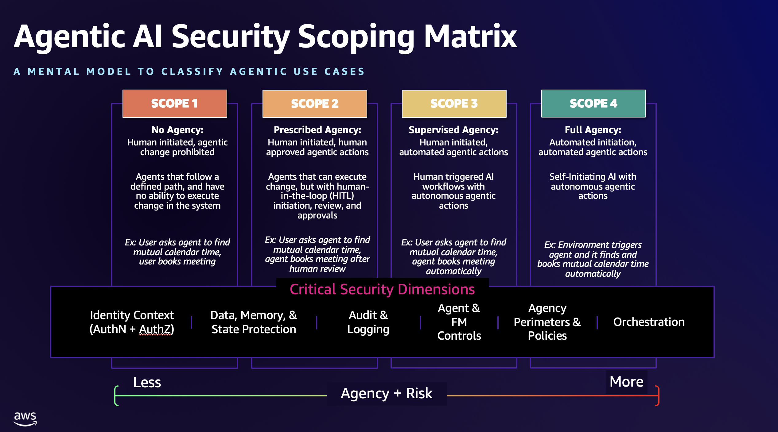
Working with customers and the community, we’ve identified four architectural scopes that represent the evolution of agentic AI systems based on two critical dimensions: level of human oversight compared with autonomy and the level of agency the AI system is permitted to act within. Each scope introduces new capabilities—and corresponding security requirements—that organizations must prioritize when addressing agentic AI risk. Figure 1 shows the Agentic AI Security Scoping Matrix.

Figure 1 – The Agentic AI Security Scoping Matrix

In this most basic scope, systems operate with human-initiated processes and no autonomous or even human-approved change capabilities through the agent itself. The agents are, essentially, read-only. These systems follow predefined execution paths and operate under strict human-triggered workflows, which are usually predefined and follow discrete steps, but could be augmented with non-deterministic outputs from an FM. Security focuses primarily on process integrity and boundary enforcement, helping operations remain within predetermined limits and agents are highly controlled and prohibited from change execution and unbounded actions.

Key characteristics:

• Agents can’t directly execute change in the environment
• Fixed step-by-step execution following predetermined paths
• Generative AI components process data within individual workflow nodes
• Conditional branching only where explicitly designed into the workflow
• No dynamic planning or autonomous goal-seeking behavior
• State persistence limited to workflow execution context
• Tool access restricted to specific predefined workflow steps

Security focus: Protecting data integrity within the environment and restricting agents to not exceed their boundaries, especially limits around environment and data modification. Primary concerns include securing state transitions between steps, validating data passed between workflow nodes, and preventing AI components from modifying the orchestration logic or escaping their designated boundaries within the workflow.

Example: We will use a very simplistic example, across all four scopes, of a use case for an agent that is designed to help you create calendar invites. Let’s say you need to book a meeting with another colleague. In Scope 1, you might have an agent that you instantiate through a workflow or prompt to look at your calendar and your colleague’s calendar for available meeting times. In this case, you initiate the request, and the agent executes a contextual search using a Model Context Protocol (MCP) server connected to your enterprise calendaring application. The agent is only allowed to look at available times, analyze the best times to meet, and provide a response back, which a human can then use to manually set up a meeting. In this example, the human defines specific workflows and orchestrations (no agency) and reviews and approves the actions taken (no autonomous change).

Moving up in agency and risk, Scope 2 systems also are instantiated by a human, but now have the potential to perform actions—limited agency—that could change the environment. However, all actions taken by an agent require explicit human approval for all actions of consequence—commonly referred to as human in the loop or HITL. These systems can gather information, analyze data, and prepare recommendations, but cannot execute actions that modify external systems or access sensitive resources without human authorization. Agents can also request human input to clarify ambiguities, provide missing context, or optimize their approach before presenting recommendations.

Key characteristics:

• Agents can execute change in the environment with human review and approval
• Real-time human oversight with approval workflows
• Bidirectional human interaction—agents can query humans for context
• Limited autonomous actions restricted to read-only operations (such as, querying data, running analysis jobs, and so on)
• Agent-initiated requests for clarification or additional information
• Audit trails of all human approval decisions and context exchanges

Security focus: Implementing robust approval workflows and preventing agents from bypassing human authorization controls. Key concerns include preventing privilege escalation, enforcing appropriate identity contexts, securing the approval process itself, validating human-provided context to prevent injection attacks, and maintaining visibility into all agent recommendations and their rationale.

Example: In our calendaring example, a Scope 2 agentic system is instantiated by a human. The agent then looks up the stakeholders’ calendar availability, does its analysis, returns a recommendation for a meeting time to the user, and asks the user if they want the agent to send the invitation out on their behalf. The user looks at the response and recommendation of the agent, validates that it meets their requirements, and then acknowledges and approves the agent’s request to modify the calendars and send the invitation. In this example, the human orchestrates a structured workflow, but the agent now can instantiate human reviewed change through bounded actions (limited agency and limited autonomy).

In Scope 3, we expand the agency to allow for a greater sense of agentic autonomy—high agency—in execution. These are AI systems that execute complex autonomous tasks that are initiated by humans (or at least from an upstream human-managed workflow), with the ability to make decisions and take actions to connected systems without further approval or HITL mechanisms. Humans define the objectives and trigger execution, but agents operate independently to achieve goals through dynamic planning and tool usage. During execution, agents can request human guidance to optimize trajectory or handle edge cases, though they can continue operating without it.

Key characteristics:

• Agents can execute change in the environment, with no (or optional) human interaction or review
• Human-triggered execution with autonomous task completion
• Dynamic planning and decision-making during execution
• Optional human intervention points for trajectory optimization
• Human ability to adjust parameters or provide context mid-execution
• Direct access to external APIs and systems for task completion
• Persistent memory across extended execution sessions
• Autonomous tool selection and orchestration within defined boundaries

Security focus: Implementing comprehensive monitoring of agent actions during autonomous execution phases and establishing clear agency boundaries for agent operations—the bounds you’re willing to let the agents operate within, and actions that would be out of bounds and must be prevented. Critical concerns include securing the human intervention channel to prevent unauthorized modifications, preventing scope creep during task execution, implementing trusted identity propagation constructs, monitoring for behavioral anomalies, and validating that agents remain aligned with original human intent throughout extended operations even when trajectory adjustments are made.

Example: In our calendaring example, a Scope 3 agentic system can still be instantiated by a human. The agent then looks up the stakeholders’ calendar availability, does its analysis, and returns a recommendation for a meeting time to the user; however, it’s within the agent’s bounds to act upon its own recommendation on behalf of the user to automatically book the best available slot. The user is not prompted or expected to give the agent permission to do so prior to its actions. The result is that all stakeholders have a calendar entry added to their calendar in the context of the calling human user. In this example, the human defines an outcome but with more freedom for the agent to determine how to achieve that goal, and the agent now can take autonomous action without human review (high agency and high autonomy).

Scope 4 includes fully autonomous AI systems that can initiate their own activities based on environmental monitoring, learned patterns, or predefined conditions, and execute complex tasks without human intervention. These systems represent the highest level of AI agency, operating continuously and making independent decisions about when and how to act. It’s key to note that AI systems within Scope 4 could have full agency when executing within their designed bounds; therefore, it’s critical that humans maintain supervisory oversight with the ability to provide strategic guidance, course corrections, or interventions when needed. Continuous compliance, auditing, and full-lifecycle management mechanisms, both human and automated reviews, which could also be aided by AI, are critical to successfully securing and governing Scope 4 agentic AI systems while limiting risk.

Key characteristics:

• Self-directed activity initiation based on environmental triggers
• Continuous operation with minimal human oversight or HITL processes during execution
• Human ability to inject strategic guidance without disrupting operations
• High to full degrees of autonomy in goal setting, planning, and execution
• Dynamic interaction with multiple external systems and agents
• Capability for recursive self-improvement and capability expansion

Security focus: Implementing advanced guardrails for behavioral monitoring, anomaly detection, scope-based tool access controls, and fail-safe mechanisms to prevent runaway operations. Primary concerns include maintaining alignment with organizational objectives, securing human intervention channels against adversarial manipulation, preventing unauthorized capability expansion, preventing human oversight mechanisms from being disabled by the agent, and enabling graceful degradation when agents encounter unexpected situations.

Example: Let’s look at how we might deploy our AI calendaring example in Scope 4. Let’s say you have implemented a generative AI meeting summarizer. This agent is automatically enabled when you host a web conference. At the conclusion of the meeting, the calendaring agent sees a new meeting occurred from the meeting summarizer agent. It looks at the action items that were summarized and determines that six people agreed to a whiteboard session on Friday. The calendaring agent might either have a statically defined API configuration or leverage dynamic discovery on MCP servers to help with calendaring. It then finds availability for the six identified resources and books the best available slot. It then uses the appropriate identity context of the user who is asking for the meeting to book the meeting autonomously. At no point does a user directly instantiate the request for calendaring; it is fully automated and driven off environment changes that the agent is instructed to look for (full agency and full autonomy).

In the context of the security scoping matrix, let’s compare how autonomy and agency characteristics shift depending on the scope:

Table 1 – Scope impacts on agency and autonomy levels

Each architectural scope requires specific security controls and considerations across six critical dimensions. Table 2 illustrates how security requirements escalate with increasing agency and autonomy:

Table 2 — Critical security dimensions per scope

Now that we’ve outlined each of the scopes and the associated levels of agency and autonomy, let’s discuss some primary security challenges per scope and key considerations that should be taken to address the associated risks.

Scope 1: No agency
Primary security challenges: Protecting workflow integrity, preventing prompt injection from breaking predetermined flows, and maintaining isolation between workflow executions.

Implementation considerations:

• Comprehensive monitoring with anomaly detection
• Strict data validation and integrity checking
• Input validation at each workflow step boundary
• Immutable workflow definitions with version control
• State encryption and validation between workflow nodes
• Monitoring for attempts to escape workflow boundaries
• Segregation between different workflow executions
• Fixed timeout and resource limits per workflow step
• Audit trails showing actual compared to expected execution paths

Scope 2: Prescribed agency
Primary security challenges: Securing approval workflows, preventing human authorization bypass, and maintaining oversight effectiveness.

Implementation considerations:

• Multi-factor authentication for all human approvers
• Cryptographically signed approval decisions
• Securing bidirectional human-agent communication channels
• Time-bounded approval tokens with automatic expiration
• Comprehensive logging of all approval interactions
• Regular training for human approvers on agent capabilities and risks

Scope 3: Supervised agency
Primary security challenges: Maintaining control during autonomous execution, scope management, explainability and auditability, and behavioral monitoring.

Implementation considerations:

• Clear execution boundaries defined at initiation
• Real-time monitoring of agent actions during execution
• Automated kill switches for runaway processes
• Non-blocking intervention mechanisms
• Behavioral baselines for normal agent operations
• Regular validation of agent alignment with original objectives

Scope 4: Full agency
Primary security challenges: Continuous behavioral validation, enforcing agency boundaries, preventing capability drift, and maintaining organizational alignment.

Implementation considerations:

• Advanced AI safety techniques including reward modeling
• Continuous monitoring with machine learning-based anomaly detection
• Automated response systems for behavioral deviations
• Regular alignment validation through systematic testing
• Tamper-proof human override mechanisms
• Failsafe mechanisms that can halt operations when confidence drops

Successful agentic deployments share common patterns that balance autonomy with control.

Progressive autonomy deployment: Start with Scope 1 or 2 implementations and gradually advance through the scopes as organizational confidence and security capabilities mature. This approach minimizes risk while building operational experience. Be cautious and selective when analyzing use cases and bounding controls for Scope 4 implementations and review your ability to address risks at the lower scopes and how risks increase as you move further up the levels.

Layered security architecture: Implement defense-in-depth with security controls at multiple levels—network, application, agent, and data layers—to safeguard that compromise at one level doesn’t lead to complete system failure. Although the combination of these controls is what enables a high security bar, be sure to spend considerable efforts on making sure that identity and authorization concerns are addressed—for both machines and humans. This helps prevent issues such as the confused deputy problem—when a human or service with lesser permissions is able to elevate permissions through agents that might themselves have more entitlements and privileges.

Continuous validation loops: Establish automated systems that continuously verify agent behavior against expected patterns, and that have escalation procedures for when deviations are detected. Auditability and explainability are key requirements to confirm that agents are performing within the bounds intended and to help you determine control effectiveness, adjust parameters, and validate your orchestration workflows.

Human oversight integration: Even in highly autonomous systems, maintain meaningful human oversight through strategic checkpoints, behavioral reporting, and manual override capabilities. It might be reasonable to assume that human oversight reduces when moving from Scope 1 to Scope 4 agency, but the truth is that it simply shifts focus. For example, the human requirement to instantiate, review, and approve certain agentic actions is higher in Scopes 1 and 2 and lower in Scopes 3 and 4; however, the human requirement to audit, assess, validate, and implement more complex security and operational controls is much higher in Scopes 4 and 3 than they are in Scopes 2 and 1.

Graceful degradation: Design systems to automatically reduce autonomy levels when security events are detected, allowing operations to continue safely while human operators investigate. If your agents start to act in ways that go beyond the intended bounds of their design, anomalous behavior is detected, or they begin to perform actions deemed particularly risky or sensitive to your business, then consider having detective controls that will automatically inject tighter restrictions such as requiring more HITL or reducing the actions an agent can take. You might do this as incremental degradation or, you might choose to disable the agent if it’s acting in ways that negatively impact the environment. These agentic safety mechanisms that can implement additional restrictions or even disable an agent should be considered when building or deploying agents.

The Agentic AI Security Scoping Matrix provides a structured mental model and framework for understanding and addressing the security challenges of autonomous agentic AI systems across four distinct scopes. By accurately assessing your current scope and implementing appropriate controls across all six security dimensions, organizations can confidently deploy agentic AI while managing the landscape of associated risks.

The progression from basic and highly constrained agents to fully autonomous and even self-directing agents represents a fundamental shift in how we approach AI security. Each scope requires specific security capabilities, and organizations must build these capabilities systematically to support their agentic ambitions safely.

To implement the Agentic AI Security Scoping Matrix in your organization:

1. Assess your current agentic use cases and maturity against the four scopes to understand your security requirements and associated risks. Integrate it into your procurement and SDLC processes.
2. Identify capability gaps across the six security dimensions for your target scope.
3. Develop a progressive deployment strategy that builds security capabilities as you advance through scopes.
4. Implement continuous monitoring and behavioral analysis appropriate for your scope level.
5. Establish governance processes for scope progression and security validation.
6. Train your teams on the unique security challenges of each scope.

You can find additional information on the Agentic AI Security Scoping matrix here, along with additional information on AI security topics. For additional resources on securing AI workloads, see the AI for security and security for AI: Navigating Opportunities and Challenges whitepaper and explore purpose-built platforms designed for the unique challenges of agentic AI.