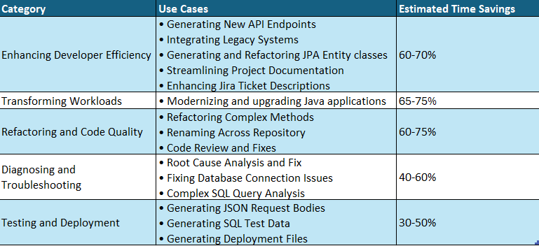
This post was co-authored by Mike Araujo Principal Engineer at Medidata Solutions.
The life sciences industry is transitioning from fragmented, standalone tools towards integrated, platform-based solutions. Medidata, a Dassault Systèmes company, is building a next-generation data platform that addresses the complex challenges of modern clinical research. In this post, we show you how Medidata created a unified, scalable, real-time data platform that serves thousands of clinical trials worldwide with AWS services, Apache Iceberg, and a modern lakehouse architecture.
Challenges with legacy architecture
As the Medidata clinical data repository expanded, the team recognized the shortcomings of the legacy data solution to provide quality data products to their customers across their growing portfolio of data offerings. Several data tenants began to erode. The following diagram shows Medidata’s legacy extract, transform, and load (ETL) architecture.
Built upon a series of scheduled batch jobs, the legacy system proved ill-equipped to provide a unified view of the data across the entire ecosystem. Batch jobs ran at different intervals, often requiring a sufficient degree of scheduling buffer to make sure upstream jobs completed within the expected window. As the data volume expanded, the jobs and their schedules continued to inflate, introducing a latency window between ingestion and processing for dependent consumers. Different consumers operating from various underlying data services further magnified the problem as pipelines had to be continuously built across a variety of data delivery stacks.
The expanding portfolio of pipelines began to overwhelm existing maintenance operations. With more operations, the opportunity for failure expanded and recovery efforts further complicated. Existing observability systems were inundated with operational data, and identifying the root cause of data quality issues became a multi-day endeavor. Increases in the data volume required scaling considerations across the entire data estate.
Additionally, the proliferation of data pipelines and copies of the data in different technologies and storage systems necessitated expanding access controls with enhanced security features to make sure only the correct users had access to the subset of data to which they were permitted. Making sure access control changes were correctly propagated across all systems added a further layer of complexity to consumers and producers.
Solution overview
With the advent of Clinical Data Studio (Medidata’s unified data management and analytics solution for clinical trials) and Data Connect (Medidata’s data solution for acquiring, transforming, and exchanging electronic health record (EHR) data across healthcare organizations), Medidata introduced a new world of data discovery, analysis, and integration to the life sciences industry powered by open source technologies and hosted on AWS. The following diagram illustrates the solution architecture.
Fragmented batch ETL jobs were replaced by real-time Apache Flink streaming pipelines, an open source, distributed engine for stateful processing, and powered by Amazon Elastic Kubernetes Service (Amazon EKS), a fully managed Kubernetes service. The Flink jobs write to Apache Kafka running in Amazon Managed Apache Kafka (Amazon MSK), a streaming data service that manages Kafka infrastructure and operations, before landing in Iceberg tables backed by the AWS Glue Data Catalog, a centralized metadata repository for data assets. From this collection of Iceberg tables, a central, single source of data is now accessible from a variety of consumers without additional downstream processing, alleviating the need for custom pipelines to satisfy the requirements of downstream consumers. Through these fundamental architectural changes, the team at Medidata solved the issues presented by the legacy solution.
Data availability and consistency
With the introduction of the Flink jobs and Iceberg tables, the team was able to deliver a consistent view of their data across the Medidata data experience. Pipeline latency was reduced from days to minutes, helping Medidata customers realize a 99% performance gain from the data ingestion to the data analytics layers. Due to Iceberg’s interoperability, Medidata users saw the same view of the data regardless of where they viewed that data, minimizing the need for consumer-driven custom pipelines because Iceberg could plug into existing consumers.
Maintenance and durability
Iceberg’s interoperability provided a single copy of the data to satisfy their use cases, so the Medidata team could focus its observation and maintenance efforts on a five-times smaller subset of operations than previously required. Observability was enhanced by tapping into the various metadata components and metrics exposed by Iceberg and the Data Catalog. Quality management transformed from cross-system traces and queries to a single analysis of unified pipelines, with an added benefit of point in time data queries thanks to the Iceberg snapshot feature. Data volume increases are handled with out-of-box scaling supported by the entire infrastructure stack and AWS Glue Iceberg optimization features that include compaction, snapshot retention, and orphan file deletion, which provide a set-and-forget experience for solving a number of common Iceberg frustrations, such as the small file problem, orphan file retention, and query performance.
Security
With Iceberg at the center of its solution architecture, the Medidata team no longer had to spend the time building custom access control layers with enhanced security features at each data integration point. Iceberg on AWS centralizes the authorization layer using familiar systems such as AWS Identity and Access Management (IAM), providing a single and durable control for data access. The data also stays entirely within the Medidata virtual private cloud (VPC), further reducing the opportunity for unintended disclosures.
Conclusion
In this post, we demonstrated how legacy universe of consumer-driven custom ETL pipelines can be replaced with a scalable, high-performant streaming lakehouses. By putting Iceberg on AWS at the center of data operations, you can have a single source of data for your consumers.
As data volumes continue to grow exponentially, there is increasing pressure to optimize search infrastructure costs while maintaining the high performance and reliability that mission-critical workloads demand. Many companies find themselves managing complex, expensive search systems that require significant operational overhead and limit their ability to scale efficiently. The challenge becomes even more acute when organizations need to migrate between search systems, a process that traditionally involves substantial downtime, complex data synchronization, and significant impact on business operations. Enterprise applications cannot afford service interruptions that could impact customer experiences, business intelligence, or operational continuity. Migration strategies need to deliver cost optimization and operational improvements while maintaining zero downtime and facilitating complete data integrity throughout the transition process.
Founded in 2013, Octus, formerly Reorg, is the essential credit intelligence and data provider for the world’s leading buy side firms, investment banks, law firms and advisory firms. By surrounding unparalleled human expertise with proven technology, data and AI tools, Octus unlocks powerful truths that fuel decisive action across financial industries.
This post highlights how Octus migrated its Elasticsearch workloads running on Elastic Cloud to Amazon OpenSearch Service. The journey traces Octus’s shift from managing multiple systems to adopting a cost-efficient solution powered by OpenSearch Service. Along the way, we share the architecture choices and implementation strategies that made the migration successful. The result is uninterrupted service availability throughout migration, with improved performance and greater cost efficiency.
Strategic requirements
We identified several requirements that made Amazon OpenSearch Service the right choice for their migration:
Cost efficiency: The OpenSearch Service pricing model enabled us to optimize cloud spend without compromising performance.
Responsive support: AWS provided dependable, high-quality support to accelerate issue resolution and instill confidence.
Consistent reliability: OpenSearch Service provides an SLA up to 99.99% offering the reliability required for Octus’s mission-critical workloads.
Seamless migration with no query downtime: Migration Assistant for Amazon OpenSearch Service provided Octus with a migration path while maintaining uninterrupted query availability during the migration, facilitating business continuity.
Operational simplification: Consolidating onto AWS reduced infrastructure complexity while maintaining high security standards.
Solution overview
The Migration Assistant for Amazon OpenSearch Service provides a suite of tools to aid in Elasticsearch to OpenSearch Service migrations. Octus use the following capabilities for their migration:
Metadata migration: The tool enabled Octus to migrate dozens of indices with diverse mappings and settings. When a backward incompatibility was identified with timestamp metadata, a custom JavaScript transformation, integrated directly into the Migration Assistant tooling, was applied to automatically adjust the mappings across the indices and facilitate compatibility.
Historical data migration: Octus used Reindex-from-Snapshot to migrate the historical documents from a point-in-time snapshot of the source cluster, scaling this process without impacting the source cluster since the snapshot was stored in Amazon Simple Storage Service (Amazon S3). Reindex-from-Snapshot also enabled Octus to adjust the sharding scheme during migration, helping to optimize cluster performance on the target.
Live Traffic Replay: Once backfill was complete, Octus used Migration Assistant’s Traffic Replayer to send the captured live traffic (from the Traffic Capture Proxy) to the target cluster with required request transformations for OpenSearch Service compatibility, resulting in the target cluster containing the documents from the source cluster with updates being performed in real time.
The following diagram illustrates the implementation architecture diagram for this migration.
Figure 1 – Migration Assistant architecture with migration steps
For more information about the Migration Assistant for Amazon OpenSearch Service, visit the AWS Solutions home page.
Each node in the diagram correlates to the following steps in the migration process:
Client traffic is directed to the existing cluster.
Using the migration console, a point-in-time snapshot is taken. Once the snapshot completes, the Metadata Migration Tool is used to establish indexes, templates, component templates, and aliases on the target cluster. With continuous traffic capture in place, Reindex-from-Snapshot, migrates data from the source.
Once Reindex-from-Snapshot is complete, captured traffic is replayed from Amazon Managed Streaming for Apache Kafka (Amazon MSK) to the target cluster by Traffic Replayer.
Performance and behavior of traffic sent to the source and target clusters are compared by reviewing logs and metrics.
After confirming that the target cluster’s functionality meets expectations, clients are redirected to the new target.
Complete migration and optimization journey
Octus’s migration from Elastic Cloud to Amazon OpenSearch Service encompassed both the core migration effort and subsequent optimization phases. The goal was to successfully migrate the search infrastructure, applications, and data from Elastic Cloud to a new OpenSearch Service domain with minimal disruption, while continuously optimizing performance and costs based on real-world usage data.
Octus used their in-house custom infrastructure frameworks (their internal tooling for infrastructure automation) to build, deploy and monitor the target OpenSearch Service 1.3 domain, establishing a solid foundation for the migration. This approach used familiar internal processes while moving to the fully managed AWS service. Refer to AWS documentation to implement security best practices when using OpenSearch Service.
Pre-migration optimization
Prior to initiating the migration, Octus conducted optimization activities on the source Elasticsearch cluster to streamline the migration process. This included removing unused indexes that had accumulated over time and removing large documents that would unnecessarily extend migration duration and increase storage transfer costs. These preparatory steps significantly reduced the data volume requiring migration and minimized the overall migration complexity, enabling more efficient use of the Migration Assistant tools.
Technical constraints and version considerations
The migration involved specific version compatibility challenges that influenced the technical approach. The source Elasticsearch cluster was running version 7.17, and the Python client applications were also constrained to Elasticsearch 7.17 compatibility. To support the transition, the team used Reindex-from-Snapshot, which enables cross-system migrations by reindexing data from existing snapshots into a new OpenSearch Service cluster. RFS also rewrites indices created on older versions of Lucene, simplifying future upgrades to the latest version of OpenSearch Service. While evaluating a move to OpenSearch 1 or 2, Octus selected OpenSearch 1.3 as the target to minimize client-side changes and reduce migration complexity, while positioning themselves for simpler upgrades later.
The version selection particularly impacted the R application environment, as R language (an open-source programming language for statistical computing and data analysis) lacked native OpenSearch 1.3 client support. This constraint required Octus to develop a custom client solution using the ropensci/elastic library to integrate with the new OpenSearch Service domain. The Python environment presented similar challenges, where the Elasticsearch 7.17 client constraints necessitated careful consideration of the migration approach. These client compatibility concerns were among the factors that influenced the choice of Migration Assistant tools over traditional snapshot-based methods, as the Migration Assistant provided better support for managing version-specific client interactions during the transition.
Looking forward, Octus plans to upgrade to newer OpenSearch versions as their application stack evolves and client library support matures, so that they can leverage the latest features and performance improvements while maintaining the stability achieved through this migration.
Application modernization across multiple languages
The application changes represented a significant technical undertaking across multiple programming environments:
Legacy PHP systems (5.6 and Laravel 4.2): Octus handled mapping type deprecation on OpenSearch requests as specifying these mapping types are not supported, while continuing to use the elasticsearch connector library with username/password authentication.
Modern PHP applications (8.1 and Laravel 9): These underwent more comprehensive changes, replacing the elasticsearch/elasticsearch library with the opensearch-project/opensearch-php client and leveraging IAM authentication to connect to the clusters.
Python environment: Applications spanning versions 3.8, 3.10, 3.11, and 3.13 with Django frameworks 2.1, 3.2, and 5.2 required replacing the elasticsearch library with opensearch-py and transitioning to IAM authentication.
R applications: For R 4.5.1 applications, Octus utilized a custom library ropensci/elastic to facilitate compatibility.
Traffic routing and enhanced monitoring
To facilitate the migration, Octus redirected their existing clients to route requests to the source cluster through Migration Assistant’s Traffic Capture Proxy, migrating the data from live traffic to their target cluster.
The monitoring infrastructure underwent significant enhancement during this process. Octus’s observability infrastructure monitors the overall health of OpenSearch Service clusters which includes cluster manager and data nodes, network, data storage, security and IAM access. It also monitors the indexing and search performance of their applications. This alleviated the need for a separate monitoring cluster as logs and metrics were shipped directly to Datadog, significantly improving observability. The Datadog monitors were defined using Infrastructure-as-Code and integrated seamlessly into their infrastructure frameworks.
Cutover and initial results
The Site Reliability Engineering team meticulously planned the release, achieving a successful migration from Elasticsearch to OpenSearch Service and cutover of the Elasticsearch client to the OpenSearch Service clients with no downtime for the system application and zero data loss. The initial migration phase resulted in a 52% cost reduction while achieving operational benefits including zero downtime for the system app, no data loss, full Infrastructure-as-Code implementation for infrastructure and monitoring, and enhanced observability.
Post-migration optimization
Following the migration, Octus conducted comprehensive optimization based on operational data from production and other environments in the new OpenSearch Service setup. This real-world usage data provided valuable insights into actual resource consumption, enabling informed decisions regarding further cluster resizing.
Through usage metric analysis and strategic resizing, Octus aligned cluster size more precisely with operational needs, facilitating continued performance while minimizing expenditure. This optimization phase delivered an additional 33% cost reduction compared to the original Elastic Cloud costs, bringing the total reduction to 85% while maintaining consistent and optimal performance.
Operational monitoring
Octus uses Datadog to monitor both search and indexing latency providing real-time visibility into Amazon OpenSearch Service cluster performance. The following screenshot showcases how custom Datadog dashboards provide a live view of the OpenSearch Service clusters. This visualization offers both a high-level overview and detailed insights into the ingestion process, helping us understand the storage and document count. The bottom half of the dashboard presents a time-series view of individual node health and performance metrics like read and write latency, throughput and IOPS.
Figure 2 – DataDog dashboards
Migration observability
Migration Assistant for Amazon OpenSearch Service provides several dashboards to observe and validate the progress of a migration. By using these observability features customers can track both backfill and live capture and replay progress, facilitating confidence before switching production workloads to the target cluster.The following graphs are an example from Octus’s migration, where approximately 4TB of data was migrated in about 9 hours (from 08:00 to 17:00).
Figure 3 – Backfill progress by disk usage
Figure 4 – Backfill progress by searchable documents
Once the backfill is complete, the captured traffic is replayed to synchronize ongoing activity between the source and target clusters.
At the time the backfill finished (around 17:00), the target cluster was approximately 467 minutes behind the source. The replay process rapidly reduced this lag by processing captured traffic at a faster rate than it was originally ingested at the source.
Figure 5 – Replay lag after backfill completion
When the lag time reached 0, the target cluster was fully in sync and production traffic could safely be rerouted. Octus chose to observe replayed traffic on the target for several days before making the final switchover.
Achieving excellence
Octus’s migration to Amazon OpenSearch Service has yielded remarkable results:
Scalability – Octus has almost doubled the number of documents available for Q&A across three environments in days instead of weeks. Their use of Amazon Elastic Container Service (Amazon ECS) with AWS Fargate with auto scaling rules and controls gives them elastic scalability for their services during peak usage hours.
Cost reduction – By moving away from Elastic Cloud to OpenSearch Service, Octus’s monthly infrastructure costs are now 85% lower.
Enhanced search performance – Octus maintained consistent response times throughout the migration with no negative impact on latency, while achieving a 20% improvement in query throughput and overall search performance.
Zero downtime – Octus experienced zero downtime during migration and 100% uptime overall for the whole application.
Reduced operational overhead – Post-migration, Octus’s DevOps and SRE teams see 30% less maintenance burden and overheads. Supporting SOC2 compliance is also straightforward now that they’re using one system.
Accelerated timeline delivery – The entire migration was completed ahead of schedule, moving from planning to full completion in under one quarter.
“Moving from Elastic Cloud to Amazon OpenSearch Service was a key component of our broader strategy to minimize third-party dependencies and strengthen the reliability of Octus’ system infrastructure. Migration Assistant for Amazon OpenSearch Service enabled us to execute a seamless transition with zero data loss and virtually no downtime for our users.” – Vishal Saxena, CTO, Octus
Conclusion
In this post, we showed you how Octus successfully migrated their Elasticsearch workloads from Elastic Cloud to Amazon OpenSearch Service using the Migration Assistant for OpenSearch Service, achieving zero downtime and significant operational improvements.
The Migration Assistant for OpenSearch Service supported this complex migration through its comprehensive suite of tools. The Metadata Migration capability migrated dozens of indices with diverse mappings and settings, with custom JavaScript transformations handling backward incompatibilities. Reindex-from-Snapshot migrated the historical documents from point-in-time snapshots without impacting the source cluster, while also optimizing the sharding scheme for improved performance. Live Traffic Replay made sure the target cluster remained synchronized with real-time updates throughout the migration process.
The migration delivered substantial results across the dimensions. Octus achieved an 85% reduction in monthly infrastructure costs while nearly doubling the number of documents available for search across three environments. Search performance improved by 20% in query throughput with consistent response times and no negative impact on latency. The migration maintained zero downtime and 100% uptime for the entire application, with DevOps and SRE teams experiencing 30% less maintenance burden and operational overhead. The entire migration was completed ahead of schedule in under one quarter.
To learn more about the Migration Assistant for OpenSearch Service and how it can help you achieve similar results, visit the AWS Solutions home page.
Visit Octus to learn how we deliver rigorously verified intelligence at speed and create a complete picture for professionals across the entire credit lifecycle. Follow Octus on LinkedIn and X.
If you’ve developed AWS CloudFormation templates, you know the drill; write YAML(YAML Ain’t Markup Language) in your IDE(Integrated Development Environment), switch to the AWS Management Console to validate, jump to documentation to verify property names. Then run CFN Lint(Cloudformation Linter) in your terminal, deploy and wait, then troubleshoot failures back in the console. This constant context switching between your IDE, AWS Console, documentation pages, and validation tools fragments your workflow and kills productivity. What should take 30 minutes often stretches into hours of iteration cycles.
Today, we’re excited to introduce the CloudFormation IDE Experience, a comprehensive solution that brings the entire CloudFormation development lifecycle into your IDE. No more context switching. No more fragmented workflows. Just one unified, intelligent development experience from authoring to deployment.
In this post, you’ll learn how the Cloudformation IDE Experience transforms your workflow with intelligent authoring, real-time validation, AWS integration, and more.
What is the CloudFormation IDE Experience?
The CloudFormation IDE Experience reimagines how you build infrastructure as code by creating an end-to-end development loop entirely within your IDE. Unlike generic YAML or JSON editors, this is a CloudFormation-first solution built specifically for infrastructure developers.
This solution covers the complete lifecycle; from intelligent authoring with smart code completion and navigation that understands CloudFormation semantics, to real-time multi-layer validation that catches issues before deployment. It provides direct AWS integration for seamless resource imports and stack visibility, monitors configuration drift between your templates and deployed resources, and includes server-side pre-deployment checks that prevent common deployment failures. The result? A development environment that understands your infrastructure code as deeply as your IDE understands your application code.
Core Features
Quick Project Setup with CFN Init
CFN Init streamlines project setup by creating a structured CloudFormation project with environment configurations in seconds. Run “CFN Init: Initialize Project” from the Command Palette, configure your environments (dev, staging, production), and associate each with an AWS profile.
The CloudFormation Explorer displays your environments, letting you switch between them with a single click. Each environment maintains its own deployment settings and parameter values, eliminating manual configuration and ensuring consistent deployments across your infrastructure lifecycle.
Intelligent Authoring with Intelligent Code Completion
The IDE understands CloudFormation semantics and provides context-aware suggestions as you type. Only required properties appear automatically, while optional properties surface on hover, so when you add a Properties section to an EC2 VPC resource, nothing appears because it has no required properties. Create a subnet, however, and VpcId appears immediately because it’s required.
When you use !GetAtt or !Ref, the IDE knows exactly which attributes and resources are available. Navigation features like go-to-definition for logical IDs and hover tooltips let you explore complex templates without losing context. The IDE also provides full support for CloudFormation intrinsic functions and pseudo parameters.
Multi-Layer Validation System
The IDE provides comprehensive validation at multiple levels:
Static Validation (Real-time)
CloudFormation Guard Integration: Security and compliance checks using AWS Security pillar rules. For example, it automatically flags insecure configurations like MapPublicIpOnLaunch: true on subnets
CFN Lint Integration: Advanced syntax and logic validation, including overlapping CIDR block detection, resource dependency validation, and property checks beyond basic schema validation
Interactive Error Resolution When errors occur, the IDE doesn’t just highlight them, it helps you fix them. Contextual error messages explain what’s wrong and why it matters, while one-click quick fixes automatically correct common issues like missing required properties or invalid reference formats. If you reference a non-existent resource, the IDE suggests valid alternatives from your template. Reference an invalid attribute with !GetAtt, the IDE immediately shows which attributes are actually available for that resource type.
AWS Resource Integration (CCAPI)
Import existing AWS resources directly into your templates using the Cloud Control API (CCAPI). Browse live resources and view all CloudFormation stacks in your AWS account from within the IDE. Pull resource configurations directly into your template with one click, complete with accurate property values. This transforms existing infrastructure into Infrastructure-as-Code without manual reconstruction or switching to the console to look up property values.
Server-Side Validation
Before you deploy, the IDE performs comprehensive server-side validation through AWS’s intelligent validation service that analyzes your CloudFormation templates against real-world deployment patterns and catches issues static analysis can’t detect.
The AWS’s intelligent validation service uses AWS-managed hooks to analyze your change sets before execution across three categories. Enhanced template validation covers CFN Lint blind spots like transforms and parameter values. Primary identifier conflict detection finds existing resources with the same identifiers before you attempt deployment. Resource state validation checks resource readiness ensuring, for example, that Amazon Simple Storage Service(S3) buckets are empty before deletion attempts.
This validation is based on analysis of the top CloudFormation failure patterns, helping you catch issues before they cause rollbacks or failed states.
Getting Started
Getting started with the CloudFormation IDE Experience is straightforward:
Prerequisite:
Install an IDE that supports the CloudFormation extension, such as Visual Studio Code, Kiro
Download the CloudFormation extension for your platform (available through the AWS Toolkit)
No complex dependency management or schema updates required—all configuration and updates are handled automatically.
Let’s See How It Works
Let’s walk through a practical example that demonstrates the IDE experience in action. We’ll build a simple Amazon Virtual Private Cloud (Amazon VPC) infrastructure with subnets and an S3 bucket.
Setting Up Your Project
Start by initializing a new CloudFormation project. Open the Command Palette, run “CFN Init: Initialize Project”, choose your project location, and set up environments. For this example, create a “beta” environment and associate it with your AWS development profile. The IDE creates your project structure with configuration files ready to use. You can now select your “beta” environment from the CloudFormation Explorer to ensure all deployments use the correct settings.
Figure 1: Initializing a CloudFormation project with environment configuration
Starting with Intelligent Authoring
Create a new CloudFormation template and start typing AWS::EC2::VPC. The IDE provides intelligent completions as you type.
Figure 2.0: Resource type auto-completion with CloudFormation-aware IntelliSense
When you add the Properties section, notice something interesting: nothing appears automatically. That’s because Amazon Elastic Compute Cloud (Amazon EC2) VPC has no required properties.
Figure 2.1: No automatic suggestions for VPC properties since none are required
Hover over Properties to see all available options with their types and documentation links.
Figure 2.2: Hover information displaying optional properties and their documentation
Add a CIDR block, then create a subnet. This time, when you type Properties, VpcId appears immediately because it’s required.
Figure 2.3: Required properties VpcID automatically suggested for EC2 Subnet
The IDE provides the resource names in your template, and when you use !GetAtt or !Ref, it knows which attributes are available for each resource type.
Figure 2.4: Type-aware completions for intrinsic functions like !GetAtt & !Ref
Real-Time Validation in Action
As you continue building, add MapPublicIpOnLaunch: true to make a public subnet. Immediately, a blue squiggly line appears.
Figure 3: CloudFormation Guard warning highlighted in real-time
Hovering reveals a CloudFormation Guard warning from the AWS Security pillar rules: this configuration isn’t recommended for security compliance.
Figure 3.1: Security compliance warning with detailed explanation
Create a second subnet by copying the first, but now red squiggly lines appear. CFN Lint has detected overlapping CIDR blocks between your two subnets – an issue that would fail during deployment. You can fix it immediately with the contextual information provided.
Figure 3.2: CFN Lint error detection for overlapping CIDR blocks providing detailed error information helping you resolve the issue quickly
Importing Existing Resources
Now you need an S3 bucket. Instead of writing it from scratch, open the Resource Explorer panel on the left. Using CCAPI integration, you can see all your existing AWS resources. Select an S3 bucket and click “Import resource state”. The IDE pulls in the complete resource configuration with all properties already set. You can now iterate on this resource without needing to remember or look up all the configuration details.
Figure 4: Automatically imported resource configuration from live AWS resources
Developer Experience Benefits
The CloudFormation IDE Experience delivers measurable improvements across productivity and quality:
Productivity Gains:
Reduced context switching: Keep your entire workflow in one place
Faster iteration cycles: Catch and fix issues in seconds, not minutes or hours
Shift-left validation: Identify problems before deployment, not after
Intelligent assistance: Spend less time in documentation, more time building
Quality Improvements:
Proactive error prevention: Multi-layer validation catches issues early
Security by default: Built-in compliance checks from CloudFormation Guard
Best practice enforcement: Automated guidance aligned with AWS recommendations
JetBrains IDEs: Complete integration across the IntelliJ family (Fast Follow)
Operating Systems: macOS (ARM), Linux (x64) and Windows(…)
Conclusion
The CloudFormation IDE Experience eliminates the context switching that fragments your workflow. Write, validate, and deploy all from one environment. What used to take hours of iteration now takes minutes.
Ready to get started? Install the CloudFormation extension from the AWS Toolkit for VS Code and experience the difference. For detailed setup instructions and feature documentation, see the CloudFormation IDE Experience guide.
This is a guest post by Umesh Dangat, Senior Principal Engineer for Distributed Services and Systems at Yelp, and Toby Cole, Principle Engineer for Data Processing at Yelp, in partnership with AWS.
Yelp processes massive amounts of user data daily—over 300 million business reviews, 100,000 photo uploads, and countless check-ins. Maintaining sub-minute data freshness with this volume presented a significant challenge for our Data Processing team. Our homegrown data pipeline, built in 2015 using then-modern streaming technologies, scaled effectively for many years. As our business and data needs evolved, we began to encounter new challenges in managing observability and governance across an increasingly complex data ecosystem, prompting the need for a more modern approach. This affected our outage incidents, making it harder to both assess impact and restore service. At the same time, our streaming framework struggled with Kafka for data streaming and permanent data storage. In addition, our connectors to analytical data stores experienced latencies exceeding 18 hours.
This came to a head when our efforts to comply with General Data Protection Regulation (GDPR) requirements revealed gaps in our infrastructure that would require us to clean up our data, while simultaneously maintaining operational reliability and reducing data processing times. Something had to change.
In this post, we share how we modernized our data infrastructure by embracing a streaming lakehouse architecture, achieving real-time processing capabilities at a fraction of the cost while reducing operational complexity. With this modernization effort, we reduced analytics data latencies from 18 hours to mere minutes, while also removing the need for using Kafka as a permanent storage for our change log streams.
The problem: Why we needed change
We started this transformation by initiating a migration from self-managed Apache Kafka to Amazon Managed Streaming for Apache Kafka (Amazon MSK), which significantly reduced our operational overhead and enhanced security. Amazon MSK’s express brokers also provided better elasticity for our Apache Kafka clusters. While these improvements were a promising start, we recognized the need for a more fundamental architectural change
Legacy architecture pain points
Let’s examine the specific challenges and limitations of our previous architecture that prompted us to seek a modern solution.
The following diagram depicts Yelp’s original data architecture.
Kafka topics proliferated across our infrastructure, creating long processing chains. As a result, each hop added latency, operational overhead, and storage costs. The system’s reliance on Kafka for both ingestion and storage created a fundamental bottleneck—Kafka’s architecture, optimized for high-throughput messaging, wasn’t designed for long-term storage and to handle complex querying patterns.
Another challenge was our custom “Yelp CDC” format—a proprietary change data capture language—was powerful and tailored to our needs. However, as our team grew and our use cases expanded, it introduced complexity and a steeper learning curve for new engineers. It also made integrations with off-the-shelf systems more complex and maintenance intensive.
The cost and latency trade-off
The traditional trade-off between real-time processing and cost efficiency had us caught in an expensive bind. Real-time streaming systems demand significant resources to maintain state within compute engines like Apache Flink, keep multiple copies of data across Kafka clusters, and run always-on processing jobs. Our infrastructure costs were growing, and it was largely driven by:
Long Kafka chains: Data often traversed 4-5 Kafka topics before reaching its destination and each topic was replicated for reliability
Duplicate data storage: The same data existed in multiple formats across different systems—raw in Kafka, processed in intermediate topics, and final forms in data warehouses and Flink RocksDB for join-like use cases
Complex custom tooling maintenance: The proprietary nature of our tools meant engineering resources were focused on maintenance rather than building new capabilities
Meanwhile, our business requirements became more demanding. Teams at Yelp needed faster insights, near-real-time results, and the ability to quickly run complex historical analyses without delay. This pushed us to shape our new architecture to improve streaming discovery and metadata visibility, provide more flexible transformation tooling, and simplify operational workflows with faster recovery times.
Understanding the streamhouse concept
To understand how we solved our data infrastructure challenges, it’s important to first grasp the concept of a streamhouse and how it differs from traditional architectures.
Evolution of data architecture
To understand why a streaming lakehouse or streamhouse was the answer to our challenges, it’s helpful to trace the evolution of data architectures. The journey from data warehouses to modern streaming systems reveals why each generation solved certain problems while creating new ones.
Data warehouses like Amazon Redshift and Snowflake brought structure and reliability to analytics, but their batch-oriented nature meant accepting hours or days of latency. Data lakes emerged to handle the volume and variety of big data, using low-cost object storage like Amazon S3, but often became “data swamps” without proper governance. The lakehouse architecture, pioneered by technologies like Apache Iceberg and Delta Lake, promised to combine the best of both, the structure of warehouses with the flexibility and economics of lakes.
But even lakehouses were designed with batch processing in mind. While they added streaming capabilities, these were often bolted on rather than fundamental to the architecture. What we needed was something different: a reimagining that treated streaming as a first-class citizen while maintaining lakehouse economics.
What makes a streamhouse different
A streamhouse, as we define it, is “a stream processing framework with a storage layer that leverages a table format, making intermediate streaming data directly queryable.” This seemingly simple definition represents a fundamental shift in how we think about data processing.
Traditional streaming systems maintain dynamic tables like materialized views in databases, but these aren’t directly queryable. You can only consume them as streams, limiting their utility for ad-hoc analysis or debugging. Lakehouses, conversely, excel at queries but struggle with low-latency updates and complex streaming operations like out-of-order event handling or partial updates.
The streamhouse bridges this gap by:
Treating batch as a special case of streaming, rather than a separate paradigm
Making data, including intermediate processing results, queryable via SQL
Providing streaming-native features like database change-data capture (CDC) and temporal joins
Leveraging cost-effective object storage while maintaining minute-level latencies
Core capabilities we needed
Our requirements for a streaming lakehouse were shaped by years of operating at scale:
Real-time processing with minute-level latency: While sub-second latency wasn’t necessary for most use cases, our previous hours-long delays weren’t acceptable. The sweet spot was processing latencies measured in minutes fast enough for real-time decision-making but relaxed enough to leverage cost-effective storage.
Efficient CDC handling: With numerous MySQL databases powering our applications, the ability to efficiently capture and process database changes was crucial. The solution needed to handle both initial snapshots and ongoing changes seamlessly, without manual intervention or downtime.
Cost-effective scaling: The architecture had to break the linear relationship between data volume and cost. This meant leveraging tiered storage, with hot data on fast storage and cold data on low-cost object storage, all while maintaining query performance.
Built-in data management: Schema evolution, data lineage, time travel queries, and data quality controls needed to be first-class features, not afterthoughts. Our experience maintaining our custom Schematizer taught us that these capabilities were essential for operating at scale.
The solution architecture
Our modernized data infrastructure combines several key technologies into a cohesive streamhouse architecture that addresses our core requirements while maintaining operational efficiency.
Our technology stack selection
We carefully selected and integrated several proven technologies to build our streamhouse solution.The following diagram depicts Yelp’s new data architecture.
After extensive evaluation, we assembled a modern streaming lakehouse stack, streamhouse, built on proven open source technologies:
Amazon MSK continues to deliver existing streams as they did before from source applications and services.
Apache Flink on Amazon EKS served as our compute engine, a natural choice given our existing expertise and investment in Flink-based processing. Its powerful stream processing capabilities, exactly-once semantics, and mature framework made it ideal for the computational layer.
Apache Paimon emerged as the key innovation, providing the streaming lakehouse storage layer. Born from the Flink community’s FLIP-188 proposal for built-in dynamic table storage, Paimon was designed from the ground up for streaming workloads. Its LSM-tree-based architecture provided the high-speed ingestion capabilities we needed.
Amazon S3 serves as our streamhouse storage layer, offering highly scalable capacity at a fraction of the cost. The shift from compute-coupled storage (Kafka brokers) to object storage represented a fundamental architectural change that unlocked massive cost savings.
Flink CDC connectors replaced our custom CDC implementations, providing battle-tested integrations with databases like MySQL. These connectors handled the complexity of initial snapshots, incremental updates, and schema changes automatically.
Architectural transformation
The transformation from our legacy architecture to the streamhouse model involved three key architectural shifts:
1. Decoupling ingestion from storage
In our old world, Kafka handled both data ingestion and storage, creating an expensive coupling. Every byte ingested had to be stored on Kafka brokers with replication for reliability. Our new architecture separated these concerns: Flink CDC handled ingestion by immediately writing to Paimon tables backed by S3. This separation reduced our storage costs by over 80% and improved reliability through the 11 nines of durability of S3.
2. Unified data format
The migration from our proprietary CDC format to the industry-standard Debezium format was more than a technical change. It reflected a broader move toward community-supported standards. We built a Data Format Converter that bridged the gap, allowing legacy streams to continue functioning while new streams leveraged standard formats. This approach facilitated backward compatibility while paving the way for future simplification.
3. Streamhouse tables
Perhaps the most radical change was replacing some of our Kafka topics with Paimon tables. These weren’t just storage locations—they were dynamic, versioned, queryable entities that supported:
Time travel queries in the table’s snapshot retention period
Automatic schema evolution without downtime
SQL-based access for both streaming and batch workloads
Built-in compaction and optimization
Key design decisions
Several key design decisions shaped our implementation:
SQL as the primary interface: Rather than requiring developers to write Java or Scala code for every transformation, SQL became our lingua franca. This democratized access to streaming data, allowing analysts and data scientists to work with real-time data using familiar tools.
Separation of compute and storage: By decoupling these layers, we could scale them independently. A spike in processing needs no longer meant provisioning more storage, and historical data could be kept indefinitely without impacting compute costs.
Embracing open source standards: The shift from home-grown formats and tools to community-supported projects reduced our maintenance burden and accelerated feature development. When issues arose, our engineers could leverage community knowledge rather than debugging in isolation.
Implementation journey
Our transition to the new streamhouse architecture followed a carefully planned path, encompassing prototype development, phased migration, and systematic validation of each component.
Migration strategy
Our migration to the streamhouse architecture required careful planning and execution. The strategy had to balance the need for transformation with the reality of maintaining critical production systems.
1. Prototype development
Our journey began with building foundational components:
Pure Java client library: Removing Scala dependencies were crucial for broader adoption. Our new library removed reliance on Yelp-specific configurations, allowing it to run in many environments.
Data Format Converter: This bridge component translated between our proprietary CDC format and the standard Debezium format, making sure existing consumers could continue operating during the migration.
Paimon ingestor: A Flink job that could ingest data from Kafka sources into Paimon tables, handling schema evolution automatically.
2. Phased rollout approach
Rather than attempting a “big bang” migration, we adopted a per-use case approach—moving a vertical slice of data rather than the entire system at once. Our phased rollout followed these steps:
Select a representative, real-world use case that provides broad coverage of the existing feature set.
In our use case, this included data sourced from both databases and event streams, with writes going to Cassandra and Nrtsearch
Re-implement the use case on the new stack in a development environment using sample data to test the logic
Shadow-launch the new stack in production to test it at scale
This was a critical step for us, as we had to iterate through various configuration tweaks before the system could reliably sustain our production traffic.
Verify the new production deployment against the legacy system’s output
Switch live traffic to the new system only after both the Yelp Platform team and data owners are confident in its performance and reliability
Decommission the legacy system for that use case once the migration is complete
This phased approach allowed our team to build confidence, identify issues early, and refine our processes before touching business-critical systems in production.
Technical challenges we overcame
The migration surfaced several technical challenges that required innovative solutions:
System integration: We developed comprehensive monitoring to track end-to-end latencies and built automated alerting to detect any degradation in performance.
Performance tuning: Initial write performance to Paimon tables was suboptimal for our higher-throughput streams. After careful analysis, we identified that Paimon was re-reading manifest files from S3 on every commit. To alleviate this, we enabled Paimon’s sink writer coordinator cache setting, which is disabled by default. This massively reduced the number of S3 calls during commits. We also found that writing parallelism in Paimon is limited by the number of “buckets” within a partition. Selecting the right number of buckets to allow you to scale horizontally, but also not spread your data too thinly is important for balancing write performance against query performance.
Data validation: Validating data consistency between our legacy Yelp CDC streams and the new Debezium-based format presented notable challenges. During the parallel run phase, we implemented comprehensive validation frameworks to make sure the Data Format Convertor accurately transformed messages, while maintaining data integrity, ordering guarantees, and schema compatibility across both systems.
Data migration complexity: For consistency, we developed custom tooling to verify ordering guarantees and implemented parallel running of old and new systems. We chose Spark as the framework to implement our validations as every data source and sink in our framework has mature connectors, and Spark is a well-supported system at Yelp.
Simplified streaming stack: By replacing multiple custom components with standardized tools, we avoided years of technical debt in one migration. We reduced our complexity and thereby simplified our entire streaming architecture, leading to higher reliability and less maintenance overhead. Our Schematizer, encryption layer, and custom CDC format were all replaced by built-in features from Paimon and standard Kafka, along with IAM controls across S3 and MSK.
Fine-grained access management: Moving our analytical use cases read via Iceberg unlocked a huge win for us: the ability to enable AWS Lake Formation on our data lake. Previously, our access management relied on large, complex S3 bucket policy documents that were approaching their size limits. By moving to Lake Formation we could build an access request lifecycle into our in-house Access Hub to automate access granting and revocation.
Built-in data management features: Capabilities that would have required months of custom development came out-of-the-box, such as automatic schema evolution, time travel queries, and incremental snapshots for efficient processing.
Potential for reduced operational costs: We anticipate that transitioning from Kafka storage to S3 in a streamhouse architecture will significantly reduce storage costs. Avoiding long Kafka chains will also simplify data pipelines and reduce compute costs.
Enhanced troubleshooting capabilities: The streamhouse architecture promises built-in observability features that will make debugging easier. Rather than having to manually look through event streams for problematic data, which can be time-consuming and complex for multi-stream pipelines, engineers can now query live data directly from tables using standard SQL.
Lessons learned and best practices
Throughout this transformation, we gained valuable insights about both technical implementation and organizational change management that can benefit others undertaking similar modernization efforts.
Technical insights
Our journey revealed several crucial technical lessons:
Battle-tested open source wins: Choosing Apache Paimon and Flink CDC over custom solutions proved wise. The community support, continuous improvements, and shared knowledge base accelerated our development and reduced risk.
SQL interfaces democratize access: Making streaming data accessible via SQL transformed who could work with real-time data. Engineers and analysts familiar with SQL can now understand how streaming pipelines work. The barrier to entry has been significantly lowered as engineers no longer need to understand Flink-specific APIs to create a streaming application.
Separation of storage and compute is fundamental: This architectural principle unlocked cost savings and operational flexibility that wouldn’t have been possible otherwise. Our teams can now optimize storage and compute independently based on their specific needs.
Organizational learnings
The human side of the transformation was equally important:
Phased migration reduces risk: Our gradual approach allowed teams to build confidence and expertise, while maintaining business continuity. Each successful phase created momentum for the next. Building trust with newer systems helps gain velocity in later stages of migrations.
Backward compatibility enables progress: By maintaining compatibility layers, our teams could migrate at their own pace without forcing synchronized changes across the organization.
Investment in learning pays dividends: Giving our teams space to learn new technologies like Paimon and streaming SQL had some opportunity cost, but they paid off through increased productivity and reduced operational burden.
Conclusion
Our transformation to a streaming lakehouse architecture (streamhouse) has revolutionized Yelp’s data infrastructure, delivering impressive results across multiple dimensions. By implementing Apache Paimon with AWS services like Amazon S3 and Amazon MSK, we reduced our analytics data latencies from 18 hours to just minutes while cutting storage costs by 80%. The migration also simplified our architecture by replacing multiple custom components with standardized tools, significantly reducing maintenance overhead and improving reliability.
Key achievements include the successful implementation of real-time processing capabilities, streamlined CDC handling, and enhanced data management features like automatic schema evolution and time travel queries. The shift to SQL-based interfaces has democratized access to streaming data, while the separation of compute and storage has given us unprecedented flexibility in resource optimization. These improvements have transformed not just our technology stack, but also how our teams work with data.
For organizations facing similar challenges with data processing latency, operational costs, and infrastructure complexity, we encourage you to explore the streamhouse approach. Start by evaluating your current architecture against modern streaming solutions, particularly those leveraging cloud services and open-source technologies like Apache Paimon. Make sure to leverage security best practices when implementing your solution. You can find AWS security best practices here. Visit the Apache Paimon website or AWS documentation to learn more about implementing these solutions in your environment.
Covestro Deutschland AG, headquartered in Leverkusen, Germany, is a global leader in high-performance polymer materials and components. Since its spin-off from Bayer AG in 2015, Covestro has established itself as a key player in the chemical industry, with 48 production sites worldwide, €14.4 billion 2023 revenue, and 17,500 employees. Covestro’s core business focuses on developing innovative, sustainable solutions for products used in various aspects of daily life. The company offers materials for mobility, building and living, electrical and electronics sectors, in addition to sports and leisure, cosmetics, health, and the chemical industry. The company’s products, such as polycarbonates, polyurethanes, coatings, adhesives, and specialty elastomers, are important components in automotive, construction, electronics, and medical device industries.
To support this global operation and diverse product portfolio, Covestro adopted a robust data management solution. In this post, we show you how Covestro transformed its data architecture by implementing Amazon DataZone and AWS Serverless Data Lake Framework (SDLF), transitioning from a centralized data lake to a data mesh architecture. Through this strategic shift, teams can share and consume data while maintaining high quality standards through a consolidated data marketplace and business metadata glossary. The result: streamlined data access, better data quality, and stronger governance at scale that various producer and consumer teams can use to run data and analytics workloads at scale, enabling over 1,000 data pipelines and achieving a 70% reduction in time-to-market.
Business and data challenges
Prior to their transformation, Covestro operated with a centralized data lake managed by a single data platform team that handled the data engineering tasks. This centralized approach created several challenges: bottlenecks in project delivery because of limited engineering resources, complicated prioritization of use cases, and inefficient data sharing processes. The setup often resulted in unnecessary data duplication, which in turn slowed down time-to-market for new analytics initiatives, increased costs, and limited the ability of business units to act quickly on insights.The lack of visibility into data assets created significant operational challenges:
Teams could not find existing datasets, often recreating data already stored elsewhere
No clear understanding of data lineage or quality metrics
Difficulty in determining who owned specific data assets or who to contact for access
Absence of metadata and documentation about available datasets
Departments shared little knowledge about how they were using data
These visibility issues, combined with the lack of unified access controls, led to:
Siloed data initiatives across departments
Reduced trust in data quality
Inefficient use of resources
Delayed project timelines
Missed opportunities for cross-functional collaboration and insights
A strategic solution: Why Amazon DataZone and SDLF?
The challenges Covestro faced reflect deeper structural limitations of centralized data architectures. As Covestro scaled, central data teams often became bottlenecks, and lack of domain context led to fragmented quality, inconsistent standards, and poor collaboration. Instead of centralizing control, a data mesh gives ownership to the teams who generate and understand the data, while keeping the governance and interoperability consistent across the organization. This makes it well-suited for Covestro’s environment, which requires agility, scalability, and cross-team collaboration.
AWS Serverless Data Lake Framework (SDLF) is a solution to these challenges, providing a robust foundation for data mesh architectures. Traditional data lake implementations often centralize data ownership and governance, but with the flexible design of SDLF, organizations can build decentralized data domains that align with modern data mesh principles. The framework provides domain-oriented teams with the infrastructure, security controls, and operational patterns needed to own and manage their data products independently, while maintaining consistent governance across the organization. Through its modular architecture and infrastructure as code templates, SDLF accelerates the creation of domain-specific data products, so that Covestro’s teams can deploy standardized yet customizable data pipelines. This approach supports the key pillars of data mesh: domain-oriented decentralization, data as a product, self-serve infrastructure, and federated governance, providing Covestro with a practical path to overcome the limitations of traditional centralized architectures.
Amazon DataZone enhances the data mesh implementation through a unified experience for discovering and accessing data across decentralized domains. As a data management service, Amazon DataZone helps organizations catalog, discover, share, and govern data across organizational boundaries. It provides a central governance layer where organizations can establish data sharing agreements, manage access controls, and enable self-service data access while supporting security and compliance. While teams can use the SDLF framework to build and operate domain-specific data products, Amazon DataZone complements it with a searchable catalog enriched with metadata, business context, and usage policies, making data products easier to find, trust, and reuse.
Through the sharing capabilities of Amazon DataZone, domain teams can share their data products with other domains while maintaining granular access controls and governance policies, enabling cross-domain collaboration and data reuse. This integration means that domain teams can publish their SDLF-managed datasets to an Amazon DataZone catalog, so authorized consumers across the organization can discover and access them. Through the built-in governance capabilities built into Amazon DataZone, organizations can implement standardized data sharing workflows, check data quality, and enforce consistent access controls across their distributed data system, strengthening their data mesh architecture with robust data governance and democratization capabilities.Together, SDLF and Amazon DataZone provide Covestro with a comprehensive solution for implementing a modern data mesh architecture, enabling autonomous data domains to operate with consistent governance, seamless data sharing, and enterprise-wide data discovery.
Solution architecture and implementation
The following architecture illustrates the high-level design of the data mesh solution. The implementation used a comprehensive AWS solution built on AWS services to create a robust, scalable, and governed data mesh that serves multiple business domains across the Covestro organization.
Data domain foundation: Serverless Data Lake Framework
A key pillar of the implementation is the Serverless Data Lake Framework (SDLF), which provides the foundational infrastructure and security needed to support data mesh strategies. SDLF delivers the core building blocks for data domains such as Amazon S3 storage layers, built-in encryption with AWS KMS, IAM-based access control, and infrastructure as code (IaC) automation. By using these components, Covestro can deploy decentralized, domain-owned data products rapidly while maintaining consistent governance across the enterprise.
The framework uses Amazon Simple Storage Service (Amazon S3) as the primary data storage layer, delivering virtually unlimited scalability and eleven nines of durability for diverse data assets. The proposed S3 bucket architecture follows AWS Well-Architected principles, implementing a multi-tiered structure with distinct raw, staging, and analytics data zones. This layered approach helps different business domains to maintain data sovereignty (each domain owns and controls its data, while keeping accessibility patterns organization-wide).
Security is a fundamental aspect in Covestro’s data mesh implementation. SDLF automatically implements encryption at rest and in transit across data storage and processing components. AWS Key Management Service (AWS KMS) provides centralized key management, while carefully crafted AWS Identity and Access Management (IAM) roles enable resource isolation.
Data processing with AWS Glue
AWS Glue serves as the cornerstone of the data processing and transformation capabilities, offering serverless extract, transform, and load ETL services that automatically scale based on workload demands.
Covestro’s pre-existent centralized data lake was fed by more than 1,000 ingestion data pipelines interacting with a variety of source systems. To support the migration of existing ingestion and processing pipelines, Covestro developed reusable blueprints that included the development and security standards defined for the data mesh.Covestro released standardized patterns that teams can deploy across multiple domains while providing the flexibility needed for domain-specific requirements. These blueprints support diverse source systems, from traditional databases like Oracle, SQL Server, and MySQL to modern software as a service (SaaS) applications such as SAP C4C.
They also developed specialized blueprints for processing, standardizing, and cleaning ingested raw data. These blueprints store processed data in Apache Iceberg format, automatically saving metadata in the AWS Glue Data Catalog and providing built-in capabilities to handle schema evolution seamlessly.
Covestro relies on SDLF to quickly configure and deploy the blueprints as AWS Glue jobs inside the domain. With SDLF, teams deploy a data pipeline through a YAML configuration file, and the orchestration and management mechanisms of SDLF handle the rest. The solution includes comprehensive monitoring capabilities built on Amazon DynamoDB, providing real-time visibility into data pipeline health and performance metrics (when teams deploy a pipeline through SDLF, the system automatically integrates it with the monitoring setup).
Data quality with AWS Glue Data Quality
To achieve data reliability across domains, Covestro extended the capabilities of SDLF to incorporate AWS Glue Data Quality into data processing pipelines. This integration enables automated data quality checks as part of the standard data processing workflow. Thanks to the configuration-driven design of SDLF, data producers can implement quality controls either using recommended rules, which are automatically generated through data profiling, or applying their own domain-specific rules.
The integration provides data teams with the flexibility to define quality expectations while maintaining consistency in how quality checks are implemented at the pipeline level. The solution logs quality evaluation results, providing visibility into the data quality metrics for each data product. These elements are illustrated in the following figure.
Enterprise-ready access control with AWS Lake Formation
AWS Lake Formation integration with the Data Catalog supports the security and access control layer that makes the data mesh implementation enterprise-ready. Through Lake Formation, Covestro implemented fine-grained access controls that respect domain boundaries while enabling controlled cross-domain data sharing.
The service’s integration with IAM means that Covestro can implement role-based access patterns that align with their organizational structure, so users can access the data they need while keeping appropriate security boundaries.
Data democratization with Amazon DataZone
Amazon DataZone functions as the heart of the data mesh implementation. Deployed in a dedicated AWS account, it provides the data governance, discovery, and sharing capabilities that were missing in the previous centralized approach. DataZone offers a unified, searchable catalog enriched with business context, automated access controls, and standardized sharing workflows that enable true data democratization across the organization.
Through Amazon DataZone, Covestro established a comprehensive data catalog that helps business users across different domains to discover, understand, and request access to data assets without requiring deep technical expertise. The business glossary functionality supports consistent data definitions across domains, eliminating the confusion that often arises when different teams use different terminology for the same concepts.
Data product owners can use the integration of Amazon DataZone integration with AWS Lake Formation to grant or revoke cross-domain access to data, streamlining the data sharing process while supporting security and compliance requirements.
Managing cross-domain data pipeline dependencies
When implementing Covestro’s data mesh architecture on AWS, one of the most significant challenges was orchestrating data pipelines across multiple domains. The core question to address was “How can Data Domain A determine when a required dataset from Data Domain B has been refreshed and is ready for consumption?”.
In a data mesh architecture, domains maintain ownership of their data products while enabling consumption by other domains. This distributed model creates complex dependency chains where downstream pipelines must wait for upstream data products to complete processing before execution can begin.
To address this cross-domain dependency coordination, Covestro extended the SDLF with a custom dependency checker component that operates through both shared and domain-specific elements.
The shared components consist of two centralized Amazon DynamoDB tables located in a hub AWS account: one collecting successful pipeline execution logs from the domains, and another aggregating pipeline dependencies across the entire data mesh.
These domains deploy local components such as a dependency-tracking Amazon DynamoDB table and an AWS Step Functions state machine. The state machine checks prerequisites using centralized execution logs and integrates seamlessly as the first step in every SDLF-deployed pipeline, without additional configuration. The following diagram shows the process described.
To prevent circular dependencies that could create locks in the distributed orchestration system, Covestro implemented a sophisticated detection mechanism using Amazon Neptune. DynamoDB Streams automatically replicate dependency changes from domain tables to the central registry, triggering an AWS Lambda function that uses the Gremlin graph traversal language (using pygremlin) to construct, update, and analyze a directed acyclic graph (DAG) of the pipeline relationships, with native Gremlin functions detecting circular dependencies and sending automated notifications, as illustrated in the following diagram. This process continuously updates the graph to reflect any new pipeline dependencies or changes across the data mesh.
Operational excellence through infrastructure as code
Infrastructure as code (IaC) practices using AWS CloudFormation and the AWS Cloud Development Kit (AWS CDK) significantly improve the operational efficiency of the data mesh implementation. The infrastructure code is version-controlled in GitHub repositories, providing complete traceability and collaboration capabilities for data engineering teams. This approach uses a dedicated deployment account that uses AWS CodePipeline to orchestrate consistent deployments across multiple data mesh domains.
The centralized deployment model supports that infrastructure changes follow a standardized continuous integration and deployment (CI/CD) process, where code commits trigger automated pipelines that validate, test, and deploy infrastructure components to the appropriate domain accounts. Each data domain resides in its own separate set of AWS accounts (dev, qa, prod), and the centralized deployment pipeline respects these boundaries while enabling controlled infrastructure provisioning.
IaC enables the data mesh to scale horizontally when onboarding new domains, supporting the maintenance of consistent security, governance, and operational standards across the entire environment. Covestro provisions new domains quickly using proven templates, accelerating time-to-value for business teams.
Business impact and technical outcomes
The implementation of the data mesh architecture using Amazon DataZone and SDLF has delivered significant measurable benefits across Covestro’s organization:
Accelerated data pipeline development
70% reduction in time-to-market for new data products through standardized blueprints
Successful migration of more than 1,000 data pipelines to the new architecture
Automated pipeline creation without manual coding requirements
Standardized approach and sharing across domains
Enhanced data governance and quality
Comprehensive business glossary implementation that supports consistent terminology
Automated data quality checks integrated into pipelines
End-to-end data lineage visibility across domains
Standardized metadata management through Apache Iceberg integration
Improved data discovery and access
Self-service data discovery portal through Amazon DataZone
Streamlined cross-domain data sharing with appropriate security controls
Reduced data duplication through improved visibility of existing assets
Efficient management of cross-domain pipeline dependencies
Operational efficiency
Decreased central data team bottlenecks through domain-oriented ownership
Reduced operational overhead through automated deployment processes
Improved resource utilization through elimination of redundant data processing
Enhanced monitoring and troubleshooting capabilities
The new infrastructure has fundamentally transformed how Covestro’s teams interact with data, enabling business domains to operate autonomously while upholding enterprise-wide standards for quality and governance. This has created a more agile, efficient, and collaborative data ecosystem that supports both current needs and future growth.
What’s next
As Covestro’s data platform continues to evolve, the focus is now to support domain teams to effectively built data products for cross domain analytics. In parallel, Covestro is actively working to improve data transparency with data lineage in Amazon DataZone through OpenLineage to support more comprehensive data traceability across a diverse set of processing tools and formats.
Conclusion
In this post, we showed you how Covestro transformed its data architecture transitioning from a centralized data lake to a data mesh architecture, and how this foundation will prove invaluable in supporting their journey toward becoming a more data-driven organization. Their experience demonstrates how modern data architectures, when properly implemented with the right tools and frameworks, can transform business operations and unlock new opportunities for innovation.
This implementation serves as a blueprint for other enterprises looking to modernize their data infrastructure while maintaining security, governance, and scalability. It shows that with careful planning and the right technology choices, organizations can successfully transition from centralized to distributed data architectures without compromising on control or quality.
This is a guest post by Hossein Johari, Lead and Senior Architect at Stifel Financial Corp, Srinivas Kandi and Ahmad Rawashdeh, Senior Architects at Stifel, in partnership with AWS.
Stifel Financial Corp, a diversified financial services holding company is expanding its data landscape that requires an orchestration solution capable of managing increasingly complex data pipeline operations across multiple business domains. Traditional time-based scheduling systems fall short in addressing the dynamic interdependencies between data products, requires event-driven orchestration. Key challenges include coordinating cross-domain dependencies, maintaining data consistency across business units, meeting stringent SLAs, and scaling effectively as data volumes grow. Without a flexible orchestration solution, these issues can lead to delayed business operations and insights, increased operational overhead, and heightened compliance risks due to manual interventions and rigid scheduling mechanisms that cannot adapt to evolving business needs.
In this post, we walk through how Stifel Financial Corp, in collaboration with AWS ProServe, has addressed these challenges by building a modular, event-driven orchestration solution using AWS native services that enables precise triggering of data pipelines based on dependency satisfaction, supporting near real-time responsiveness and cross-domain coordination.
Data platform orchestration
Stifel and AWS technology teams identified several key requirements that would guide their solution architecture to overcome the above listed challenges along with traditional data pipeline orchestration.
Coordinated pipeline execution across multiple data domains based on events
The orchestration solution must support triggering data pipelines across multiple business domains based on events such as data product publication or completion of upstream jobs.
Smart dependency management
The solution should intelligently manage pipeline dependencies across domains and accounts.
It must ensure that downstream pipelines wait for all necessary upstream data products, regardless of which team or AWS account owns them.
Dependency logic should be dynamic and adaptable to changes in data availability.
Business-aligned configuration
A no-code architecture should allow business users and data owners to define pipeline dependencies and triggers using metadata.
All changes to dependency configurations should be version-controlled, traceable, and auditable.
Scalable and flexible architecture
The orchestration solution should support hundreds of pipelines across multiple domains without performance degradation.
It should be easy to onboard new domains, define new dependencies, and integrate with existing data mesh components.
Visibility and monitoring
Business users and data owners should have access showing pipeline status, including success, failure, and progress.
Alerts and notifications should be sent when issues occur, with clear diagnostics to support rapid resolution.
Example Scenario
The following below illustrates a cross-domain data dependency scenario, where a data product in domain (D1 and D2) relies on the prompt refresh of data products from other domains, each operating on distinct schedules. Upon completion, these upstream data products emit refresh events that automatically trigger the execution of a dependent downstream pipeline.
Dataset DS1 for Domain D1 depends on RD1 and RD2 from raw data domain which gets refreshed at different times T1 and T2
Dataset DS2 for Domain D1 depends on RD3 from raw data domain which gets refreshed at different times T3
Dataset DS3 for Domain D1 depends on data refresh of datasets DS1 and DS2 from Domain D1
Dataset DS4 for Domain D1 depends on datasets DS3 from Domain D1 and dataset DS1 from Domain D2 which is refreshed at time T4.
Solution Overview
The orchestration solution involves two main components.
1. Cross account event sharing
The following diagram illustrates the architecture for distributing data refresh events across domains within the orchestration solution using Amazon EventBridge. Data producers emit refresh events to a centralized event bus upon completing their updates. These events are then propagated to all subscribing domains. Each domain evaluates incoming events against its pipeline dependency configurations, enabling precise and prompt triggering of downstream data pipelines.
The orchestration solution revolves around five core processors.
Data product pipeline scheduler
The scheduler is a daily scheduled Glue job that finds data products that are due for data refresh based on orchestration metadata and, for each identified data product, the scheduler retrieves both internal and external dependencies and stores them in the orchestration state management system database tables with a status of WAITING.
Data refresh events processor
Data refresh events are emitted from a central event bus and routed to domain-specific event buses. These domain buses send the events to a message queue for asynchronous processing. Any undeliverable events are redirected to a dead-letter queue for further inspection and recovery.
The event processor Lambda function consumes messages from the queue and evaluates whether the incoming event corresponds to any defined dependencies within the domain. If a match is found, the dependency status is updated from WAITING to ARRIVED. The processor also checks whether all dependencies for a given data product have been satisfied. If so, it starts the corresponding pipeline execution workflow by triggering an AWS Step Functions state machine.
Data product pipeline processor
Retrieves orchestration metadata to find the pipeline configuration and associated Glue job and parameters for the target data product. Triggers the Glue job using the retrieved configuration and parameters. This step ensures that the pipeline is launched with the correct context and input values. It also captures the Glue job run Id and updates the data product status to PROCESSING within the orchestration state management database, enabling downstream monitoring and status tracking.
Data product pipeline status processor
Each domain’s EventBridge is configured to listen for AWS Glue job state change events, which are routed to a message queue for asynchronous processing. A processing function evaluates incoming job state events:
For successful job completions, the corresponding pipeline status is updated from PROCESSING to COMPLETED in the orchestration state database. If the pipeline is configured to publish downstream events, a data refresh event is emitted to the central event bus.
For failed jobs, the pipeline status is updated from PROCESSING to ERROR, enabling downstream systems to manage exceptions or start retrying of a failed job.
Sample Glue Job state change events for successful completion. The glue job name from the event is used to update the status of the data product.
Data product pipeline monitor
The pipeline monitoring system operates through an EventBridge scheduled trigger that activates every 10 minutes to scan the orchestration state. During this scan, it identifies data products with satisfied dependencies but pending pipeline execution and initiates those pipelines automatically. When pipeline reruns are necessary, the system resets the orchestration state, allowing the monitor to reassess dependencies and trigger the appropriate pipelines. Any pipeline failures are promptly captured as exception notifications and directed to a dedicated notification queue for thorough analysis and team alerting.
Orchestration metadata data model
The following diagram describes the reference data model for storing the dependencies and state management of the data pipelines.
Table Name
Description
data_product
This table stores information on the data product and settings such publishing event for the data product.
data_product_dependencies
This table stores information on the data product dependencies for both internal and external data products.
data_product_schedule
This table stores information on the data product run schedule (Ex: daily / weekly)
data_pipeline_config
This table stores information about the Glue job used for the data pipeline (ex: Name of the glue job, connections)
data_pipeline_parameters
This table stores the Glue job parameters
data_product_status
This table tracks the execution status of the data product pipeline, transitioning states from ‘Waiting’ to either ‘Complete’ or ‘Error’ based on runtime outcomes
data_product_dependencies_events_status
This table stores the status of data dependencies refresh status. It is used to keep track of the dependencies and updates the status as the data refresh events arrive
data_product_status_history
This table stores the historical data of data product data pipeline executions for audit and reporting
data_product_dependencies_events_status_history
This table stores the historical data of data product data dependency status for audit and reporting
Outcome
With data pipeline orchestration and use of AWS serverless services, Stifel was able to speed up the data refresh process by cutting down the lag time associated with fixed scheduling of triggering data pipelines as well increase the parallelism of executing the data pipelines which was a constraint with on-premises data platform. This approach offers:
Scalability by supporting coordination across multiple data domains.
Reliability through automated tracking and resolution of pipeline dependencies.
Timeliness by ensuring pipelines are executed precisely when their prerequisites are met.
Cost optimization by leveraging AWS serverless technologies Lambda for compute, EventBridge for event routing, Aurora Serverless for database operations, and Step Functions for workflow orchestration and pay only for actual usage rather than provisioned capacity while providing automatic scaling to handle varying workloads.
Conclusion
In this post, we showed how a modular, event-driven orchestration solution can effectively manage cross-domain data pipelines. Organizations can refer to this blog post to build robust data pipeline orchestration avoiding rigid schedules and dependencies by leveraging event-based triggers.
Special thanks: This implementation success is a result of close collaboration between Stifel Financial leadership team (Kyle Broussard Managing Director, Martin Nieuwoudt Director of Data Strategy & Analytics) , AWS ProServe, and the AWS account team. We want to thank Stifel Financial Executives and the Leadership Team for the strong sponsorship and direction.
Twilio is a customer engagement platform that powers real-time, personalized customer experiences for leading brands through APIs that democratize communications channels like voice, text, chat, and video.
At Twilio, we manage a 20 petabyte-scale Amazon Simple Storage Service (Amazon S3) data lake that serves the analytics needs of over 1,500 users, processing 2.5 million queries monthly, and scanning an average of 85 PB of data. To meet our growing demands for scalability, emerging technology support, and data mesh architecture adoption, we built Odin, a multi-engine query platform that provides an abstraction layer built on top of Presto Gateway.
In this post, we discuss how we designed and built Odin, combining Amazon Athena with open-source Presto to create a flexible, scalable data querying solution.
A growing need for a multi-engine platform
Our data platform has been built on Presto since its inception, but over the years as we expanded to support multiple business lines and diverse use cases, we began to encounter challenges related to scalability, operational overhead, and cost management. Maintaining the platform through frequent version upgrades also became difficult. These upgrades required significant time to evaluate backwards compatibility, integrate with our existing data ecosystem, and determine optimal configurations across releases.
The administrative burden of upgrades and our commitment to minimizing user disruption caused our Presto version to fall behind. This prevented us from accessing the latest features and optimizations available in later releases. The adoption of Apache Hudi for our transaction-dependent critical workloads created a new requirement which our existing Presto deployment version couldn’t support. We needed an up-to-date Presto or Trino compatible service to accommodate these use cases while still reducing the operational overhead of maintaining our own query infrastructure.
Building a comprehensive data platform required us to balance multiple competing requirements and business constraints. We needed a solution that could support diverse workload types, from interactive analytics to ETL batch processing, while providing the flexibility to optimize compute resources based on specific use cases. We also wanted to improve upon cost management and attribution in our shared multi-tenanted query platform. Additionally, we needed to ensure that adopting any new technology did not cause any disruption to our users and maintained backward compatibility with existing systems during the transition period.
Selecting Amazon Athena as our modern analytics engine
Our users relied on SQL for interactive analysis, and we wanted to preserve this experience and make use of our existing jobs and application code. This meant we needed a Presto-compatible analytics service to modernize our data platform.
Amazon Athena is a serverless interactive query service built on Presto and Trino that allows you to run queries using a familiar ANSI SQL interface. Athena appealed to us due to its compatibility with open-source Trino and its seamless upgrade experience. Athena helps to ease the burden of managing a large-scale query infrastructure, and with provisioned capacity, offers predictable and scalable pricing for our largest query workloads. Athena’s workgroups provided the query and cost management capabilities we needed to efficiently support diverse teams and workload patterns with minimal overhead.
The ability to blend on-demand and dedicated serverless capacity models allows us to optimize workload distribution for our requirements, achieving the flexibility and scalability needed in a managed query environment. To address latency-sensitive and predictive query workloads, we adopted provisioned capacity for its serverless capacity guarantee and workload concurrency control features. For queries that may be ad-hoc and more flexible in scheduling, we opted to use the cost-efficient multi-tenant on-demand model, which optimizes resource utilization through shared infrastructure. In parallel to migrating workloads to Athena, we also needed a way to support legacy workloads that use custom implementations of Presto features. This requirement drove us to abstract the underlying implementation, allowing us to present users with a unified interface. This would give us the flexibility key to future proof our infrastructure and use the most appropriate compute for the workload and use case.
The birth of Odin
The following diagram shows Twilio’s multi-engine query platform that incorporates both Amazon Athena and open-source Presto.
High Level Architecture of Odin’s Query Engines
Odin is a Presto-based gateway built on Zuul, an open-source L7 application gateway developed by Netflix. Zuul had already demonstrated its scalability at Twilio, having been successfully adopted by other internal teams. Since end users primarily connect to the platform via a JDBC connector using the Presto Driver (which operates through HTTP calls), Zuul’s specialization in HTTP call management made it an ideal technical choice for our needs.
Odin functions as a central hub for query processing, employing a pluggable design that accommodates various query frameworks for maximum extensibility and flexibility. To interact with the Odin platform users are initially directed to an Amazon Application Load Balancer that sits in front of the Odin instances running on Amazon EC2. The Odin instances handle the authentication, routing, and entire query workflow throughout the query’s lifetime. Amazon ElastiCache for Redis handles the query tracking for Athena and Amazon DynamoDB is responsible for the maintaining the query history. Both query engines, Amazon Athena and the Presto clusters running on Amazon EC2,are supported by the AWS Glue Data Catalog as the metastore repository and query data from our Amazon S3-based data lake.
Routing queries to multiple engines
We had a variety of use cases that were being served by this query platform and therefore we opted to use Amazon Athena as our primary query engine while continuing to route certain legacy workloads to our Presto clusters. Prior to our architectural redesign, we encountered operational challenges due to our end users being tightly bound to specific Presto clusters which led to inevitable disruptions during maintenance windows. Additionally, users frequently overloaded individual clusters with diverse workloads ranging from lightweight ad-hoc analytics to complex data warehousing queries and resource-intensive ETL processes. This prompted us to implement a more sophisticated routing solution, one that was use case focused and not tightly bound to the specific underlying compute.
To enable routing across multiple query engines within the same platform, we developed a query hint mechanism that allows users to specify their intended use case. Users append this hint to the JDBC string via the X-Presto-Extra-Credential header, which Odin’s logical routing layer then evaluates alongside multiple factors including user identity, query origin, and fallback planning. The system also assesses whether the target resource has sufficient capacity, if not, it reroutes the query to an alternative resource with available capacity. While users provide initial context through their hints, Odin makes the final routing decisions intelligently on the server side. This approach balances user input with centralized orchestration, ensuring consistent performance and resource availability.
For example, say a user might specify the following connection string when connecting to the Odin platform from a Tableau client:
The connection string uses the extraCredentials header to signal execution on Athena, where Odin validates query submission details, including the submitting user and tool, before determining the appropriate Athena workgroup for initial routing. Since this Tableau data source and user qualify as “critical queries,” the system routes them to a workgroup backed by capacity reservations. However, if that workgroup has too many pending queries in the execution queue, Odin’s routing logic automatically redirects to alternative workgroups with greater available resources. When necessary, queries may ultimately route to workgroups running on on-demand capacity. Through this fallback logic, Odin provides built-in load balancing at the routing layer, ensuring optimal utilization across the underlying compute infrastructure.
Here is an example workflow of how our queries are routed to Athena workgroups:
Once a query has been submitted to a workgroup for execution, Odin will also log the routing decision in our tracking system based on Amazon ElastiCache for Redis so that Odin’s routing logic can maintain real-time awareness of queue depths across all Athena workgroups. Additionally, Odin uses Amazon EventBridge to integrate with Amazon Athena to keep track of a query state change and create event-based workflows. Our Redis-based query tracking system effectively handles edge cases, such as when a JDBC client terminates mid-query. Even during such unexpected interruptions, the platform consistently maintains and updates the accurate state of the query.
Query history
Following successful query routing to either an Athena workgroup or one of our open-source Presto clusters, Odin persists the query identifier and destination endpoint in a query history table in DynamoDB. This design utilizes a RESTful architecture where initial query submissions operate as POST requests, while subsequent status checks function as GET requests that utilize DynamoDB as the authoritative lookup mechanism to locate and poll the appropriate execution engine. By centralizing query execution records in DynamoDB rather than maintaining state on individual servers, we’ve created a truly stateless system where incoming requests can be handled by any Amazon EC2 instance hosting our Odin web service.
Lessons learned
The transition from open-source Presto to Athena required some adaptation time, due to subtle differences in how these query engines operate. Since our Odin framework was built on the Presto driver, we needed to modify our processing approach to ensure compatibility between both systems.
As we began to adopt Athena for more use cases, we noticed a difference in the record counts between Athena and the original Presto queries. We discovered this was due to open-source Presto returning results with every page containing a header column, whereas Athena results only contain the header column on the first page and subsequent pages containing records only. This difference meant that for a 60-page result set, Athena would return 59 fewer rows than open-source Presto. Once we identified this pagination behavior, we optimized Odin’s result handling logic to properly interpret and process Athena’s format, so that queries would return accurate results.
Due to the nature of using the Odin platform, most of our interactions with the Athena service are API driven so we make use of the ResultSet object with the GetQueryResults API to retrieve query execution data. Using this mechanism, the API returns the data as all VARCHAR data type, even for complex types such as row, map, or array. This created a challenge because Odin uses the Presto driver for query parsing, resulting in a type mismatch between the expected formats and actual returned data. To address this, we implemented a translation layer within the Odin framework that converts all data types to VARCHAR and handles any downstream implications of this conversion internally.
These technical adjustments, while initially challenging, highlighted the importance of carefully managing the subtle differences between different query execution engines when building a unified data platform.
Scale of Odin and looking ahead
The Odin platform serves over 1,500 users who execute approximately 80,000 queries daily, totaling 2.5 million queries per month. Odin also powers more than 5,000 Business Intelligence (BI) reports and dashboards for Tableau and Looker. The queries are executed across our multi-engine landscape of more than 30 workgroups in Athena based on both provisioned capacity and on-demand workgroups and 4 Presto clusters on running on EC2 instances with Auto Scaling enabled that run on average 180 instances each. As Twilio continues to experience rapid growth, our Odin platform has enabled us to mature our technology stacks by both upgrading existing compute resources and integrating new technologies. We can do all this without disrupting the experience for our end users. While Odin serves as our foundation, we’re excited to continue to expand this pluggable infrastructure. Our roadmap includes migrating our self-managed open-source Presto implementation to EMR Trino, introducing Apache Spark as a compute engine via Amazon EMR Serverless or AWS Glue jobs, and integrating generative AI capabilities to intelligently route queries across Odin’s various compute options.
Conclusion
In this post, we’ve shared how we built Odin, our unified multi-engine query platform. By combining AWS services like Amazon Athena, Amazon ElastiCache for Redis, and Amazon DynamoDB with our open-source technology stack, we created a transparent abstraction layer for users. This integration has resulted in a highly available and resilient platform environment that serves our query processing needs.
By embracing this multi-engine approach, not only did we solve our query infrastructure challenges but we also established a flexible foundation that will continue to evolve with our data needs, ensuring we can deliver powerful insights at scale regardless of how technology trends shift in the future.
To learn more and get started using Amazon Athena, please see the Athena User Guide.
This post is cowritten by Danilo Tommasina and Lalit Kumar B from Thomson Reuters.
Large organizations often struggle with infrastructure management challenges including compliance issues, development bottlenecks and errors from inconsistent AWS resource creation across teams. Without standardized naming, tagging and policy enforcement, teams face repeated boilerplate code and difficulty accessing centrally-managed resources.
In this post, we will show you how Thomson Reuters developed an extension of the AWS Cloud Development Kit (CDK) to automate compliance, standardization and policy enforcement in Infrastructure as Code (IaC) scripts. We will explore the strategic reasoning behind this initiative, outline foundational design principles, and provide technical details on TR’s journey from concept to implementation. The solution accelerates and standardizes cloud infrastructure deployment and management through seamless integration between TR’s custom library and AWS CDK.
Thomson Reuters (TR) is one of the world’s leading information organizations for businesses and professionals. TR provides companies with the intelligence, technology, and human expertise they need to find trusted answers, enabling them to make better decisions more quickly. TR’s customers span the financial, risk, legal, tax, accounting, and media industries.
Overview
In a large organization that offers a variety of customer products, it is essential to manage numerous cloud resources effectively. This involves overseeing multiple AWS accounts, implementing access control or addressing financial tracking challenges. These tasks require the application of centrally defined standards and conventions, with additional requirements tailored to specific sub-organizations.
Infrastructure as Code (IaC) is an effective method for managing cloud resources. However, utilizing vanilla AWS CloudFormation for extensive and intricate infrastructure can pose challenges. It requires careful attention to naming conventions, tagging standards, security, and best practices for infrastructure deployments. Additionally, repeating infrastructure patterns across various services and products often leads to excessive use of copy-paste and dealing with boilerplate code. When projects require configurable and dynamic components – including conditionals, loops, repeatable patterns, and distribution to a large user base – delivering CloudFormation scripts can become quite cumbersome and prone to errors.
AWS CDK addresses these challenges by enabling IaC development in high-level programming languages like TypeScript, JavaScript, Python, Java. AWS CDK Level 2 and 3 constructs simplify and reduce the amount of code to be written to manage complex infrastructure. It allows TR to create custom libraries that extend the vanilla AWS CDK with additional patterns and utilities. The extension libraries can also be distributed for multiple programming languages and package managers thanks to JSII. JSII enables TypeScript libraries to be automatically compiled and packaged for native consumption in each target language, allowing CDK libraries to be written once but used in many different programming environments.
Solution to optimize the process
In a medium to large company, different teams provide the fundamental infrastructure services (e.g. authentication and authorization, networking, security, financial tracking and optimization, base infrastructure provisioning, etc.) to enable use of the cloud for a large community of developers.
Figure 1 illustrates the conventional method involving teams producing documentation that outlines the usage of pre-deployed infrastructure. This includes naming and tagging standards, required security boundaries, default settings and other relevant guidelines. Subsequently, the implementation team reviews these documents and integrates the established rules into their tool chain consistently, often working in isolation. This results in inefficiencies, misinterpretation risks and maintenance challenges when specifications change.
Figure 1: The traditional approach
TR’s optimized approach replaces documentation with working code as shown in Figure 2.
Figure 2: The optimized approach
Infrastructure teams contribute their specifications into an extension library for AWS CDK, while the implementation teams can also contribute common patterns back into the central extension. The central extension library is released as polyglot packages allowing the implementation teams to pick the programming language that fits best to their knowledge.
With this approach, TR introduce a “shift-left” in the development and delivery lifecycle. Standards and best practices are introduced early, things are done right by default, and TR minimizes the risks of getting inappropriately configured resources to be deployed, which leads to a reduction in the number of governance and security incidents. Implementation delivery teams can share well architected patterns for re-use by other teams to improve overall effectiveness.
Implementation
Design principles
Key factors for the adoption of a framework are:
Simplicity, ease-of-use, self-service, and fast onboarding
Low maintenance effort and cost
Controlled roll-out, ability to quickly roll-back
With the above in mind, TR delivered a minimally invasive framework that can be enabled with a tiny set of custom code on top of vanilla AWS CDK code.
Using the TR-AWS CDK core library is straightforward – users simply import the package and adapt their entry point. From there, they can leverage standard AWS CDK code and documentation for most development tasks. There’s no need to learn custom construct classes or follow extensive specialized tutorials – vanilla AWS CDK knowledge is sufficient for most requirements. Additionally, developers can quickly incorporate open-source construct libraries through standard package managers. These third-party libraries integrate seamlessly with the TR implementation, automatically conforming to company standards without requiring additional configuration.
By managing distribution of the library following standard software packaging and release procedures TR enable consumers to adopt new capabilities in a controlled way, with the ability to roll-back to previous versions if something goes wrong during an update.
All this together allows TR to tick off the key factors listed above.
The monorepo approach
TR created a monorepo (monolithic repository) which is a version control strategy where multiple projects or packages are stored in a single repository. This approach offers several advantages over maintaining separate repositories for each package: unified versioning, simplified dependency management, consistent tooling, atomic changes across packages and improved collaboration.
This setup mirrors the configuration used by AWS CDK itself.
TR organized their monorepo following this structure:
repo/package.json: Defines dev dependencies and global scripts used by all packages
repo/packages: contains the different modules
repo/packages/core/package.json: deps of core module and scripts for core module
repo/packages/core/lib/*: typescript code that composes the core module
repo/packages/core/lib/augmentation/*: module augmentations for AWS CDK core components
repo/packages/constructs-pattern-X: define multiple reusable and independent level 3 constructs
repo/packages/tr-cdk-lib/package.json: assembly module that defines scripts to assemble the final mono package that will be shared via a npm repository
Figure 3: Repo structure
This structure enables TR to maintain a collection of related, but distinct CDK constructs while making sure they work together seamlessly.
The modules are assembled and released into one single versioned package which simplifies the end-user’s consumption.
The core module: Foundation of TR AWS CDK library
The core module is the foundation of TR’s CDK extension library, it consists of several key components that work together to “TR-ify” AWS resources and offer simplified access to centrally managed infrastructure resources that are provided by TR’s AWS landing zone teams.
TR refers to “TR-ification”, as the process of dynamically adapting AWS CDK constructs to meet their standards and best practices. From a user perspective, the process happens in a minimally invasive way, for most of the time the user is coding with vanilla AWS CDK components, while having access to short-cuts to a variety of TR specific resources.
The core module serves several critical purposes:
Standardization: makes sure the AWS resources follow TR naming conventions and tagging standards
Simplification: abstracts away complex configurations required for TR compliance
Integration: provides seamless access to TR-managed resources like VPCs, security groups, and Route53 hosted zones
Policy Enforcement: automatically applies custom security and financial optimization policies
The “TR-ification” process happens on every construct following a consistent order, for each construct it will:
If applicable, set a name following a consistent pattern
Apply custom initialization logic (e.g. set IAM permission boundary)
Apply security and financial optimization defaults (if not set)
Perform custom validations
Verify security and financial optimization policies
Tag resources
TR uses a single root-level Aspect instead of multiple Aspects to avoid complex resource type checking and improve maintainability:
// This is the entrypoint that triggers the trification process on all CDK constructs
// we apply all TR specific transformations at this point
Aspects.of(this).add({
  visit: (node: IConstruct) => {
    node.getTRifier().trify();
  },
});
The careful readers at this point will scream: Wait a moment! node.getTRifier().trify() won’t compile!
Which is absolutely correct… unless you know a topic in TypeScript called module augmentation, in TR’s case, they augment the IConstruct interface and Construct class as follows:
/** Defines the set of functionality needed when trifying resources */
export interface ITRifier {
    trify(): void;
    readonly name: string | undefined;
    readonly nameFromTree: string;
}

declare module 'constructs/lib/construct' {
    interface IConstruct {
        /** Obtain the ITRifier responsible to add TR specific features to this CDK IConstruct */
        getTRifier(): ITRifier;

        trContext(): AppContext | StageContext | StackContext;
    }

    interface Construct extends IConstruct {
        /** Build the ITRifier responsible to add TR specific features to this CDK IConstruct */
        buildTRifier(): ITRifier;
    }
}
Then provide default implementations for the generic Construct:
Construct.prototype.getTRifier = function () {
    // Lazy getter, build the TRifier only when needed and cache it
    return ObjectUtils.lazyGetFrom(this, 'trifier', () => this.buildTRifier());
};

Construct.prototype.buildTRifier = function () {
    return new ConstructTRifier(this); // Default dummy implementation
};

Construct.prototype.trContext = function (): StackContext {
    return Stack.of(this).trContext() as StackContext;
};
Since AWS CDK constructs implement the IConstruct interface, respectively extend the Construct class automatically, the “TR-ification” process becomes available for many types of constructs. All you need to do now is inject your custom logic for all resources you need customization and make sure the module is loaded, e.g. in case of a Lambda function, it uses:
lambda.CfnFunction.prototype.buildTRifier = function () {
    return new CfnResourceTRifierLambda.CfnFunction(
        this,
        () => { // Accessor for retrieving the lambda function name
            return this.functionName;
        },
        (name: string) => { // Accessor for setting the lambda function name
                this.functionName = name;
        },
        () => {
            // Our own stuff to set defaults for financial optimizations
            const policyChecker = FinOps.Lambda.Defaults.apply(this);

            this.node.addValidation({
                validate: () => {
                    // Inject a custom validation logic to check compliance with financial policies
                    return policyChecker.addErrorIfNotCompliant(this);
                }
            });
        }
    );
};
TR targets L1 (Cfn) constructs like CfnFunction because the higher-level L2 and L3 constructs internally create L1 constructs during synthesis. This architectural decision makes sure TR-ification is applied universally, whether users write new lambda.Function() or new lambda.CfnFunction(), both will be TR-ified. This approach provides complete coverage with a single implementation point while remaining completely transparent to library users who can continue using their preferred abstraction level without awareness of this internal mechanism.
Naming standardization
TR uses standardized naming to support IAM policy filtering and consistent resource management. In order to support a broad range of use-cases, TR defined the resource name pattern as follows: <segregationPrefix>[-appPrefix]-<resourceName>[-region]-<envSuffix> where the elements mean:
segregationPrefix: A prefix used for grouping resources for a specific asset, it implies that a segregated administrative group is responsible for this resource, where applicable it is used for ARN based IAM resource filtering.
appPrefix: Optional, a prefix used to map a resource to a specific application or service, this is shared across stacks within a CDK app.
resourceName: The name of a resource indicating its purpose.
region: Optional, applied only to resources that are global but are part of a CDK stack that is bound to a specific region.
envSuffix: A suffix used to segregate different deployment environments, e.g. development, continuous integration, quality assurance, production.
Traditional approaches require developers to manually construct these names, propagating prefixes and suffixes throughout their code:
new lambda.Function(stack, 'foo', {
    runtime: lambda.Runtime.NODEJS_LATEST,
    handler: 'index.handler',
    code: new lambda.InlineCode('bar'),
    functionName: `\${segregationPrefix}-\${appPrefix}-compute-stats-\${envSuffix}`,
});
With TR AWS CDK extension, the code is simplified to:
new lambda.Function(stack, 'MyFunction', {
  runtime: lambda.Runtime.NODEJS_LATEST,
  handler: 'index.handler',
  code: new lambda.InlineCode('foo'),
  functionName: 'compute-stats',
});
The functionName describes what the function does without “noise”, TR AWS CDK will transparently generate and inject the name into the synthetized CloudFormation script, matching the specification. Note that functionName is optional and TR-CDK will either TR-ify a provided name or automatically generate a valid one if the user omits it, making sure CloudFormation receives a properly formatted name.
Access to “Landing Zone” resources
TR’s central AWS Landing Zone team is responsible of inflating a set of standard resources (e.g. VPC, subnets, security groups, Route 53 zones, golden AMIs, etc.) into AWS accounts that are made available to application development teams.
Through module augmentation (shown earlier), the TR-ifier defines the function trContext() which provides access to a context-aware utility. When calling this function on a resource that resides within a Stack, it will return an object that implements StackContext interface.
export interface StackContext extends StageContext {
  /** Get access to the TR IVpc */
  readonly vpc: IVpc;

  /** Provides access to standard security groups that are available in all TR accounts */
  readonly securityGroups: trparams.ISecurityGroupsResolver;

  /** Provides access to private and public hosted zones (with numeric digits) that are available in all TR accounts */
  readonly route53: trparams.IRoute53Resolver;

  /** Provides access to TR golden AMIs that are available in all TR accounts */
  readonly goldenAMI: TRGoldenAMI;
}
The readonly attributes are accessors for the AWS Landing Zones resources listed above. With calls like the following examples, you have a simple way to obtain access to the standard VPC, subnets selections, route 53 private hosted zone, …
// Get the IVpc:
const trVpc: IVpc = stack.trContext().vpc;

// Get the private subnets as array
const privateSubnets: ISubnet[] = trVpc.privateSubnets;

// Get the private subnets as SubnetSelection
const privateSubSel: SubnetSelection = trVpc.selectSubnets({
    subnetType: SubnetType.PRIVATE_WITH_EGRESS,
});

// Get the private Route53 hosted zone
const privateHZ = stack.trContext().route53.privateHostedZone;
You might now wonder how TR resolves the resources and obtain objects implementing IVpc, ISubnet, ISecurityGroup, …
Instead of using hard-coded resource attributes (e.g. Id, ARN, …) or complex lookups, TR uses CloudFormation’s ability to resolve Systems Manager parameters at execution time, as part of the AWS account initial inflation along with the resources, Systems Manager parameters are registered as well. The parameter names are the same across TR’s AWS accounts, the value contains e.g. the id of the matching AWS Landing Zone standard resource, e.g. /landing-zone/vpc/vpc-id, /landing-zone/vpc/subnets/private-1-id, /landing-zone/vpc/subnets/private-2-id, …
TR then defined custom IVpc, ISubnet, IHostedZone… implementations and for each function they implemented dynamic resolution of resource attributes via Systems Manager parameters. With this approach, TR obtains portable code that runs on AWS accounts initialized via TR inflation process. There are no hard-coded resource identifiers, and there is no need for lookups via AWS SDK during synthesis.
As a user of the TR AWS CDK library, TR developers interact with an object implementing the IVpc interface and do not have to care about how to obtain e.g. the VPC-id and subnet ids. The same principle applies to Route53 hosted zones, Golden AMI ids, etc.
Application initialization
As mentioned previously, one key design principle is to minimize the custom code that a user of TR AWS CDK is required to use compared to using vanilla AWS CDK. This approach leverages existing AWS CDK and reduces the learning curve for developers.
This is how TR developers initialize an App with vanilla CDK, compared to how they initialize it with TR AWS CDK.
From this point on, the developers can continue using vanilla AWS CDK code, the value returned by TRCdk.newApp(…) is an instance of an extension of CDK’s App class and is fully compatible with it. It, however, injects the TR-ification aspect, manages the tagging process, and initializes contextual information.
Here and there, e.g. when they need to pass the VPC into a construct, they will need to call TR AWS CDK code via the trContext() entry point that is exposed on CDK constructs through TypeScript’s module augmentation feature, but that’s it! 99% of the code is vanilla AWS CDK code.
The segregationId, namingProps, and deploymentEnv attributes are used for multiple purposes like formatting resource names and tagging resources.
Standardized Tagging
TR defines tagging standards, there are mandatory tags (e.g. for attribution to a specific product asset and for tracking resource ownership), and there are optional tags (e.g. for specifying resources that belong to different services within the same product asset).
The segregationId, the resourceOwner, and deploymentEnv attributes are used to set mandatory tags using CDK’s built-in functionality for tagging. TR also defines a standardized set of optional tags that can be passed into the application context or set ad-hoc on individual constructs.
This approach maintains consistency in the use of tag names and setting the values, it happens automatically behind the scenes and will be applied to the taggable constructs. No copy-pasting of tag definitions like in AWS CloudFormation, no issues dealing with CloudFormation’s inconsistent syntax for tag declarations, no forgetting of tagging resources.
Conclusion
In this post, we discussed how the monorepo approach to AWS CDK development, centered around the core module, has significantly improved the infrastructure management at Thomson Reuters. By providing well-architected L3 constructs, standardizing and simplifying AWS resource creation, they’ve reduced errors, enhanced governance, and accelerated development.
The core module’s ability to enforce policies, standardize naming and tagging, and provide access to TR-managed resources makes it an invaluable tool for teams working with AWS infrastructure at Thomson Reuters.
To get started with AWS CDK and build your CDK solutions, check out the AWS CDK Developer Guide.
Audible, an Amazon company, is a leading producer and provider of audio storytelling. With a vast library of over 1,000,000 titles including audiobooks, podcasts, and Audible Originals with specific curated offerings available in each marketplace, Audible makes it easy to transform everyday moments into extraordinary opportunities for learning, imagination, and entertainment through immersive audio experiences. Robust testing is critical to ensure millions of end users enjoy a seamless experience across devices.
Remember the last time you inherited a software application codebase with minimal test coverage? Or perhaps you’ve written code in a rush to meet a deadline, promising yourself you’d add tests “later”? We’ve all been there. Testing is crucial but can often gets deprioritized when deadlines loom. That’s where Amazon Q Developer‘s agentic workflows come in, transforming the way developers approach test generation. This blog explores how Audible used Amazon Q Developer to boost their unit test coverage.
Business Use Case for Software Testing
In high velocity development environments, testing cycles can often times get compressed under tight deadlines, increasing quality risks. Amazon Q Developer transforms this paradigm by accelerating testing while maintaining comprehensive standards. Through automated test generation, edge case identification, and fix suggestions, teams execute thorough testing in reduced timeframes, delivering expedited releases, optimized QA resources, and enhanced production readiness.
Each function that does not have the appropriate testing implemented, represents the potential for a rework, bugs, and maintenance challenges. Additionally, inherited codebases present particular challenges: developers must choose between spending weeks writing tests for existing functionality or continuing the cycle of untested code.
Amazon Q Developer addresses these challenges by reducing the time and effort required for proper test coverage, transforming testing from a burdensome chore into a streamlined process that allows teams to focus on delivering new features while helping to ensure code quality.
Amazon Q Developer: Expanding test coverage for your codebase
Amazon Q Developer introduces an advanced approach to software testing generation through its agentic workflows. Unlike traditional test generation tools that produce generic tests, Amazon Q Developer analyzes your code’s intent, business logic, and edge cases. It doesn’t just generate tests; it creates meaningful test suites that validate your code’s behavior comprehensively.
Beyond the dedicated test generation workflow we’ll explore today, Amazon Q Developer offers multiple ways to assist with testing. You can use conversational prompts for test plan generation, request test improvements for existing code, or even pair-program with Amazon Q Developer as you write tests. The flexibility to integrate AI assistance throughout your testing workflow makes Amazon Q Developer a versatile companion for developers.
Amazon Q Developer workflow architecture
The following architecture diagram illustrates how Audible leveraged Amazon Q Developer for both test generation and code transformation:
The Amazon Q Developer workflow demonstrates two key capabilities:
Test Generation: Amazon Q Developer analyzes Java classes and creates comprehensive test suites including unit tests, edge case tests, and exception handling tests.
Code Transformation: Amazon Q Developer performs automated migration tasks including JDK 8 to JDK 17/21 upgrades, handling language version compatibility, JUnit 4 to JUnit 5 conversion, modernizing test framework syntax and annotations, syntax migration, updating deprecated APIs and code patterns.
What makes this workflow particularly powerful is how it combines AI capabilities with human expertise, allowing expert developers to leverage AI in their day-to-day workflow. Amazon Q Developer analyzes your codebase and uses it as a context, identifies edge cases, and performs automated transformations, while developers apply their domain knowledge to ensure the outputs align with business requirements and expected behavior.
Audible’s Approach to harness the potential of Amazon Q Developer
The Audible teams followed the below steps to harness Amazon Q Developer to boost test coverage.
Code Submission: The Audible team leveraged Amazon Q Developer to enhance their test coverage by generating additional unit tests for Java classes, including static methods and methods with existing test cases. This approach complemented their robust testing strategy. Amazon Q Developer has the ability to examine classes, methods, parameters, return types, and exceptions. Amazon Q Developer is helpful in automatically identifying unit tests to cover edge cases that can easily be overlooked, such as null input checks and empty string checks.
Targeted Requests: The Audible team specifically asked Amazon Q Developer to provide:
Suggestions for unit tests to cover the given method within a Java class
Recommendations for unit tests targeting untested edge cases
Recommendations for test cases addressing error handling and exception scenarios
The Audible team achieved significant improvements using Amazon Q Developer for both test generation and code transformation. The key to their success was providing rich context along with targeted prompts in a systematic workflow.
Developer Workflow
Audible adopts a human in the loop approach to review the output from automation tools. The above workflow shows the complete process: (1) open a class file in their IDE, (2) select a specific method and add their prompt, (3) submit this combined context to Amazon Q Developer, (4) receive generated tests, and (5) review and integrate the tests into their codebase.
Effective Prompts and Approach
The Audible team followed a structured approach, using targeted requests that Amazon Q Developer could act upon:
Code Submission: The team provided Java classes to Amazon Q Developer with code to generate tests for individual methods, including static methods and those that already had some tests but lacked full coverage. Amazon Q Developer examined classes, methods, parameters, return types, and exceptions, automatically identifying unit tests to cover edge cases like null input checks and empty string checks.
Below are generic Sample Prompts for Specific Requests:
Basic Test Generation:
Generate unit tests for the following Java method. Focus on covering all possible input scenarios and edge cases:

[method code here]

Please include tests for:
- Valid input scenarios
- Null input checks
- Empty string validations
- Exception handling
Edge Case Focus:
I have this method that processes user input. Can you suggest unit tests that cover edge cases I might have missed? Pay special attention to boundary conditions and error scenarios:

[method code here]
Convert this JUnit 4 test to JUnit 5 format. Make sure to update annotations and use modern JUnit 5 features where appropriate:

[JUnit 4 test code here]
Note: While Amazon Q Developer’s code transformation feature can handle JUnit4 to JUnit5 migration automatically across entire codebases, Audible also used the conversational interface for manual, targeted conversions as shown above. Both approaches are available. Refer to documentation for automated transformation details.
Test Generation: Based on the team’s requests, Amazon Q Developer generated specific test suggestions addressing these areas with appropriate assertions and test methods.
Implementation: The development team implemented the suggested tests after review.
Documentation: Amazon Q Developer has the ability to add comments to explain the purpose of the test, area of the functionality that the test is covering. In addition, Amazon Q Developer also has the ability to generate documentation related to other aspects like read-me files and project documentation.
Quantifiable Results
By leveraging Amazon Q Developer, the Audible team achieved:
Over 10 key packages received comprehensive unit test coverage
~1 hour saved per test class (typically containing 8-10 individual tests)
5,000+ test cases successfully migrated from JUnit4 to JUnit5 using both Amazon Q Developer’s code transformation and manual conversational assistance
50+ hours of manual work saved during the JDK8 to JDK17 migration using Amazon Q Developer’s code transformation
Reduced human errors through AI-assisted transformations
Key Capabilities Demonstrated
Amazon Q Developer excelled in several areas that can be overlooked in manual testing:
Comprehensive Exception Testing: Beyond standard null input checks and empty string validations, it automatically suggested tests for IllegalArgumentException, NullPointerException, and custom business exceptions, including verification of both exception throwing and specific error messages. This systematic approach made test coverage more complete and error handling more robust.
Automated Edge Case Detection: Amazon Q Developer made inline suggestions for null pointer exception handling without prompting, making the process smoother and faster.
Manual Framework Migration with AI Assistance: Amazon Q Developer’s pattern recognition accelerated the migration process through conversational assistance. The team could ask Amazon Q Developer through the chat to convert test syntax from JUnit4 to JUnit5 manually. For example, their previous setup had JUnit4 syntax with @UseDataProvider and @DataProvider annotations. All they had to do was highlight the code block, Send to Prompt, and ask Amazon Q Developer to make the test JUnit5 compatible. Within seconds, it generated a reliable JUnit5 test with ParameterizedTest annotation and Stream of Arguments that they could manually implement.
Contextual Analysis: Amazon Q Developer analyzes the existing codebase and recognized patterns and generated tests that matched the team’s coding style and testing conventions.
Conclusion
Amazon Q Developer transforms the test generation process from a time-consuming chore into a streamlined workflow, enabling teams to achieve comprehensive test coverage with minimal effort. This allows developers to focus on higher-value activities while improving code quality and reliability.
The business impact is substantial: As testing becomes less burdensome, teams naturally adopt better testing practices, creating a positive feedback loop that enhances overall code quality, and creates an opportunity for faster development cycles, and reduced time spent on maintenance.
Kirankumar Chandrashekar is a Generative AI Specialist Solutions Architect at AWS, focusing on Next Generation Developer Experience tools like Q Developer, Kiro and Developer Productivity using AI. Bringing deep expertise in AWS cloud services, DevOps, modernization, and infrastructure as code, he helps customers accelerate their development cycles and elevate developer productivity through innovative AI-powered solutions. By leveraging Amazon Q Developer, he enables teams to build applications faster, automate routine tasks, and streamline development workflows. Kirankumar is dedicated to enhancing developer efficiency while solving complex customer challenges, and enjoys music, cooking, and traveling.
Alex Torres is a Senior Solutions Architect at AWS, supporting Amazon.com in architecting, designing, and building applications on AWS. With deep expertise in security, governance, and Agentic AI for developers, he helps customers leverage cutting-edge cloud technology to create products that shape people’s lives. Passionate about empowering teams to solve complex challenges through innovative AWS solutions, Alex is dedicated to driving customer success while maintaining the highest standards of security and governance. Outside of work, he enjoys cooking and hiking.
GK is a Senior Customer Solutions Manager and strategic customer advisor supporting Amazon as a customer of AWS. Over her four years at AWS, she has focused on improving developer productivity and advocating for Amazon’s needs across AWS services to enhance user experience and drive deeper alignment between the two organizations. Her work with advanced Amazon teams helps deliver solutions that ultimately benefit both internal and external AWS customers. GK is particularly interested in how GenAI is bridging the gap between developers and non-developers, and she spends much of her time solving challenges in GenAI and security. She is based in the San Francisco Bay Area and enjoys hiking and camping.
Aditi Joshi is a Software Engineer at Audible, working on expanding Audible’s presence across Amazon platforms. As a full-stack developer, she primarily works with web technologies, cloud services, and programming languages like JavaScript and Java to build and enhance cross-platform integration features, including recent projects like introducing Audible purchase capabilities in the Amazon iOS app. With expertise in user interface development, responsive design, and web technologies, she focuses on showcasing Audible offers and growing Audible’s visibility across Amazon’s ecosystem. Aditi is passionate about software architecture and user experience, focusing on building scalable systems with clean, efficient code. When not coding, Aditi enjoys traveling, practicing yoga, and listening to music.
Sam Park is a Software Development Engineer at Audible, focused on building Audible features across Amazon platforms. He has played a key role in enabling Audible purchases through Amazon Cart, as well as expanding Audible’s visibility within the Amazon iOS and Android apps. His work spans multiple touchpoints within the Amazon ecosystem, including Search, Product pages, Checkout, and Cart experiences. Sam is passionate about developing solutions that create intuitive customer experiences and leveraging GenAI to boost development efficiency and productivity. Outside of work, he enjoys traveling, playing basketball, and cheering on the Cleveland Cavaliers.
Over the years, organizations have invested in building purpose-built cloud-based data warehouses that are siloed from one another. One of the major challenges these organizations encounter today is enabling cross-organization discovery and access to data across these siloed data warehouses built using different technology stacks. The data mesh pattern addresses these issues, founded in four principles: domain-oriented decentralized data ownership and architecture, treating data as a product, providing self-serve data infrastructure as a platform, and implementing federated governance. The data mesh pattern helps organizations mimic their organizational structure into data domains and makes it possible to share the data across the organization and beyond to improve their business models.
In 2019, Volkswagen AG and Amazon Web Services (AWS) started their collaboration to co-develop the Digital Production Platform (DPP), with the goal of enhancing production and logistics efficiency by 30% while reducing production costs by the same margin. The DPP was developed to streamline access to data from shop floor devices and manufacturing systems by handling integrations and providing a range of standardized interfaces. However, as applications and use cases evolved on the platform, a significant challenge emerged: the ability to share data across applications stored in isolated data warehouses (within Amazon Redshift in isolated AWS accounts designated for specific use cases), without the need to consolidate data into a central data warehouse. Another challenge was discovering all the available data stored across multiple data warehouses and facilitating a workflow to request access to data across business domains within each plant. The common method used was largely manual, relying on emails and general communication (through tickets and emails). The manual approach not only increased the overhead but also varied from one use case to another in terms of data governance.
In this post, we introduce Amazon DataZone and explore how Volkswagen used Amazon DataZone to build their data mesh, tackle the challenges encountered, and break the data silos. A key aspect of the solution was enabling data providers to automatically publish their data products to Amazon DataZone, serving as a central data mesh for enhanced data discoverability. Additionally, we provide code to guide you through the deployment and implementation process.
Introduction to Amazon DataZone
Amazon DataZone is a data management service that makes it faster and straightforward to catalog, discover, share, and govern data stored across AWS, on-premises, and third-party sources. Key features of Amazon DataZone include the business data catalog, with which users can search for published data, request access, and start working on data in days instead of weeks. In addition, the service facilitates collaboration across teams and helps them manage and monitor data assets across different organizational units. The service also includes the Amazon DataZone portal, which offers a personalized analytics experience for data assets through a web-based application or API. Lastly, Amazon DataZone offers governed data sharing, which makes sure the right data is accessed by the right user for the right purpose with a governed workflow.
Solution overview
The following architecture diagram represents a high-level design that is built on top of the data mesh pattern. It separates source systems, data domain producers (data publishers), data domain subscribers (data consumers), and central governance to highlight the key aspects. This data mesh architecture is specially tailored for cross-AWS account usage. The objective of this approach is to create a foundation for building data governance on a scale, supporting the objectives of data producers and consumers with strong and consistent governance.
This architecture allows for the integration of multiple data warehouses into a centralized governance account that stores all the metadata from each environment.
A data domain producer uses Amazon Redshift as their analytical data warehouse to store, process, and manage structured and semi-structured data. The data domain producers load data into their respective Amazon Redshift clusters through extract, transform, and load (ETL) pipelines they manage, own, and operate. The producers maintain control over their data through Amazon Redshift security features, including column-level access controls and dynamic data masking, supporting data governance at the source. A data domain producer uses Amazon Redshift ETL and Amazon Redshift Spectrum to process and transform raw data into consumable data products. The data products could be Amazon Redshift tables, views, or materialized views.
Data domain producers expose datasets to the rest of the organization by registering them to Amazon DataZone service, which acts as a central data catalog. They can choose what data assets to share, for how long, and how consumers can interact with these. They’re also responsible for maintaining the data and making sure it’s accurate and current.
The data assets from the producers are then published using the data source run to Amazon DataZone in the central governance account. This process populates the technical metadata into the business data catalog for each data asset. The business metadata can be added by business users (data analysts) to provide business context, tags, and data classification for the datasets. This approach provides the required features to allow producers to create catalog entries with Amazon Redshift from all their data warehouses built in with Redshift clusters. In addition, the central data governance account is used to share datasets securely between producers and consumers. It’s important to note that sharing is done through metadata linking alone. No data (except logs) exists in the governance account. The data isn’t copied to the central account; just a reference to the data is used, so that the data ownership remains with the producer.
Amazon DataZone provides a streamlined way to search for data. The Amazon DataZone data portal provides a personalized view for users to discover and search data assets. An Amazon DataZone user (consumer) with permissions to access the data portal can search for assets and submit requests for subscription of data assets using a web-based application. An approver can then approve or reject the subscription request.
When a data domain consumer has access to an asset in the catalog, they can consume it (query and analyze) using the Amazon Redshift query editor. Each consumer runs their own workload based on their use case. In this way, the team can choose the tools for the job to perform analytics and machine learning activities in its AWS consumer environment.
Publishing and registering data assets to Amazon DataZone
To publish a data asset from the producer account, each asset must be registered in Amazon DataZone for consumer subscription. For more information, refer to Create and run an Amazon DataZone data source for Amazon Redshift. In the absence of an automated registration process, required tasks must be completed manually for each data asset.
Using the automated registration workflow, the manual steps can be automated for the Amazon Redshift data asset (Redshift table or view) that needs to be published in an Amazon DataZone domain or when there’s a schema change in an already published data asset.
The following architecture diagram represents how data assets from Amazon Redshift data warehouses have been automatically published to the data mesh created with Amazon DataZone.
The process consists of the following steps:
In the producer account (Account B), the data to be shared resides in a Redshift cluster.
The producer account (Account B) uses a mechanism to trigger the dataset registration AWS Lambda function with a specific payload containing the information and name of the database, schema, table, or view that has a change in metadata.
The Lambda function performs the steps to automatically register and publish the dataset in Amazon DataZone:
Get the Amazon Redshift clusterName, dbName, schemas, and tables from the JSON payload, which is used as the event to trigger the Lambda function.
Get the Amazon DataZone data warehouse blueprint ID.
Enable the blueprint in the data producer account.
Identify the Amazon DataZone Domain ID and project ID for the producer via assuming role in Amazon DataZone account (Account A).
Check if an environment already exists in the project. If not, create an environment.
Create a new Redshift data source by providing the correct Redshift database information in the newly created environment.
Initiate a data source run request in the data source to make the Redshift tables or views available in Amazon DataZone.
Publish the tables or views in the Amazon DataZone catalog.
Prerequisites
The following prerequisites are required before starting:
Two AWS accounts to implement the solution have been described in this post. However, you can also use Amazon DataZone to publish data within a single account or across multiple accounts.
Amazon DataZone account (Account A) – This is the central data governance account, which will have the Amazon DataZone domain and project.
Data domain producer account (Account B) – This account acts as the data domain producer. It has been added as an associated account to Account A.
Prerequisites in data domain producer account (Account B)
As part of this post, we want to publish assets and subscribe to assets from a Redshift cluster that already exists. Complete the following prerequisite steps to set up Account B:
Set up the Redshift cluster, including database, schema, tables, and views (optional). The node type must be from the RA3 family. For more information, see Amazon Redshift provisioned clusters.
Create a superuser in Amazon Redshift for Amazon DataZone. For the Redshift cluster, the database user you provide in AWS Secrets Manager must have superuser permissions. For reference please see the note section in this QuickStart guide with sample Amazon Redshift data
Store the user’s credentials in Secrets Manager. Select the credential type, enter the credential values, and choose the AWS Key Management Service (AWS KMS) key with which to encrypt the secret.
Add the tags to the Secret Manager secret to allow Amazon DataZone to find this secret and limit the access to a particular Amazon DataZone domain and Amazon DataZone project. The Redshift cluster Amazon Resource Name (ARN) must be added as a tag so it can be used by Amazon Redshift as a valid credential. For reference please see the note section in this QuickStart guide with sample Amazon Redshift data
If your secret is encrypted with a custom KMS key, append the key policy with the following statement and add a tag to the key: AmazonDatazoneEnvironment = All. You can skip this step if you’re using an AWS managed KMS key.
Place a mechanism to generate the following payload to trigger the dataset registration Lambda function. The payload must contain the relevant Redshift database, schema, and table or view that you want to publish in the Amazon DataZone domain. The following example code assumes you have three databases in your Redshift cluster and within those databases you have different schemas, tables, and views. You should adjust the payload based on your use case.
Prerequisites in Amazon DataZone account (Account A)
Complete the following steps to set up your Amazon DataZone account (Account A):
Sign in to Account A and make sure you have already deployed an Amazon DataZone domain and a project within that domain. Refer to Create Amazon DataZone domains for instructions to create a domain.
If your Amazon DataZone domain is encrypted with a KMS key, add the data domain account (Account B) to the KMS key policy with the following actions:
Create an IAM role that is assumable by Account B and make sure the role has a following policy attached and is a member (as contributor) of your Amazon DataZone project. For this post, we call the role dz-assumable-env-dataset-registration-role. By adding this role, you can successfully run the registration Lambda function.
In the following policy, provide the AWS Region and account ID corresponding to where your Amazon DataZone domain is created, and the KMS key ARN used to encrypt the domain:
Add the role as a member of the Amazon DataZone project in which you want to register your data sources. For more information, see Add members to a project.
Additional tools
The following tools are needed to deploy the solution using the AWS CDK:
After you complete the prerequisites, use the AWS CDK stack provided on the GitHub repo to deploy the solution for automatic registration of data assets into the Amazon DataZone domain. Complete the following steps:
Clone the repository from GitHub to your preferred integrated development environment (IDE) using the following commands:
Bootstrap the AWS CDK environment with the following commands at the base of the repository folder. Provide the profile name of your deployment account (Account B). Bootstrapping is a one-time activity and is not needed if your AWS account is already bootstrapped.
$ export AWS_PROFILE=<<PROFILE_NAME>>
$ npm run cdk bootstrap
Replace the placeholder parameters (marked with the suffix _PLACEHOLDER) in the file config/DataZoneConfig.ts:
Amazon DataZone domain and project name of your Amazon DataZone instance. Make sure all names are in lowercase.
The AWS account ID of the Amazon DataZone account (Account A).
The assumable IAM role from the prerequisites.
The AWS Systems Manager parameter name containing the Secrets Manager secret ARN of the Amazon Redshift credentials.
Use the following command in the base folder to deploy the AWS CDK solution. During deployment, enter y if you want to deploy the changes for some stacks when you see the prompt Do you wish to deploy these changes (y/n)?
npm run cdk deploy --all
After the deployment is complete, sign in to Account B and open the AWS CloudFormation console to verify that the infrastructure was deployed.
Test automatic data registration to Amazon DataZone
Complete the following steps to test the solution:
Sign in to Account B (producer account).
On the Lambda console, open the datazone-redshift-dataset-registration function.
Under TEST EVENTS, choose Create new test event.
For Event name, enter Redshift, and for Event JSON, enter the following JSON structure (change the cluster, schema, database, and table names according to your environment):
Complete the following steps to clean up the resources deployed through the AWS CDK:
Sign in to Account B, go to the Amazon DataZone domain portal, and check there is no subscription for your published data asset. If there is a subscription, either ask the subscriber to unsubscribe or revoke the subscription request.
Delete the published data assets that were created in the Amazon DataZone project by the dataset registration Lambda function.
Delete the remaining resources created using the following command in the base folder:
npm run cdk destroy –all
Conclusion
Amazon DataZone offers a seamless integration with AWS services, providing a powerful solution for organizations like Volkswagen to break down their data silos and implement effective data mesh architectures through a straightforward implementation highlighted in this post. By using Amazon DataZone, Volkswagen addressed its immediate data sharing hurdles and laid the groundwork for a more agile, data-driven future in automotive manufacturing. The automated data publishing from various warehouses, coupled with standardized governance workflows, has significantly reduced the manual overhead that once slowed down Volkswagen’s data engineering teams. Now, instead of navigating a labyrinth of emails, tickets, and communication, Volkswagen’s data engineers and data scientists can quickly discover and access the data they need, all while maintaining their security and compliance standards.
By using Amazon DataZone, organizations can bring their isolated data together in ways that make it simpler for teams to collaborate while maintaining security and compliance at scale. This approach not only addresses current data governance challenges but also creates a highly scalable foundation for future data-driven innovations. For guidance on establishing your organization’s data mesh with Amazon DataZone, contact your AWS team today.
This post is co-written with Rayco Martínez Hernández, Head of Cloud Governance at Moeve.
Moeve, formerly known as Cepsa, is a global integrated energy company with over 90 years of experience and more than 11,000 employees. Moeve is committed to driving Europe’s energy transition and accelerating decarbonization efforts. The company has embraced digital transformation to enhance energy efficiency, safety, and sustainability, focusing on investments in green hydrogen, second-generation biofuels, and ultra-fast electric vehicle charging infrastructure.
At Moeve, we decided to make AWS Control Tower our central governance tool and the foundation of our landing zone at the end of 2022. However, as an organization that wants to ensure that all deployed resources comply with the established requirements, it was challenging for us to remediate errors or vulnerabilities that arise when resources were deployed without compliance with our security definitions. The foundation of controls should be proactive. This is where AWS CloudFormationHooks, along with other AWS measures like Service Control Policies (SCPs), play a differential role.
We have become familiar with CloudFormation Hooks thanks to the Guard Rules that we deploy as part of our proactive deployment policy on AWS. There are times when you want to block the deployment of Amazon API Gateway without security, Amazon VPC security groups with source 0.0.0.0/0, or with an ALL port range open. In these and other cases, we want to take a step further and create our own controls that are more in line with our own policies, and now we can do so in a simple and agile way, using the managed hooks launched in November 2024.
To be able to use these tools, it is essential, among other things, to ensure that resource deployments are only done through Infrastructure as Code (IaC) tools.
Would you like to know how we achieved it? Let’s get to it!
Background
At Moeve, we ensure that all our deployments within our organization are done through IaC. We enforce this by requiring all deployments to go through CloudFormation, which also allows us to enforce organizational policies using CloudFormation Guard Hooks.
However, for teams with more advanced technical expertise, we allow the use of the AWS Cloud Development Kit (CDK). The AWS CDK enables developers to define infrastructure using general-purpose programming languages, which facilitates code reuse, modular design, and better integration with existing development workflows. It provides high-level abstractions that accelerate the definition of common AWS patterns, while also allowing low-level control when needed. Even though it introduces an abstraction layer, the CDK synthesizes into standard CloudFormation templates, maintaining full compatibility with our governance and compliance mechanisms based on CloudFormation Guard Hooks.
We have several ways to perform deployments: directly launching actions against CloudFormation from the AWS Command Line Interface (CLI), through pipelines, or even by executing actions from code. However, the common basis for these deployments is that they cannot be done with Permission Sets associated with individuals. Users do not have access to deploy resources directly; they have read access and can assume a role that can deploy resources.
To make this more user-friendly, we have a small tool that assumes the role with enough permissions and deploys the template code we specify, with just a call like this:
cloudformation-deployer test.yml
It is crucial to make these controls easy for developers if you want them to comply with the established security measures.
Solution
At Moeve, as a best practice, we have delegated the management of Cloudformation StackSets to an AWS account different from the management account. In this account, we deploy an Amazon S3 bucket where we will store all the files for the CloudFormation Guard hooks or the AWS Lambda functions if they are Lambda type. In Figure 1, you can see a simplified version of our multi-account architecture when deploying resources using StackSets.
Figure 1. AWS CloudFormation StackSets configuration in a multi-Account environment
An example of a stack that manages the buckets can be seen below:
AWSTemplateFormatVersion: "2010-09-09"

Description: |
  This template creates an Amazon S3 bucket that you can use to deploy an AWS CloudFormation hook.

Parameters:
  GuardHooksBucketName:
    Type: String
    Description: Name for S3 bucket storing the CloudFormation Guard hooks
  OrgId:
    Description: Organization Id which is in the format o-xyzabcdefg
    Type: String
    AllowedPattern: ^o-[a-z0-9]{10,32}$

Resources:
  S3Bucket:
    Type: AWS::S3::Bucket
    Properties:
      BucketName: !Sub ${GuardHooksBucketName}-${AWS::Region}-${AWS::AccountId}
      BucketEncryption:
        ServerSideEncryptionConfiguration:
          - ServerSideEncryptionByDefault:
              SSEAlgorithm: AES256
      PublicAccessBlockConfiguration:
        BlockPublicAcls: true
        BlockPublicPolicy: true
        IgnorePublicAcls: true
        RestrictPublicBuckets: true
      LifecycleConfiguration:
        Rules:
          - Id: MultipartClean
            Status: Enabled
            AbortIncompleteMultipartUpload:
              DaysAfterInitiation: 5
      Tags:
        - Key: project
          Value: shared
      VersioningConfiguration:
        Status: Enabled

  S3BucketPolicy:
    Type: AWS::S3::BucketPolicy
    Properties:
      Bucket: !Ref S3Bucket
      PolicyDocument:
        Version: 2012-10-17
        Statement:
          - Sid: AllowSSLRequestsOnly
            Effect: Deny
            Action: s3:*
            Resource:
              - !Sub ${S3Bucket.Arn}/* # "arn:aws:s3:::arn:aws:s3:::<bucket-name>/<path>/*"
              - !Sub ${S3Bucket.Arn} # "arn:aws:s3:::arn:aws:s3:::<bucket-name>/<path>/"
            Principal: '*'
            Condition:
              Bool:
                aws:SecureTransport: 'false'
          - Sid: AllowOrgAccountsDeployAccess
            Effect: Allow
            Principal:
              AWS: "*"
            Action: "s3:GetObject"
            Resource: !Join
              - ""
              - - "arn:aws:s3:::"
                - !Ref S3Bucket
                - /*
            Condition:
              ForAnyValue:StringLike:
                "aws:PrincipalOrgPaths": !Sub "${OrgId}/*"
With this, we achieve having a centralized S3 bucket with an access policy according to which anyone within our organization can access and retrieve the objects. Versioning is configured to keep previous versions of the hooks we deploy. Then, in the bucket, we will store the files of our hooks, differentiating them by folders.
Child Accounts
For the child accounts, we will deploy a StackSet in the central account over the Organizational Units (OUs) that are defined. Auto-deployment will be configured so that all new Accounts added to the OU acquire these same hooks.
Check the example below where an S3 bucket will be deployed to store the logs of the hooks with the IAM role that the hooks will use, and two hooks: to evaluate the creation and update of API Gateway.
AWSTemplateFormatVersion: "2010-09-09"

Description: |
  Registers the hook in the AWS CloudFormation Private Registry and bucket to logs.

Parameters:
  CustomHooksLogBucketName:
    Type: String
    Description: Name for S3 bucket storing the CloudFormation Guard hook logs
  GuardHooksBucketName:
    Type: String
    Description: Name for S3 bucket storing the CloudFormation Guard hooks

Resources:
  # S3 bucket used to store logs generated by CloudFormation Guard hooks
  LogBucket:
    Type: AWS::S3::Bucket
    Properties:
     # Bucket name is built dynamically with account ID and region
      BucketName: !Sub ${CustomHooksLogBucketName}-${AWS::AccountId}-${AWS::Region}
      BucketEncryption:
        ServerSideEncryptionConfiguration:
          - ServerSideEncryptionByDefault:
              SSEAlgorithm: AES256	# Enforce AES256 encryption
      PublicAccessBlockConfiguration:
        BlockPublicAcls: true
        BlockPublicPolicy: true
        IgnorePublicAcls: true
        RestrictPublicBuckets: true
      LifecycleConfiguration:		# Manage bucket lifecycle
        Rules:
          - Id: MultipartClean
            Status: Enabled
            AbortIncompleteMultipartUpload:
              DaysAfterInitiation: 5	# Abort incomplete uploads after 5 days
          - Id: ExpireAfterOneWeek
            Status: Enabled
            Prefix: ""
            ExpirationInDays: 7	# Expire objects after 7 days
      Tags:
        - Key: project
          Value: shared
  # Bucket policy that enforces SSL-only access to the log bucket
  S3BucketPolicy:
    Type: AWS::S3::BucketPolicy
    Properties:
      Bucket: !Ref LogBucket
      PolicyDocument:
        Version: 2012-10-17
        Statement:
          - Sid: AllowSSLRequestsOnly
            Effect: Deny
            Action: s3:*
            Resource:
              - !Sub ${LogBucket.Arn}/* # "arn:aws:s3:::arn:aws:s3:::<bucket-name>/<path>/*" # Apply to all objects in the bucket
              - !Sub ${LogBucket.Arn} # "arn:aws:s3:::arn:aws:s3:::<bucket-name>/<path>/" # Apply to the bucket itself
            Principal: '*'
            Condition:
              Bool:
                aws:SecureTransport: 'false' 	# Deny if not using HTTPS
   # IAM Role that CloudFormation Guard hooks assume to interact with S3
  GuardHookRole:
    Type: AWS::IAM::Role
    Properties:
      AssumeRolePolicyDocument:		# Trust policy for CloudFormation hooks
        Statement:
          - Action: sts:AssumeRole
            Condition:
              StringEquals:
                aws:SourceAccount: !Ref 'AWS::AccountId'
              StringLike:
                'aws:SourceArn': !Sub arn:${AWS::Partition}:cloudformation:${AWS::Region}:${AWS::AccountId}:type/hook/Moeve-*/*
            Effect: Allow
            Principal:
              Service:
                - hooks.cloudformation.amazonaws.com
                - resources.cloudformation.amazonaws.com
        Version: "2012-10-17"
      MaxSessionDuration: 8400
      Path: /
      Policies:
        - PolicyName: HookS3Policy		# Policy granting permissions to write/read from the log bucket
          PolicyDocument:
            Statement:
              - Action:
                - 's3:GetEncryptionConfiguration'
                - 's3:ListAllMyBuckets'
                - 's3:ListBucket'
                - 's3:GetObject'
                - 's3:PutObject'
                Effect: Allow
                Resource:
                  - !Sub arn:${AWS::Partition}:s3:::${LogBucket}
                  - !Sub arn:${AWS::Partition}:s3:::${LogBucket}/*
            Version: "2012-10-17"
        - PolicyName: HookGeneralS3Policy	# Policy granting read access to the bucket containing Guard rules
          PolicyDocument:
            Statement:
              - Action:
                - 's3:GetEncryptionConfiguration'
                - 's3:ListBucket'
                - 's3:GetObject'
                Effect: Allow
                Resource:
                  - !Sub arn:${AWS::Partition}:s3:::${GuardHooksBucketName}
                  - !Sub arn:${AWS::Partition}:s3:::${GuardHooksBucketName}/*
            Version: "2012-10-17"
      Tags:
        - Key: project
          Value: shared

   # Guard hook that validates API Gateway methods before provisioning
  GuardHookApiGateway:
    Type: AWS::CloudFormation::GuardHook
    Properties:
      ExecutionRole: !GetAtt GuardHookRole.Arn
      LogBucket: !Ref LogBucket
      Alias: Moeve::ApiGatewayAuthorization::Coe
      FailureMode: FAIL	# Fail the operation if validation fails
      HookStatus: ENABLED
      TargetOperations:
        - RESOURCE	# Applies at the resource level
      TargetFilters:
        Actions:
          - CREATE		# Triggered on CREATE operations
        TargetNames:
          - AWS::ApiGateway::Method
        InvocationPoints:
          - PRE_PROVISION		# Runs before resource provisioning
      RuleLocation:
        Uri: !Sub
          - s3://${GuardS3Bucket}/${GuardS3File}	# Location of Guard rules in S3
          - GuardS3Bucket: !Ref GuardHooksBucketName
            GuardS3File: APIGATEWAY/ApiGatewaySecureMethod.guard
      StackFilters:
        FilteringCriteria: ALL
        StackNames:
          Exclude:
            - !Ref AWS::StackName	# Exclude the current stack from evaluation

   # Guard hook that validates API Gateway at stack UPDATE level
  GuardHookApiGatewaySR:
    Type: AWS::CloudFormation::GuardHook
    Properties:
      ExecutionRole: !GetAtt GuardHookRole.Arn
      LogBucket: !Ref LogBucket
      Alias: Moeve::ApiGatewayAuthorizationwithSR::Coe
      FailureMode: FAIL
      HookStatus: ENABLED
      TargetOperations:
        - STACK		# Applies at the stack level
      TargetFilters:
        Actions:
          - UPDATE		# Triggered on UPDATE operations
      RuleLocation:
        Uri: !Sub
          - s3://${GuardS3Bucket}/${GuardS3File}
          - GuardS3Bucket: !Ref GuardHooksBucketName
            GuardS3File: APIGATEWAY/ApiGatewaySecureMethodwithSR.guard
      StackFilters:
        FilteringCriteria: ALL
        StackNames:
          Exclude:
            - !Ref AWS::StackName
It is very important to configure backdoors to avoid blocking our own deployments when working with hooks deployed with CloudFormation StackSets across our organization or in OUs with multiple accounts. For this, we will configure a filter in the hook so that it does not activate on the stack that manages them. If this filter is not applied, it may happen that due to a misconfiguration, the stack cannot be updated and has to be deleted entirely.
Examples
In the following examples, we are going to ensure that no one can deploy an unsecured API Gateway, but at the same time, we do not want to break the current deployments. For this, we have defined two hooks.
When the custom hooks are triggered during deployment, they analyze the CloudFormation template and targets resources of type AWS::ApiGateway::Method, excluding methods that use the OPTIONS HTTP verb. The hooks apply two sequential validation rules to ensure that all API operations are properly secured.
The first rule checks whether each method defines either the ApiKeyRequired or the AuthorizationType property. If neither is present, the hook fails with a clear message: “Fallo en el paso 1 porque no existe ApiKeyRequired o AuthorizationType” (“Step 1 failed because there is no ApiKeyRequired or AuthorizationType”). If the first condition is satisfied, the second rule verifies whether the values themselves enforce security. Specifically, it checks that ApiKeyRequired is set to true, or that AuthorizationType is defined and not set to NONE. If not, the deployment is blocked again with the message: “Fallo en el paso 2, porque existe AuthorizationType o ApiKeyRequired, pero no son valores válidos.” (“Step 2 failed, because AuthorizationType or ApiKeyRequired exists, but they are not valid values.”).
If any of these rules fail, CloudFormation immediately stops the deployment before any resources are created. This avoids partial or insecure configurations and ensures consistency with organizational security standards. The error appears directly in the CloudFormation console or in CI/CD logs and includes the custom message defined in the hook, helping developers quickly identify the issue.
The development team receives immediate feedback during deployment, whether through their CI/CD pipeline (like CodePipeline or GitHub Actions) or the AWS console. The hook’s clear, custom messages make it easy to pinpoint and fix issues. In more mature environments, these failures can also trigger alerts, update dashboards, or create automated tickets, ensuring security enforcement without slowing down delivery.
The responsibility to fix the issue usually lies with the same team that wrote the template, since the error occurs before any infrastructure is provisioned. This approach allows teams to move quickly while still respecting the compliance and security controls in place. In cases where the issue is tied to a broader policy update, the resolution might involve collaboration with the platform or security team
Hook 1: Activates when an API Gateway is created. This hook checks at the resource level for Resources.Type == 'AWS::ApiGateway::Method', and if it does not meet the requirements, this resource cannot be deployed.
let api_gateway_method = Resources.*[ Type == 'AWS::ApiGateway::Method'
  Properties.HttpMethod != /(?i)options/
]

#
# Primary Rules
#

rule api_gw_authorization_method_check when %api_gateway_method !empty {
    %api_gateway_method{
        Properties.ApiKeyRequired exists or
        Properties.AuthorizationType exists
        <<Fallo en el paso 1 Porque no existe ApiKeyRequired o AuthorizationType>>
    }
}

rule api_gw_authorization_method_check_2 when api_gw_authorization_method_check {
    %api_gateway_method{
        Properties.ApiKeyRequired == true or
        Properties.AuthorizationType != /(?i)none/
        <<Fallo en el paso 2, porque existe AuthorizationType o ApiKeyRequired, pero no son valores validos. >>
    }
}
Hook 2: Activates when an API Gateway is updated. This hook checks at the resource level for Resources.Type == 'AWS::ApiGateway::Method', and if it does not meet the requirements, this resource cannot be deployed.
let api_gateway_method = Resources.*[ Type == 'AWS::ApiGateway::Method'
    Properties.HttpMethod != /(?i)options/
    Metadata.guard.SuppressedRules not exists or
    Metadata.guard.SuppressedRules.* != "API_GW_METHOD_AUTHORIZATION_TYPE_RULE"
]

#
# Primary Rules
#

rule api_gw_authorization_method_check when %api_gateway_method !empty {
    %api_gateway_method{
        Properties.ApiKeyRequired exists or
        Properties.AuthorizationType exists
        <<Fallo en el paso 1 Porque no existe ApiKeyRequired o AuthorizationType>>
    }
}


rule api_gw_authorization_method_check_2 when api_gw_authorization_method_check {
    %api_gateway_method{
        Properties.ApiKeyRequired == true or
        Properties.AuthorizationType != /(?i)none/
        <<Fallo en el paso 2, porque existe AuthorizationType o ApiKeyRequired, pero no son valores validos. >>
    }
}
To avoid breaking existing deployments, a backdoor is configured so that if specific metadata is applied, the hook will not activate, and deployments can continue without modifying the code beyond the metadata.
AWSTemplateFormatVersion: '2010-09-09'

Description: |
  This template creates an Amazon API Gateway REST API. It shows an example on how to suppress specific checks from CloudFormation Guard.

Resources:
  Api:
    Type: AWS::ApiGateway::RestApi
    Properties:
      Name: myAPI
  MyApiGatewayMethod:
    Type: AWS::ApiGateway::Method
    Metadata:
      guard:
        SuppressedRules:
          - API_GW_METHOD_AUTHORIZATION_TYPE_RULE
    Properties:
      RestApiId: !Ref Api
      ResourceId: !GetAtt Api.RootResourceId
      HttpMethod: GET
      AuthorizationType: 'NONE'
      ApiKeyRequired: false
      Integration:
        IntegrationHttpMethod: 'POST'
        Type: 'MOCK'

  OptionsMethod:
    Type: 'AWS::ApiGateway::Method'
    Properties:
      AuthorizationType: 'NONE'
      HttpMethod: 'OPTIONS'
      RestApiId: !Ref Api
      ResourceId: !GetAtt Api.RootResourceId
      Integration:
        IntegrationHttpMethod: 'POST'
        Type: 'MOCK'
Conclusion
The implementation of our own hook controls in CloudFormation has significantly improved infrastructure management and deployment within Moeve. This capability has allowed us to achieve a balance between flexibility, autonomy, and governance at scale. One of the key benefits is the automation of validations and specific controls, which helps us reduce manual errors and ensure greater consistency in deployments. This also enhances traceability and simplifies infrastructure maintenance, ensuring that our configurations adhere to established best practices.
From a security perspective, having custom rules allows us to strengthen regulatory compliance and minimize risks. We can ensure that only secure configurations aligned with our operational needs are implemented, reducing vulnerabilities and improving our cloud security posture. Preventing incorrect configurations from the start of the resource lifecycle also contributes to greater system stability and resilience. By avoiding infrastructure failures, we create more reliable environments that are prepared for growth.
Additionally, by ensuring optimal configurations during resource deployment, we optimize resource usage and avoid bottlenecks, resulting in better performance. This, in turn, helps us manage costs more effectively by preventing the use of unnecessary or oversized resources. Also, automating controls reduces manual intervention and minimizes waste, making our operations more efficient and sustainable over time.
In summary, the creation and management of our own hooks in CloudFormation provide us with full control over our infrastructure, ensuring an optimal balance between security, scalability, and operational efficiency. This strengthens our ability to innovate without compromising governance, enabling us to operate more agilely and securely in the cloud.
Are you modernizing your legacy batch processing systems? At Vanguard, we faced significant challenges with our legacy mainframe system that limited our ability to deliver modern, personalized customer experiences. Our centralized database architecture created performance bottlenecks and made it difficult to scale services independently for our millions of personal and institutional investors.
In this post, we show you how we modernized our data architecture using Amazon Redshift as our Operational Read-only Data Store (ORDS). You’ll learn how we transitioned to a cloud-native, domain-driven architecture while preserving critical batch processing capabilities. We show you how this solution enabled us to create logically isolated data domains while maintaining cross-domain analytics capabilities—all while adhering to the principles of bounded contexts and distributed data ownership.
Background and challenges
As financial needs continue to evolve, Vanguard is committed to delivering adaptable, top-notch experiences that foster long-lasting customer relationships. This commitment spans from enhancing the personal investor journey to bringing personalized mobile dashboards and connecting institutional clients with advanced advice offerings.
To elevate customer experience and drive digital transformation, Vanguard has embraced domain-driven design principles. This approach focuses on creating autonomous teams, fostering faster innovation, and building data mesh architecture. Central to this transformation is the Personal Investor team’s mainframe modernization effort, transitioning from a legacy system to a cloud-based, distributed data architecture organized around bounded contexts – distinct business domains that manage their own data. As part of this shift, each microservice now manages its own local data store using Amazon Aurora PostgreSQL-Compatible Edition or Amazon DynamoDB. This approach enables domain-level data ownership and operational autonomy.
Vanguard’s existing mainframe system, built on a centralized Db2 database, enables cross-domain data access and integration but also introduces several architectural challenges. Though batch processes can join data across multiple bounded contexts using SQL joins and database operations to integrate information from various sources, this tight coupling creates significant risks and operational issues.
Challenges with the centralized database approach include:
Resource Contention: Processes from one domain can negatively impact other domains due to shared compute resources, leading to performance degradation across the system.
Lack of Domain Isolation: Changes in one bounded context can have unintended ripple effects across other domains, increasing the risk of system-wide failures.
Scalability Constraints: The centralized architecture creates bottlenecks as load increases, making it difficult to scale individual components independently.
High Coupling: Tight integration between domains makes it challenging to modify or upgrade individual components without affecting the entire system.
Limited Fault Tolerance: Issues in one domain can cascade across the entire system due to shared infrastructure and data dependencies.
To address these architectural challenges, we chose to use Amazon Redshift as our Operational Read-only Data Store (ORDS). The Amazon Redshift architecture has compute and storage separation, which enables us to create multi-cluster architectures with a separate endpoint for each domain with independent scaling of compute and storage resources. Our solution leverages the data sharing capabilities of Amazon Redshift to create logically isolated data domains while maintaining the ability to perform cross-domain analytics when needed.
Key benefits of the Amazon Redshift solution include:
Resource Isolation: Each domain can be assigned dedicated Amazon Redshift compute resources, making sure one domain’s workload doesn’t impact others.
Independent Scaling: Domains can scale their compute resources independently based on their specific needs.
Controlled Data Sharing: Amazon Redshift’s data sharing feature enables secure and controlled cross-domain data access without tight coupling, maintaining clear domain boundaries.
Let’s explore the different solutions we evaluated before selecting ORDS with Amazon Redshift as our optimal approach.
Solutions explored
We implemented ORDS as our optimal solution after conducting a comprehensive evaluation of available options. This section outlines our decision-making process and examines the alternatives we considered during our assessment.
Operational Read-only Data Store (ORDS):
In our evaluation, we found that using Amazon Redshift for ORDS provides a powerful solution for handling data across different business areas. It excels at managing large volumes of data from multiple sources, providing fast access to replicated data for batch processes that require cross-bounded context data, and combining information using familiar SQL queries. The solution particularly shines in handling high-volume reads from our data sources.
Advantages:
Works well in a relational database
Excels at real-time access to data from multiple business areas
Improves performance of batch jobs dealing with large data volumes
Stores data in familiar table format, accessible via SQL
Enforces clear data ownership, with each business area responsible for its data
Offers scalable architecture that reduces the risk of single point of failure
Disadvantages:
Requires additional data validation during loading processes to maintain data uniqueness
Needs careful management of primary key constraints since Amazon Redshift optimizes for analytical performance
May require additional monitoring and controls compared to traditional RDBMS systems
Here are the other solutions we evaluated:
Bulk APIs:
We found that Bulk APIs provides an approach for handling large volumes of data.
Advantages:
Near real time access to bulk data through a single request
Autonomous teams have control over access patterns
Efficient batch processing of large datasets with multi-record retrieval
Disadvantages:
Each product team needs to create their own bulk API
If you need data from different areas, you must combine it yourself
The team providing the API must make sure it can handle large amounts of requests
You might need to use multiple APIs to get all the data you want
If you’re getting data in chunks (pagination), you might miss some information if it changes between requests
While Bulk APIs offer powerful capabilities, we found they require substantial team coordination and careful implementation to be effective.
Data Lake:
Our evaluation showed that data lakes can effectively combine information from different parts of our business. They excel at processing large amounts of data at once, providing search capabilities through unified data formats, and managing large volumes of diverse and complex data.
Advantages:
Handles massive data volumes efficiently
Supports multiple data formats and structures
Enables complex analytics and data science workloads
Provides cost-effective storage solutions
Accommodates both structured and unstructured data
Disadvantages:
May not provide real-time, high-speed data access
Requires additional effort with complex data structures, especially those with many interconnected parts
Needs specific strategies to organize data in a simple, flat structure
Demands significant data governance and management
Requires specialized skills for effective implementation
While data lakes excel at big-picture analysis of large datasets, they weren’t optimal for our real-time data needs and complex data relationships.
S3 Export/Exchange:
In our analysis, we found that S3 Export/Exchange provides a method for sharing data between different business areas using file storage. This approach effectively handles large volumes of data and allows straightforward filtering of information using data frames.
Advantages:
Provides simple, cost-effective data storage
Supports high-volume data transfers
Enables straightforward data filtering capabilities
Offers flexible access control
Facilitates cross-region data sharing
Disadvantages:
Not suitable for real-time data needs
Requires extra processing to convert data into usable table format
Demands significant data preparation effort
Lacks immediate data consistency
Needs additional tools for data transformation
While S3 Export/Exchange works well for sharing large datasets between teams, it didn’t meet our requirements for quick, real-time access or immediately usable data formats.
The following table provides a high-level comparison of the different data integration solutions we considered for our modernization efforts. It outlines where each solution is most appropriate to use and when it might not be the best choice:
Solution
Bulk APIs
Data Lake
ORDS
S3 Export/Exchange
When to use
Real-time operational data is needed
Fetching specific data subsets
Processing large amounts of data at once
Many bounded context
Near real-time access across multiple bounded contexts
Large volume batch processing
Few bounded contextsHandling large volumes of data
Point-in-time export is sufficient
When not to use
Many bounded contexts involved
Real-time data access needed
Structured, transactional data processing
Within a single bounded context
Real-time data needs
Many bounded contexts
Table 1: Data Integration Solutions Comparison
Based on our comparison, we found ORDS to be the optimal solution for our needs, particularly when our batch processes require access to data from multiple bounded contexts in real-time. Our implementation efficiently handles large volumes of data, significantly improving the performance of our batch jobs. We chose ORDS because it stores data in a familiar table format, accessible via SQL, making it simple and efficient for our teams to use.
The architecture also aligns with our domain-driven design principles by enforcing clear data ownership, where each bounded context maintains responsibility for its own data management. This approach provides us with both scalability and reliability, reducing the risk of a single point of failure.
Amazon Redshift serves as the backbone of our ORDS implementation, offering several crucial features that support our modernization goals:
Data Sharing
Our solution leveraged the robust data sharing capabilities of Amazon Redshift, available on both Server-based Redshift RA3 instances and Redshift Serverless options. This functionality provided us with instant, secure, and live data access without copies, maintaining transactional consistency across our environment. The flexibility of same account, cross-account, and cross-Region data sharing has been particularly valuable for our distributed architecture.
High Performance
We’ve achieved significant performance improvements through Amazon Redshift’s efficient query processing and data retrieval capabilities. The system effectively handles our complex data needs while maintaining robust performance across various workloads and data volumes.
Multi-Availability Zone Support
Our implementation benefited from Amazon Redshift’s Multi-AZ support, which maintains high availability and reliability for our critical operations. This feature minimizes downtime without requiring extensive setup and significantly reduces our risk of data loss.
Familiar Interface
The relational environment of Amazon Redshift, similar traditional databases like Amazon RDS and IBM Db2, has enabled a smooth transition for our teams. This familiarity has accelerated adoption and improved productivity, as our teams can leverage their existing SQL expertise. By centralizing data from multiple business areas in ORDS using Amazon Redshift, we maintain consistent, efficient, and secure data access across our product teams. This setup is particularly valuable for our batch processing that requires data from various parts of the business, offering us a blend of performance, reliability, and ease of use.
Operational Read-only Data Store (ORDS) using Amazon Redshift
Here’s how our ORDS architecture implements Amazon Redshift data sharing to solve these challenges:
Figure 1: Vanguard’s ORDS Architecture using Amazon Redshift Data Sharing
Amazon Redshift Ingestion Pattern:
We utilized Amazon Redshift’s zero-ETL functionality to integrate data and enable real-time analytics directly on operational data, which helped reduce complexity and maintenance overhead. To complement this capability and to fulfill our comprehensive compliance requirements that necessitate complete transaction replication, we implemented additional data ingestion pipelines.
Our data ingestion strategy for Amazon Redshift employs different AWS services depending on the source. For Amazon Aurora PostgreSQL databases, we use AWS Database Migration Service (AWS DMS) to directly replicate data into Amazon Redshift. For data from Amazon DynamoDB, we leverage Amazon Kinesis to stream the data into Amazon Redshift, where it lands in materialized views. These views are then further processed to generate tables for end-users.
This approach allows us to efficiently ingest data from our operational data stores while meeting both analytical needs and compliance requirements.
Amazon Redshift Data Sharing:
We used the Amazon Redshift’s data sharing feature to effectively decouple our data producers from consumers, allowing each group to operate within their own boundaries while maintaining a unified and simplified governed mechanism for data sharing.
Our implementation followed a clear process: once data is ingested and available in Amazon Redshift table format, we created views for consumers to access the data. We then established data shares and granted access to these views to consumer Amazon Redshift data warehouses for batch processing. In our environment with multiple bounded contexts, we’ve established a collaborative model where consumers work with various producer teams to access data from different data shares, each created per bounded context.
This access remained strictly read-only—when consumers need to update or write new data that falls outside their bounded context, they must use APIs or other designated mechanisms for such operations. This approach has proven effective for our organization, promoting clear data ownership and governance while enabling flexible data access across organizational boundaries. It simplified our data management and made sure each team can operate independently while still sharing data effectively.
Example: VG couple of cross bounded context
Disclaimer: This is provided for reference purposes only and does not represent a real example.
Let’s look at a practical example: our brokerage account statement generation process. This cross-bounded context batch process requires integrating data from multiple sources, accessing hundreds of tables and processing large volumes of data monthly. The challenge was to create an efficient, cost-effective solution that minimizes data replication while maintaining data accessibility.ORDS proved ideal for this use case, as it provides data from multiple bounded contexts without replication, offers near real-time access, and enables straightforward data aggregation using SQL-like queries in Amazon Redshift.
The following diagram shows how we implemented this solution:
Figure 2: Cross-Bounded Context Example for Brokerage Account Statement Generation
We need the following bounded contexts to generate brokerage statements for millions of our clients.
Account:
Details: Includes information about the client’s brokerage accounts, such as account numbers, types, and statuses.
Holdings and Positions: Provides current holdings and positions within the account, detailing the securities owned, their quantities, and current market values.
Balance Information: Contains the balance information of the account, including cash balances, margin balances, and total account value.
Client Profile:
Personal Information: Information about the client, such as their name, date of birth, and social security number.
Contact Information: Includes the client’s email address, physical address, and phone numbers.
Transaction History:
Transaction Records: A comprehensive record of transactions associated with the account, including buys, sales, transfers, and dividends.
Transaction Details: Each transaction record includes details such as transaction date, type, quantity, price, and associated fees.
Historical Data: Historical data of transactions over time, providing a complete view of the account’s activity.
Through this architecture, we efficiently generate accurate and comprehensive brokerage account statements by consolidating data from these bounded contexts, meeting both our clients’ needs and regulatory requirements.
Business Outcome
Our journey with the Operational Read-only Data Store (ORDS) and Amazon Redshift has enhanced our client experience (CX) through improved data management and accessibility. By transitioning from our mainframe system to a cloud-based, domain-driven architecture, we have empowered our autonomous teams and established a resilient batch architecture.
This shift facilitates efficient cross-domain data access, maintains high-quality data consistency, and provides scalability. Our ORDS implementation, supported by Amazon Redshift, offers near-real-time access to large data volumes, guaranteeing high performance, reliability, and cost-effectiveness. This modernization effort aligns with our mission to deliver exceptional, personalized client experiences and sustain long-lasting client relationships.
Call to Action
If you are facing similar challenges with your batch processing systems, we encourage you to explore how an Operational Read-only Data Store (ORDS) can transform your data architecture. Start by assessing your current system’s limitations and identifying opportunities for improvement through domain-driven design and cloud-based solutions. Consider how this approach can help you manage large volumes of data from multiple sources, provide fast access to replicated data for batch processes, and support high-volume reads from various data sources.
Take the next step by conducting a proof of concept (POC) to evaluate ORDS effectiveness in achieving efficient cross-domain data access, improving the performance of batch jobs, and maintaining clear data ownership within your business domains. By implementing this solution, you can enhance your data management capabilities, reduce operational risks, and drive innovation within your organization. Embrace this opportunity to elevate your data architecture and deliver exceptional customer experiences.
Conclusion
Our transition to a cloud-native, domain-driven architecture with ORDS using Amazon Redshift has successfully transformed our batch processing capabilities in AWS cloud. This modernization effort has significantly enhanced the performance, reliability, and scalability of our batch operations while maintaining seamless data access and integration across different business domains.
The strategic adoption of ORDS has harnessed the potential of cross-domain data access in a distributed environment, providing us with a robust solution for real-time data access and efficient batch processing. This transformation has empowered us to better meet the demands of the digital age, delivering superior customer experiences and reinforcing our commitment to innovation in the financial services industry.
Founded in 2018, echo3D built a revolutionary 3D digital asset management (DAM) platform to address the surging demand for immersive content across industries. The company’s platform enables enterprises to seamlessly store, secure, optimize, and share 3D content, serving over 200,000 professionals across energy, healthcare, gaming, retail, and beyond.
echo3D’s platform has become the go-to solution for managing complex 3D assets at scale, supporting major enterprises across multiple sectors. With their technology operating within clients’ own AWS accounts, echo3D delivers critical infrastructure that powers real-time 3D content management for organizations worldwide.
As customer demand grew, echo3D faced increasing pressure to maintain rapid innovation while ensuring stable multi-cloud deployments. With a streamlined development team managing expanding cross-platform requirements, the company needed an efficient solution to accelerate their build and debug processes. This led them to explore Amazon Q Developer as a way to enhance their development capabilities and meet growing market demands.
Opportunity | Building for a Multi-Cloud Reality through Amazon Q Developer
echo3D specializes in 3D digital asset management, with a critical focus on multi-cloud deployments to serve their diverse enterprise client base. The company’s commitment to cross-platform functionality isn’t optional—it’s fundamental to their business model, with many clients specifically requiring AWS compatibility.
The company’s existing cloud infrastructure needed to support seamless migrations while maintaining robust performance across different environments. “For many of our clients, AWS is the ultimate destination,” explains Ben Pedazur, CTO at echo3D. “Amazon Q Developer has proven to be an indispensable guide for these migrations, both for our infrastructure and for the solutions we build for customers.”
After evaluating various solutions, echo3D identified Amazon Q Developer as their key tool for standardizing cross-platform development. “We needed a solution that could generate consistent code across different cloud environments while resolving platform-specific challenges,” notes Pedazur. This capability became particularly crucial during a recent customer migration project, which served as a perfect test case for Amazon Q Developer’s capabilities.
Solution | Streamlining the Journey to AWS with Amazon Q Developer
To streamline their cloud migration process, echo3D implemented Amazon Q Developer across their entire development workflow. The team utilized Amazon Q Developer to handle a critical migration from Azure Cosmos DB to Amazon DynamoDB, leveraging the AI assistant to generate comprehensive migration blueprints that included code modifications, configuration changes, and testing strategies.
Developers used detailed prompts to generate migration plans and receive context-aware guidance throughout the process. Amazon Q Developer provided not just code snippets, but complete architectural solutions that considered both the source and target platforms. During implementation, the team integrated Amazon Q Developer directly into their workflow, receiving real-time suggestions for code optimization and platform-specific adjustments.
The impact of Amazon Q Developer was immediate and measurable, with 41% of the new codebase being generated or auto-completed by the tool. “Amazon Q Developer has transformed our migration efficiency,” says Pedazur. “Our development time for cloud migrations has decreased by 87%, while significantly improving code quality.”
Amazon Q Developer assists throughout the entire development lifecycle, generating test cases, deployment scripts, and documentation. This comprehensive support has led to remarkable improvements: platform-specific bugs decreased by 75%, deployment success rates reached 99.8% across multiple clouds, and code review cycles shortened by 60%.
Beyond code generation, echo3D uses Amazon Q Developer to enhance team collaboration and knowledge sharing. The tool has cut onboarding time for new engineers in half, reducing it from four weeks to two weeks. Support tickets related to deployment errors have dropped by 68%, indicating improved code stability and reliability.
The new multi-cloud infrastructure, built with AWS services including DynamoDB, enables echo3D to scale efficiently while maintaining high performance across different cloud environments. The combination of Amazon Q Developer and AWS services has empowered echo3D to accelerate their development cycle while ensuring consistent quality across platforms.
“Amazon Q Developer isn’t just about coding faster—it’s about building better,” explains Pedazur. “We’ve seen improvements across every metric, from development speed to code quality, allowing our team to focus on innovation rather than troubleshooting.”
Outcome | Reimagining Development Through AI-Powered Workflows
With Amazon Q Developer, echo3D plans to further leverage Amazon Q Developer across their product lifecycle, from rapid prototyping to ongoing code maintenance and enhancement.
“Amazon Q Developer has revolutionized our approach to multi-cloud development,” says Pedazur. “It’s not just about automating tasks; it’s about reimagining our entire workflow. We’re now able to prototype, test, and deploy across cloud platforms with unprecedented speed and accuracy.”
The global real-time payments market is experiencing significant growth. According to Fortune Business Insights, the market was valued at USD 24.91 billion in 2024 and is projected to grow to USD 284.49 billion by 2032, with a CAGR of 35.4%. Similarly, Grand View Research reports that the global mobile payment market, valued at USD 88.50 billion in 2024, is expected to grow at a CAGR of 38.0% from 2025 to 2030. (Disclaimer: Third-party market research and statistics are provided for informational purposed only. AWS and IBM make no representations about the accuracy of this information.)
This rapid expansion underscores the urgency for financial institutions to modernize their payment processing infrastructure. Financial institutions often need to process high volume of transactions with near-zero latency to meet stringent service level agreements (SLAs) to support surging mobile payments volume.
However, traditional payment orchestration systems, often built on monolithic architectures, struggle to meet these demands due to latency, availability, and scalability challenges. Additionally, their reliance on on-premises infrastructure leads to higher costs and an impediment to innovation, reinforcing the need for modernization.
As sustainability becomes a priority, organizations are turning to cloud-based solutions to optimize infrastructure, reduce carbon footprints, and enhance energy efficiency. This shift provides scalability and performance, and aligns with global sustainability goals, securing the future of real-time payments.
In this post, we discuss the real-time payment orchestration framework. It uses an event-driven architecture and AWS serverless services to enhance the resiliency, efficiency, and scalability of real-time payments. By decomposing payment processing into distinct business capabilities, financial institutions can improve modularity and flexibility. Implementing tenant-based segregation helps with data isolation and security. Additionally, adopting asynchronous communication through Amazon Managed Streaming for Apache Kafka (Amazon MSK) enhances scalability and resilience.
Traditional real-time payment orchestration
Payment orchestration serves as a middleware solution, streamlining transaction processing across multiple payment methods, gateways, and financial institutions. It orchestrates key business functions such as payment authorization, payment processing, settlement and clearing, compliance and risk management, and account management for both inbound and outbound payment flows.
The following diagram depicts the high-level business capabilities supported by payment orchestrators across various payment flows, including real-time payments, digital disbursements, tax payments, wires, and more.
Detailed flowchart depicting a payment processing system with multiple components. The diagram shows primary payment types at the top (including Realtime Payments, Digital Disbursement, Credit Transfer, and Peer to Peer Payments) flowing down through core processing stages including Payment Acceptance, Execution, Clearing, Reporting, Tracking, Reversals, and Billing.
Many financial institutions adopt a tenant-based approach organized by geography due to varying clearing processes, localized regulations, and transaction requirements across AWS Regions. However, without proper separation of services, teams often continue to add region-specific logic to existing services, gradually increasing their monolithic complexity and using the same infrastructure for all payment flows.
Traditional payment systems process transactions linearly, with each step waiting for the previous one to complete. However, analysis of payment workflows reveals numerous opportunities for parallel execution:
Sanctions screening and fraud detection – Compliance and fraud checks can run simultaneously with initial routing decisions, rather than sequentially blocking all subsequent processing
Payment routing and authorization requests – When basic validations are complete, routing and authorization can proceed in parallel rather than one after another
Payment execution and ledger updates – The actual payment execution doesn’t need to wait for ledger records to be updated—these can occur concurrently
Settlement, reconciliation, and tracking – These post-transaction processes can be initiated independently as soon as the primary transaction is complete
This parallel approach can dramatically improve throughput and reduce latency compared to traditional queue-based systems where operations form a sequential chain that extends processing time and creates bottlenecks.
Most legacy payment orchestration systems rely heavily on on-premises virtual machines (VMs), leading to several challenges:
Multi-Region support for disaster recovery and multi-tenancy resulting in significant capital expenditure and operational overhead
High latency and SLA issues caused by sequential message processing and delays between globally separated data centers
Limited reusability of payment flows as monolithic architectures require region-specific changes for local clearing mechanisms and regulations, increasing complexity and costs
Scalability challenges and high memory consumption due to inefficient resource utilization and execution of irrelevant logic across regions
Complex cross-border payment routing caused by variations in clearing rules, transaction limits, and local regulations, increasing latency and routing errors
Integration challenges with diverse data formats because legacy systems rely on proprietary standards (for example, ISO 20022, SWIFT MT), complicating data conversion and compliance
High deployment complexity for new payment flows due to monolithic architectures requiring extensive region-specific modifications, slowing time to market
Environmental impact and high carbon footprint from on-premises infrastructure consuming excessive energy, whereas cloud-based approaches improve efficiency
Solution overview
To overcome these challenges, the proposed architecture embraces the following design principles to build a future-ready, real-time payment orchestration solution:
Performance at scale – Handling over 1,000 transactions per second (TPS) with consistent low latency under varying load conditions.
High availability – Achieving 99.999% uptime to meet the strict requirements of financial transactions.
Geographic resilience – Supporting global operations with region-specific compliance while maintaining consistent performance.
Cost optimization – Reducing total cost of ownership through efficient resource utilization and serverless technologies.
Security and compliance – Supporting data protection and regulatory adherence across different jurisdictions.
Operational simplicity – Streamlining deployment, monitoring, and maintenance across the payment ecosystem.
Microservices – Decomposing payment processing into distinct business capabilities, so financial institutions can improve modularity and flexibility. This microservices-based approach allows for independent scaling and development of critical components.
The following diagram depicts the high-level solution architecture for real-time payments. The existing channels using synchronous or asynchronous APIs can be modified to use edge-optimized endpoints to reduce latency.
Architecture diagram detailing an AWS-based payment orchestration platform utilizing event-driven principles. Features reusable components across two regions, with dedicated modules for payment initiation, execution, reconciliation, billing, and risk management. Implements pub/sub messaging patterns for inter-component communication and connects to enterprise systems including accounting, compliance, and analytics.
An event-driven architecture is used for payment orchestration, which handles communication through a pub/sub pattern. This architecture maintains persistent connections, improving performance of the end-to-end real-time payment processing.
The event-driven architecture for real-time payment processing allows multiple payment operations to occur simultaneously using different adaptors, as opposed to the traditional systems where payment processes are sequential and flow through a single pipeline. Payment events are distributed to specialized payment processor microservices based on their function (initiation, execution, tracking, settlements), enabling each to process independently without waiting for others to complete.
Because we’re transitioning from sequential processing to distributed, maintaining transaction traceability is crucial. The payment tracking adapters shown in the preceding diagram connect to enterprise analytics systems, creating a specialized layer for monitoring transactions. The pub/sub model allows for attaching correlation IDs to events, enabling systems to track related events across different topics and processing stages.
A standardized event schema serves as the foundation for this architecture, providing consistency across regional deployments while allowing for customization at the adapter level. This schema defines uniform event structures containing tenant-specific metadata and supports versioning to accommodate evolving requirements. By isolating region-specific variations to the adapter layer, the solution maintains core functionality while interfacing with diverse enterprise systems through configuration-driven customization rather than code changes.
For most payment processes, especially those with independent processing steps that can run in parallel, this architecture delivers net performance gains despite the topic switching overhead, particularly for complex transactions where multiple independent validations or processing steps are required.
Deployment on the AWS Cloud
The solution uses edge-optimized Amazon API Gateway for channels. An edge-optimized API endpoint routes requests to the nearest Amazon CloudFront Point of Presence (POP), which can help in cases where your clients are geographically distributed to enable efficient routing within each geographical region, enhancing global responsiveness by minimizing network round trips and making sure requests take the shortest possible path before transitioning from the public internet to the client network.
The following diagram illustrates the high-level solution architecture for real-time payments.
Comprehensive AWS payment orchestration solution implementing modern cloud-native architecture principles. Core processing logic implemented as Lambda functions covering initiation, execution, reconciliation, billing, tracking, risk management, and settlement workflows. Leverages Amazon MSK for reliable event streaming between components, with dedicated Kafka topics for each processing stage. Data persistence handled by Amazon DynamoDB, supporting cross-region operations. Architecture demonstrates AWS best practices for financial services, including regional redundancy, serverless computing, managed services, and event-driven design patterns. System integrates with external banking infrastructure and enterprise systems while maintaining separation of concerns through microservices architecture. Features built-in support for compliance monitoring, risk management, and payment tracking through specialized Lambda functions.
The solution uses Amazon MSK to implement an event-driven architecture that efficiently handles both inbound and outbound channels traffic through API requests and asynchronous message-based events. Amazon MSK communicates using a high-performance binary protocol between producers, consumers, and brokers, providing low latency and high throughput. Real-time payments are logically partitioned across multiple tenants within geographical regions—North America, EMEA, LATAM, and Asia-Pacific.
Each real-time payment tenant follows an active/active disaster recovery strategy by deploying MSK clusters across multiple AWS Regions, designed to achieve high availability and resilience. Amazon MSK offer both serverless and provisioned cluster options. The team can decide to select one or the other depending on the non-functional requirements and team expertise. Amazon MSK automatically manages partition leadership with leaders in primary Regions and followers in secondary Regions. During failover, leaders are re-elected in healthy Regions, designed to help maintain processing capabilities during regional incidents. Sticky partitioning uses consistent hashing for deterministic routing, and cooperative rebalancing enables efficient failover. Multi-AZ deployment provides zone redundancy and isolated clusters per Region for data sovereignty compliance through programmatic AWS Identity and Access Management (IAM) and virtual private cloud (VPC) boundaries.
To support seamless cross-Region replication and maintain message continuity, Amazon MSK Replicator—a fully managed feature of Amazon MSK—is used to replicate topics and synchronize consumer group offsets across clusters. MSK Replicator simplifies the process of building multi-Region Kafka applications by not needing custom code, open-source tool configuration, or infrastructure management. It automatically provisions and scales the necessary resources, so teams can focus on business logic while only paying for the data being replicated. In the event of a regional outage or failover, traffic can be automatically redirected to a healthy Region without data loss or service disruption, providing near-zero Recovery Time Objectives (RTOs) and uninterrupted operations for downstream services such as payment processors and audit trail consumers.
In addition to regional redundancy, the architecture uses an event-driven architecture to enable parallel and decoupled processing of payment transactions. Events such as transaction initiation, validation, and settlement are emitted asynchronously and consumed by various microservices independently, which drastically reduces end-to-end latency.
To process these events at scale, the architecture can use AWS Lambda, Amazon Elastic Container Service (Amazon ECS), or Amazon Elastic Kubernetes Service (Amazon EKS) depending upon non-functional requirements. Automatic scaling responds to Amazon CloudWatch metrics, and exponential backoff retry logic with dead-letter queues (DLQs) handles throttling scenarios. Circuit breakers prevent cascade failures during high error rates.
One of the key benefits of the solution is the reusability of payment flows across different regions. Although each region has its own unique compliance requirements and settlement rules, the core functionalities of real-time payments (payment authorization, payment processing, settlement and clearing) are largely similar. This reusability enables rapid deployment of payment solutions across new regions without rearchitecting the entire system. For example, the real-time payment system in the US and UK might share similar business logic for real-time gross settlement but differ in the clearing and compliance requirements. The solution treats these as bounded contexts within the microservices architecture, providing flexibility while making sure each region can handle its own specific rules and regulations.
Sustainability
AWS relentlessly innovates its infrastructure design, build, and operations to make progress towards net-zero carbon by 2040 and being water positive by 2030. Amazon MSK with AWS Graviton based instances use up to 60% less energy than comparable M5 instances, helping you achieve your sustainability goals. Lambda is inherently sustainable by design. Its serverless model makes sure compute resources are only used when needed, drastically reducing idle infrastructure and wasted energy. Instead of keeping always-on servers for infrequent tasks, Lambda provisions compute power just-in-time, achieving near-zero idle capacity.
Security and compliance in financial services
Given the sensitive nature of payment transactions and financial data, you should apply the security controls required to meet financial regulations such as AWS PCI DSS and AWS Federal Information Processing Standard (FIPS) 140-3 according to your organization’s needs.
The solution should incorporate multi-layered security controls, continuous monitoring, and automated compliance auditing to meet the rigorous expectations of banking regulators and internal risk teams. For more information, refer to Security Guidance.
Conclusion
The modernization of payment orchestration systems using an event-driven architecture and AWS serverless technologies marks a significant advancement in meeting the demands of today’s rapidly evolving financial services landscape. This solution addresses the key challenges faced by traditional payment systems while delivering substantial benefits in performance, scalability, cost optimization, global resilience, sustainability, and compliance. By using cutting-edge cloud technologies and robust security controls, financial institutions can now build a future-ready foundation that adapts to evolving business needs while maintaining the highest standards of performance, security, and reliability. As the real-time payments market continues its explosive growth, this modern architecture provides a solution that meets today’s demands and is also well-positioned to support tomorrow’s payment innovations. Organizations looking to modernize their payment infrastructure can use this blueprint to accelerate their digital transformation journey, supporting sustainable, secure, and efficient payment processing at scale in an increasingly competitive global marketplace.
The architecture presented here is for reference purposes only. IBM will work closely with you to deploy the solution in accordance with industry standards and compliance requirements.For additional resources, refer to:
IBM Consulting is an AWS Premier Tier Services Partner that helps customers who use AWS to harness the power of innovation and drive their business transformation. They are recognized as a Global Systems Integrator (GSI) for over 22 competencies, including Financial Services Consulting. For additional information, please contact an IBM Representative.
Security threats demand swift action, which is why AWS Security Incident Response delivers AWS-native protection that can immediately strengthen your security posture. This comprehensive solution combines automated triage and evaluation logic with your security perimeter metadata to identify critical issues, seamlessly bringing in human expertise when needed. When Security Incident Response is integrated with Amazon GuardDuty and AWS Security Hub within a unified security environment, organizations gain 24/7 access to the AWS Customer Incident Response Team (CIRT) for rapid detection, expert analysis, and efficient threat containment—managed through one intuitive console. Security Incident Response is included with Amazon Managed Services (AMS), which helps organizations adopt and operate AWS at scale efficiently and securely.
In this post, we guide you through enabling Security Incident Response and executing a proof of concept (POC) to quickly enhance your security capabilities while realizing immediate benefits. We explore the service’s functionality, establish POC success criteria, define your configuration, prepare for deployment, enable the service, and optimize effectiveness from day one, helping your organization build confidence throughout the incident response lifecycle while improving recovery time.
Understanding the functionality of Security Incident Response
AWS Security Incident Response service provides comprehensive threat detection and response capabilities through a streamlined four-step process. It begins by ingesting security findings from GuardDuty and select Security Hub integrations with third-party tools. The service then automatically triages these findings using customer metadata and threat intelligence to identify anomalous behavior and suspicious activities. When potential threats are detected, CIRT members proactively investigate cases through the customer portal to determine whether they are true or false positives. For confirmed threats, the service escalates findings for immediate action, while false positives trigger updates to the auto-triage system and suppression rules for GuardDuty and Security Hub, continuously improving detection accuracy.
Comprehensive protection with minimal prerequisites
Security Incident Response delivers powerful security capabilities through seamless integration with both the AWS threat detection and incident response (TDIR) system and third-party security services such as CrowdStrike, Lacework, and TrendMicro. This solution provides a unified command center for end-to-end incident management—from planning and communication to resolution—while ingesting GuardDuty findings and integrating with external providers through Security Hub. With secure case management and an immutable activity timeline, it significantly enhances your security operations by augmenting your security operations center (SOC) and incident response (IR) teams with improved visibility and access to AWS-proven tools and personnel. The AWS CIRT works collaboratively with your responders during investigations and recovery, freeing your valuable resources for other priorities.
The service delivers continuous value through proactive monitoring and response capabilities. It constantly monitors your environment using GuardDuty and Security Hub findings, with service automation, triage, and analysis working diligently in the background to alert you only for genuine security concerns. This protection provides immediate value during potential incidents without demanding your constant attention.
Getting started is straightforward—the only prerequisite is having AWS Organizations enabled and making sure that you have established Organizations with a fundamental organizational unit (OU) structure encompassing member accounts. This foundation not only enables Security Incident Response deployment but also serves as the cornerstone for implementing a robust TDIR strategy across your organization.
Determine success criteria
Establishing success criteria helps benchmark the outcomes of the POC with the goals of the business. Some example criteria include:
Designate an incident response team: Identity and document internal team members and external resources responsible for incident response. As highlighted in AWS Well-Architected Security Pillar, having designated personnel reduces triage and response times during security incidents.
Develop a formal incident response framework: Develop a comprehensive incident response plan with detailed playbooks and regular table-top exercise protocols. AWS provides a reference library of playbooks on GitHub.
Run tabletop exercises: Consider implementing regular simulations that test incident response plans, identify gaps, and build muscle memory across security teams before a real crisis occurs. AWS provides context on various types of tabletop exercises.
Identify existing third-party security providers: Identify third-party security providers with Security Hub integrations that feed into Security Incident Response. AWS partners provide findings as documented at Detect and Analyze.
Implement GuardDuty: Configure GuardDuty according to best practices to monitor and detect threats across critical services. AWS maintains GuardDuty best practices in AWS Security Services Best Practices for GuardDuty.
Review your success criteria to make sure that your goals are realistic given your timeframe and potential constraints that are specific to your organization. For example, do you have full control over the configuration of AWS services that are deployed in an organization? Do you have resources that can dedicate time to implement and test? Is this time convenient for relevant stakeholders to evaluate the service?
Define your Security Incident Response configuration
After establishing your success criteria and timeline, it’s best practice to defineyour Security Incident Response configuration. Some important decisions include the following:
Select a delegated administrator account: Identify which account will serve as delegated administrator (DA) for Security Incident Response. This account and the AWS Region you select will host the Security Incident Response service and portal. AWS Security Reference Architecture (SRA) recommends using dedicated security tooling account. Review Important considerations and recommendations documentation before finalizing the DA.
Define the account scope: Security Incident Response is considered an organization-level service. Every account in every Region within your organization is entitled to coverage under a single subscription. Service coverage automatically adjusts as accounts are added or removed, providing complete protection across your entire AWS footprint.
Configure findings sources: Determine which security findings meet your organization’s needs. The service automatically ingests GuardDuty findings organization-wide and select Security Hub finding types from third-party partners. Evaluate which GuardDuty protection plans and Security Hub findings provide the most value for your security posture and incident response capabilities.
Develop an escalation framework: Establish clear escalation thresholds for different case types: self-managed, AWS-supported, and proactive cases. Define who has authority to determine case submission and type based on severity, impact, and resource requirements.
Implement analytics strategy: Determine whether to use native AWS analytics tools (such as Amazon Athena, Amazon OpenSearch, and Amazon Detective) or integrate with existing security information and event management (SIEM) solutions. These capabilities can enrich incident response with contextual data and deeper insights.
Prepare for deployment
After determining success criteria and Security Incident Response configuration, identify stakeholders, desired state, and timeframe. Prepare for deployment by completing:
Project plan and timeline: Develop a project plan with defined success criteria, scope boundaries, key milestones, and realistic implementation timelines. Suggested timeline of events:
Before enablement:
Configure GuardDuty and Security Hub third parties, perform resource planning
Request approvals for POC trial from the AWS account team or Service team
Day 0 – Enable the service
Week 1 – Open reactive CIRT cases
Week 2 – Connect to IT service management (ITSM) tools
Week 3 – Execute a tabletop exercise
Week 4 – Review the reporting provided by CIRT
Identify stakeholders: Identify CISO, information security teams, SOC personnel, incident response teams, security engineers, finance, legal, compliance, external MSSPs, and business unit representatives.
Develop a RACI matric: Create detailed RACI chart defining roles and responsibilities across incident response lifecycle, facilitating accountability and proper communication channels.
Set up IAM roles and permissions: Use AWS Identity and Access Management (IAM) roles to implement role-based access controls aligned with the RACI chart, including case management, escalation, and read-only roles using AWS managed policies. For more information, see AWS Managed Policies
Enable Security Incident Response
With preparations in place, you are ready to enable the service.
Access Security Incident Response in the management account:
Within the organization’s management account, go to the AWS Management Console and search for Security Incident Response in the console search bar.
Choose Sign Up.
Verify that Use delegated administrator account – Recommended is selected, enter the delegated administrator account number in the Account ID field, and choose Next.
Sign in to the delegated administrator account configured in step 3, search for Security Incident Response, and choose Sign up.
Complete setup in the delegated administrator account:
Define membership details:
Select your home region under Region selection.
For Membership name, enter a suitable name that follows your organization’s naming standards.
Under Membership contacts, enter the Primary and Secondary contact information.
Add Membership tags according to your organization’s tagging strategy.
Choose Next.
Configure permissions for proactive response:
Service permissions for proactive response is already enabled, but you can disable this feature if needed.
Select By choosing this option… and choose Next.
Review service permissions and choose Next.
Review the membership configuration and details, then choose Sign up.
The service-linked role created with proactive response cannot be created in the management account through this on-boarding process. See the AWS Security Incident Response User Guide for deploying the service-linked role to the management account.
Many organizations have well-established processes and application suites for IR and security threat management. To accommodate these pre-existing setups, AWS has developed integrations with popular ITSM and case management applications. Our initial releases enable complete bi-directional integration with both Jira and ServiceNow, with more on the way.
We have provided comprehensive instructions to guide you through the setup process in GitHub.
Optimize value on day one
Immediately after enabling the service, Security Incident Response begins to ingest your GuardDuty and Security Hub findings (from security partners). Your findings are automatically triaged and monitored using deterministic evaluation logic; based on your organization’s unique metadata and security perimeter, high-priority threats are escalated to your Security Incident Response command center for immediate investigation. While your organization receives 24/7 coverage from the start, implementing these recommended optimizations will significantly enhance threat detection accuracy, reduce false positives, accelerate response times, and strengthen your overall security posture through customized protection aligned with your specific business risks and compliance requirements.
To maximize immediate value from Security Incident Response, we suggest using its reactive capabilities beginning at day one. When your team encounters suspicious activities or requires expert investigation, you can create an AWS-supported case through the service portal to engage AWS CIRT specialists directly. These security experts effectively extend your team’s capabilities, providing specialized knowledge and guidance to help you quickly understand, contain, and remediate potential security concerns. This on-demand access to AWS CIRT can reduce your mean time to resolution, minimize potential impact, and make sure you have professional support even for complex security scenarios that might otherwise overwhelm internal resources.
Examples of reactive support queries include:
We noticed a suspicious IP address in our environment, performing various API calls. Can you help us investigate?
A new account was created two days ago, we were notified through an Amazon EventBridge rule and our endpoint detection and response (EDR) integrations, can you help us scope it and find out who created it? How was it created?
If you decide to move forward with AWS Security Incident Response and deploy a POC, we recommend the following action items:
Determine if you have the approval and budget to use Security Incident Response. Preferred pricing agreements, discounts, and performance-based trials are available.
Configure and deploy GuardDuty to help maintain comprehensive and relevant coverage across your management and member accounts, critical services, and workloads.
Verify that third-party security tools (such as CrowdStrike, Lacework, or Trend Micro) are properly integrated with Security Hub.
Communicate the security incident response tooling changes to the relevant organizational teams.
Conclusion
In this post, we showed you how to plan and implement an AWS Security Incident Response POC. You learned how to do so through phases, including defining success criteria, configuring Security Incident Response, and validating that Security Incident Response meets your business needs.
As a customer, this guide will help you run a successful POC with Security Incident Response. It guides you in assessing the value and factors to consider when deciding to implement the current features.
This post was co-authored with Owen Janson, Audra Devoto, and Christopher Brown of Metagenomi.
From CRISPR gene editing to industrial biocatalysis, enzymes power some of the most transformative technologies in healthcare, energy, and manufacturing. But discovering novel enzymes that can transform an industry — such as Cas9 for genome engineering — requires sifting through the billions of diverse enzymes encoded by organisms spanning the tree of life. Advances in DNA sequencing and metagenomics have enabled the growth of vast public and proprietary databases containing known protein sequences, but scanning through these collections to identify high value candidates is fundamentally a big data problem as well as a biological one.
At Metagenomi, we’re developing potentially curative therapeutics by using our extensive metagenomics database (MGXdb) to build a toolbox of novel gene editing systems. In this post, we highlight how Metagenomi is tackling the challenge of enzyme discovery at the billion protein scale by using the scalable infrastructure of Amazon Web Services (AWS) to build a high-performance protein database and search solution based on embeddings. By embedding every protein in our large proprietary database into a vector space, making the data accessible using LanceDB built on Amazon Simple Storage Service (Amazon S3), and accessed with AWS Lambda, we were able to transform enzyme discovery into a nearest neighbor search problem and rapidly access previously unexplored discovery space.
Solution overview
At the core of our solution is LanceDB. LanceDB is an open source vector database that enables rapid approximate nearest neighbor (ANN) searches on indexed vectors. LanceDB is particularly well suited for a serverless stack because it’s entirely file-based and is also compatible with Amazon S3 storage. As a result, we can store our database of embedded protein sequences on relatively low-cost Amazon S3, rather than a persistent disk storage such as Amazon Elastic Block Store (Amazon EBS). Instead of constantly running servers, all that is needed to rapidly query the database on-demand is a Lambda function that uses LanceDB to find nearest neighbors directly from the data on S3.
To overcome the challenge of ingesting and querying billions of vector embeddings representing Metagenomi’s large protein database, we devised a method for splitting the database into equal sized parts (folders) stored for low cost on Amazon S3 that can be indexed in parallel and searched with a map-reduce approach using Lambda. The following diagram illustrates this architecture.
The process follows four steps:
Data vectorization
Data bucketing
Indexing and ingesting data
Querying the database
Data vectorization
To make use of LanceDB’s fast ANN search capabilities, the data must be in vector form. Our metagenomics database consists of billions of proteins, each a string of amino acids. To convert each protein into a vector that captures biologically meaningful information, we run them through a protein language model (pLM), capturing the model’s hidden layers as a vector representation of that protein. Many pLMs can be used to generate protein embeddings, depending on the desired biological information and computational requirements. Here, we use the AMPLIFY_350M model, a transformer encoder model that is fast enough to scale to our entire protein database. We perform a mean-pool of the final hidden layer of the model to produce a 960-dimension vector for each protein. These vectors and their respective unique protein IDs are then stored in HDF5 files.
Data bucketing
To turn our protein vectors into a searchable database, we use LanceDB to build an index suitable for quickly finding ANNs to a query. However, indexing can take a long time and is difficult to distribute across nodes. To speed up indexing, we first divide our data into roughly evenly sized buckets. We then assign each of our embedding HDF5 files to buckets of size roughly equal to 200 million total vectors using a best-fit bin packing algorithm. The exact size packing method used to bucket data depends on the number and dimension of the vectors, as well as their format. Each bucket is ingested into a separate table that will separately reside in a single LanceDB database object store on Amazon S3.
By bucketing our data, we can produce several smaller databases that can be indexed on separate nodes in a much shorter amount of time. We can also add more data to our database incrementally as a new bucket, instead of reindexing all the existing data.
Ingesting and indexing bucketed data
After the vectorized data has been assigned to a bucket, it’s time to turn it into a LanceDB table and index it to enable fast ANN querying. The details on how to convert your specific data into a LanceDB table can be found in the LanceDB documentation. For each of our buckets of approximately 200 million vectors, we create a LanceDB table with an IVF-PQ index on the cosine distance. For indexing, we use several partitions equal to the square root of the number of inserted rows, and several sub vectors equal to the number of dimensions of our vectors divided by 16.
To make things smoother to query, we name each table after the bucket from which it was created and upload them to a single S3 directory such that their file structure indicates a single LanceDB database with multiple tables.
The following code snippet provides an example of how you might ingest vectors from an HDF5 file containing id and embedding columns into a LanceDB database and index for fast ANN searches based on cosine distance. The only requirements for running this snippet are python >= 3.9, as well as the lancedb, pyarrow, and h5py packages. It should be noted that this snippet was tested and developed using lancedb version 0.21.1 using the asynchronous LanceDB API.
from typing import List, Iterable
from itertools import islice
from math import sqrt
import pyarrow as pa
import datetime
import asyncio
import lancedb
import h5py

def batched(iterable: Iterable, n: int) -> Iterable[List]:
    """Yield batches of n items from iterable."""
    while batch := list(islice(iterable, n)):
        yield batch

async def vectors_to_db(
    vectors: str,
    db: str,
    table_name: str,
    vector_dim: int,
    ingestion_batch_size: int,
) -> int:
    """Ingest and index vectors from an HDF5 file into a LanceDB table.
    Args:
        vectors (str): An HDF5 file containing protein IDs and their
            960-dimension vector representations.
        db (str): Path to the LanceDB database.
        table_name (str): Name of the table to create.
        vector_dim (int): Dimension of the vectors.
    """
    # create db and table
    custom_schema = pa.schema(
        [
            pa.field("embedding", pa.list_(pa.float32(), vector_dim)),
            pa.field("id", pa.string()),
        ]
    )

    # count the total number of rows as they are added to the table
    total_rows = 0

    # open a connection to the new database and create a table
    with await lancedb.connect_async(db) as db_connection:
        with await db_connection.create_table(
            table_name, schema=custom_schema
        ) as table_connection:
            # open vectors file
            with h5py.File(vectors, "r") as vectors_handle:
                # create a generator over the rows
                rows = (
                    {"embedding": e, "id": i}
                    for e, i in zip(
                        vectors_handle["embedding"],
                        vectors_handle["id"],
                    )
                )

                # insert rows in batches to avoid memory issues
                for batch in batched(rows, ingestion_batch_size):
                    total_rows += len(batch)
                    await table_connection.add(batch)

            # optimize the table and remove old data
            await table_connection.optimize(
                cleanup_older_than=datetime.timedelta(days=0)
            )

            # configure the index for the table
            index_config = lancedb.index.IvfPq(
                distance_type="cosine",
                num_partitions=int(sqrt(total_rows)),
                num_sub_vectors=int(
                    vector_dim / 16
                ),
            )

            # index the table
            await table_connection.create_index(
                "embedding", config=index_config
            )

# ingest and index your data
asyncio.run(
    vectors_to_db(
        vectors="./my_vectors.h5",
        db="./test_db",
        table_name="bucket1",
        vector_dim=960,
        ingestion_batch_size=50000
    )
)
The task of vectorizing, ingesting, indexing each bucket could be parallelized over multiple AWS Batch jobs or run on a single Amazon Elastic Compute Cloud (Amazon EC2) instance.
Querying the database
After the data has been bucketed and ingested into a LanceDB database on Amazon S3, we need a way to query it. Because LanceDB can be queried directly from Amazon S3 using the LanceDB Python API, we can use Lambda functions to take a user-provided query vector and search for ANNs, then return the data to the user. However, because our data has been bucketed across several tables in the database, we need to search for nearest neighbors in each bucket and aggregate the results before passing them back to the user.
We implement the query workflow as an AWS Step Functionsstate machine that manages a query process for each bucket as Lambda processes, as well as a single Lambda process at the end that aggregates the data and writes the resulting ANNs to a .csv file on Amazon S3. However, this could also be implemented as a series of AWS Batch processes or even run locally. The following snippet shows how a process assigned to one bucket could run an ANN query against one of the database’s buckets, requiring only pandas and lancedb to run on python >= 3.9. As detailed before in the ingestion section, we use the asynchronous LanceDB API and lancedb package version 0.21.1.
from typing import List, Iterable
import asyncio
import lancedb
import pandas
import random

async def run_query_async(
    lancedb_s3_uri: str,
    table_name: str,
    q_vec: List[float],
    k: int,
    vec_col: str,
    n_probes: int,
    refine_factor: int,
) -> pandas.DataFrame:
    """Run a query on a LanceDB table.
    Args:
        lancedb_s3_uri (str): S3 URI of the LanceDB database.
        table_name (str): Name of the table to query.
        q_vec (List[float]): Query vector.
        k (int): Number of nearest neighbors to return.
        vec_col (str): Column name of the vector column.
        n_probes (int): Number of probes to use for the query.
        refine_factor (int): Refine factor for the query.
    Returns:
        pandas.DataFrame: DataFrame containing the approximate nearest
        neighbors to the query vector.
    """
    # open a connection to the database and table
    with await lancedb.connect_async(
        lancedb_s3_uri, storage_options={"timeout": "120s"}
    ) as db_connection:
        with await db_connection.open_table(table_name) as table_connection:
            # query the approximate nearest neighbors to the query vector
            df = (
                await table_connection.query()
                .nearest_to(q_vec)
                .column(vec_col)
                .nprobes(n_probes)
                .refine_factor(refine_factor)
                .limit(k)
                .distance_type("cosine")
                .to_pandas()
            )

    return df

# query the example bucket we produced in the last section
bucket1_df = asyncio.run(
    snippets.run_query_async(
        lancedb_s3_uri="s3://mg-analysis/owen/20250415_lancedb_snippet_testing/test_db/",
        table_name="bucket1",
        q_vec=[random.random() for _ in range(960)],
        k=3,
        vec_col="embedding",
        n_probes=1,
        refine_factor=1,
    )
)
The preceding query will return a panda DataFrame of the following structure:
embedding
id
_distance
[-5.124435, 4.242000, …]
id_1
0.000000
[-5.783999, 4.340500, …]
id_2
0.001000
[-6.932943, 3.394850, …]
id_3
0.04020
Where the embedding column contains the vector representations of the nearest neighbors, the id column their IDs, and the _distance column their cosine distances to the queried vector.
After each bucket has been independently queried across nodes and each has returned a nearest neighbors DataFrame, the results must be merged and subset to return the user. The following snippet shows how you might do this.
def aggregate_nearest_neighbors(
    dfs: List[pandas.DataFrame], k: int
):
    """Aggregate the nearest neighbors for each query vector.
    Args:
        dfs (List[pandas.DataFrame]): A list of DataFrames containing the
            nearest neighbors queried from each bucket.
        k (int): The number of nearest neighbors to aggregate.
    Returns:
        pd.DataFrame: A DataFrame with the aggregated nearest neighbors.
    """
    # concatenate the DataFrames and get the top k nearest neighbors
    return (
        pandas.concat(dfs, ignore_index=True)
        .sort_values(by=["_distance"], ascending=True)
        .reset_index(drop=True)
        .head(k)
    )

# add the dataframes from querying each bucket to a list
dfs = [bucket1_df, bucket2_df, bucket3_df, bucket4_df, bucket_5]

# aggregate the nearest neighbors across all buckets
nearest_neighbors_all_buckets_df = aggregate_nearest_neighbors(dfs, 5)
Optimizing for large batches of queries
Though querying a LanceDB database directly from its S3 object store on Lambda works well for querying the ANNs of one or a few query vectors, some use cases might require querying thousands or even millions of vectors.
One solution we’ve found that scales well to large batches of queries is to modify the preceding query implementation such that it first downloads one of the database buckets to local storage, then queries it locally using the LanceDB API. Because database buckets can have a large storage footprint, this implementation is better suited for AWS Batch jobs than Lambda, and we recommend using optimized instance storage (for example, i4i instances) rather than EBS volumes. After all query Batch jobs finish, a final job can aggregate their results before returning to the user. Orchestration of parallel query jobs and the aggregation job can be done with Nextflow. Though this implementation will have significantly more overhead and latency from downloading the buckets to disk, it can handle larger batches of queries more efficiently and still requires no continuously running server-based database.
Benchmarking results
Indexing strategies and database split sizes depend on your personal need for performance. Consider the following general optimization guidance when customizing to your use case.
An example database created by Metagenomi consisted of 3.5 billion vector embeddings produced by AMPLIFY, of dimension 960. Ingesting and indexing these 3.5B vector embeddings in split sizes of 200M vectors on i4i.8xlarge instances took 108 total compute hours. Because this solution is serverless and can be queried directly from its S3 object store, the only fixed cost of this database is its storage footprint on Amazon S3 (for an indexed database of 3.5B vectors, this is approximately 12.9 TB). Lambda queries can be an exceptionally low-cost querying solution, with many queries costing fractions of a cent.
In general, larger database splits will be more cost effective to query but will result in longer runtimes and longer indexing times. We recommend scaling up database split sizes to the maximum size that results in an acceptable query return time for a single split while also considering limits of parallelization such as maximum concurrent Lambda functions running. Metagenomi identified database splits of 200M vectors each to yield an optimal trade-off in cost and runtime for both small and large queries. We recommend ingesting and indexing on storage-optimized instances, such as those in the i4i family, for optimal performance and cost savings. If querying is to be done on an instance using a disk-based database (as opposed to Lambda and Amazon S3), we also recommend using storage-optimized instances for queries. We found the Lambda implementation could quickly handle single queries requesting up to 50,000 ANNs, or multi queries of up to 100 sequences with fewer than 5 ANNs. Runtime increases linearly with the number of ANNs requested, as shown in the following graph.
Conclusion
In this post, we showed how Metagenomi was able to store and query billions of protein embeddings at low cost using LanceDB implemented with Amazon S3 and AWS Lambda. This work expands on Metagenomi’s patient-driven mission to create curative genetic medicines by accelerating our discovery and engineering platform. Having quick access to the ANN embedding space of a query protein in seconds has enabled the integration of rapid search methods in our extensive analysis pipelines, accelerated the discovery of several diverse and novel enzyme families, and enabled protein engineering efforts by providing scientists with methods to generate and search embeddings on the fly. As Metagenomi continues to rapidly scale protein and DNA databases, horizontal scaling enabled by database splits that can be indexed and searched in parallel facilitates an embedding database solution that scales to future needs.
The solution outlined in this post focuses on vectors produced by a protein large language model (LLM) but can be applied to other vectorized datasets. To learn more about LanceDB integrated with Amazon S3, refer to the LanceDB documentation.
This is a guest post by Leeneksh Dubey, Cloud Engineer at Trellix, in partnership with AWS.
Trellix, a global leader in cybersecurity solutions, emerged in 2022 from the merger of McAfee Enterprise and FireEye. Serving over 40,000 enterprise customers worldwide, Trellix delivers the industry’s most comprehensive, open, and native AI-powered security platform. Their solution helps organizations build operational resilience against advanced threats through automated detection, investigation, and response capabilities.
Today security teams face an increasingly complex landscape of cybersecurity threats, while the volume of security and application logs grows exponentially. With limited resources and personnel, teams struggle to investigate all security events, potentially missing emerging threats. Trellix addresses these challenges by unifying security tools across endpoints, networks, cloud, and email into a single, AI-powered platform. By automating threat detection, investigation, and response, it enables security teams to identify and neutralize threats faster while reducing operational complexity.
To address exponential log growth across their multi-tenant, multi-Region infrastructure, Trellix used Amazon OpenSearch Service, Amazon OpenSearch Ingestion, and Amazon Simple Storage Service (Amazon S3) to modernize their log infrastructure. Facing challenges with self-managed Elasticsearch clusters on Amazon Elastic Compute Cloud (Amazon EC2), Trellix’s migration to managed OpenSearch Service significantly optimized their operations. This strategic implementation enabled them to process terabytes of daily security data across multiple AWS Regions while achieving a 35% reduction in storage costs as of Q3 2024. The shift to managed services saved up to 10 hours of infrastructure maintenance time weekly, helping developers focus more on value-added tasks.
In this post, we share how, by adopting these AWS solutions, Trellix enhanced their system’s performance, availability, and scalability while reducing operational overhead.
Solution overview
Trellix’s innovative log management solution, built on AWS services, addresses the challenges of processing large volumes of security data across multiple Regions. This enterprise-grade architecture demonstrates how organizations can effectively manage security logs at scale while optimizing costs. The solution addresses three critical business challenges: efficient management of long-term log storage, scalable distribution of analytics and alerting functions, and optimization of storage costs across their multi-regional infrastructure. The architecture is illustrated in the following diagram, demonstrating how Trellix managed the security logs at scale while optimizing costs.
The Trellix security log management solution on AWS implements a comprehensive data pipeline that seamlessly handles log ingestion, processing, storage, and analysis. In the following sections, we explore the six steps of the workflow in more detail.
Step 1: Load data to Amazon S3
The solution begins with a data ingestion process using the Amazon S3 globally distributed and highly scalable infrastructure. Raw security and application logs are captured from multiple Regional deployments, helping Trellix maintain both data sovereignty and low latency access across various jurisdictions. These logs are then processed by the Trellix internal engine, which enriches them using proprietary security logic. This enriched dataset is subsequently stored back in Amazon S3, establishing a secure, scalable foundation for further security analytics and downstream processing.
Step 2: Amazon SNS notification triggered by S3 Events
After the enriched data is successfully stored in Amazon S3, the system initiates an event-driven automation sequence. Amazon S3 is configured to emit event notifications to an Amazon Simple Notification Service (Amazon SNS) topic whenever new data is uploaded. Amazon SNS acts as a notification hub, efficiently broadcasting these events to subscribed services or endpoints. This approach helps the architecture remain responsive and decoupled, because it allows various consumers to be alerted in real time as new data becomes available in the system.
Step 3: Message queuing in Amazon SQS
As the next step in the workflow, the SNS notifications are routed to Amazon Simple Queue Service (Amazon SQS), which serves as a durable and scalable queuing layer between producers and consumers. This queue acts as a buffer, facilitating reliable and asynchronous delivery of event metadata to downstream processing components. The use of Amazon SQS provides message persistence and fault tolerance, particularly under high-throughput or failure scenarios, allowing OpenSearch Ingestion to process incoming data in a controlled and resilient manner.
Step 4: Automated data processing with OpenSearch Ingestion
OpenSearch Ingestion continuously polls the SQS queue for new messages indicating the availability of data in Amazon S3. Upon receiving these messages, it uses its built-in integration capabilities to fetch the corresponding data directly from Amazon S3. After the data is retrieved, the ingestion pipeline performs the necessary transformations before forwarding it to the OpenSearch Service domain. To facilitate optimal cost-efficiency and performance, Trellix selected OR1 instances types for their OpenSearch deployment. These instances offer a high memory-to-vCPU ratio and are specifically optimized for intensive indexing and search workloads, making them ideal for handling large-scale log analytics operations.
Step 5: Log lifecycle setup using Index State Management
To optimize storage usage and manage data retention, Trellix has implemented Index State Management (ISM) policies within the OpenSearch Service. These policies automate the lifecycle of ingested log data by transitioning it through defined stages based on age and access patterns. Initially, logs reside in the hot tier for up to 24 hours, enabling immediate access for real-time security analysis. As logs age beyond this threshold, they are automatically transitioned to the UltraWarm storage, which offers a more cost-effective storage option while keeping the data queryable. Finally, after the predefined retention period expires, the ISM policy deletes the data from the system. This fully automated lifecycle management approach balances performance, compliance, and cost-efficiency.
Step 6: Comprehensive monitoring and visualization
Using the extensive monitoring capabilities of Amazon CloudWatch, complemented by Trellix’s in-house automations using OpenSearch public APIs for custom monitoring, the solution provides end-to-end visibility through integrated visualization tools. OpenSearch Dashboards provides security teams with powerful log analysis and search capabilities, so they can dive deep into security events and identify potential threats. Additionally, the solution uses Amazon Managed Grafana to create customized dashboards that monitor both the data pipeline health and OpenSearch cluster performance.
This dual visualization approach delivers multiple benefits: real-time security event monitoring and analysis, comprehensive performance metrics across the infrastructure, automated alerting for rapid threat response, custom dashboard views for different security operations needs, and unified visibility across the multiple Regional deployments. The combined power of these tools creates a robust monitoring framework that helps Trellix maintain a strong security posture while facilitating optimal performance across their global infrastructure.This six-step implementation demonstrates how AWS services can be combined to create a scalable, cost-efficient security log management solution that processes terabytes of daily security data while maintaining high performance and operational efficiency.
Key benefits
Trellix’s implementation of OpenSearch Service as their logging solution delivered three significant advantages that transformed their security operations.
Simplified log management architecture
Trellix streamlined their security operations by implementing a cohesive log management architecture that avoids the complexity of managing multiple disparate tools. By using OpenSearch Ingestion, a fully managed serverless data pipeline, Trellix simplified their data pipeline for processing real-time security data. The integration with Managed Grafana provides a unified visualization layer, enabling security teams to focus on threat detection rather than infrastructure management.
Scalability and resilience
The implementation of OpenSearch Service enables Trellix to achieve unprecedented scalability and resilience in their security operations. Trellix’s architecture uses an OpenSearch Ingestion pipeline to provide effortless handling of sudden log volume spikes across multiple Regional deployments. OpenSearch Ingestion enables dynamic scaling with automated resource optimization, facilitating seamless capacity management as data volumes grow. This capability helps Trellix maintain consistent performance even during periods of increased security event logging. The solution also implements a robust Multi-AZ deployment strategy to maintain maximum resilience and continuous service availability. During self-healing testing, the architecture demonstrated impressive recovery times under 9 minutes when a node was rebooted, showcasing its ability to maintain business continuity even in case of node failure. The automated failover capabilities facilitate minimal disruption to security operations, so Trellix can maintain constant vigilance over their customers’ security posture. Lastly, the solution uses automated Amazon S3 backups combined with hourly snapshots for comprehensive point-in-time recovery capabilities. Each Region maintains additional customer data replicas, creating a multi-layered data protection strategy that maintains the integrity and availability of critical security information.
Effortless scalability with optimized cost
Trellix’s exponential growth in security data processing demanded a solution that could scale dynamically while maintaining cost-efficiency. The strategic implementation of Amazon S3 and OpenSearch Service with UltraWarm storage provided the foundation for this scalable architecture. UltraWarm, a fully managed warm storage tier for OpenSearch Service, revolutionized how Trellix manages their extensive security data across multiple Regions. The solution uses UltraWarm’s innovative architecture, which uses Amazon S3 for durable storage while maintaining fast query performance for security analysis. A key advantage of UltraWarm’s Amazon S3 backed architecture is the removal of index replicas, significantly reducing cluster size and associated costs while maintaining data durability.The intelligent log prioritization framework forms the backbone of Trellix’s data management strategy, categorizing incoming data based on security significance. This systematic approach enables efficient routing of P2 and P3 log sources, optimized processing paths for different security priorities, reduced load on primary SIEM infrastructure, and customized handling based on customer requirements. The implementation has proven particularly valuable for security log analytics, where historical data analysis is crucial for threat detection and compliance requirements.The implementation delivered substantial operational and financial benefits for Trellix. By combining priority-based routing and tiered storage management, the organization achieved a 35% reduction in storage and compute costs while maintaining high-performance security operations. The solution enables efficient storage and analysis of extensive historical data, supporting Trellix’s commitment to comprehensive security monitoring while optimizing operational costs. This implementation demonstrates how AWS services can help organizations optimize costs without compromising security capabilities or operational efficiency.
What’s next
The successful implementation of this solution has positioned Trellix to explore additional AWS capabilities and emerging technologies to enhance their security operations:
Integration of AWS ML/AI services to analyze petabytes of security log data
Implementation of ML-based anomaly detection within OpenSearch Service
Using security analytics plugins for advanced threat detection
Custom configurations and pre-built security rules implementation
Summary
Trellix successfully modernized its log management infrastructure through collaboration with AWS, implementing a sophisticated architecture that addresses the challenges of processing terabytes of daily security data across multiple Regions. By using OpenSearch Service with UltraWarm nodes and integrating Amazon S3, the solution delivered significant performance enhancements, including faster log ingestion and streamlined operational management. The architecture’s innovative tiered storage approach, combined with optimized retention policies, resulted in a 35% reduction in storage costs while maintaining compliance requirements.This transformation has positioned Trellix to efficiently handle growing data volumes and evolving security challenges, demonstrating how strategic use of cloud services can simultaneously improve performance, reduce costs, and enhance operational efficiency.
This is a guest post by Thomas Cardenas, Staff Software Engineer at Ancestry, in partnership with AWS.
Ancestry, the global leader in family history and consumer genomics, uses family trees, historical records, and DNA to help people on their journeys of personal discovery. Ancestry has the largest collection of family history records, consisting of 40 billion records. They serve more than 3 million subscribers and have over 23 million people in their growing DNA network. Their customers can use this data to discover their family story.
Ancestry is proud to connect users with their families past and present. They help people learn more about their own identity by learning about their ancestors. Users build a family tree through which we surface relevant records, historical documents, photos, and stories that might contain details about their ancestors. These artifacts are surfaced through Hints. The Hints dataset is one of the most interesting datasets at Ancestry. It’s used to alert users that potential new information is available. The dataset has multiple shards, and there are currently 100 billion rows being used by machine learning models and analysts. Not only is the dataset large, it also changes rapidly.
In this post, we share the best practices that Ancestry used to implement an Apache Iceberg-based hints table capable of handling 100 billion rows with 7 million hourly changes. The optimizations covered here resulted in cost reductions of 75%.
Overview of solution
Ancestry’s Enterprise Data Management (EDM) team faced a critical challenge—how to provide a unified, performant data ecosystem that could serve diverse analytical workloads across financial, marketing, and product analytics teams. The ecosystem needed to support everything from data scientists training recommendation models to geneticists developing population studies—all requiring access to the same Hints data.
The ecosystem around Hints data had been developed organically, without a well-defined architecture. Teams independently accessed Hints data through direct service calls, Kafka topic subscriptions, or warehouse queries, creating significant data duplication and unnecessary system load. To reduce cost and improve performance, EDM implemented a centralized Apache Iceberg data lake on Amazon Simple Storage Service (Amazon S3), with Amazon EMR providing the processing power. This architecture, shown in the following image, creates a single source of truth for the Hints dataset while using Iceberg’s ACID transactions, schema evolution, and partition evolution capabilities to handle scale and update frequency.
Hints table management architecture
Managing datasets exceeding one billion rows presents unique challenges, and Ancestry faced this challenge with the trees collection of 20–100 billion rows across multiple tables. At this scale, dataset updates require careful execution to control costs and prevent memory issues. To solve these challenges, EDM chose Amazon EMR on Amazon EC2 running Spark to write Iceberg tables on Amazon S3 for storage. With large and steady Amazon EMR workloads, running the clusters on Amazon EC2, as opposed to Serverless, proved cost effective. EDM has scheduled an Apache Spark job to run every hour on their Amazon EMR on EC2. This job uses the merge operation to update the Iceberg table with recently changed rows. Performing updates like this on such a large dataset can easily lead to runaway costs and out-of-memory errors.
Key optimization techniques
The engineers needed to enable fast, row-level updates without impacting query performance or incurring substantial cost. To achieve this, Ancestry used a combination of partitioning strategies, table configurations, Iceberg procedures, and incremental updates. The following is covered in detail:
Partitioning
Sorting
Merge-on-read
Compaction
Snapshot management
Storage-partitioned joins
Partitioning strategy
Developing an effective partitioning strategy was crucial for the 100-billion-row Hints table. Iceberg supports various partition transforms including column value, temporal functions (year, month, day, hour), and numerical transforms (bucket, truncate). Following AWS best practices, Ancestry carefully analyzed query patterns to identify a partitioning approach that would support these queries while balancing these two competing considerations:
Too few partitions would force queries to scan excessive data, degrading performance and increasing costs.
Too many partitions would create small files and excessive metadata, causing management overhead and slower query planning. It’s generally best to avoid parquet files smaller than 100 MB.
Through query pattern analysis, Ancestry discovered that most analytical queries filtered on hint status (particularly pending status) and hint type. This insight led us to implement a two-level partitioning strategy-first on status and then on type, which dramatically reduced the amount of data scanned during typical queries.
Sorting
To further optimize query performance, Ancestry implemented strategic data organization within partitions using Iceberg’s sort orders. While Iceberg doesn’t maintain perfect ordering, even approximate sorting significantly improves data locality and compression ratios.
For the Hints table with 100 billion rows, Ancestry faced a unique challenge: the primary identifiers (PersonId and HintId) are high-cardinality numeric columns that would be prohibitively expensive to sort completely. The solution uses Iceberg’s truncate transform function to support sorting on just a portion of the number, effectively creating another partition by grouping a collection of IDs together. For example, we can specify truncate(100_000_000, hintId) to create groups of 100 million hint IDs, greatly improving the performance of queries that specify that column.
Merge on read
With 7 million changes to the Hints table occurring hourly, optimizing write performance became critical to the architecture. In addition to making sure queries performed well, Ancestry also needed to make sure our frequent updates would perform well in both time and cost. It was quickly discovered that the default copy-on-write (CoW) strategy, which copies an entire file when any part of it changes, was too slow and expensive for their use case. Ancestry was able to get the performance we needed by instead specifying the merge-on-read (MoR) update strategy, which maintains new information in diff files that are reconciled on read. The large updates that happen every hour led us to choose faster updates at the cost of slower reads.
File compaction
The frequent updates mean files are constantly needing to be re-written to maintain performance. Iceberg provides the rewrite_data_files procedure for compaction, but default configurations proved insufficient for our scale. Leaving the default configuration in place, the rewrite operation wrote to five partitions at a time and didn’t meet our performance objective. We found that increasing the concurrent writes improved performance. We used the following set of parameters, setting a relatively high max-concurrent-file-group-rewrites value of 100 to more efficiently deal with our thousands of partitions. The default of rewriting only one file at a time couldn’t keep up with the frequency of our updates.
High concurrency: We increased max-concurrent-file-group-rewrites from the default 5 to 100, enabling parallel processing of our thousands of partitions. This increased compute costs but was necessary to help ensure that the jobs finished.
Resilience at scale: We enabled partial-progress to create compaction checkpoints, essential when operating at our scale where failures are particularly costly.
Comprehensive delta elimination: Setting rewrite-all to true helps ensure that both data files and delete files are compacted, preventing the accumulation of delete files. By default, the delete files created as part of this strategy aren’t re-written and would continue to accumulate, slowing queries.
We arrived at these optimizations through successive trials and evaluations. For example, with our very large dataset, we discovered that we could use a WHERE clause to limit re-writes to a single partition. Based on the partitions, we see varied execution times and resource utilization. For some partitions, we needed to reduce concurrency to avoid running into out of memory errors.
Snapshot management
Iceberg tables maintain snapshots to preserve the history of the table, allowing you to time travel through the changes. As these snapshots accrue, they add to storage costs and degrade performance. This is why maintaining an Iceberg table requires you to periodically call the expire_snapshots procedure. We found we needed to enable concurrency for snapshot management so that it would complete in a timely manner:
Consider how to balance performance, cost, and the need to keep historical records depending on your use case. When you do so, note that there is a table-level setting for maximum snapshot age which can override the retain_last parameter and retain only the active snapshot.
Reducing shuffle with Storage-Partitioned Joins
We use Storage-Partitioned Joins (SPJ) in Iceberg tables to minimize expensive shuffles during data processing. SPJ is an advanced Iceberg feature (available in Spark 3.3 or later with Iceberg 1.2 or later) that uses the physical storage layout of tables to eliminate shuffle operations entirely. For our Hints update pipeline, this optimization was transformational.
SPJ is especially useful during MERGE INTO operations, where datasets have identical partitioning. Proper configuration helps ensure effective use of SPJ to optimize joins.
SPJ has a few requirements such as both tables must be Iceberg partitioned the same way and joined on the partition key. Then Iceberg will know that it doesn’t have to shuffle the data when the tables are loaded. This even works when there are a different number of partitions on either side.
Updates to the Hints database are first staged in the Hint Changes database where data is transformed from the original Kafka data format into how it will look in the target (Hints) table. This is a temporary Iceberg table where we are able to perform audits using Write-Audit-Publish (WAP) pattern. In addition to using the WAP pattern we are able to use the SPJ functionality.
The Hints data pipeline
Reducing full-table scans
Another strategy to reduce shuffle is minimizing the data involved in joins by dynamically pushing down filters. In production, these filters vary between batches, so a multi-step operation is often necessary for setting up merges. The following example code first limits its scope by setting minimum and maximum values for the ID, then performs an update or delete to the target table depending on whether a target value exists.
val stats: Dataset[Row] = session.read.table("catalog.database.source")
  .agg(
    min(col("id")).as("min_value"),
    max(col("id")).as("max_value")
)

val statRow: Row = stats.head
val minId: String = statRow.getInt(0)
val maxId: String = statRow.getInt(1)

session.sql(s"""
  MERGE INTO catalog.database.target t
    USING (SELECT * FROM catalog.database.source) s
  ON (t.id BETWEEN $minId AND $maxId)
    AND (t.id = s.id)
  WHEN MATCHED
    THEN UPDATE SET *
  WHEN NOT MATCHED
    THEN INSERT *
""")
This technique reduces cost in several ways: the bounded merge reduces the number of affected rows, it allows for predicate pushdown optimization, which filters at the storage layer, and it reduces shuffle operations when compared with a join.
Additional insights
Apart from the Hints table, we have implemented over 1,000 Iceberg tables in our data ecosystem. The following are some key insights that we observed:
Updating a table using MERGE is typically the most expensive action, so this is where we spent the most time optimizing. It was still our best option.
Using complex data types can help co-locate similar data in the table.
Monitor costs of each pipeline because while following good practice you can stumble across things you miss that are causing costs to increase.
Conclusion
Organizations can use Apache Iceberg tables on Amazon S3 with Amazon EMR to manage massive datasets with frequent updates. Many customers will be able to achieve excellent performance with a low maintenance burden by using the AWS Glue table optimizer for automatic, asynchronous compaction. Some customers, like Ancestry, will require custom optimizations of their maintenance procedures to meet their cost and performance goals. These customers should start with a careful assessment of query patterns to develop a partitioning strategy to minimize the amount of data that needs to be read and processed. Update frequency and latency requirements will dictate other choices, like whether merge-on-read or copy-on-write is the better strategy.
If your organization faces similar challenges with high volumes of data requiring frequent updates, you can use a combination of Apache Iceberg’s advanced features with AWS services like Amazon EMR Serverless, Amazon S3, and AWS Glue to build a truly modern data lake that delivers the scale, performance, and cost-efficiency you need.
AppZen is a leading provider of AI-driven finance automation solutions. The company’s core offering centers around an innovative AI platform designed for modern finance teams, featuring expense management, fraud detection, and autonomous accounts payable solutions. AppZen’s technology stack uses computer vision, deep learning, and natural language processing (NLP) to automate financial processes and ensure compliance. With this comprehensive solution approach, AppZen has a well-established enterprise customer base that includes one-third of the Fortune 500 companies.
AppZen hosts all its workloads and application infrastructure on Amazon Web Services (AWS), continuously modernizing its technology stack to effectively operationalize and host its applications. Centralized logging, a critical component of this infrastructure, is essential for monitoring and managing operations across AppZen’s diverse workloads. As the company experienced rapid growth, the legacy logging solution struggled to keep pace with expanding needs. Consequently, modernizing this system became one of AppZen’s top priorities, prompting a comprehensive overhaul to enhance operational efficiency and scalability.
In this blog we show, how AppZen modernizes its central log analytics solution from Elasticsearch to Amazon OpenSearch Serverless providing an optimized architecture to meet above mentioned requirements.
Challenges with the legacy logging solution
With a growing number of business applications and workloads, AppZen had an increasing need for comprehensive operational analytics using log data across its multi-account organization in AWS Organizations. AppZen’s legacy logging solution created several key challenges. It lacked the flexibility and scalability to efficiently index and make the logs available for real-time analysis, which was crucial for tracking anomalies, optimizing workloads, and ensuring efficient operations.
The legacy logging solution consisted of a 70-node Elasticsearch cluster (with 30 hot nodes and 40 warm nodes), it struggled to keep up with the growing volume of log data as AppZen’s customer base expanded and new mission-critical workloads were added. This led to performance issues and increased operational complexity. Maintaining and managing the self-hosted Elasticsearch cluster required frequent software updates and infrastructure patching, resulting in system downtime, data loss, and added operational overhead for the AppZen CloudOps team.
Migrating the data to a patched node cluster took 7 days, far exceeding industry standard and AppZen’s operational requirements. This extended downtime introduced data integrity risk and directly impacted the operational availability of the centralized logging system crucial for teams to troubleshoot across critical workloads. The system also suffered frequent data loss that impacted real-time metrics monitoring, dashboarding, and alerting because its application log-collecting agent Fluent Bit lacked essential features such as backoff and retry.
AppZen has an NGINX proxy instance controlling authorized user access to data hosted on Elasticsearch. Upgrades and patching of the instance introduced frequent system downtimes. All user requests are routed through this proxy layer, where the user’s permission boundary is evaluated. This had an added operations overhead for administrators to manage users and group mapping at the proxy layer.
Solution overview
AppZen re-platformed its central log analytics solution with Amazon OpenSearch Serverless and Amazon OpenSearch Ingestion. Amazon OpenSearch Serverless lets you run OpenSearch in the AWS Cloud, so you can run large workloads without configuring, managing, and scaling OpenSearch clusters. You can ingest, analyze, and visualize your time-series data without infrastructure provisioning. OpenSearch Ingestion is a fully managed data collector that simplifies data processing with built-in capabilities to filter, transform, and enrich your logs before analysis.
This new serverless architecture, shown in the following architecture diagram, is cost-optimized, secure, high-performing, and designed to scale efficiently for future business needs. It serves the following use cases:
Centrally monitor business operations and data analysis for deep insights
Application monitoring and infrastructure troubleshooting
Together, OpenSearch Ingestion and OpenSearch Serverless provide a serverless infrastructure capable of running large workloads without configuring, managing, and scaling the cluster. It provides data resilience with persistent buffers that can support the current 2 TB per day pipeline data ingestion requirement. IAM Identity Center support for OpenSearch Serverless helped manage users and their access centrally eliminating a need for NGINX proxy layer.
The architecture diagram also shows how separate ingestion pipelines were deployed. This configuration option improves deployment flexibility based on the workload’s throughput and latency requirements. In this architecture, Flow-1 is a push-based data source (such as HTTP and OTel logs) where the workload’s Fluent Bit DaemonSet is configured to ingest log messages into the OpenSearch Ingestion pipeline. These messages are retained in the pipeline’s persistent buffer to provide data durability. After processing the message, it’s inserted into OpenSearch Serverless.
And Flow-2 is a pull-based data source such as Amazon Simple Storage Service (Amazon S3) for OpenSearch Ingestion where the workload’s Fluent Bit DaemonSets are configured to sync data to an S3 bucket. Using S3 Event Notifications, the new log records creation notifications are sent to Amazon Simple Queue Service (Amazon SQS). OpenSearch Ingestion consumes this notification and processes the record to insert into OpenSearch Serverless, delegating the data durability to the data source. For both Flow-1 and Flow-2, the OpenSearch Ingestion pipelines are configured with a dead-letter queue to record failed ingestion messages to the S3 source, making them accessible for further analysis.
For service log analytics, AppZen adopted a pull-based approach as shown in the following figure, where all service logs published to Amazon CloudWatch are migrated an S3 bucket for further processing. An AWS Lambda processor is triggered when every new message is ingested to the S3 bucket, and the processed message is then uploaded to the S3 bucket for OpenSearch ingestion. The following diagram shows the OpenSearch Serverless architecture for the service log analytics pipeline.
Workloads and infrastructure spread across multiple AWS accounts can securely send logs to the central log analytics platform over a private network using virtual private cloud (VPC) peering and AWS PrivateLink endpoints, as shown in the following figure. Both OpenSearch Ingestion and OpenSearch Serverless are provisioned in the same account and Region, with cross-account ingestion enabled for workloads in other member accounts of the AWS Organizations account.
Migration approach
The migration to OpenSearch Serverless and OpenSearch Ingestion involved performance evaluation and fine-tuning the configuration of the logging stack, followed by migration of production traffic to new platform. The first step was to configure and benchmark the infrastructure for cost-optimized performance.
Parallel ingestion to benchmark OCU capacity requirements
OpenSearch Ingestion scales elastically to meet throughput requirements during workload spikes. Enabling persistent buffering on ingestion pipelines with push-based data sources provided data durability and reliability. Data ingestion pipelines are ingesting at a rate of 2 TB per day. Due to AppZen’s 90-day data retention requirement around its ingested data, at any time, there is approximately 200 TB of indexed historical data stored in the OpenSearch Serverless cluster. To evaluate performance and costs before deploying to production, data sources were configured to ingest data in parallel into the new OpenSearch Serverless environment along with an existing setup already running in production with Elasticsearch.
To achieve parallel ingestion, AppZen installed another Fluent Bit DaemonSet configured to ingest into the new pipeline. This was for two reasons: 1) To avoid interruption due to changes to existing ingestion flow and 2) New workflows are much more straightforward when the data preprocessing step is offloaded to OpenSearch Ingestion, eliminating the need for custom lua script use in Fluent Bit.
Pipeline configuration
The production pipeline configuration was implemented with different strategies based on data source types. Push-based data sources were configured with persistent buffer enabled for data durability and a minimum of three OpenSearch Compute Units (OCUs) to provide high availability across three Availability Zones. In contrast, pull-based data sources, which used Amazon S3 as their source, didn’t require persistent buffering due to the inherent durability features of Amazon S3. Both pipeline types were initially configured with a minimum of three OCUs and a maximum of 50 OCUs to establish baseline performance metrics. This setup meant the team could monitor and analyze actual workload patterns, and therefore fine-tune worker configurations for optimal OCU usage. Through continuous monitoring and adjustment, the pipeline configurations were changed and optimized to efficiently handle both daily average loads and peak traffic periods, providing cost-effective and reliable data processing operations.
For AppZen’s throughput requirement, in the pull-based approach, they identified six Amazon S3 workers in the OpenSearch Ingestion pipelines optimally processing 1 OCU at 80% efficiency. Following the best practices recommendation, at this system.cpu.usage.value metrics threshold, the pipeline was configured to auto scale. With each worker capable of processing 10 messages, AppZen identified cost-optimized configuration of 50 OCUs as maximum OCU configuration for its pipelines that is capable of processing up to 3,000 messages in parallel. This pipeline configuration shown below supports its peak throughput requirements
# This is an OpenSearch Ingestion - pipeline configuration for processing Kubernetes logs and sending them to OpenSearch Serverless
# Data Flow: S3 -> SQS -> OpenSearch Ingestion -> OpenSearch + S3 Archive
# index_name here is kubernetes.namespace_name or k8 service name
# If k8 Index name is dev: Service1-dev
# If k8 Index name is non-dev: Service1-allenv
version: "2"
entry-pipeline:
  # Source (S3 + SQS)
  # Reads logs from S3 bucket via SQS notifications
  # 6 workers process JSON files. Deletes S3 objects after processing
  source:
    s3:
      workers: 6
      notification_type: "sqs"
      codec:
        ndjson:
      compression: "none"
      aws:
        region: "us-east-1"
        sts_role_arn: "<roleArn>"
      acknowledgments: true
      delete_s3_objects_on_read: true
      sqs:
        queue_url: "https://sqs.us-east-1.amazonaws.com/********1234/us-s3-k8-log"
        visibility_duplication_protection: true
  # Processing Pipeline
  # Timestamp: Adds @timestamp from ingestion time
  # Index naming: Sets index_name from Kubernetes namespace
  processor:
    - date:
        from_time_received: true
        destination: "@timestamp"
    - add_entries:
        entries:
        - key: "index_name"
          value_expression: "/kubernetes_namespace/name"
          add_when: "/index_name == null"
    - delete_entries:
        with_keys: [ "tmp" ]

    # JSON parsing: Parses nested JSON in log and message fields
    # Failed JSON parsing skipped silently
    - parse_json:
        source: /log
        handle_failed_events: 'skip_silently'
    - parse_json:
        source: /message
        handle_failed_events: 'skip_silently'

    # Environment detection: Uses grok patterns to extract environment from namespace names
    - grok:
        grok_when: 'contains(/index_name, "prod-") or contains(/index_name, "prod-k1-") or contains(/index_name, " prod-k2-")'
        match:
          index_name:
            - '%{WORD:prefix}-%{GREEDYDATA:suffix}-%{INT:ignore}'
            - '%{WORD:prefix}-%{GREEDYDATA:suffix}'
    - add_entries:
        entries:
        - key: "/suffix"
          value_expression: "/index_name"
          add_when: "/suffix == null"
        - key: "/labels/environment"
          value_expression: "/prefix"
          add_when: "/prefix != null"
          overwrite_if_key_exists: true
        - key: "/labels/environment"
          value_expression: "/labels_environment"
          add_when: "/labels_environment != null"
          overwrite_if_key_exists: true
  # Routing Logic
  # k8: Normal Kubernetes logs
  # k8-debug: DEBUG level logs (separate retention)
  # unknown: Logs without proper metadata
  routes:
    - k8: '/kubernetes_namespace/name != null or /data_source == "kubernetes"'
    - k8-debug: '/data_source == "kubernetes" and /levelname == "DEBUG"'
    - unknown: '/kubernetes_namespace/name == null and /suffix == null and /log_group == null'
  # Sinks (3 destinations)
  # S3 Archive: All logs stored in S3 with date partitioning
  # OpenSearch (Normal): ${suffix}-v4-k8 index for regular logs
  # OpenSearch (Debug): ${suffix}-v4-k8-debug index for debug logs
  sink:
    - s3:
        aws:
          region: "us-east-1"
          sts_role_arn: "<roleArn>"
        bucket: <logS3Bucket>
        object_key:
          path_prefix: 'us/${getMetadata("s3-prefix")}/%{yyyy}/%{MM}/%{dd}/'
        codec:
          json:
        compression: "none"
        threshold:
          maximum_size: 20mb
          event_collect_timeout: PT10M
    - opensearch:
        hosts: ["https://<AossDomainUrl>"]
        index: "${/suffix}-v4-k8"
        index_type: custom
        # Max 15 retries for OpenSearch operations
        max_retries: 15
        aws:
          # IAM role that the pipeline assumes to access the domain sink
          sts_role_arn: "<roleArn>"
          region: "us-east-1"
          serverless: true
          serverless_options:
            network_policy_name: "prod-logging-network"
        # Error Handling:
        # Dead Letter Queue (DLQ) to S3 for failed OpenSearch writes
        dlq:
          s3:
            bucket: "<dlqS3Bucket>"
            key_path_prefix: "/k8/"
            region: "us-east-1"
            sts_role_arn: "<roleArn>"
        routes:
          - k8
    - opensearch:
        hosts: ["https://<AossDomainUrl>"]
        index: "${/suffix}-v4-k8-debug"
        index_type: custom
        max_retries: 15
        aws:
          # IAM role that the pipeline assumes to access the domain sink
          sts_role_arn: "<roleArn>"
          region: "us-east-1"
          serverless: true
          serverless_options:
            network_policy_name: "prod-logging-network"
        dlq:
          s3:
            bucket: "<dlqS3Bucket>"
            key_path_prefix: "/k8-debug/"
            region: "us-east-1"
            sts_role_arn: "<roleArn>"
        routes:
          - k8-debug
    - opensearch:
        hosts: ["https://<AossDomainUrl>"]
        index: "unknown"
        index_type: custom
        max_retries: 15
        aws:
          # IAM role that the pipeline assumes to access the domain sink
          sts_role_arn: "<roleArn>"
          region: "us-east-1"
          serverless: true
          serverless_options:
            network_policy_name: "prod-logging-network"
        dlq:
          s3:
            bucket: "<dlqS3Bucket>"
            key_path_prefix: "/unknown/"
            region: "us-east-1"
            sts_role_arn: "<roleArn>"
        routes:
          - unknown
Indexing strategy
When working with search engine, understanding index and shard management is crucial. Indexes and their corresponding shards consume memory and CPU resources to maintain metadata. A key challenge emerges when having numerous small shards in a system because it leads to higher resource consumption and operational overhead. In the traditional approach, you typically create indices at the microservice level for each environment (prod, qa, and dev). For example, indices would be named like prod-k1-service or prod-k2-service, where k1 and k2 represent different microservices. With hundreds of services and daily index rotation, this approach results in thousands of indices, making management complex and resource intensive. When implementing OpenSearch Serverless, you should adopt a consolidated indexing strategy that moves away from microservice-level index creation. Rather than creating individual indices like prod-k1-service and prod-k2-service for each microservice and environment, you should consolidate the data into broader environment-based indices such as prod-service, which contains all service data for the production environment. This consolidation is essential because OpenSearch Serverless scales based on resources and has specific limitations on the number of shards per OCU. This means that having a higher number of small shards will lead to higher OCU consumption.
However, although this consolidated approach can significantly reduce operational costs and simplify management through built-in data lifecycle policies, it presents a notable challenge for multi-tenant scenarios. Organizations with strict security requirements, where different teams need access to specific indices only, might find this consolidated approach challenging to implement. For such cases, a more granular indices approach might be necessary to maintain proper access control, even though it can result in higher resource consumption.
By carefully evaluating your security requirements and access control needs, you can choose between a consolidated approach for optimized resource utilization or a more granular approach that better supports fine-grained access control. Both approaches are supported in OpenSearch Serverless, so you can balance resource optimization with security requirements based on your specific use case.
Cost optimization
OpenSearch Ingestion allocates some OCUs from configured pipeline capacity for persistent buffering, which provides data durability. While monitoring, AppZen observed higher OCU usage for this persistent buffer when processing high-throughput workloads. To optimize this capacity configuration, AppZen decided to classify its workloads into push-based and pull-based categories depending on their throughput and latency requirements. Achieving this created new parallel pipelines to operate these flows in parallel, as shown in the architecture diagram earlier in the post. Fluent Bit agent collector configurations were accordingly modified based on the workload classification.
Depending on the cost and performance requirements for the workload, AppZen adopted the appropriate ingestion flow. For low latency and low-throughput workload requirements, AppZen chose the push-based approach. For high-throughput workload requirements, AppZen adopted the pull-based approach, which helped lower the persistent buffer OCU usage by relying on durability to the data source. In the pull-based approach, AppZen further optimized on the storage cost by configuring the pipeline to automatically delete the processed data from the S3 bucket after successful ingestion
Monitoring and dashboard
One of the key design principles for operational excellence in the cloud is to implement observability for actionable insights. This helps gain a comprehensive understanding of the workloads to help improve performance, reliability, and the cost involved. Both OpenSearch Serverless and OpenSearch Ingestion publish all metrics and logs data to Amazon CloudWatch. After identifying key operational OpenSearch Serverless metrics and OpenSearch Service pipeline metrics, AppZen set up CloudWatch alarms to send a notification when certain defined thresholds are met. The following screenshot shows the number of OCUs used to index and search collection data.
The following screenshot shows the number of Ingestion OCUs in use by the pipeline.
The following screenshot shows the percentage of available CPU usage for OCU.
The following screenshot shows the percent usage of buffer based on the number of records in the buffer.
Conclusion
AppZen successfully modernized their logging infrastructure by migrating to a serverless architecture using Amazon OpenSearch Serverless and OpenSearch Ingestion. By adopting this new serverless solution, AppZen eliminated an operations overhead that involved 7 days of data migration effort during each quarterly upgrade and patching cycle of Kubernetes cluster hosting Elasticsearch nodes. Also, with the serverless approach, AppZen was able to avoid index mapping conflicts by using index templates and a new indexing strategy. This helped the team save an average 5.2 hours per week of operational effort and instead use the time to focus on other priority business challenges. AppZen achieved a better security posture through centralized access controls with OpenSearch Serverless, eliminating the overhead of managing a duplicate set of user permissions at the proxy layer. The new solution helped AppZen handle growing data volume and build real-time operational analytics while optimizing cost, improving scalability and resiliency. AppZen optimized costs and performance by classifying workloads into push-based and pull-based flows, so they could choose the appropriate ingestion approach based on latency and throughput requirements.
With this modernized logging solution, AppZen is well positioned to efficiently monitor their business operations, perform in-depth data analysis, and effectively monitor and troubleshooting the application as they continue to grow. Looking ahead, AppZen plans to use OpenSearch Serverless as a vector database, incorporating Amazon S3 Vectors, generative AI, and foundation models (FMs) to enhance operational tasks using natural language processing.
Prashanth Dudipala is a DevOps Architect at AppZen, where he helps build scalable, secure, and automated cloud platforms on AWS. He’s passionate about simplifying complex systems, enabling teams to move faster, and sharing practical insights with the cloud community.
Madhuri Andhale is a DevOps Engineer at AppZen, focused on building and optimizing cloud-native infrastructure. She is passionate about managing efficient CI/CD pipelines, streamlining infrastructure and deployments, modernizing systems, and enabling development teams to deliver faster and more reliably. Outside of work, Madhuri enjoys exploring emerging technologies, traveling to new places, experimenting with new recipes, and finding creative ways to solve everyday challenges.
Manoj Gupta is a Senior Solutions Architect at AWS, based in San Francisco. With over 4 years of experience at AWS, he works closely with customers like AppZen to build optimized cloud architectures. His primary focus areas are Data, AI/ML, and Security, helping organizations modernize their technology stacks. Outside of work, he enjoys outdoor activities and traveling with family.
Prashant Agrawal is a Sr. Search Specialist Solutions Architect with Amazon OpenSearch Service. He works closely with customers to help them migrate their workloads to the cloud and helps existing customers fine-tune their clusters to achieve better performance and save on cost. Before joining AWS, he helped various customers use OpenSearch and Elasticsearch for their search and log analytics use cases. When not working, you can find him traveling and exploring new places. In short, he likes doing Eat → Travel → Repeat.
This post is co-written with Nazariy Popov, Volodymyr Konchuk, and Andrii Davydenko from EPAM
Legacy code modernization presents significant challenges for organizations looking to stay competitive in today’s rapidly evolving digital landscape. Organizations face the dual challenge of maintaining business continuity while modernizing their legacy systems for cloud environments. This transformation requires organizations to carefully navigate between preserving essential business logic and implementing modern architectural patterns. This is where AI-powered development tools can make a transformative impact, as demonstrated in EPAM’s recent legacy modernization project using Amazon Q Developer.
Amazon Q Developer, an AI code assistant, seamlessly integrates into the development pipeline to address these challenges. This innovative AI code assistant helps teams tackle various tasks, from generating new features, automating language upgrades, and refactoring legacy code to fixing bugs and automating deployments. By providing detailed explanations for its code suggestions while maintaining high quality standards, Amazon Q Developer significantly improves developer efficiency across the entire software development lifecycle, resulting in substantial time and effort savings.
EPAM, an AWS Premier Partner, collaborated with one of their customers to modernize their legacy applications to AWS Cloud. The modernization initiative focused on multiple business-critical applications, primarily built in Java 8 with Oracle Database backend.
In this post, you’ll learn how Amazon Q Developer helped EPAM engineers transform these complex legacy systems into modern cloud-native architectures on AWS. The tool enabled the team to autonomously perform a range of tasks—from implementing new microservices and documenting code to testing, reviewing, and refactoring Java code, as well as performing critical platform upgrades.
Before diving into the details, here’s an overview of how Amazon Q Developer helped EPAM across various aspects of the modernization project:
Summary of Amazon Q Developer Use Cases in EPAM’s Modernization Journey:
Let’s explore each of these areas in detail.
Enhancing developer efficiency (Estimated time savings: 60-70%)
Amazon Q Developer played a crucial role in boosting EPAM’s development productivity. By automating routine tasks and providing intelligent code suggestions, the tool enabled developers to focus on more strategic aspects of the modernization project. Let’s explore how EPAM leveraged these capabilities.
Use Case 1: Generating New API Endpoints
Creating new API endpoints traditionally requires developers to invest 1-2 days per endpoint, involving multiple steps from designing the API contract to writing unit tests and documentation. Using Amazon Q Developer, the team dramatically accelerated this process for three new API endpoints in an existing microservice. Q Developer efficiently generated the initial code implementation along with comprehensive unit test coverage, requiring only minor modifications such as renaming variables, enhancing error handling, and refining test cases. The unit tests generated proved remarkably reliable with minimal adjustments needed. Along with this, Q Developer also generated comprehensive comments/documentation of the code improving the maintainability. This reduced the total development time to just 4 hours for all three endpoints – a 70% time saving compared to the traditional approach, allowing developers to focus on fine-tuning business logic rather than writing boilerplate code.
Use Case 2: Integrating Legacy Systems
Integrating a legacy monolith application with modern microservices traditionally requires developers to manually write extensive integration code, taking 1-2 weeks per integration point. Amazon Q Developer accelerated this process by automatically generating REST API client code in the monolith to consume microservice endpoints, along with data transfer objects (DTOs), error handling, and retry logic with integration test templates. While developers still needed to validate business rules and fine-tune error scenarios, Q Developer’s ability to understand both the legacy monolith’s structure and modern microservice patterns reduced the integration time to 2-3 days per integration point – a 70% time saving. This significantly streamlined the integration process while maintaining the robustness required for production systems.
Use Case 3: Generating and Refactoring JPA Entity Classes
During the modernization effort, new database tables were required to support additional business functionality in both the monolith and microservices. Instead of manually coding the data access layer, Amazon Q Developer automated the process by generating Spring JPA Entity classes from SQL DDL statements. Amazon Q Developer maintained consistency with existing data models by following established naming conventions, applying standard annotations, and implementing required interfaces from the existing codebase. What stood out was Q Developer’s ability to provide detailed explanations for its implementation choices, such as why specific annotations were used or how the new entities aligned with existing persistence patterns, enabling the team to quickly validate the generated code against their architectural standards. Amazon Q Developer generated the complete Java Spring entity class with all the fields. Additionally, Amazon Q Developer refactored the Entity class as well.
Use Case 4: Streamlining Project Documentation
Creating and maintaining up-to-date project documentation is often a time-consuming task for developers. Amazon Q Developer simplified this process by assisting in the generation of README files for the team’s projects. By analyzing the project structure, dependencies, and key components, Q Developer produced initial drafts of README files that included project overviews, setup instructions, and API documentation. This allowed developers to quickly review and refine the documentation, ensuring it met team standards while saving significant time compared to writing everything from scratch.
Use Case 5: Enhancing Jira Ticket Descriptions
Writing detailed, informative Jira ticket descriptions can be a challenge, especially for complex features or bug fixes. Amazon Q Developer aided the team by suggesting detailed descriptions for Jira tickets based on the context of the code changes and related discussions. For example, when creating a ticket for a new feature, Q Developer could propose a description that included the feature’s purpose, key implementation details, and potential impact on other system components. While developers still needed to review and adjust these descriptions, the AI-generated starting point significantly reduced the time spent on ticket management, allowing the team to focus more on actual development work.
Transforming workloads (Estimated time savings: 65-75%)
Moving legacy applications to the cloud requires careful planning and execution. EPAM utilized Amazon Q Developer’s Java upgrade capabilities to streamline the transformation of monolithic applications into modern, cloud-native architectures. Here’s how the Amazon Q Developer facilitated this process.
Use Case 6: Modernizing and upgrading Java applications
Amazon Q Developer assisted in upgrading older Java applications to Java 21 to leverage modern features like Java Streams API and adapting it for Spring Boot tech stack. It not only upgraded the code, but also updated deprecated code components, dependencies and libraries as well. This modernization improved the code’s performance and also aligned it with the current best practices adopted by the development teams. For large monolithic applications, breaking/decomposing the monolith into logical groups while identifying and separating common modules as shared dependencies helped break down the problem into manageable pieces for the agent to do a better job, resulting in a more maintainable and modular structure for the transformation process. This modular approach significantly enhanced Q Developer’s ability to analyze and transform the codebase while reducing the complexity of the modernization effort.
Refactoring Code, Improving Code Quality and Readability (Estimated time savings: 60-75%)
One of the most challenging aspects of modernization is refactoring legacy code and maintaining high code quality standards. Amazon Q Developer assisted EPAM’s team in analyzing complex codebases and suggesting improvements, optimizing the code while preserving business logic and ensuring consistent code quality. The following examples demonstrate this capability in action.
Use Case 7: Refactoring Complex Methods
Legacy code often includes methods with high cyclomatic complexity, making them difficult to maintain. Amazon Q Developer helped the development team refactor large, complex methods into smaller, more readable, and better-structured methods. It also provided a detailed explanation of the changes, highlighting how the refactored code improved maintainability and readability.
Use Case 8: Renaming Across the Repository
When tasked with renaming ‘YTD Tax Report‘ to ‘Withholding Tax Report‘ across the entire repository, Amazon Q Developer demonstrated capabilities beyond simple search and replace functionality found in traditional IDEs. It performed context-aware renaming, distinguishing between instances where ‘YTD Tax Report‘ was part of larger phrases or variable names, while simultaneously updating related components including unit tests, integration tests, and logging statements. The tool intelligently refactored method signatures where the report name was part of method names or parameters, analyzed and updated database queries, and maintained consistency across different file types including Java, XML, and properties files. What set Q Developer apart was its ability to provide detailed change logs explaining each modification and the rationale behind more complex refactoring decisions, significantly reducing the risk of missed references or inconsistencies that often occur with manual search-and-replace operations.
Use Case 9: Code Review and fixes
The code review capabilities of Amazon Q Developer, seamlessly integrated into the IDE, enabled the development team to detect potential issues spanning multiple classes. Beyond merely identifying problems, Q Developer provided actionable fix recommendations that could be easily reviewed and implemented. This proactive approach to code quality allowed the team to address issues during the early stages of development, significantly reducing the likelihood of defects making their way to production environments.
Diagnosing and troubleshooting errors (Estimated time savings: 40-60%)
Quick error resolution is crucial for maintaining development momentum. Amazon Q Developer’s advanced error analysis capabilities helped EPAM’s team identify and fix issues efficiently, reducing debugging time significantly. Here are some examples of how this worked in practice.
Use Case 10: Root Cause Analysis and Fix
During the development phase, the team encountered an unexpected error in one of the Java services: java.lang.IllegalArgumentException: Property 'http://javax.xml.XMLConstants/property/accessExternalDTD' is not recognized. Q Developer conducted a deeper analysis based on the context provided and suggested a more targeted fix and generated the necessary Java code changes, provided unit tests to verify the fix, and outlined potential security implications of the change. This comprehensive solution not only resolved the immediate error but also improved the overall security posture of the XML processing in the application. The team was able to implement and verify the fix within minutes, significantly reducing development.
Use Case 11: Fixing Database Connection Issues
While troubleshooting an issue where the application became unresponsive due to JDBC connection problems, Amazon Q Developer analyzed the project code and identified the missing connection pool configuration. Q Developer suggested implementing essential connection pool parameters like 'maximumPoolSize=20' and 'connectionTimeout=30000' based on the application’s traffic patterns and code. After implementing its suggested configuration, the issue was resolved, significantly improving the application’s stability.
Use Case 12: Complex SQL Query Analysis
Debugging complex SQL queries constructed dynamically in Java code can be challenging. Amazon Q Developer analyzed such queries, broke them down into their component parts, and provided descriptions for query parameters. For instance, when presented with a complex query involving multiple joins and subqueries, Q Developer dissected it into logical blocks, explaining how each part contributed to the overall result set. This made it easier for the team to understand and debug the queries.
Testing and Deployment: Test data generation and Automating Infrastructure Setup (Estimated time savings: 30-50%)
Use Case 13: Generating JSON Request Bodies
When testing new APIs, Amazon Q Developer generated JSON request bodies based on the corresponding Java classes. It provided detailed descriptions of each field and suggested realistic and meaningful default values, making it easier to validate API functionality with real-world scenarios.
Use Case 14: Generating SQL Test Data
Amazon Q Developer generated SQL insert statements with test data based on our existing Java Entity classes. This automation saved us a significant amount of time in creating realistic test data for database validation and integration testing.
Use Case 15: Generating Deployment Files
Amazon Q Developer helped the development team generate essential deployment artifacts, including a Docker file, a startup shell script that was used as an entry point, and a Kubernetes deployment file for a new service. Automating this process not only saves time but also improves consistency across environments.
Ready to transform your developer experience?
EPAM’s experience with Amazon Q Developer has been transformative, significantly accelerating their application modernization efforts while maintaining high code quality. By leveraging Amazon Q Developer, EPAM reduced development time by approximately 70% and improved code quality metrics across the client’s portfolio. This efficiency gains not only accelerated the client’s cloud migration timeline but also resulted in substantial cost savings and faster time-to-market for new features.
Now, it’s your turn to explore Amazon Q Developer:
Schedule a demo: Experience firsthand how Amazon Q Developer can accelerate your development lifecycle. Connect with our team for a personalized demonstration tailored to your specific use case.
Start Your Proof of Concept: Begin your journey with Amazon Q Developer today through a proof of concept. See how it can enhance your team’s productivity and code quality, just as it did for EPAM.
Connect with EPAM: Learn more about EPAM’s success story and best practices for implementing Amazon Q Developer in your organization’s development workflow.
Take the next step in revolutionizing your development process. Visit Amazon Q Developer website or contact your AWS account team to get started.
Authors
EPAM
Nazariy Popov, Delivery Head of GenAI Engineering and Modernization Practice Delivery management professional and technology leader with over 15 years of experience in the IT industry. At EPAM, he drives large-scale transformation programs, focusing on enterprise software development, cloud solutions, and AI assisted engineering and modernization.
Volodymyr Konchuk, Lead Software Engineer Java engineer with more than 11 years of production experience in Java-based web and enterprise applications. Has experience in building ecommerce and retail business applications using Java, Spring tech stack, and Amazon Web Services.
Andrii Davydenko, Delivery Manager Seasoned delivery lead with over 7 years of experience managing ecommerce modernization projects with a focus on application performance optimization.
AWS
Venugopalan Vasudevan (Venu) is a Senior Specialist Solutions Architect focusing on Next Generation Developer Experience and AWS Generative AI services. In this role, Venu, helps organizations optimize their development processes and accelerate their digital transformation journeys using Amazon Q Developer and other AWS Generative AI Services. Also, Venu partners with enterprises to architect and implement Generative AI solutions while establishing robust development practices.
Arun Chandapillai is a Senior Engineering Architect with a strong history of leading cross-functional teams and collaborating with executive stakeholders. He is passionate about helping customers accelerate IT modernization through business-first cloud adoption strategies, with a focus on leveraging generative AI and MLOps. Outside of technology, he is an automotive enthusiast who loves the thrill of the open road, an engaging public speaker, and a philanthropist who lives by the motto ‘you get (back) what you give’.
Jasmine Rasheed Syed is a Senior Customer Solutions manager, focused in accelerating time to value for the customers in their in cloud journey by adopting best practices and mechanisms to transform their business at scale. Jasmine is a seasoned, result oriented leader with 20+ years of progressive experience in Insurance, Retail & CPG with exemplary track record spanning across Business Development, Cloud/Digital Transformation, Delivery, Operational & Process Excellence and Executive Management.
Oscar Hernandez is a Senior Account Executive, helping global organizations drive digital and AI transformation at scale. He works closely with executive teams to integrate cloud and AI-driven solutions that address complex business challenges and deliver measurable enterprise-wide impact. With over 15 years of experience across IT, telecom, financial services, retail, and HR technology, he focuses on enabling innovation, optimizing operations, and maximizing the value of emerging technologies.
The collective thoughts of the interwebz
Manage Consent
To provide the best experiences, we use technologies like cookies to store and/or access device information. Consenting to these technologies will allow us to process data such as browsing behavior or unique IDs on this site. Not consenting or withdrawing consent, may adversely affect certain features and functions.
Functional
Always active
The technical storage or access is strictly necessary for the legitimate purpose of enabling the use of a specific service explicitly requested by the subscriber or user, or for the sole purpose of carrying out the transmission of a communication over an electronic communications network.
Preferences
The technical storage or access is necessary for the legitimate purpose of storing preferences that are not requested by the subscriber or user.
Statistics
The technical storage or access that is used exclusively for statistical purposes.The technical storage or access that is used exclusively for anonymous statistical purposes. Without a subpoena, voluntary compliance on the part of your Internet Service Provider, or additional records from a third party, information stored or retrieved for this purpose alone cannot usually be used to identify you.
Marketing
The technical storage or access is required to create user profiles to send advertising, or to track the user on a website or across several websites for similar marketing purposes.
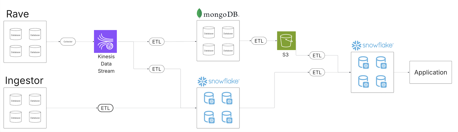
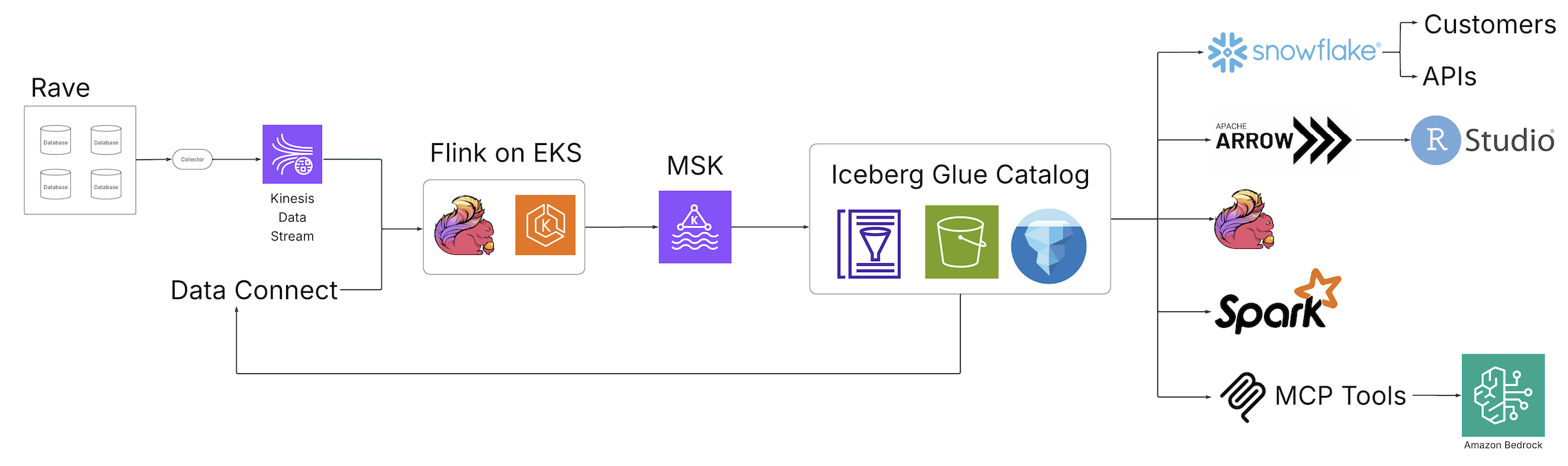
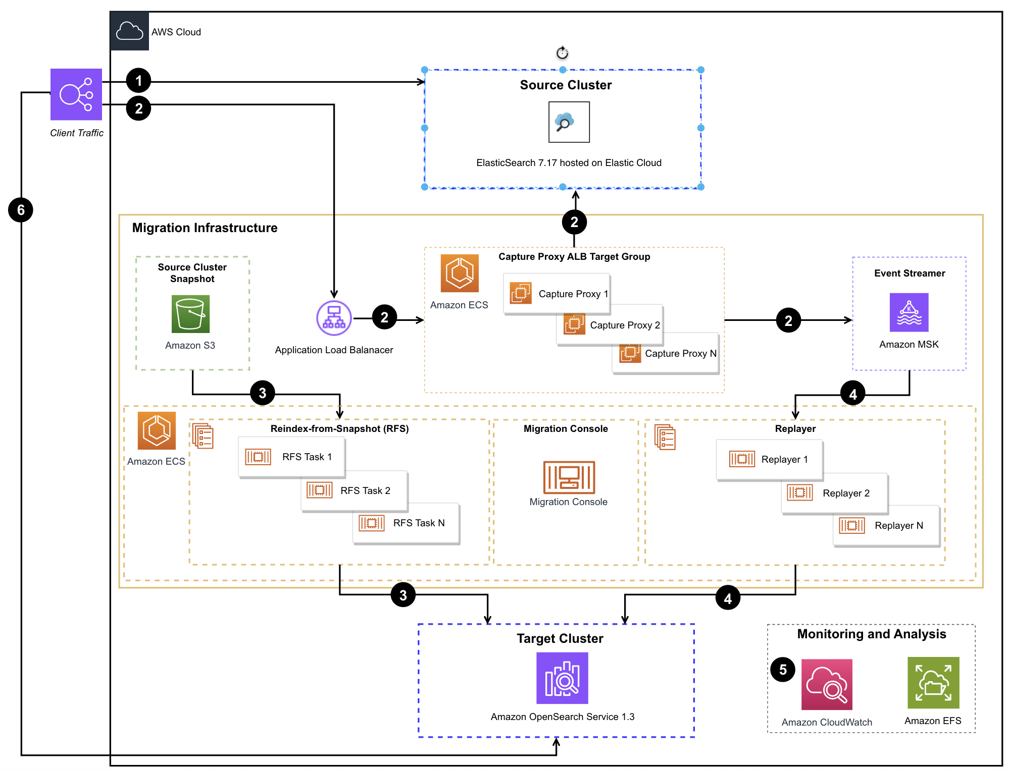
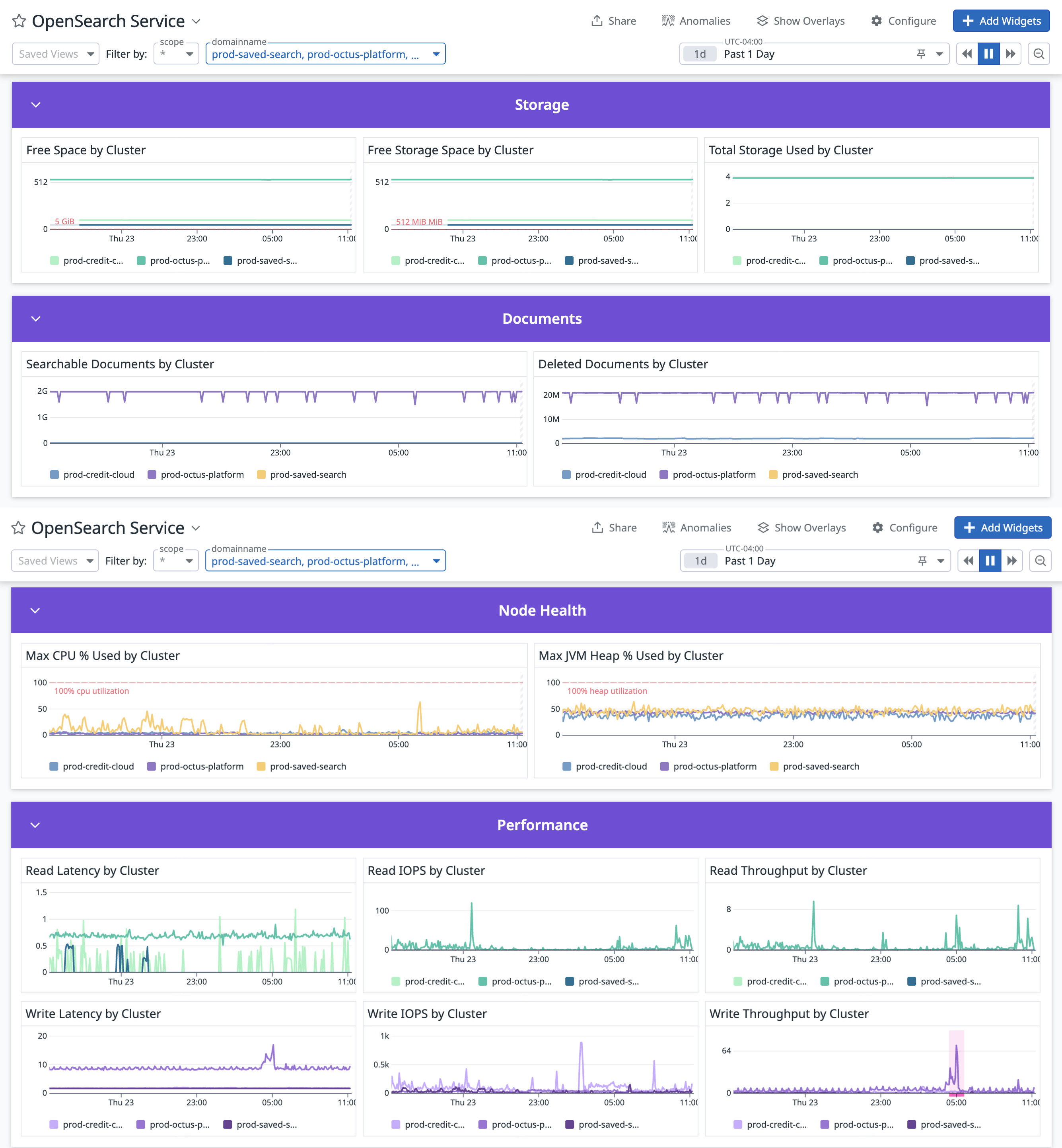
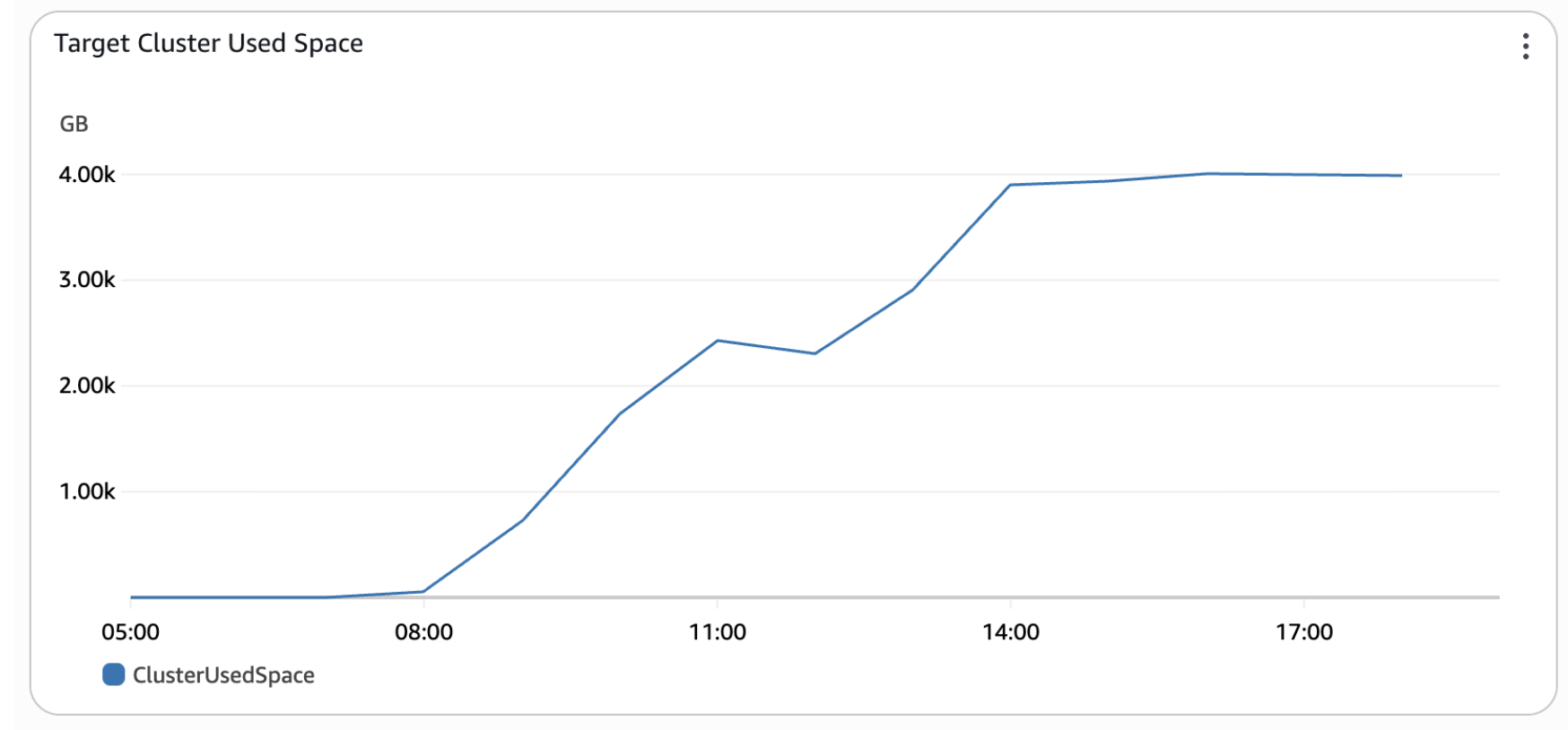
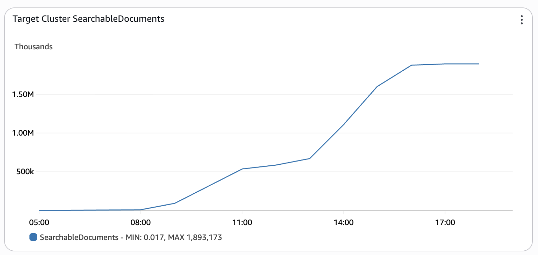
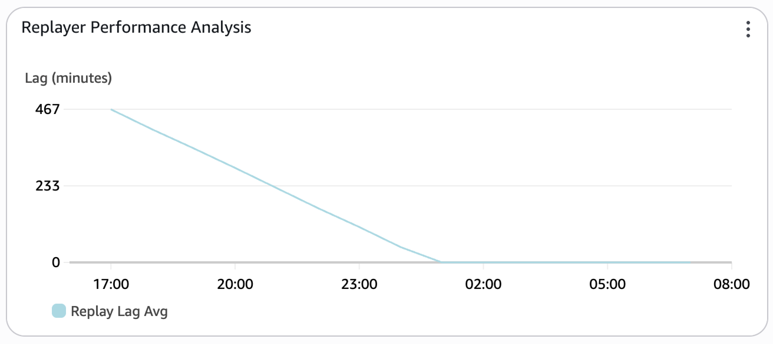
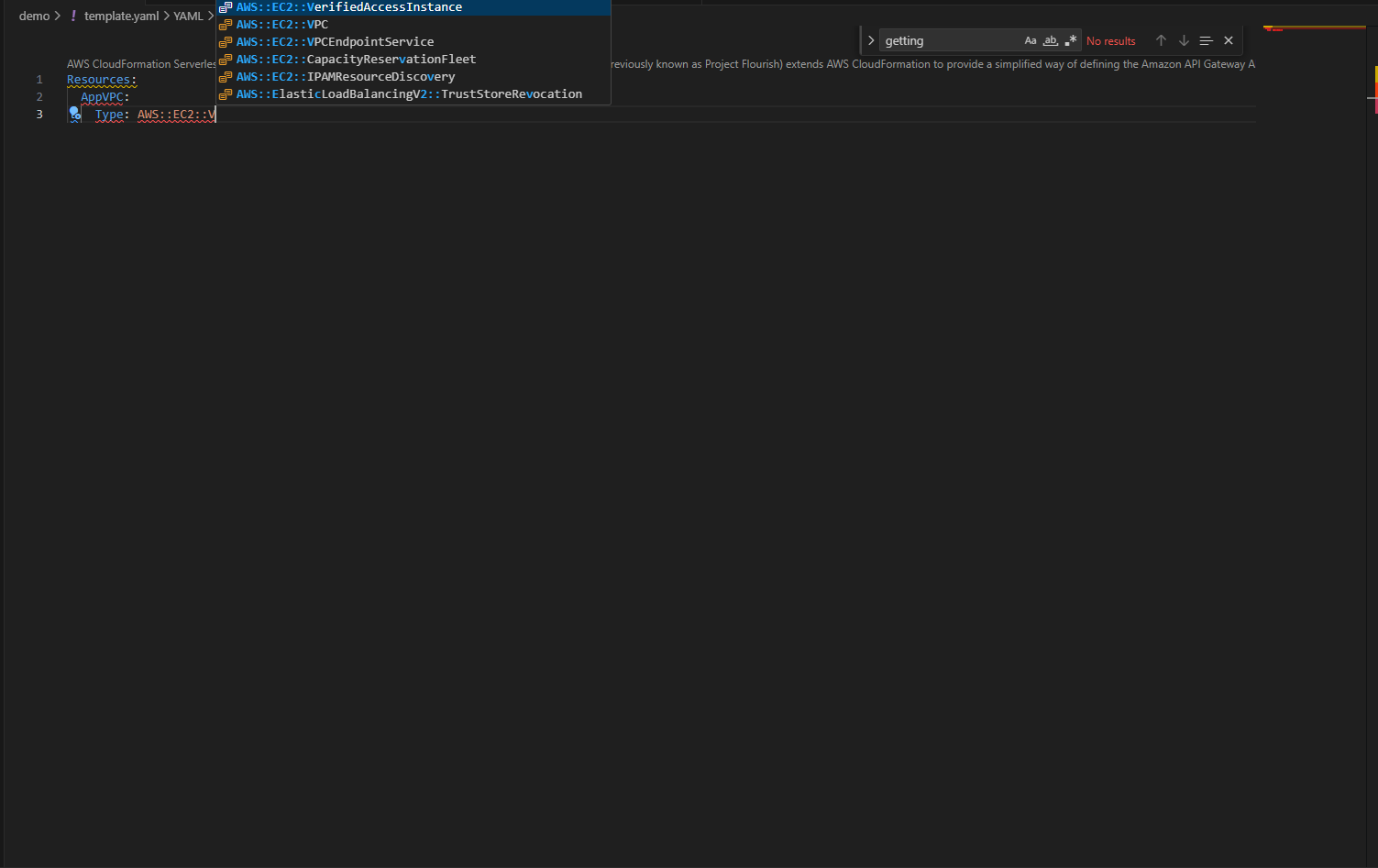
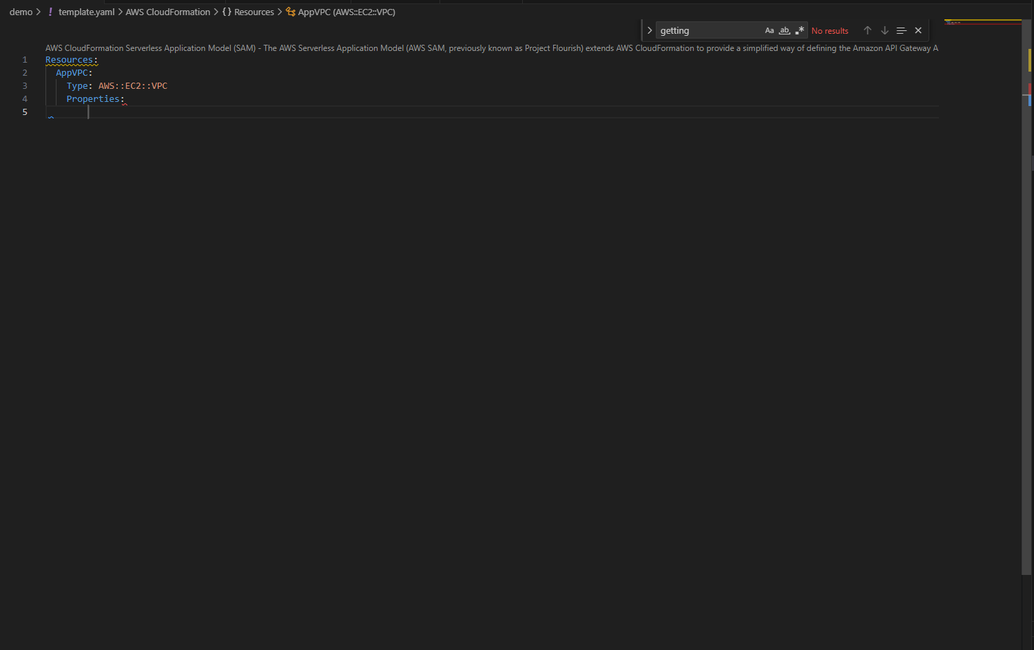

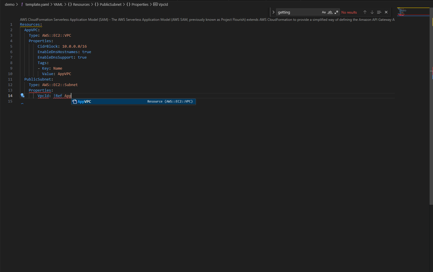
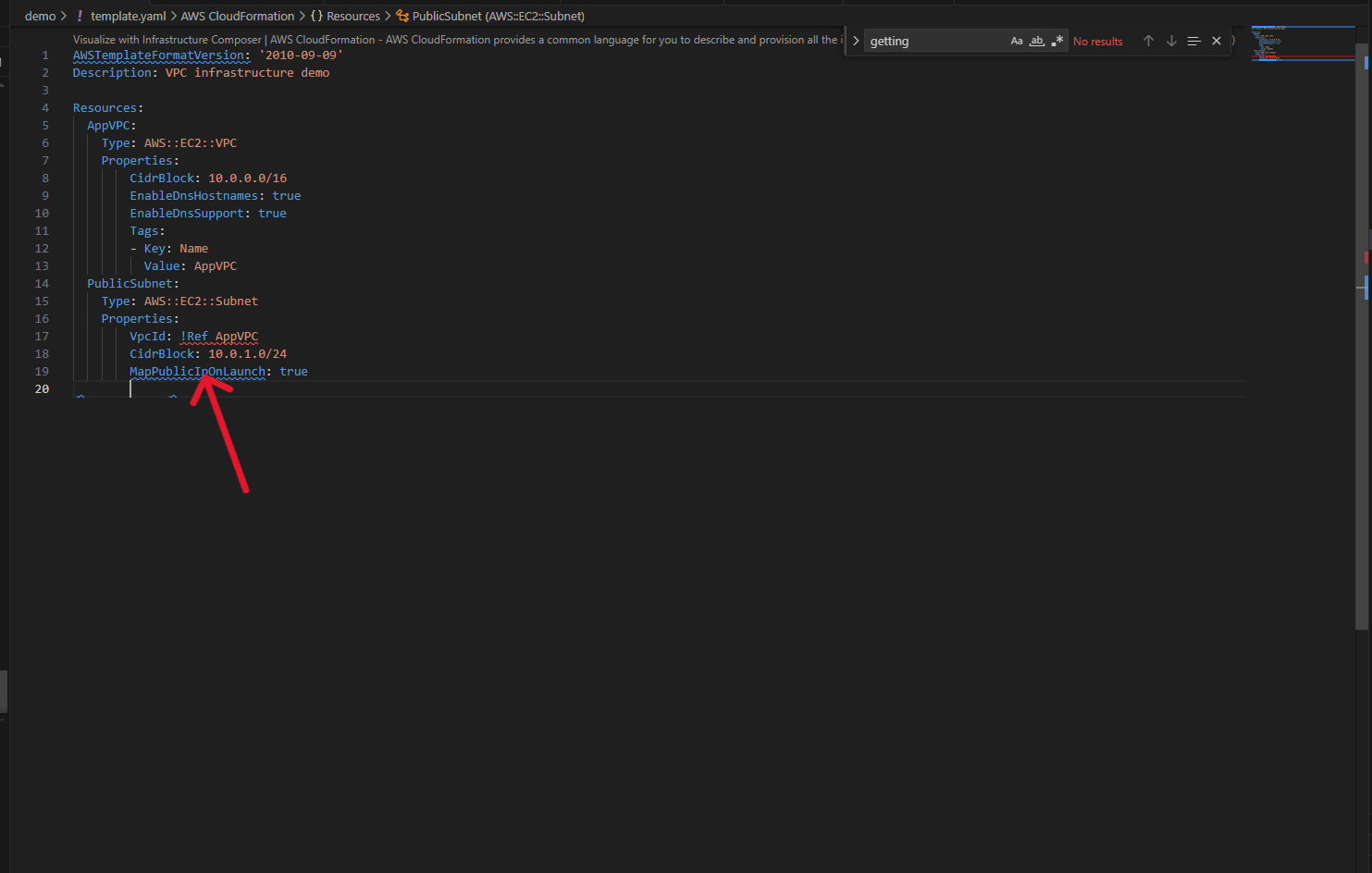
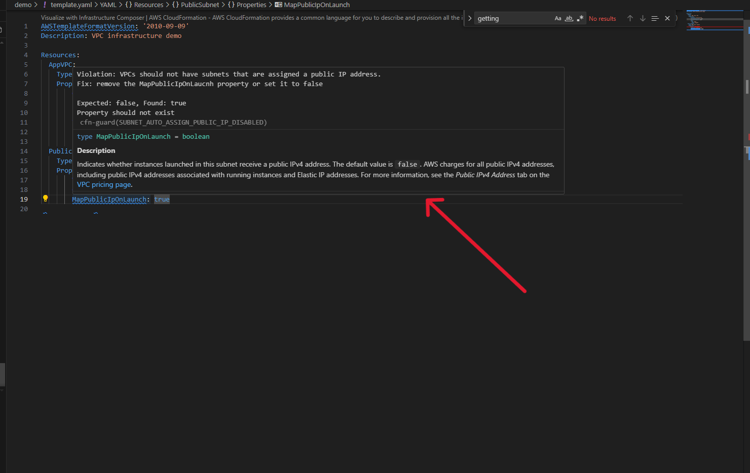
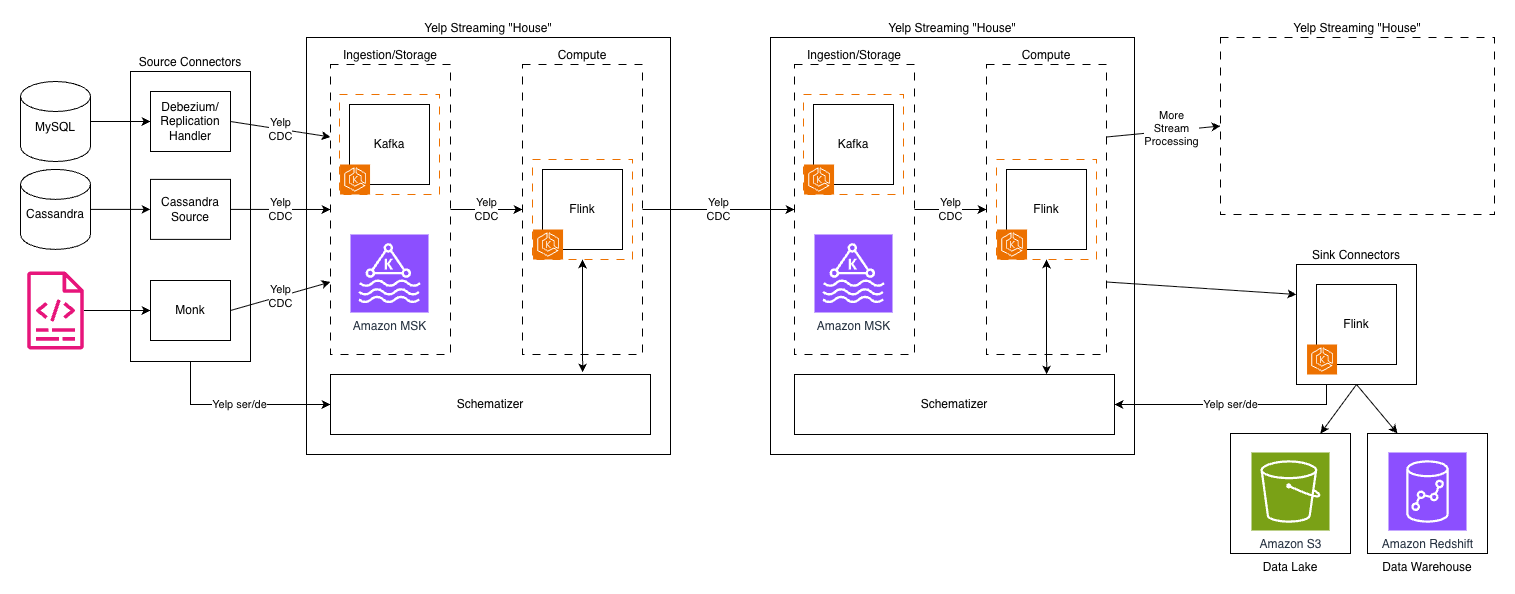
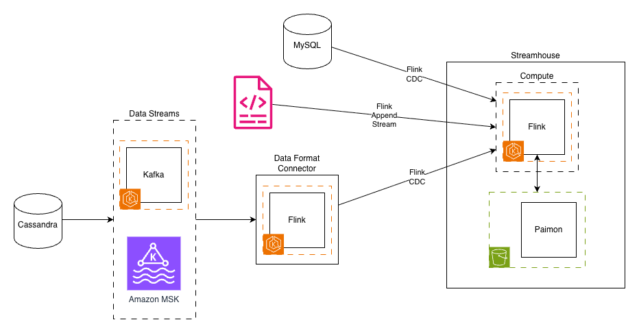
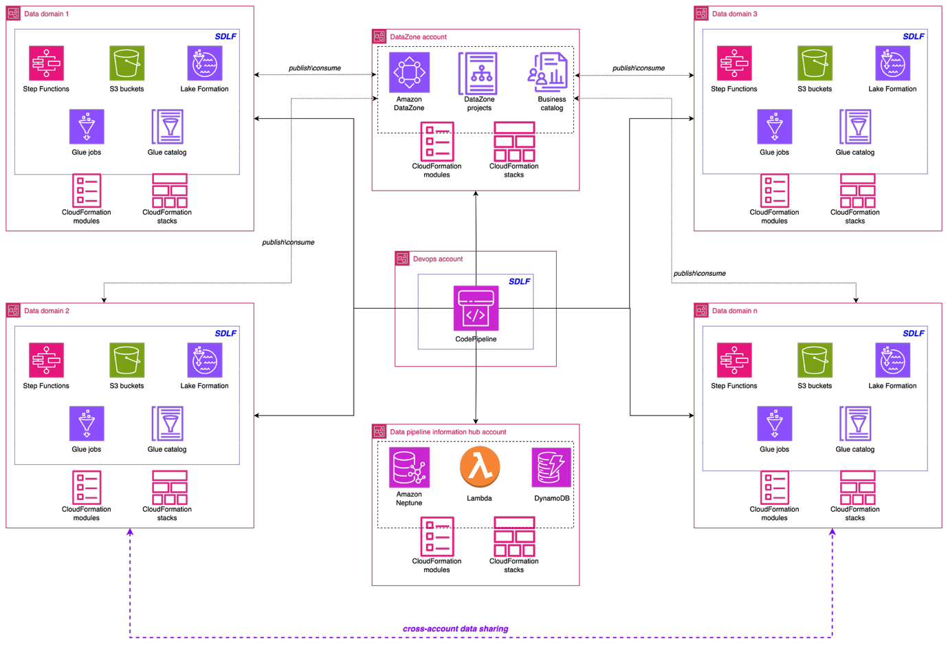
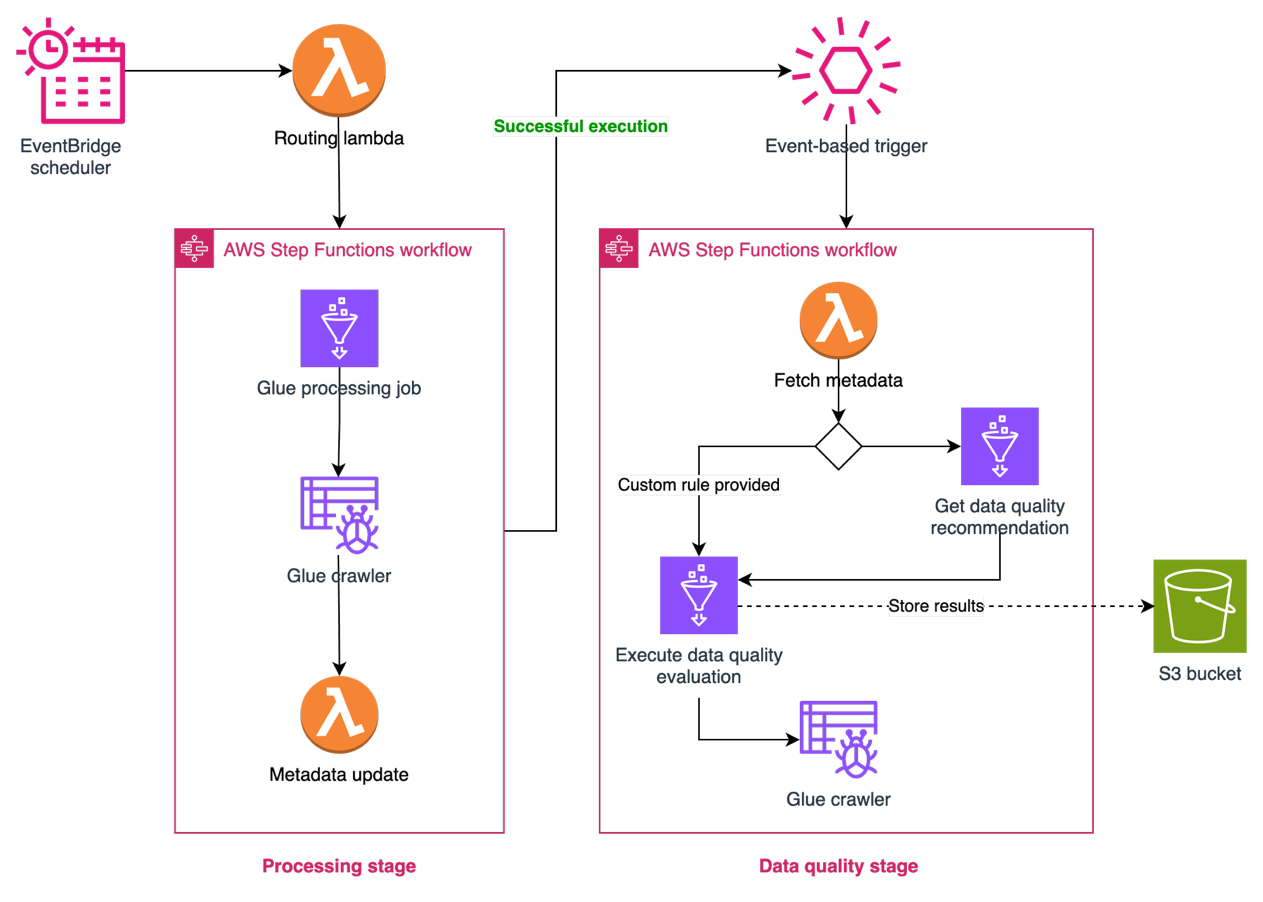
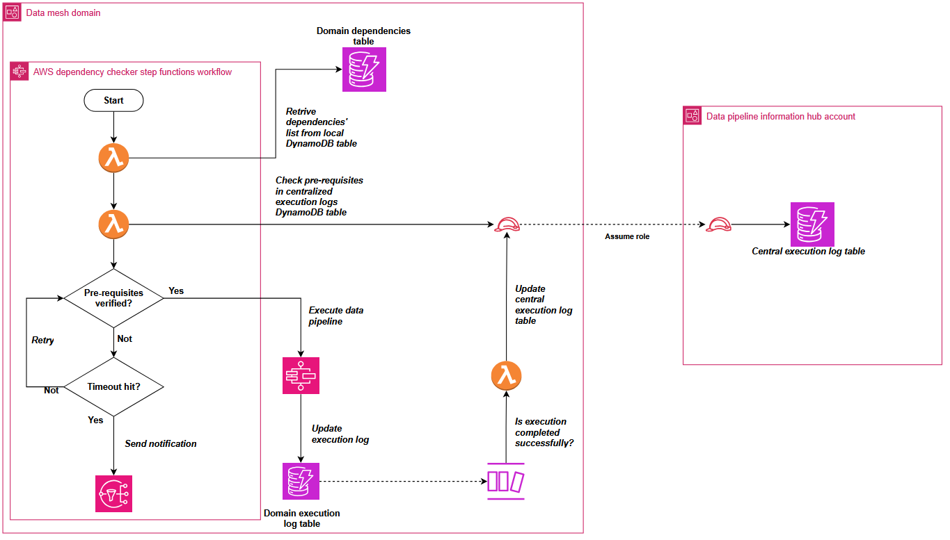
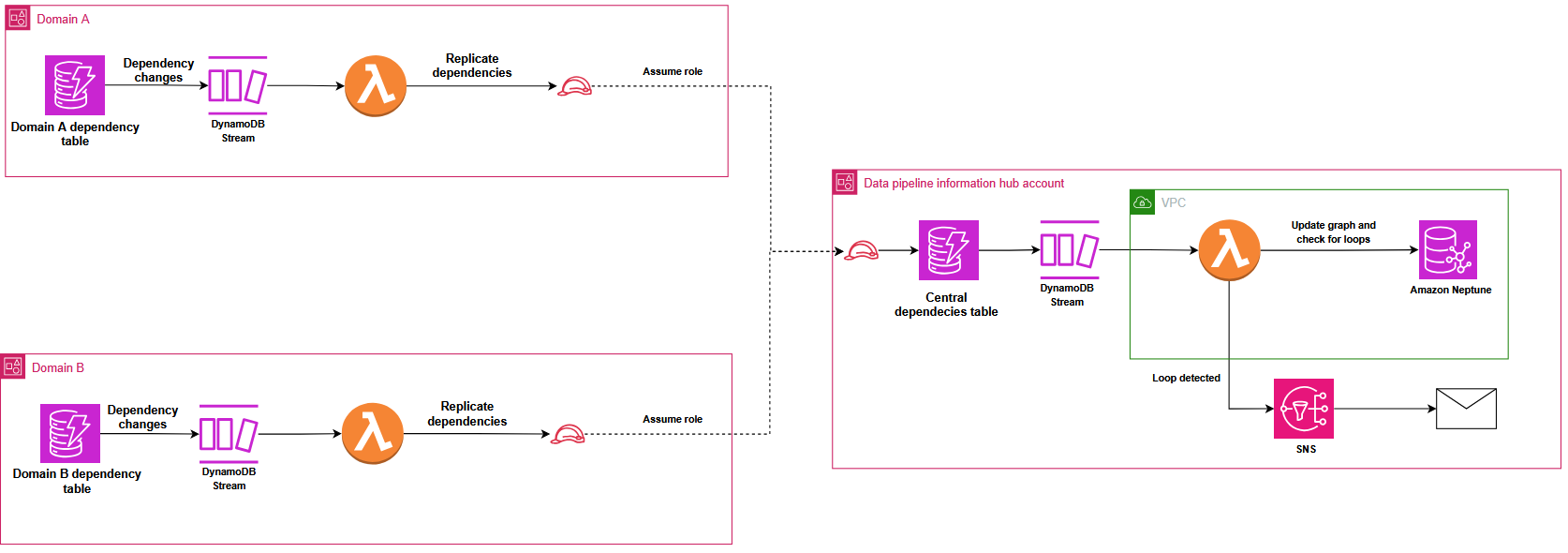
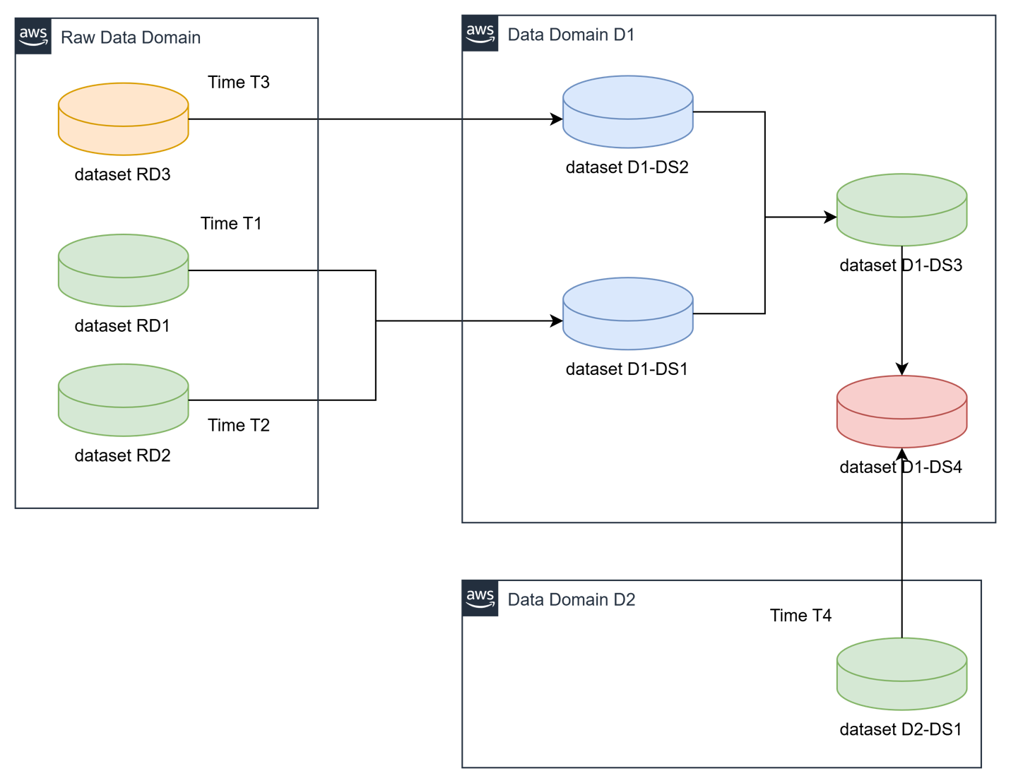
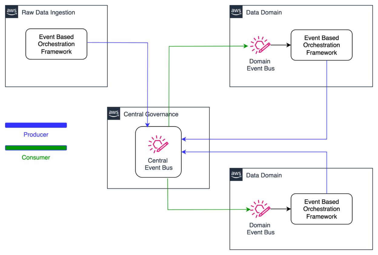
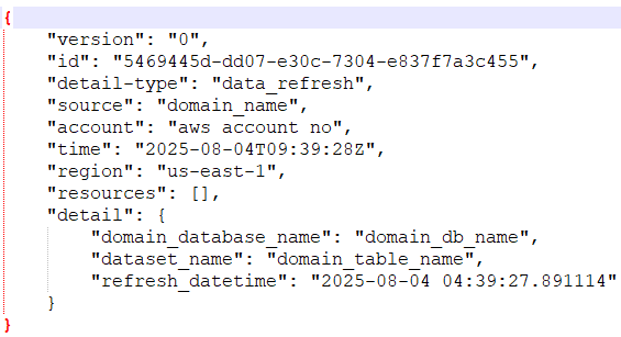
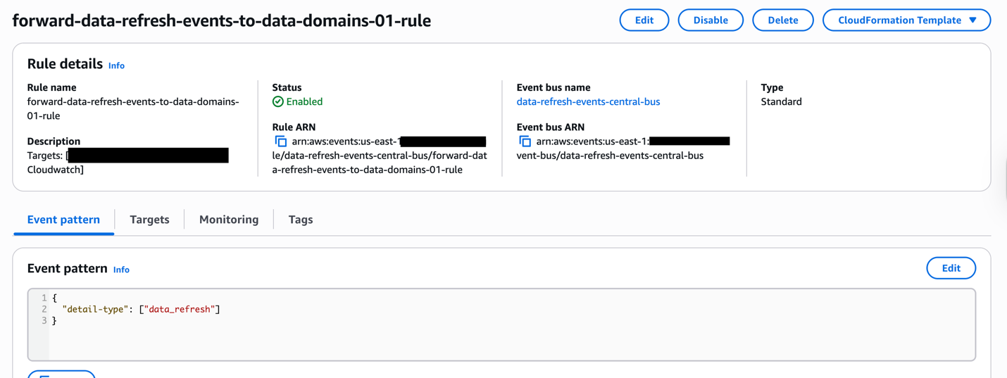
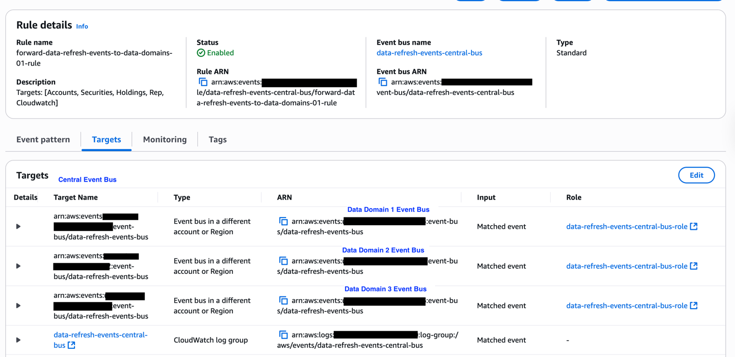
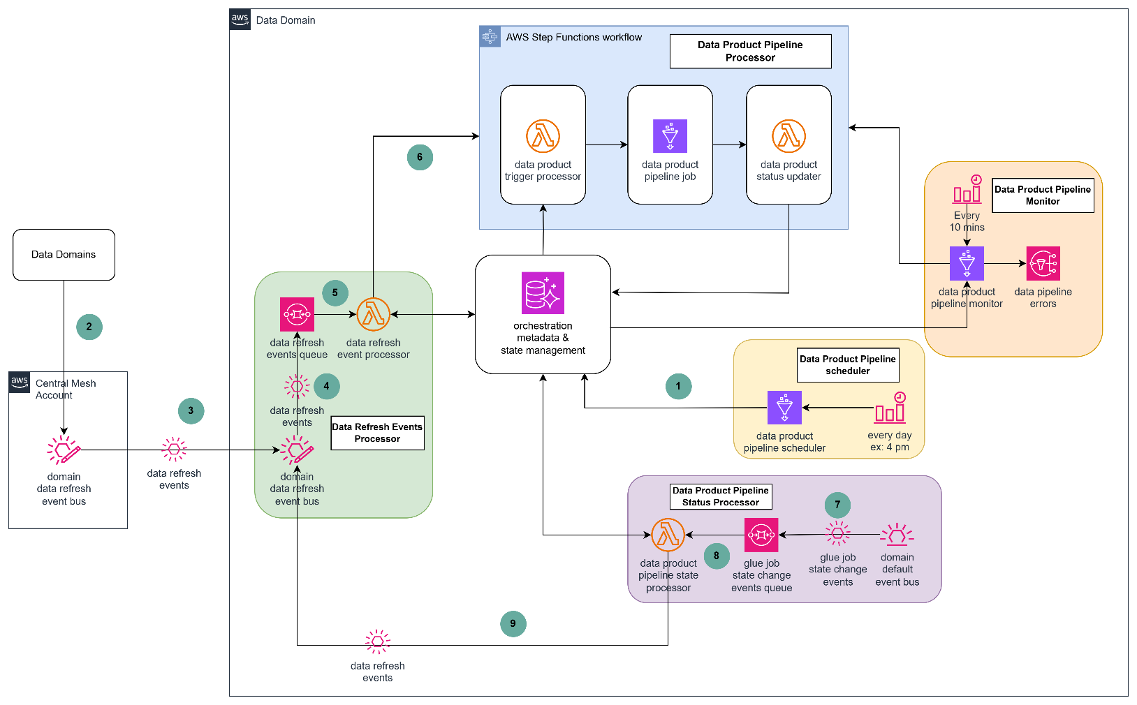
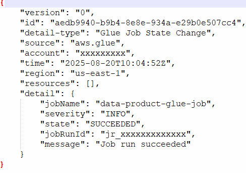
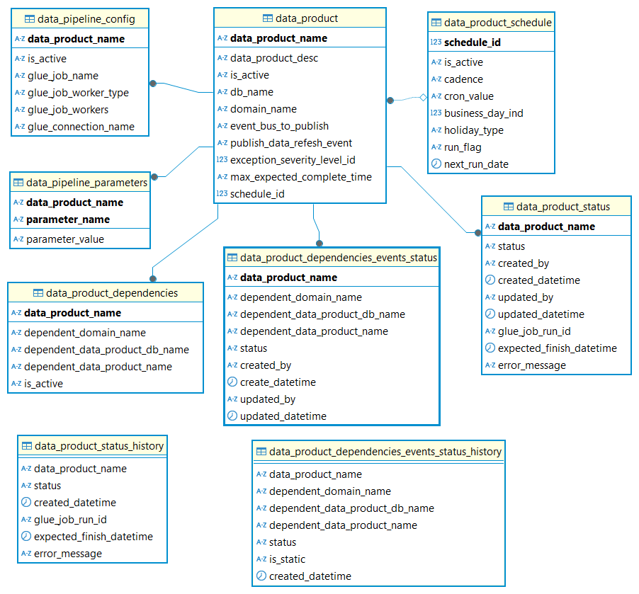
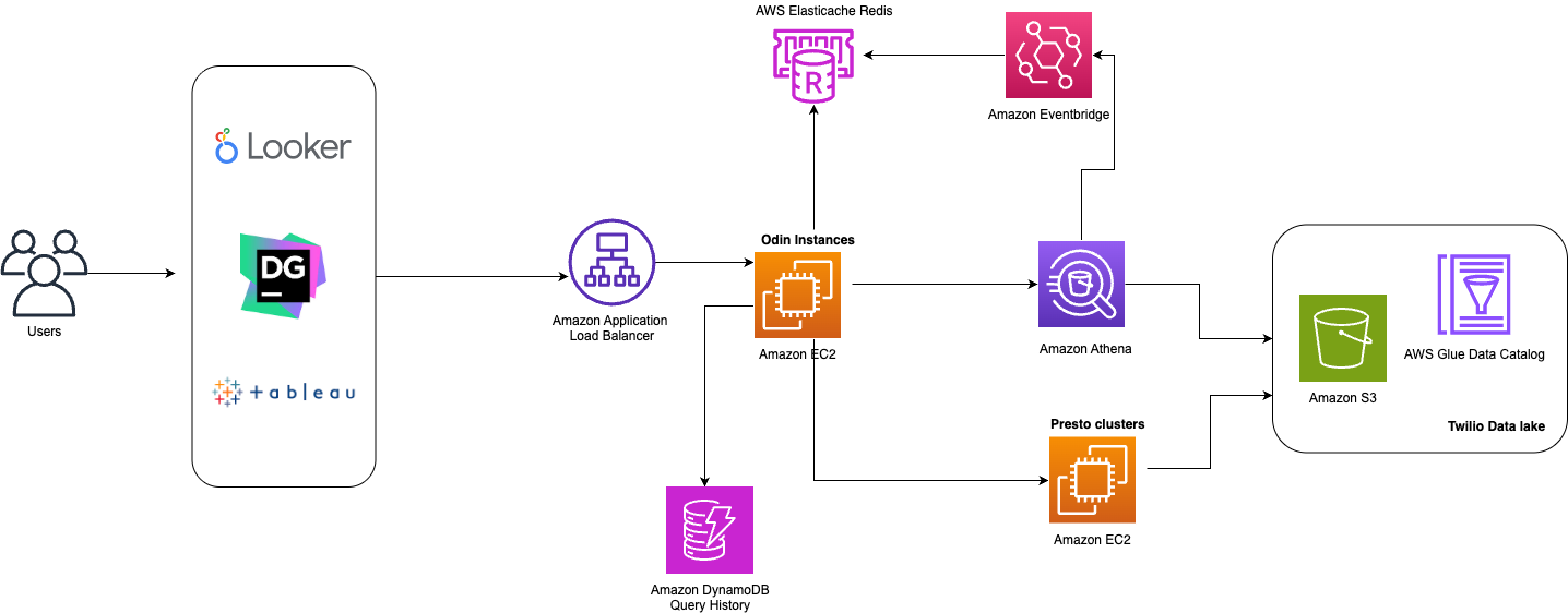
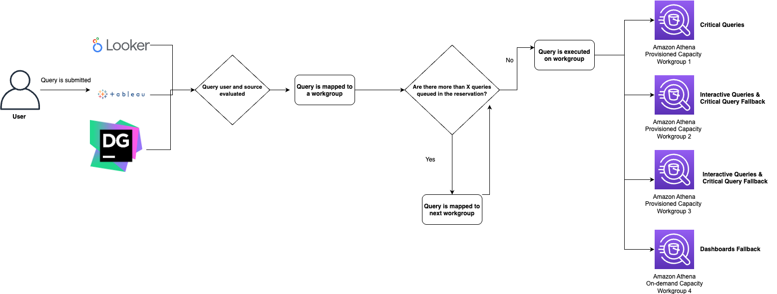
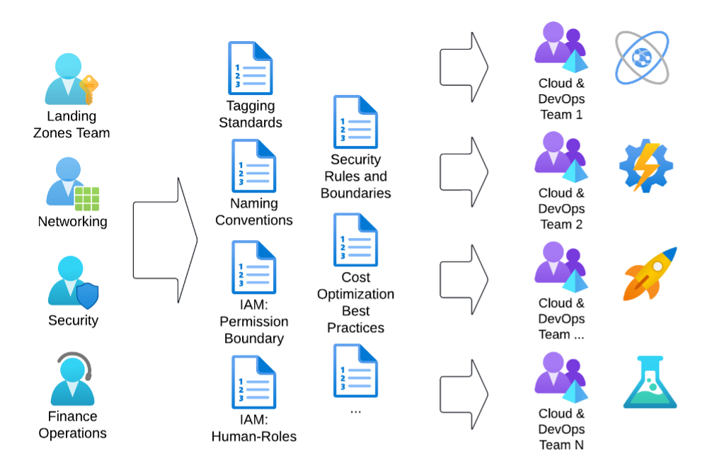
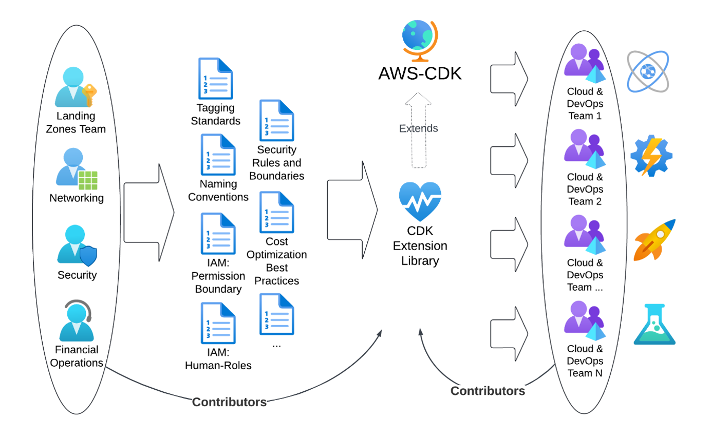
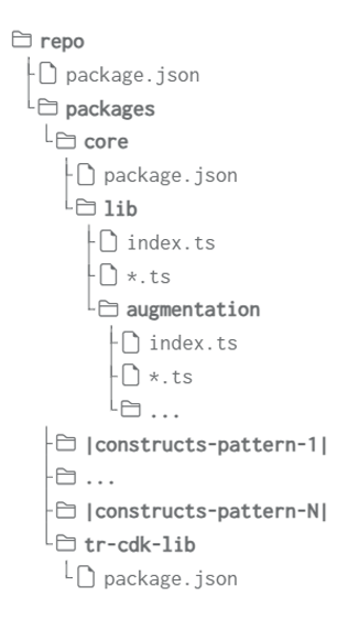
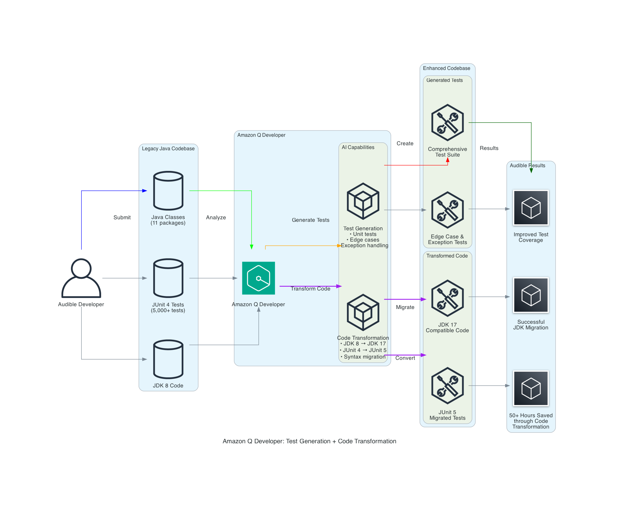
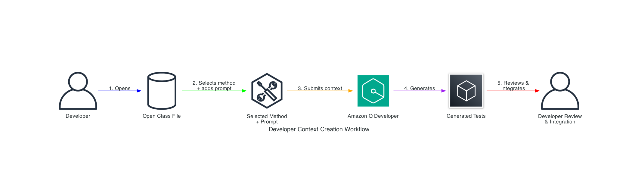


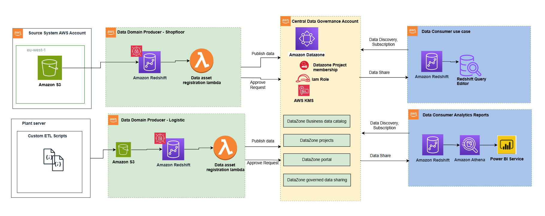
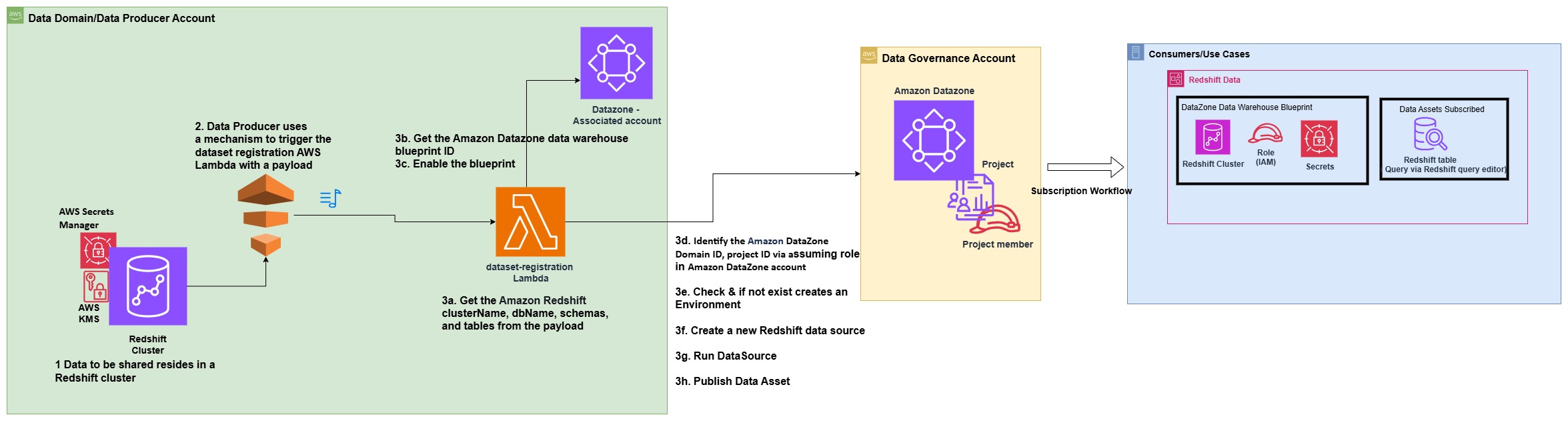
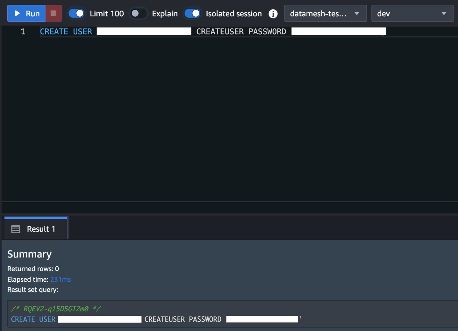
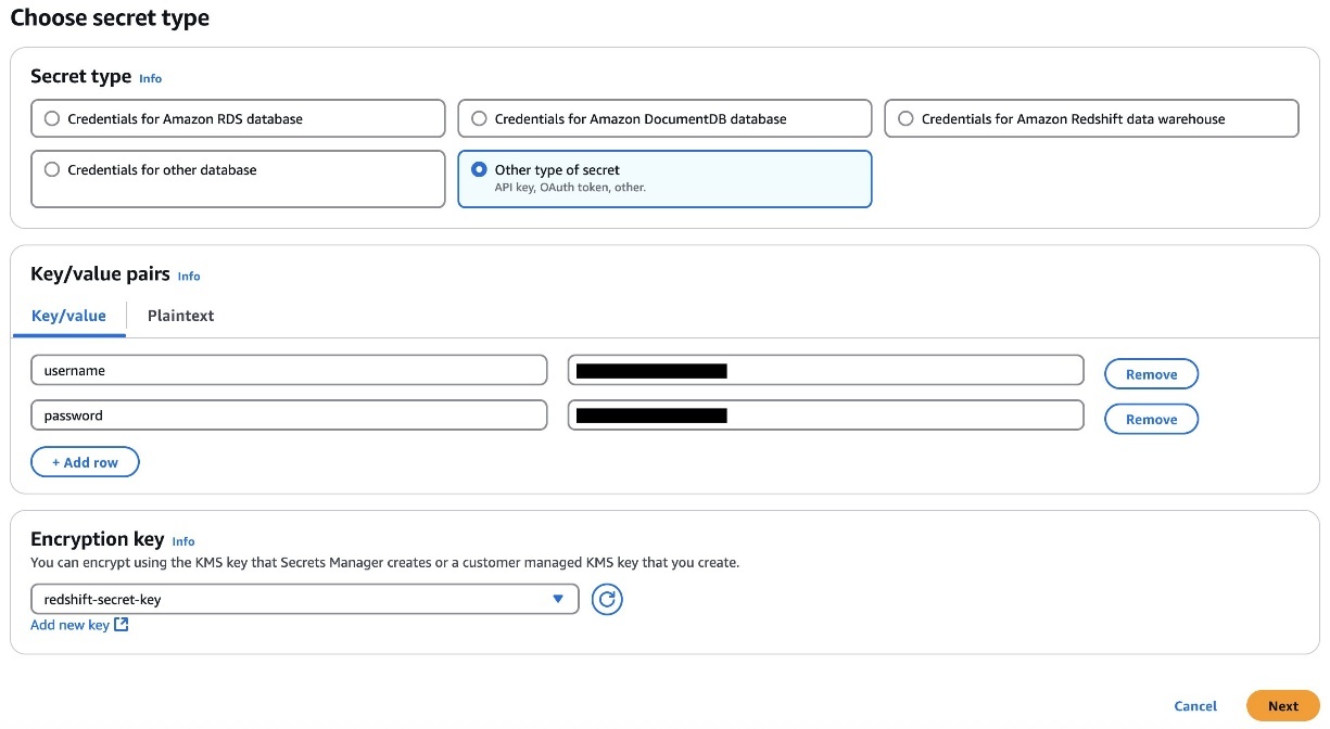
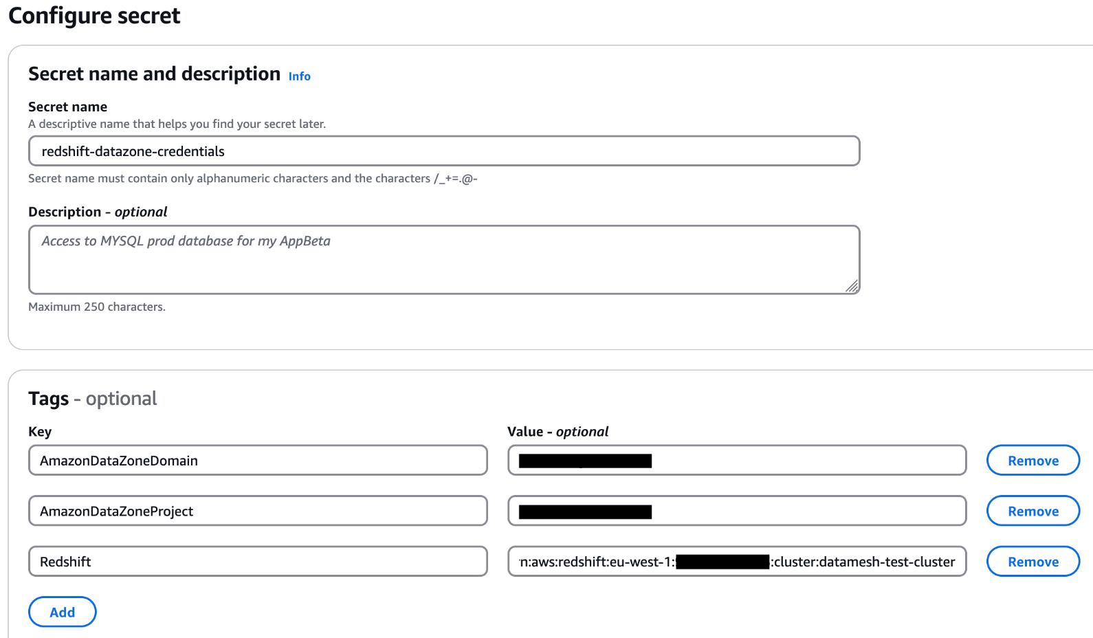
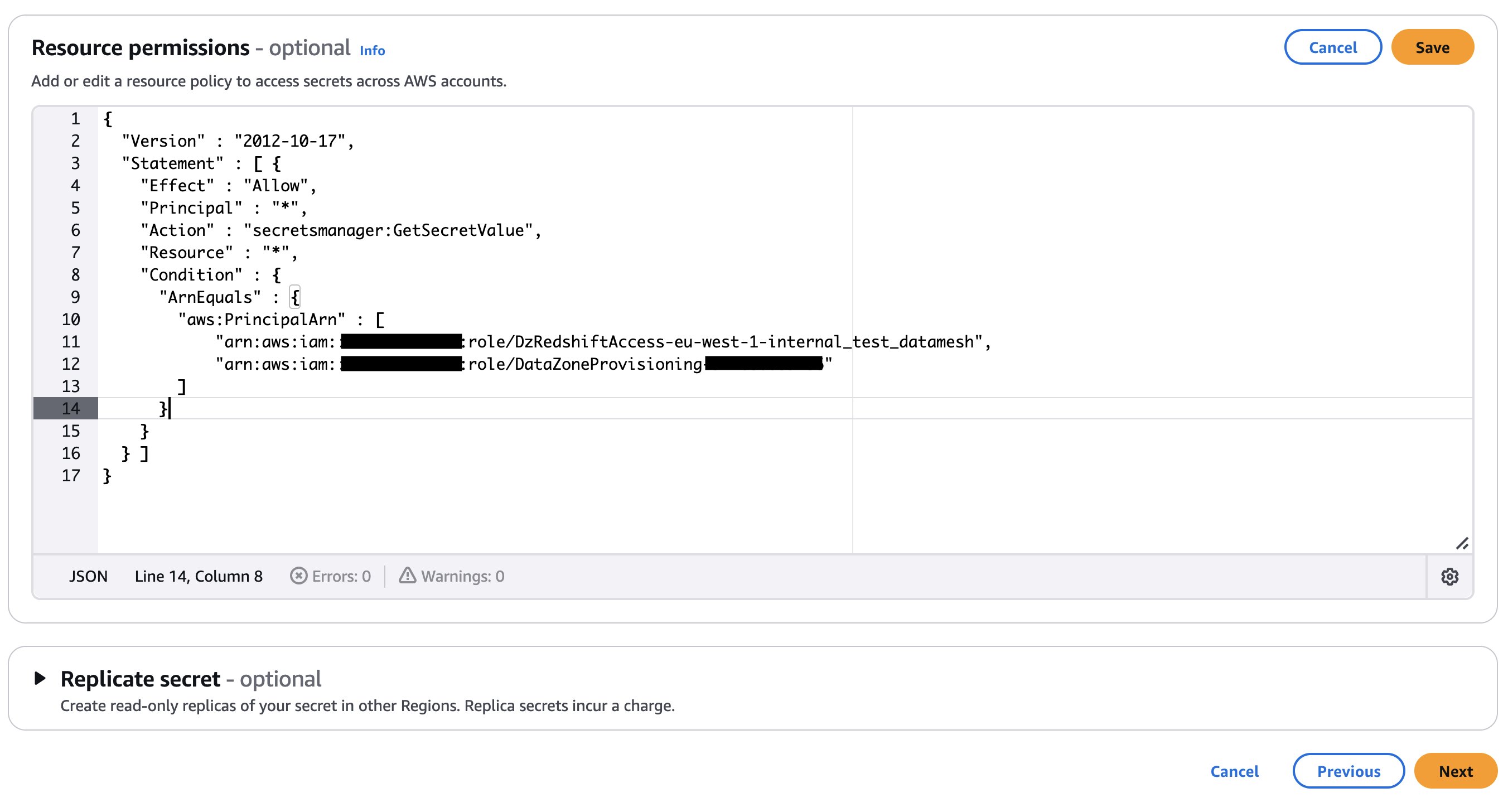 If your secret is encrypted with a custom KMS key, append the key policy with the following statement and add a tag to the key:
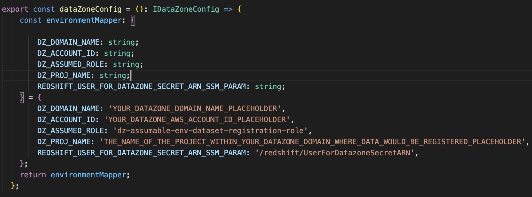
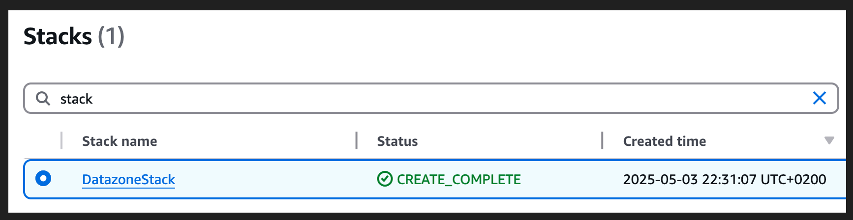
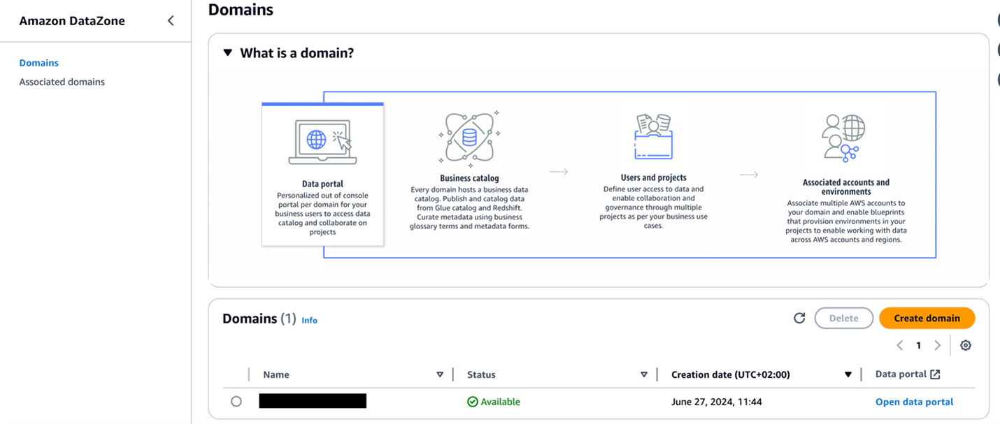
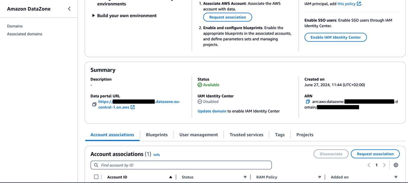

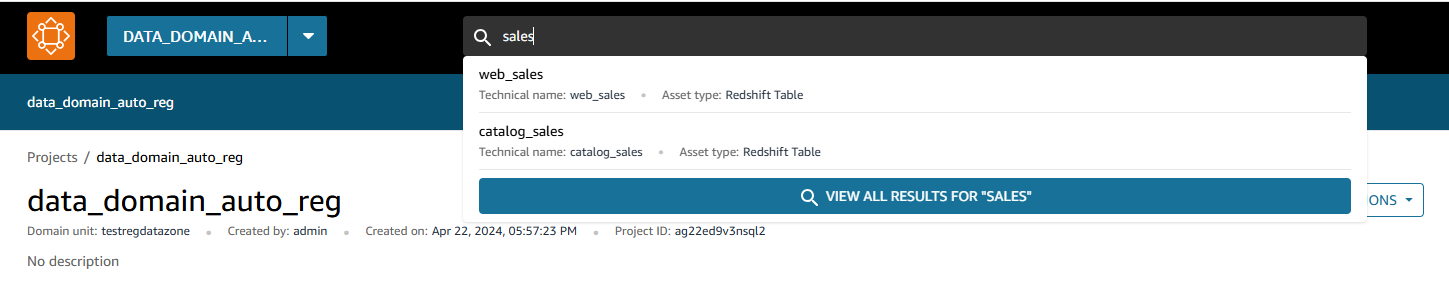
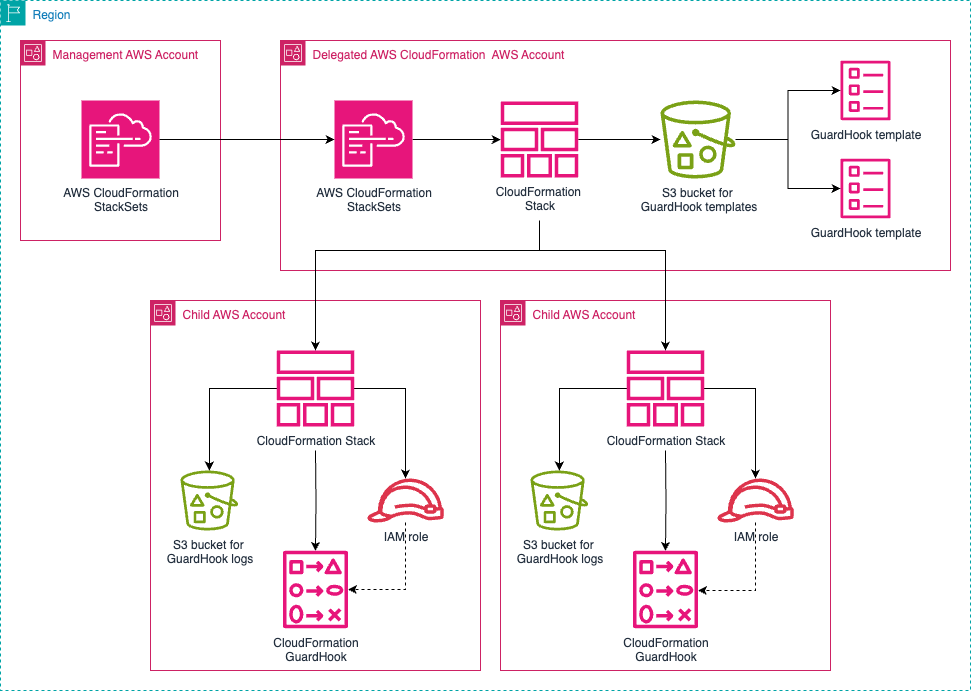
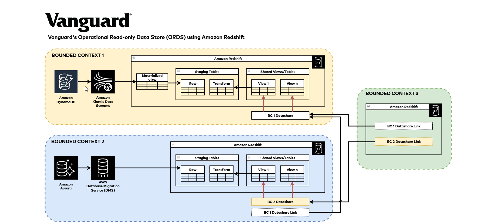
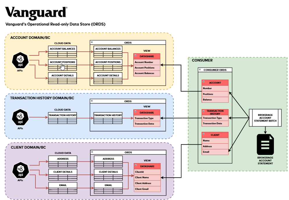

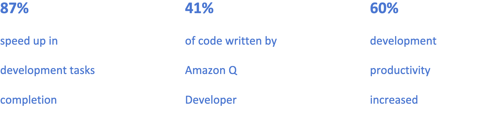
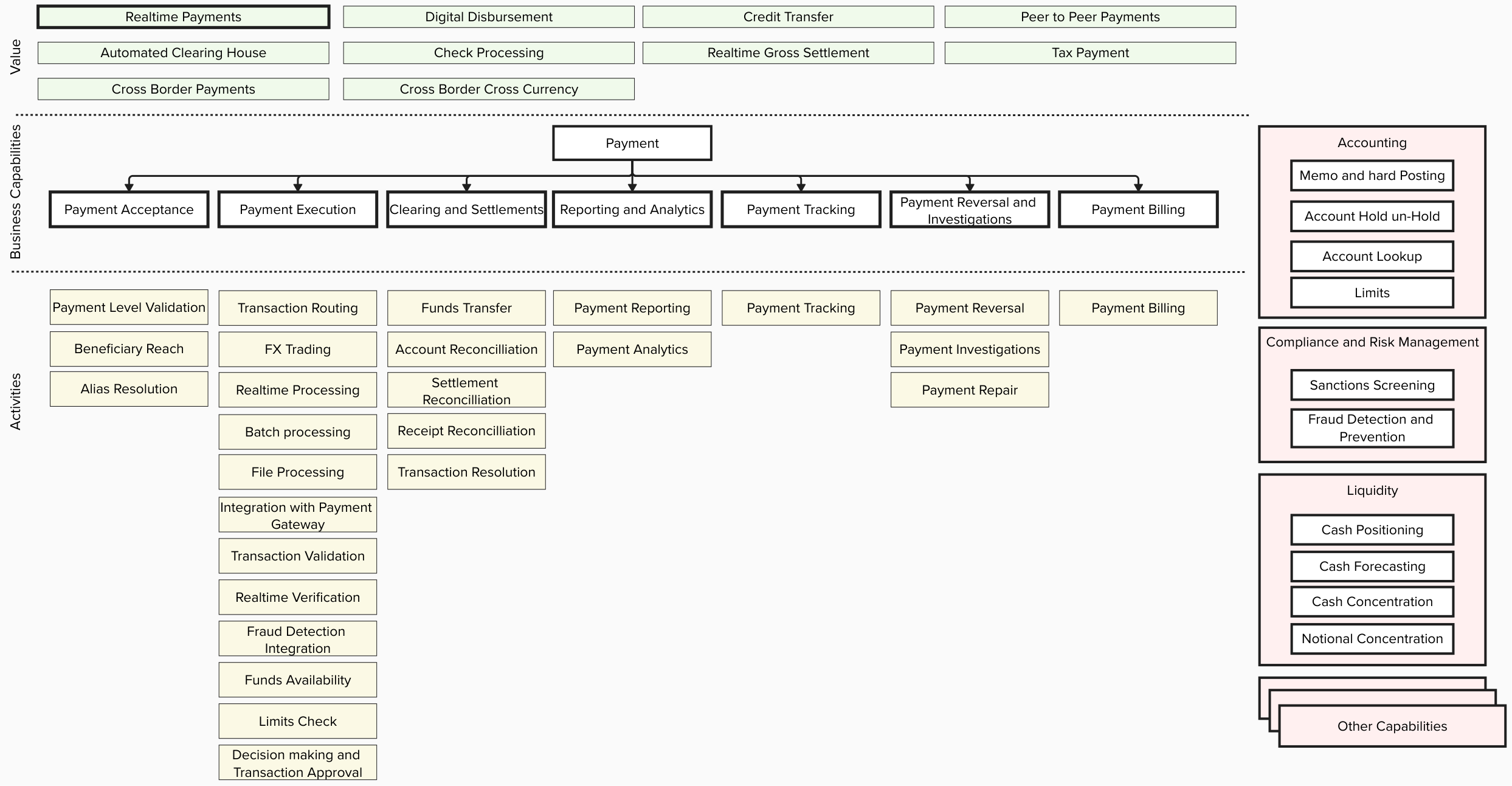
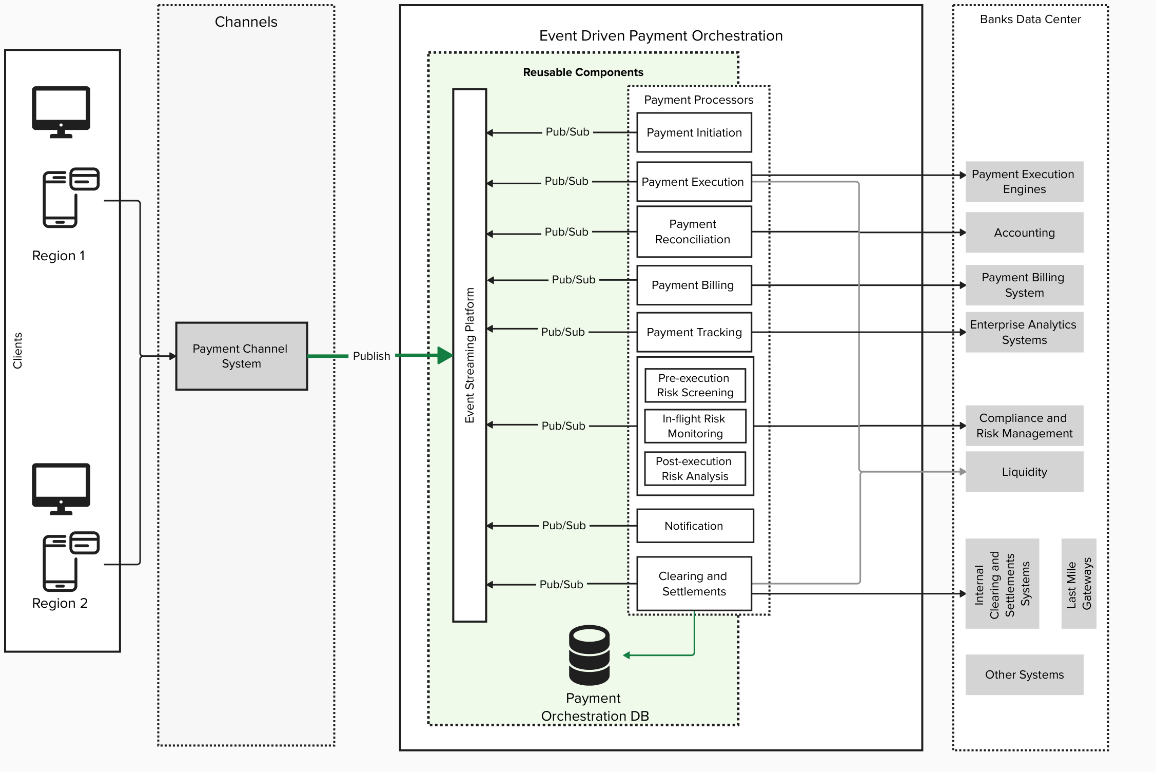
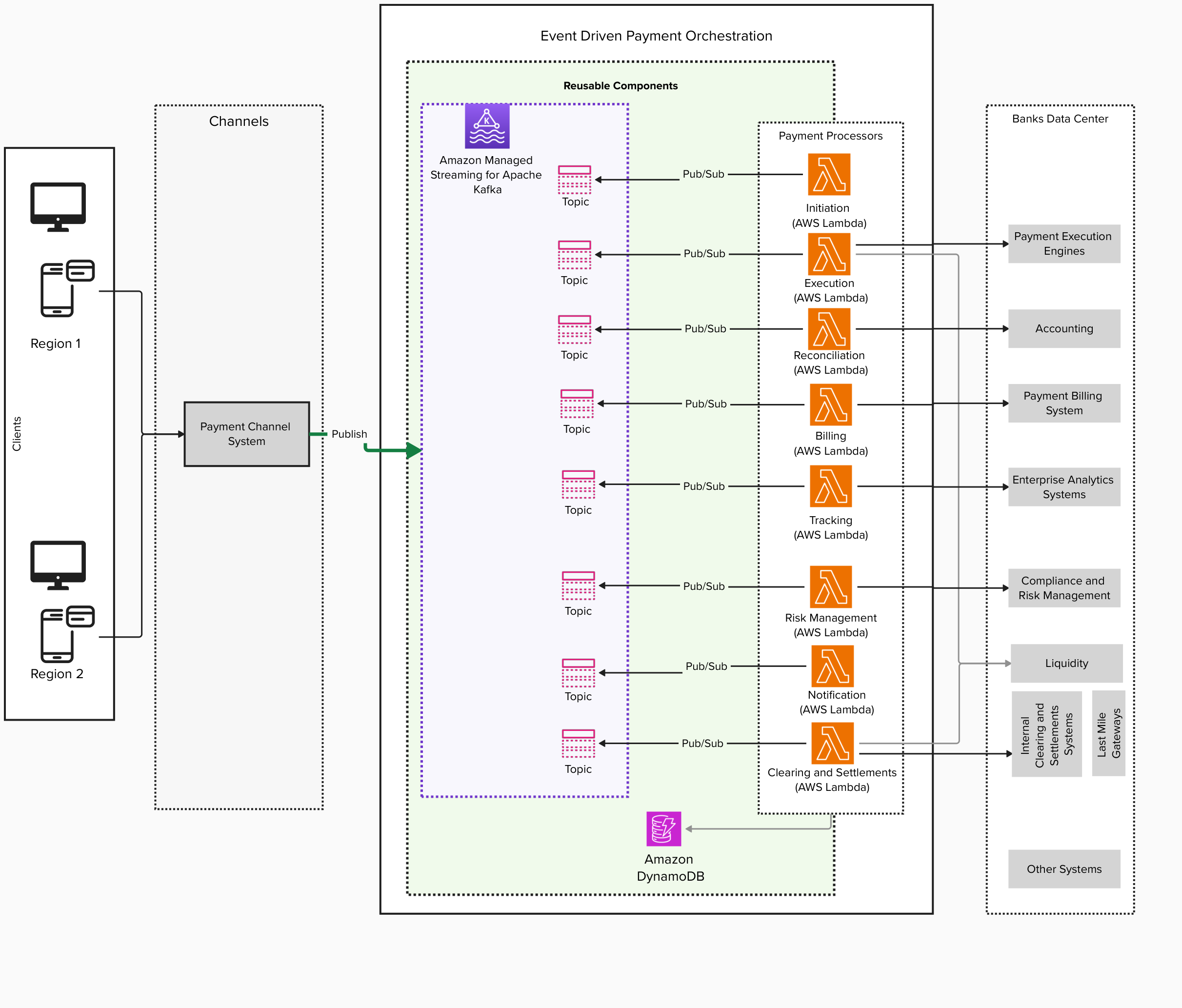
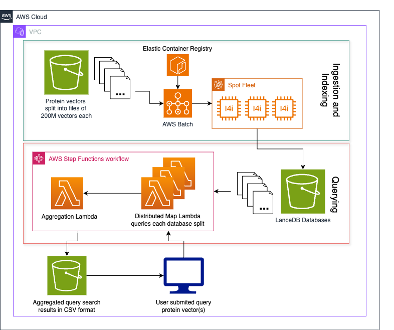
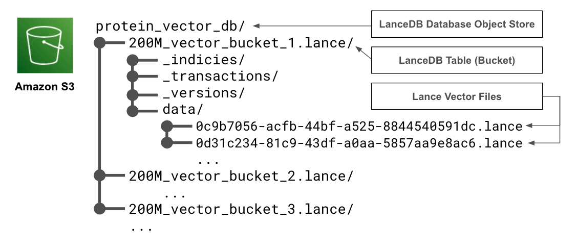
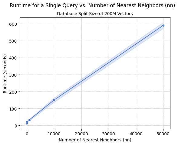
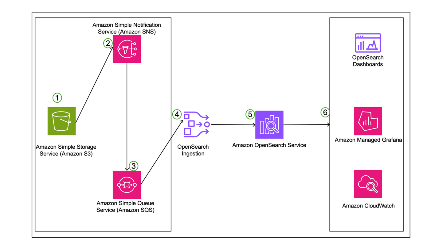
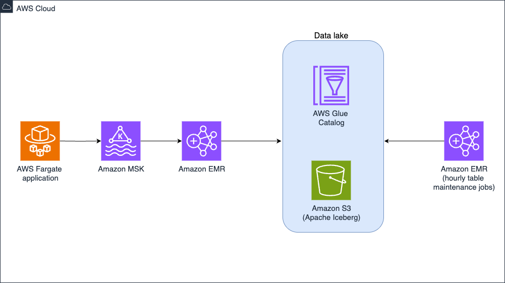
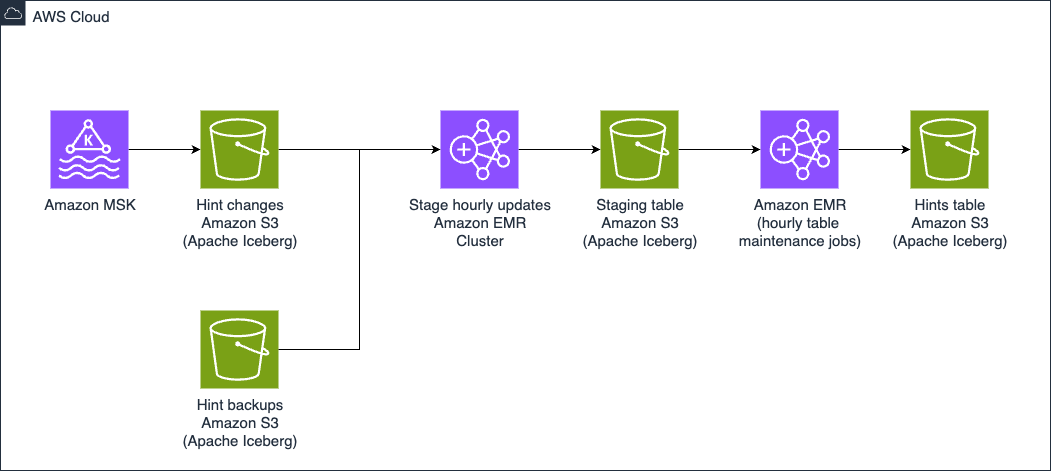
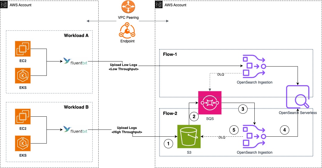
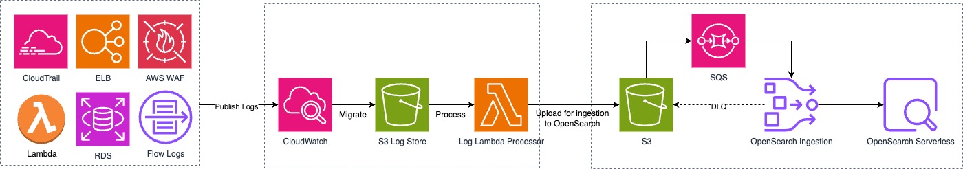
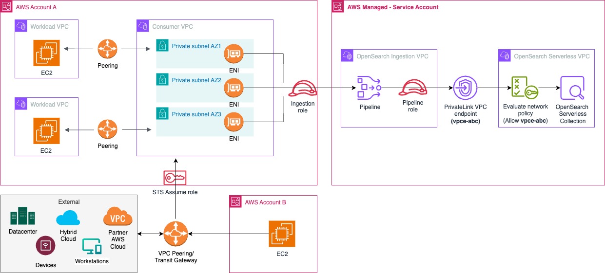
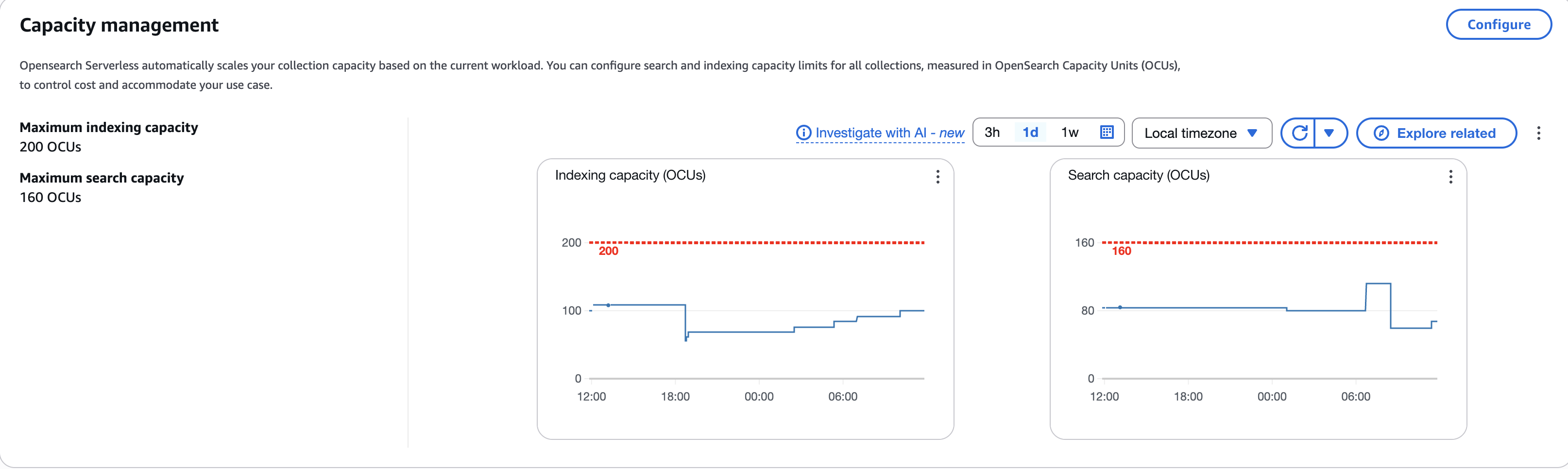
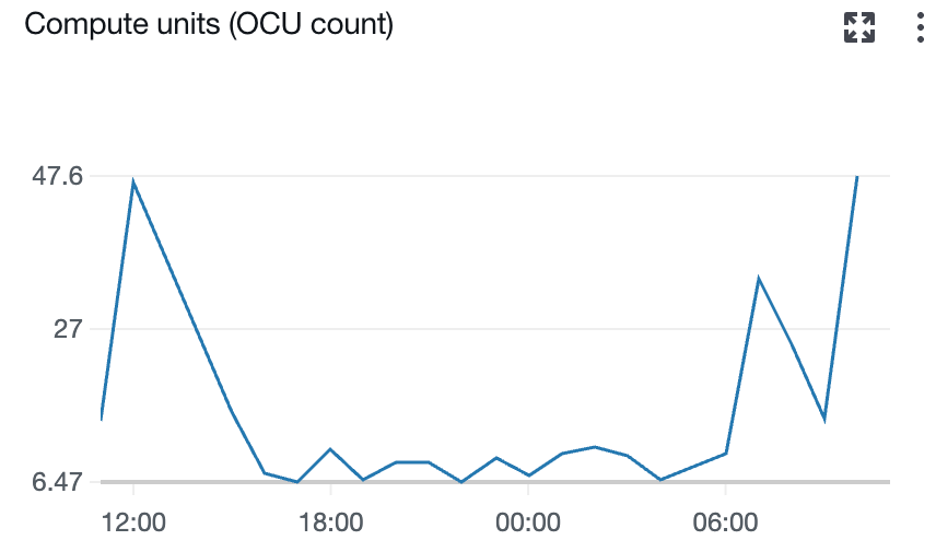
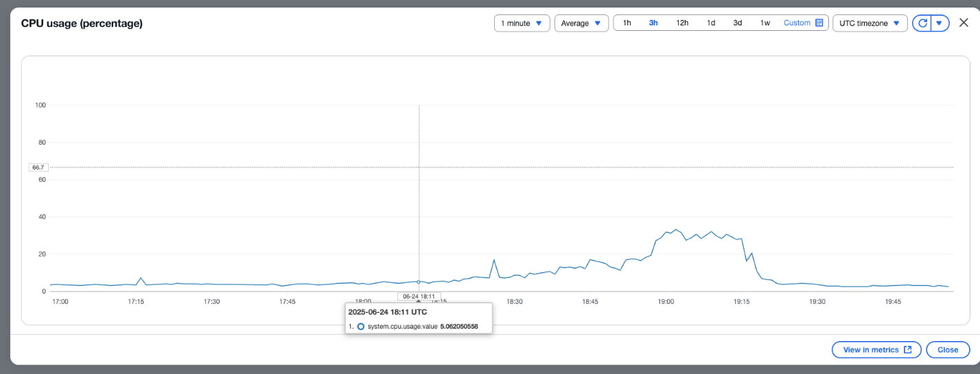
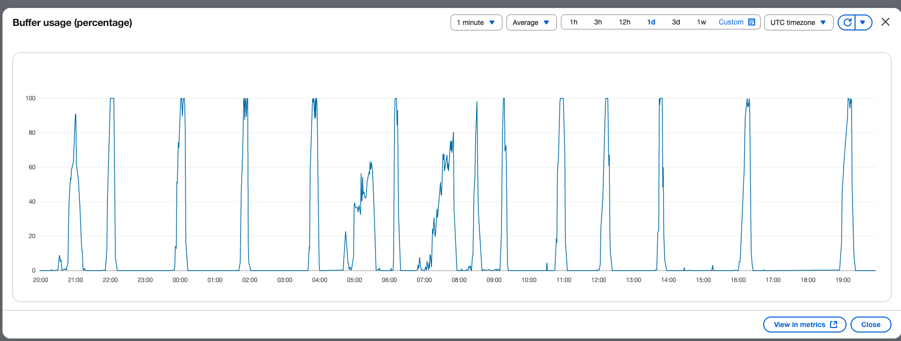
 Prashanth Dudipala is a DevOps Architect at AppZen, where he helps build scalable, secure, and automated cloud platforms on AWS. He’s passionate about simplifying complex systems, enabling teams to move faster, and sharing practical insights with the cloud community.
 Madhuri Andhale is a DevOps Engineer at AppZen, focused on building and optimizing cloud-native infrastructure. She is passionate about managing efficient CI/CD pipelines, streamlining infrastructure and deployments, modernizing systems, and enabling development teams to deliver faster and more reliably. Outside of work, Madhuri enjoys exploring emerging technologies, traveling to new places, experimenting with new recipes, and finding creative ways to solve everyday challenges.
 Manoj Gupta is a Senior Solutions Architect at AWS, based in San Francisco. With over 4 years of experience at AWS, he works closely with customers like AppZen to build optimized cloud architectures. His primary focus areas are Data, AI/ML, and Security, helping organizations modernize their technology stacks. Outside of work, he enjoys outdoor activities and traveling with family.
 Prashant Agrawal is a Sr. Search Specialist Solutions Architect with Amazon OpenSearch Service. He works closely with customers to help them migrate their workloads to the cloud and helps existing customers fine-tune their clusters to achieve better performance and save on cost. Before joining AWS, he helped various customers use OpenSearch and Elasticsearch for their search and log analytics use cases. When not working, you can find him traveling and exploring new places. In short, he likes doing Eat → Travel → Repeat.