Post Syndicated from Angel Conde Manjon original https://aws.amazon.com/blogs/big-data/compaction-support-for-avro-and-orc-file-formats-in-apache-iceberg-tables-in-amazon-s3/
Apache Iceberg, a high-performance open table format (OTF), has gained widespread adoption among organizations managing large scale analytic tables and data volumes. Iceberg brings the reliability and simplicity of SQL tables to data lakes while enabling engines like Apache Spark, Apache Trino, Apache Flink, Apache Presto, Apache Hive, Apache Impala, and AWS analytic services like Amazon Athena to flexibly and securely access data with lakehouse architecture. While the lakehouse built using Iceberg represents an evolution to the data lake, but it still requires services to compact and optimize the files and partitions that comprise the tables. Self-managing Iceberg tables with large volumes of data poses several challenges, including managing concurrent transactions, processing real-time data streams, handling small file proliferation, maintaining data quality and governance, and ensuring compliance.
At re:Invent 2024, Amazon S3 introduced Amazon S3 Tables marking the first cloud object store with native Iceberg support for Parquet files, designed to streamline tabular data management at scale. Parquet is one of the most common and fastest growing data types in Amazon S3. Amazon S3 stores exabytes of Parquet data, and averages over 15 million requests per second to this data. While S3 Tables initially supported Parquet file type, as discussed in the S3 Tables AWS News Blog, the Iceberg specification extends to Avro, and ORC file formats for managing large analytic tables. Now, S3 Tables is expanding its capabilities to include automatic compaction for these additional file types within Iceberg tables. This enhancement is also available for Iceberg tables on general purpose S3 buckets, using the lakehouse architecture of Amazon SageMaker that previously supported Parquet compaction as covered in the blog post Accelerate queries on Apache Iceberg tables through AWS Glue auto compaction.
This blog post explores the performance benefits of automatic compaction of Iceberg tables using Avro and ORC file types in S3 Tables for a data ingestion use with over 20 billion events.
Parquet, ORC, and Avro file formats
Parquet is one of the most common and fastest growing data types in Amazon S3. It was originally developed by Twitter and now part of the Apache ecosystem, is known for its broad compatibility with big data tools such as Spark, Hive, Impala, and Drill. Amazon S3 stores exabytes of Apache Parquet data, and averages over 15 million requests per second to this data. Parquet uses a hybrid encoding scheme and supports complex nested data structures, making it ideal for read-heavy workloads and analytics across various platforms. Parquet also provides excellent compression and efficient I/O by enabling selective column reads, reducing the amount of data scanned during queries.
ORC was specifically designed for Hadoop ecosystem and optimized for Hive. It generally offers better compression ratios and better read performance for certain types of queries due to its lightweight indexing and aggressive predicate pushdown capabilities. ORC includes built-in statistics and supports lightweight indexes, which can accelerate filtering operations significantly. While Parquet offers broader tool compatibility, ORC often outperforms it within Hive-centric environments, especially when dealing with flat data structures and large sequential scans.
Avro file format is usually used in streaming scenarios for its serialization and schema handling capabilities and for its seamless integration with Apache Kafka, offering a powerful combination for handling real-time data streams. For example, for storing and validating streaming data schemas, you have the option of using AWS Glue Schema registry in AWS. Avro, in contrast with Parquet and ORC, is a row-based storage format designed for efficient data serialization and schema evolution. Avro excels in write-heavy use cases like data ingestion and streaming and is commonly used with Kafka. Unlike Parquet and ORC, which are optimized for analytical queries, Avro is designed for fast reads and writes of complete records, and it stores the schema alongside the data, enabling easier data exchange and evolution over time.
Below is a comparison of these 3 file formats.
|
Parquet |
ORC |
Avro |
| Storage format |
Columnar |
Columnar |
Row-based |
| Best for |
Analytics & queries across columns |
Hive-based queries, heavy compression |
Data ingestion, streaming, serialization |
| Compression |
Good |
Excellent (especially numerical data) |
Moderate |
| Tool compatibility |
Broad (Spark, Hive, Presto, etc.) |
Strong with Hive/Hadoop |
Strong with Kafka, Flink, etc. |
| Query performance |
Very good for analytics |
Excellent in Hive |
Not optimized for analytics |
| Schema evolution |
Supported |
Supported |
Excellent (schema stored with data) |
| Nested data support |
Yes |
Limited |
Yes |
| Write efficiency |
Moderate |
Moderate |
High |
| Read efficiency |
High (for columnar scans) |
Very high (in Hive) |
High (for full record reads) |
Solution Overview
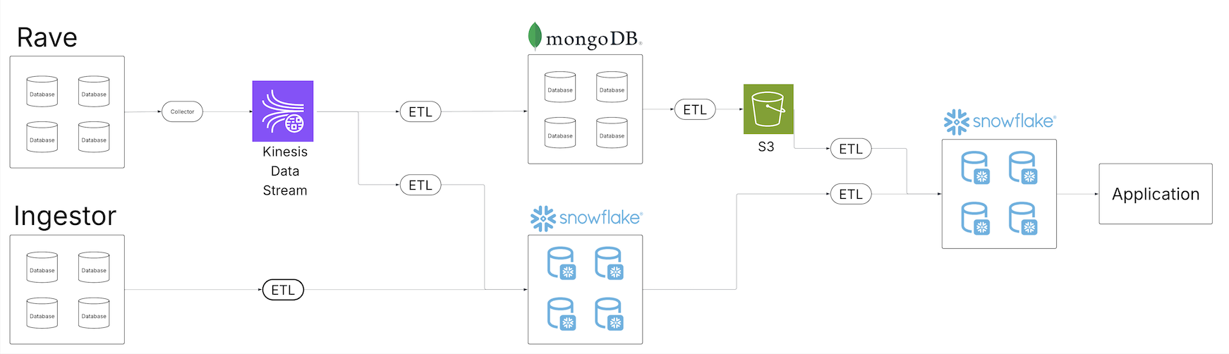
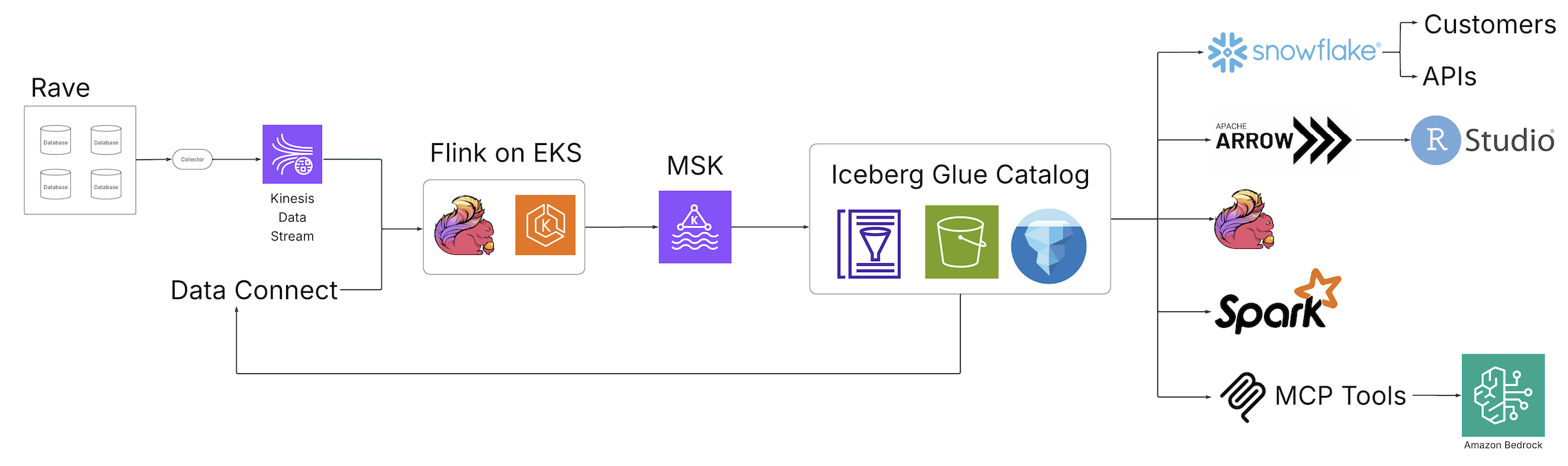
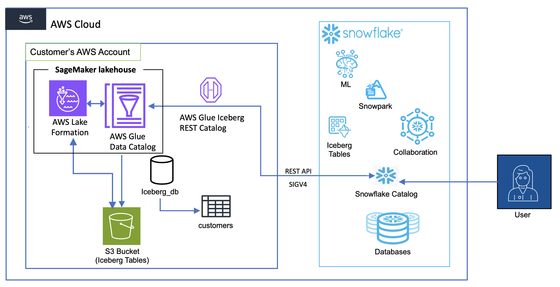
We run two versions of the same architecture: one where the tables are auto compacted, and another without compaction using in this case S3 Tables. By comparing both scenarios, this post demonstrates the efficiency, query performance, and cost benefits of auto compacted tables vs. non-compacted tables in a simulated Internet of Things (IoT) data pipeline. The following diagram illustrates the solution architecture.

Figure 1 – Solution architecture diagram
Compaction performance test
We simulated IoT data ingestion with over 20 billion events and used MERGE INTO for data deduplication across two time-based partitions, involving heavy partition reads and shuffling. After ingestion, we ran queries in Athena to compare performance between compacted and uncompacted tables using the Merge on Read (MoR) mode on both Avro and ORC formats. We use the following table configuration settings:
'write.delete.mode'='merge-on-read'
'write.update.mode'='merge-on-read'
'write.merge.mode'='merge-on-read'
'write.distribution.mode=hash'
We use 'write.distribution.mode=hash' to generate bigger files that will benefit the performance. Note that as we are generating quite large files already the differences between un-compacted and compacted tables are not going to that big, this will change significantly depending on your workload (for example, partitioning, input rate, batch size) and your chosen write distribution mode. For more details, please refer to the Writing Distribution Modes section in the Apache Iceberg documentation.
The following table shows metrics of the Athena query performance. Please refer to section “Query and Join data from these S3 Tables to build insights” for query details. All table sizes used to analyze the query performance are over 2 billion rows. These results are specific to this simulation exercise and the readers’ results may vary depending on their data size and queries they are running.
| Query |
Avro query time compaction |
Avro query time without compaction |
ORC query time without compaction |
ORC query time with compaction |
% improvement Avro |
% improvement ORC |
| Query 1 |
22.45 secs |
26.54 secs |
30.16 secs |
20.32 secs |
15.41% |
32.63% |
| Query 2 |
22.68 secs |
25.83 secs |
34.17 secs |
20.51 secs |
12.20% |
39.98% |
| Query 3 |
25.92 secs |
35.65 secs |
29.05 secs |
24.95 secs |
27.29% |
14.11% |
Prerequisites
To set up your own evaluation environment and test the feature, you need the following prerequisites.
AWS account with access to the following AWS services:
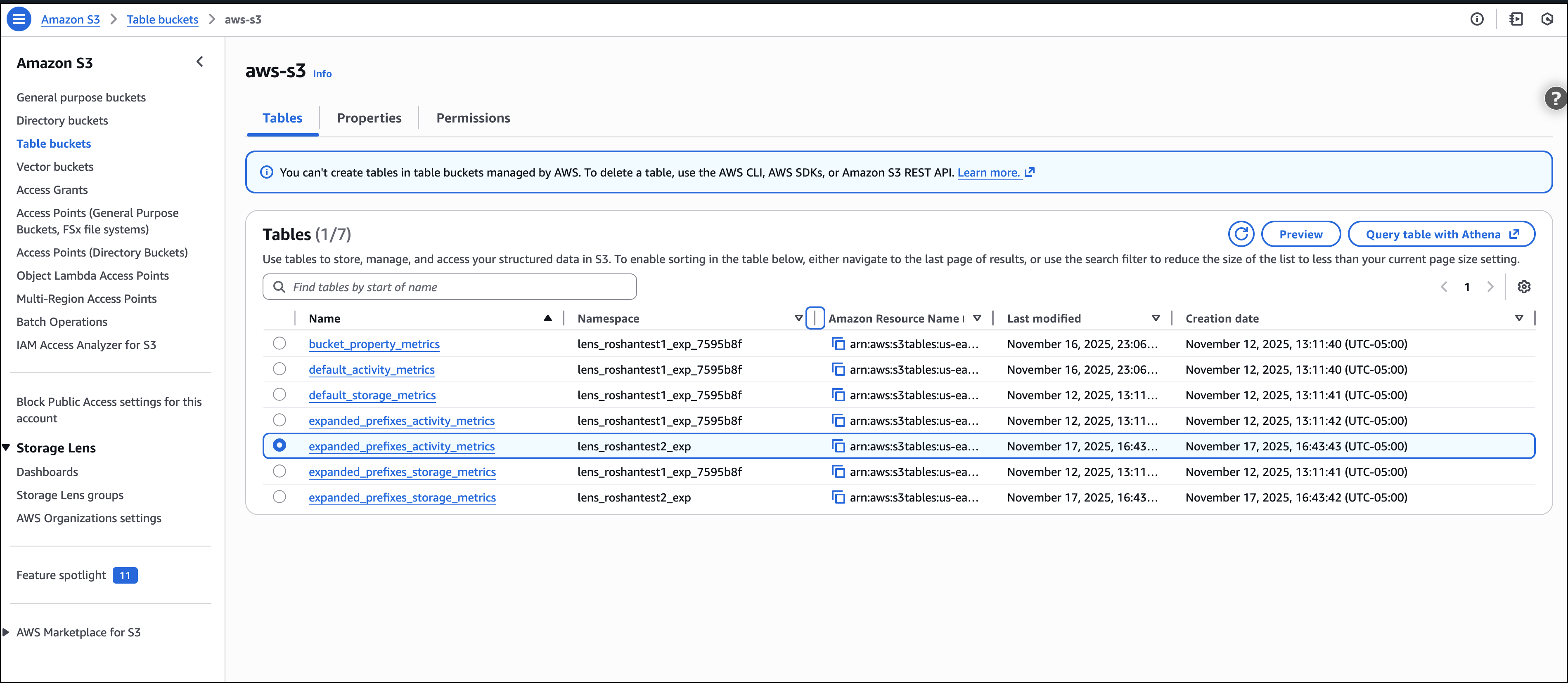
Create S3 table bucket and enable integration with AWS analytics services
Go to S3 console and enable table buckets feature.
Then choose the Create table bucket button, fill Table bucket name with any bucket name you prefer, select the Enable integration checkbox, then choose Create table bucket.
Set up Amazon S3 storage
Create an S3 bucket with the following structure:
s3bucket/
/jars
/employee.desc
/checkpointAvro
/checkpointAvroAuto
/checkpointORC
/checkpointORCAuto
Download the descriptor file employee.desc from the GitHub repo and put it into the S3 bucket you just created.
Download the application on the releases page
Get the packaged application S3Tables-Avro-orc-auto-compaction-benchmark-0.1 from the GitHub repo, then upload the JAR file to the “jars” directory on the S3 bucket. Checkpoint will be used for the Structured Streaming checkpointing mechanism. Because we use 4 streaming job runs, one for compacted and one for uncompacted data on each format, we also create a “checkpointAuto” folder for both.
Create an EMR Serverless application
Create an EMR Serverless application with the following settings (for instructions, see Getting started with Amazon EMR Serverless):
- Type: Spark
- Version: 7.20
- Architecture: x86_64
- Java Runtime: Java 17
- Metastore Integration: AWS Glue Data Catalog
- Logs: Enable Amazon CloudWatch Logs if desired (it’s recommended but not required for this blog)
Configure the network (VPC, subnets, and default security group) to allow the EMR Serverless application to reach the MSK cluster. Take note of the application-id to use later for launching the jobs.
Create an MSK cluster
Create an MSK cluster on the Amazon MSK console. For more details, see Get started using Amazon MSK. You need to use custom create with at least two brokers using 3.5.1, Apache Zookeeper mode version, and instance type kafka.m7g.xlarge. Do not use public access, instead choose two private subnets to deploy (one broker per subnet or Availability Zone, for a total of two brokers). For the security group, remember that the EMR cluster and the Amazon EC2 based producer will need to reach the cluster and act accordingly.
For security, use PLAINTEXT (in production, you should secure access to the cluster). Choose 200 GB as storage size for each broker and do not enable tiered storage. For network security groups, you can choose the default of the VPC.
For the MSK cluster configuration, use the following settings:
auto.create.topics.enable=true
default.replication.factor=2
min.insync.replicas=2
num.io.threads=8
num.network.threads=5
num.partitions=32
num.replica.fetchers=2
replica.lag.time.max.ms=30000
socket.receive.buffer.bytes=102400
socket.request.max.bytes=104857600
socket.send.buffer.bytes=102400
unclean.leader.election.enable=true
zookeeper.session.timeout.ms=18000
compression.type=zstd
log.retention.hours=2
log.retention.bytes=10073741824
Configure the data simulator
Log in to your EC2 instance. Because it’s running on a private subnet, you can use an instance endpoint to connect. To create one, see Connect to your instances using EC2 Instance Connect Endpoint. After you log in, issue the following commands:
sudo yum install java-17-amazon-corretto-devel
wget https://archive.apache.org/dist/kafka/3.5.1/kafka_2.12-3.5.1.tgz
tar xzvf kafka_2.12-3.5.1.tgz
Create Kafka topics
Create two Kafka topics—remember that you need to change the bootstrap server with the corresponding client information. You can get this data from the Amazon MSK console on the details page for your MSK cluster.
cd kafka_2.12-3.5.1/bin/

./kafka-topics.sh --topic protobuf-demo-topic-pure --bootstrap-server kafkaBoostrapString –create
Launching EMR Serverless Jobs for Iceberg Tables (Avro/ORC – Compacted & Non-Compacted)
Now it is time to launch EMR Serverless streaming jobs for four different Iceberg tables. Each job uses a different Spark Structured Streaming checkpoint and a specific Java class for ingestion logic.
Before launching the jobs, make sure:
- You have disabled auto-compaction in the S3 tables where necessary (see S3 Tables maintenance). In this case for
employee_Avro_uncompacted and employee_orc_uncompacted tables.
- Your EMR Serverless IAM role has permissions to read/write from S3Tables. Open AWS Lake formation console, then, you can follow these docs to give permissions to the EMR Serverless Role.
After launching each job launch the data simulator and let it finish. Then you can cancel the job run and launch the next one ( while launching the data simulator again).
Launch the data simulator
Download the JAR file to the EC2 instance and run the producer, note that will do this once.
aws s3 cp s3://s3bucket/jars/streaming-iceberg-ingest-1.0-SNAPSHOT.jar .
Now you can start the protocol buffer producers. Use the following commands:
java -cp streaming-iceberg-ingest-1.0-SNAPSHOT.jar
com.aws.emr.proto.kafka.producer.ProtoProducer kafkaBoostrapString
You should run this command for each of the tables ( job runs), run the command after the ingestion process has started.
Table 1: employee_orc_uncompacted
Checkpoint: checkpointORC
Java Class: SparkCustomIcebergIngestMoRS3BucketsORC
aws emr-serverless start-job-run \
  --application-id application-identifier \
  --name employee-orc-uncompacted-job \
  --execution-role-arn arn-of-emrserverless-role \
  --mode 'STREAMING' \
  --job-driver '{
    "sparkSubmit": {
      "entryPoint": "s3://s3bucket/jars/streaming-iceberg-ingest-1.0-SNAPSHOT.jar",
      "entryPointArguments": ["true", "s3://s3bucket/warehouse", "s3://s3bucket/Employee.desc", "s3://s3bucket/checkpointORC", "kafkaBootstrapString", "true"],
      "sparkSubmitParameters": "--class com.aws.emr.spark.iot.SparkCustomIcebergIngestMoRS3BucketsORC --conf spark.executor.cores=16 --conf spark.executor.memory=64g --conf spark.driver.cores=4 --conf spark.driver.memory=16g --conf spark.dynamicAllocation.minExecutors=3 --conf spark.dynamicAllocation.maxExecutors=5 --conf spark.sql.catalog.glue_catalog.http-client.apache.max-connections=3000 --conf spark.emr-serverless.executor.disk.type=shuffle_optimized --conf spark.emr-serverless.executor.disk=1000G --conf spark.jars /usr/share/aws/iceberg/lib/iceberg-spark3-runtime.jar --files s3://s3bucket/Employee.desc --packages org.apache.spark:spark-sql-kafka-0-10_2.12:3.5.1"
    }
  }'
Table 2: employee_avro_uncompacted
Checkpoint: checkpointAvro
Java Class: SparkCustomIcebergIngestMoRS3BucketsAvro
aws emr-serverless start-job-run \
  --application-id application-identifier \
  --name employee-Avro-uncompacted-job \
  --execution-role-arn arn-of-emrserverless-role \
  --mode 'STREAMING' \
  --job-driver '{
    "sparkSubmit": {
      "entryPoint": "s3://s3bucket/jars/streaming-iceberg-ingest-1.0-SNAPSHOT.jar",
      "entryPointArguments": ["true", "s3://s3bucket/warehouse", "s3://s3bucket/Employee.desc", "s3://s3bucket/checkpointAvro", "kafkaBootstrapString", "true"],
      "sparkSubmitParameters": "--class com.aws.emr.spark.iot.SparkCustomIcebergIngestMoRS3BucketsAvro --conf spark.executor.cores=16 --conf spark.executor.memory=64g --conf spark.driver.cores=4 --conf spark.driver.memory=16g --conf spark.dynamicAllocation.minExecutors=3 --conf spark.dynamicAllocation.maxExecutors=5 --conf spark.sql.catalog.glue_catalog.http-client.apache.max-connections=3000 --conf spark.emr-serverless.executor.disk.type=shuffle_optimized --conf spark.emr-serverless.executor.disk=1000G --conf spark.jars  /usr/share/aws/iceberg/lib/iceberg-spark3-runtime.jar --files s3://s3bucket/Employee.desc --packages org.apache.spark:spark-sql-kafka-0-10_2.12:3.5.1"
    }
  }'
Table 3: employee_orc (Auto-Compacted)
Checkpoint: checkpointORCAuto
Java Class: SparkCustomIcebergIngestMoRS3BucketsAutoORC
aws emr-serverless start-job-run \
  --application-id application-identifier \
  --name employee-orc-auto-job \
  --execution-role-arn arn-of-emrserverless-role \
  --mode 'STREAMING' \
  --job-driver '{
    "sparkSubmit": {
      "entryPoint": "s3://s3bucket/jars/streaming-iceberg-ingest-1.0-SNAPSHOT.jar",
      "entryPointArguments": ["true", "s3://s3bucket/warehouse", "s3://s3bucket/Employee.desc", "s3://s3bucket/checkpointORCAuto", "kafkaBootstrapString", "true"],
      "sparkSubmitParameters": "--class com.aws.emr.spark.iot.SparkCustomIcebergIngestMoRS3BucketsAutoORC --conf spark.executor.cores=16 --conf spark.executor.memory=64g --conf spark.driver.cores=4 --conf spark.driver.memory=16g --conf spark.dynamicAllocation.minExecutors=3 --conf spark.dynamicAllocation.maxExecutors=5 --conf spark.sql.catalog.glue_catalog.http-client.apache.max-connections=3000 --conf spark.emr-serverless.executor.disk.type=shuffle_optimized --conf spark.emr-serverless.executor.disk=1000G --conf spark.jars /usr/share/aws/iceberg/lib/iceberg-spark3-runtime.jar --files s3://s3bucket/Employee.desc --packages org.apache.spark:spark-sql-kafka-0-10_2.12:3.5.1"
    }
  }'
Table 4: employee_avro (Auto-Compacted)
Checkpoint: checkpointAvroAuto
Java Class: SparkCustomIcebergIngestMoRS3BucketsAutoAvro
aws emr-serverless start-job-run \
  --application-id application-identifier \
  --name employee-Avro-auto-job \
  --execution-role-arn arn-of-emrserverless-role \
  --mode 'STREAMING' \
  --job-driver '{
    "sparkSubmit": {
      "entryPoint": "s3://s3bucket/jars/streaming-iceberg-ingest-1.0-SNAPSHOT.jar",
      "entryPointArguments": ["true", "s3://s3bucket/warehouse", "s3://s3bucket/Employee.desc", "s3://s3bucket/checkpointAvroAuto", "kafkaBootstrapString", "true"],
      "sparkSubmitParameters": "--class com.aws.emr.spark.iot.SparkCustomIcebergIngestMoRS3BucketsAutoAvro --conf spark.executor.cores=16 --conf spark.executor.memory=64g --conf spark.driver.cores=4 --conf spark.driver.memory=16g --conf spark.dynamicAllocation.minExecutors=3 --conf spark.dynamicAllocation.maxExecutors=5 --conf spark.sql.catalog.glue_catalog.http-client.apache.max-connections=3000 --conf spark.emr-serverless.executor.disk.type=shuffle_optimized --conf spark.emr-serverless.executor.disk=1000G --conf spark.jars /usr/share/aws/iceberg/lib/iceberg-spark3-runtime.jar --files s3://s3bucket/Employee.desc --packages org.apache.spark:spark-sql-kafka-0-10_2.12:3.5.1"
    }
  }'
Query and Join data from these S3 Tables to build insights
You can go to Athena console and then run the queries. Please ensure that Lake Formation permissions are applied on the catalog database and tables for your IAM Console role. For more details, please refer to docs on the Grant Lake Formation permissions on your table.
To benchmark these queries in Athena, you can run each query multiple times—typically five runs per query—to obtain a reliable performance estimate. In the Athena console, simply execute the same query repeatedly and record the execution time for each run, which is displayed in the query history. Once you have five execution times, calculate the average to get a representative benchmark value. This approach helps account for variations in performance due to background load, providing more consistent and meaningful results.
Query 1
SELECT role, team, avg(age) AS average_age
FROM bigdata."employee_orc"
GROUP BY role, team
ORDER BY average_age DESC
Query 2
SELECT team, name, min(age) as youngest_age
FROM "bigdata"."employee_Avro"
GROUP BY team, name
ORDER BY youngest_age ASC
Query 3
SELECT name, age, start_date, role, team
FROM bigdata."employee_Avro"
WHERE CAST(start_date as DATE) > CAST('2023-01-02' as DATE) and age > 40
ORDER BY start_date DESC
limit 100
Conclusion
AWS has expanded support for Iceberg table optimization to include all Iceberg supported file formats: Parquet, Avro, and ORC. This comprehensive compaction capability is now available for both Amazon S3 Tables and Iceberg tables in general purpose S3 buckets using the lakehouse architecture in SageMaker with Glue Data Catalog optimization. S3 Tables deliver a fully managed experience through continual optimization, automatically maintaining your tables by handling compaction, snapshot retention, and unreferenced file removal. These automated maintenance features significantly improve query performance and reduce query engine costs. Compaction support for Avro and ORC formats is now available in all AWS Regions where S3 Tables or optimization with the AWS Glue Data Catalog are available. To learn more about S3 Tables compaction, see the S3 Tables maintenance documentation. For general purpose bucket optimization, see the Glue Data Catalog optimization documentation.
Special thanks to everyone who contributed to this launch: Matthieu Dufour, Srishti Bhargava, Stylianos Herodotou, Kannan Ratnasingham, Shyam Rathi, David Lee.
About the authors
 Angel Conde Manjon is a Sr. EMEA Data & AI PSA, based in Madrid. He has previously worked on research related to Data Analytics and Artificial Intelligence in diverse European research projects. In his current role, Angel helps partners develop businesses centered on Data and AI.
 Diego Colombatto is a Principal Partner Solutions Architect at AWS. He brings more than 15 years of experience in designing and delivering Digital Transformation projects for enterprises. At AWS, Diego works with partners and customers advising how to leverage AWS technologies to translate business needs into solutions. Solution architectures, algorithmic trading and cooking are some of his passions and he’s always open to start a conversation on these topics.
 Sandeep Adwankar is a Senior Technical Product Manager at AWS. Based in the California Bay Area, he works with customers around the globe to translate business and technical requirements into products that enable customers to improve how they manage, secure, and access data.


 Sohaib Katariwala is a Senior Specialist Solutions Architect at AWS focused on Amazon OpenSearch Service based out of Chicago, IL. His interests are in all things data and analytics. More specifically he loves to help customers use AI in their data strategy to solve modern day challenges.
 Mark Twomey is a Senior Solutions Architect at AWS focused on storage and data management. He enjoys working with customers to put their data in the right place, at the right time, for the right cost. Living in Ireland, Mark enjoys walking in the countryside, watching movies, and reading books.
 Sorabh Hamirwasia is a senior software engineer at AWS working on the OpenSearch Project. His primary interest include building cost optimized and performant distributed systems.
 Pallavi Priyadarshini is a Senior Engineering Manager at Amazon OpenSearch Service leading the development of high-performing and scalable technologies for search, security, releases, and dashboards.
 Bobby Mohammed is a Principal Product Manager at AWS leading the Search, GenAI, and Agentic AI product initiatives. Previously, he worked on products across the full lifecycle of machine learning, including data, analytics, and ML features on SageMaker platform, deep learning training and inference products at Intel.
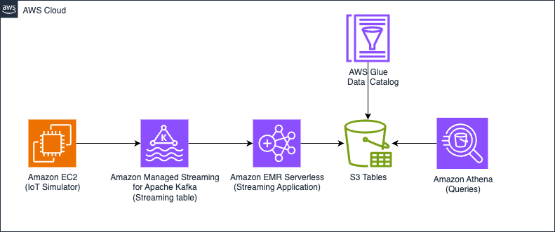
 Angel Conde Manjon is a Sr. EMEA Data & AI PSA, based in Madrid. He has previously worked on research related to Data Analytics and Artificial Intelligence in diverse European research projects. In his current role, Angel helps partners develop businesses centered on Data and AI.
 Diego Colombatto is a Principal Partner Solutions Architect at AWS. He brings more than 15 years of experience in designing and delivering Digital Transformation projects for enterprises. At AWS, Diego works with partners and customers advising how to leverage AWS technologies to translate business needs into solutions. Solution architectures, algorithmic trading and cooking are some of his passions and he’s always open to start a conversation on these topics.
 Sandeep Adwankar is a Senior Technical Product Manager at AWS. Based in the California Bay Area, he works with customers around the globe to translate business and technical requirements into products that enable customers to improve how they manage, secure, and access data.


 Amit Maindola is a Senior Data Architect focused on data engineering, analytics, and AI/ML at Amazon Web Services. He helps customers in their digital transformation journey and enables them to build highly scalable, robust, and secure cloud-based analytical solutions on AWS to gain timely insights and make critical business decisions.
 Srinivas Kandi is a Senior Architect at Stifel focusing on delivering the next generation of cloud data platform on AWS. Prior to joining Stifel, Srini was a delivery specialist in cloud data analytics at AWS helping several customers in their transformational journey into AWS cloud. In his free time, Srini likes to explore cooking, travel and learn new trends and innovations in AI and cloud computing.
 Hossein Johari is a seasoned data and analytics leader with over 25 years of experience architecting enterprise-scale platforms. As Lead and Senior Architect at Stifel Financial Corp. in St. Louis, Missouri, he spearheads initiatives in Data Platforms and Strategic Solutions, driving the design and implementation of innovative frameworks that support enterprise-wide analytics, strategic decision-making, and digital transformation. Known for aligning technical vision with business objectives, he works closely with cross-functional teams to deliver scalable, forward-looking solutions that advance organizational agility and performance.
 Ahmad Rawashdeh is a Senior Architect at Stifel Financial. He supports Stifel and its clients in designing, implementing, and building scalable and reliable data architectures on Amazon Web Services (AWS), with a strong focus on data lake strategies, database services, and efficient data ingestion and transformation pipelines.
 Lei Meng is a data architect at Stifel. His focus is working in designing and implementing scalable and secure data solutions on the AWS and helping Stifel’s cloud migration from on-premises systems.