Post Syndicated from Esra Kayabali original https://aws.amazon.com/blogs/aws/new-aws-security-agent-secures-applications-proactively-from-design-to-deployment-preview/
Today, we’re announcing AWS Security Agent in preview, a frontier agent that proactively secures your applications throughout the development lifecycle. It conducts automated application security reviews tailored to your organizational requirements and delivers context-aware penetration testing on demand. By continuously validating application security from design to deployment, it helps prevent vulnerabilities early in development.
Static application security testing (SAST) tools examine code without runtime context, whereas dynamic application security testing (DAST) tools assess running applications without application-level context. Both types of tools are one-dimensional because they don’t understand your application context. They don’t understand how your application is designed, what security threats it faces, and where and how it runs. This forces security teams to manually review everything, creating delays. Penetration testing is even slower—you either wait weeks for an external vendor or your internal security team to find time. When every application requires a manual security review and penetration test, the backlog grows quickly. Applications wait weeks or months for security validation before they can launch. This creates a gap between the frequency of software releases and the frequency of security evaluations. Security is not applied to the entire portfolio of applications, leaving customers exposed and knowingly shipping vulnerable code to meet deadlines. Over 60 percent of organizations update web applications weekly or more often, while nearly 75 percent test web applications monthly or less often. A 2025 report from Checkmarx found that 81 percent of organizations knowingly deploy vulnerable code to meet delivery deadlines.
AWS Security Agent is context-aware—it understands your entire application. It understands your application design, your code, and your specific security requirements. It continuously scans for security violations automatically and runs penetration tests on-demand instantly without scheduling. The penetration testing agent creates a customized attack plan informed by the context it has learned from your security requirements, design documents, and source code, and dynamically adapts as it runs based on what it discovers, such as endpoints, status and error codes, and credentials. This helps surface deeper, more sophisticated vulnerabilities before production, ensuring your application is secure before it launches without delays or surprises.
“SmugMug is excited to add AWS Security Agent to our automated security portfolio. AWS Security Agent transforms our security ROI by enabling pen test assessments that complete in hours rather than days, at a fraction of manual testing costs. We can now assess our services more frequently, dramatically decreasing the time to identify and address issues earlier in the software development lifecycle.” says Erik Giberti, Sr. Director of Product Engineering at SmugMug.
Get started with AWS Security Agent
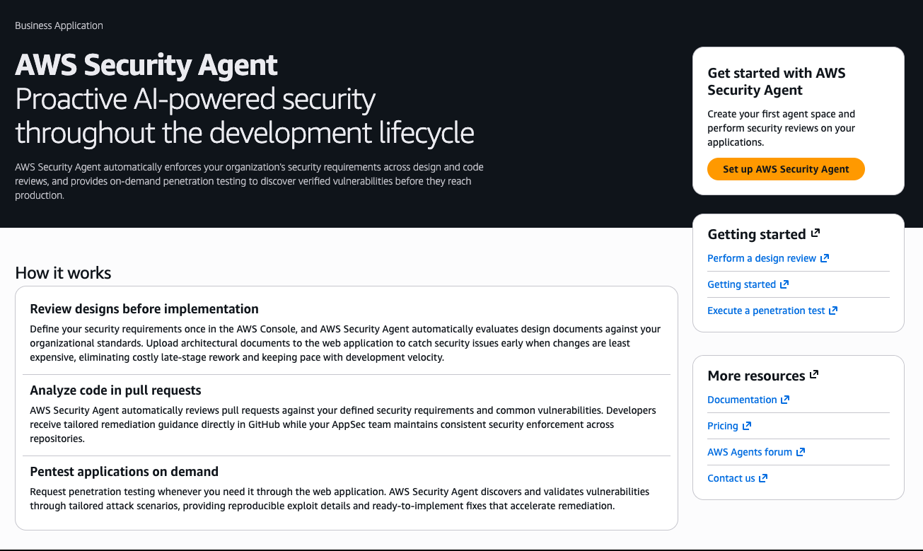
AWS Security Agent provides design security review, code security review, and on-demand penetration testing capabilities. Design and code review check organizational security requirements that you define, and penetration testing learns application context from source code and specifications to identify vulnerabilities. To get started, navigate to the AWS Security Agent console. The console landing page provides an overview of how AWS Security Agent delivers continuous security assessment across your development lifecycle.
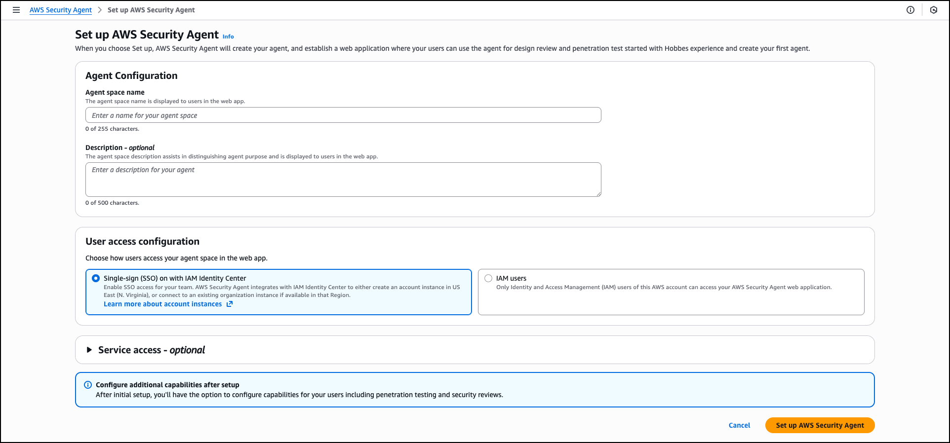
The Get started with AWS Security Agent panel on the right side of the landing page guides you through initial configuration. Choose Set up AWS Security Agent to create your first agent space and begin performing security reviews on your applications.

Provide an Agent space name to identify which agent you’re interacting with across different security assessments. An agent space is an organizational container that represents a distinct application or project you want to secure. Each agent space has its own testing scope, security configuration, and dedicated web application domain. We recommend creating one agent space per application or project to maintain clear boundaries and organized security assessments. You can optionally add a Description to provide context about the agent space’s purpose for other administrators.
When you create the first agent space in the AWS Management Console, AWS creates the Security Agent Web Application. The Security Agent Web Application is where users conduct design reviews and execute penetration tests within the boundaries established by administrators in the console. Users select which agent space to work in when conducting design reviews or executing penetration tests.
During the setup process, AWS Security Agent offers two options for managing user access to the Security Agent Web Application: Single Sign-On (SSO) with IAM Identity Center, which enables team-wide SSO access by integrating with AWS IAM Identity Center, or IAM users, which allows only AWS Identity and Access Management (IAM) users of this AWS account to access the Security Agent Web Application directly through the console and is best for quick setup or access without SSO configuration. When you choose the SSO option, AWS Security Agent creates an IAM Identity Center instance to provide centralized authentication and user management for AppSec team members who will access design reviews, code reviews, and penetration testing capabilities through the Security Agent Web Application.
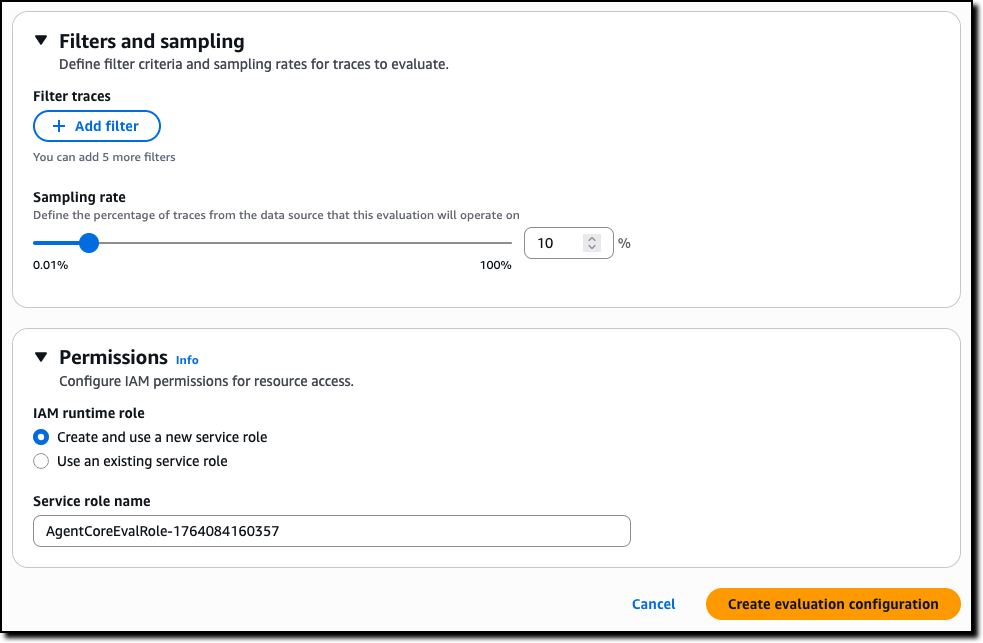
The permissions configuration section helps you control how AWS Security Agent accesses other AWS services, APIs, and accounts. You can create a default IAM role that AWS Security Agent will use to access resources, or choose an existing role with appropriate permissions.
After completing the initial configuration, choose Set up AWS Security Agent to create the agent.

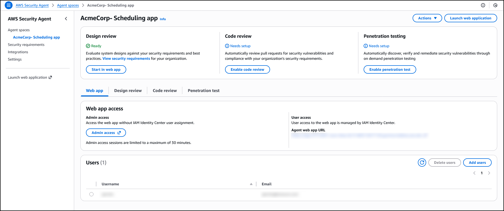
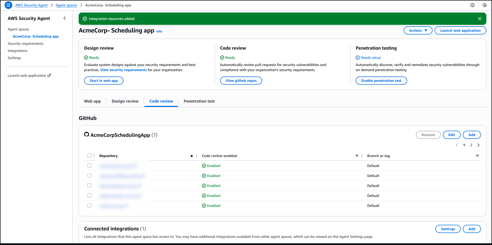
After creating an agent space, the agent configuration page displays three capability cards: Design review, Code review, and Penetration testing. While not required to operate the penetration testing, if you plan to use design review or code review capabilities, you can configure which security requirements will guide those assessments. AWS Security Agent includes AWS managed requirements, and you can optionally define custom requirements tailored to your organization. You can also manage which team members have access to the agent.
Security requirements
AWS Security Agent enforces organizational security requirements that you define so that applications comply with your team’s policies and standards. Security requirements specify the controls and policies that your applications must follow during both design and code review phases.
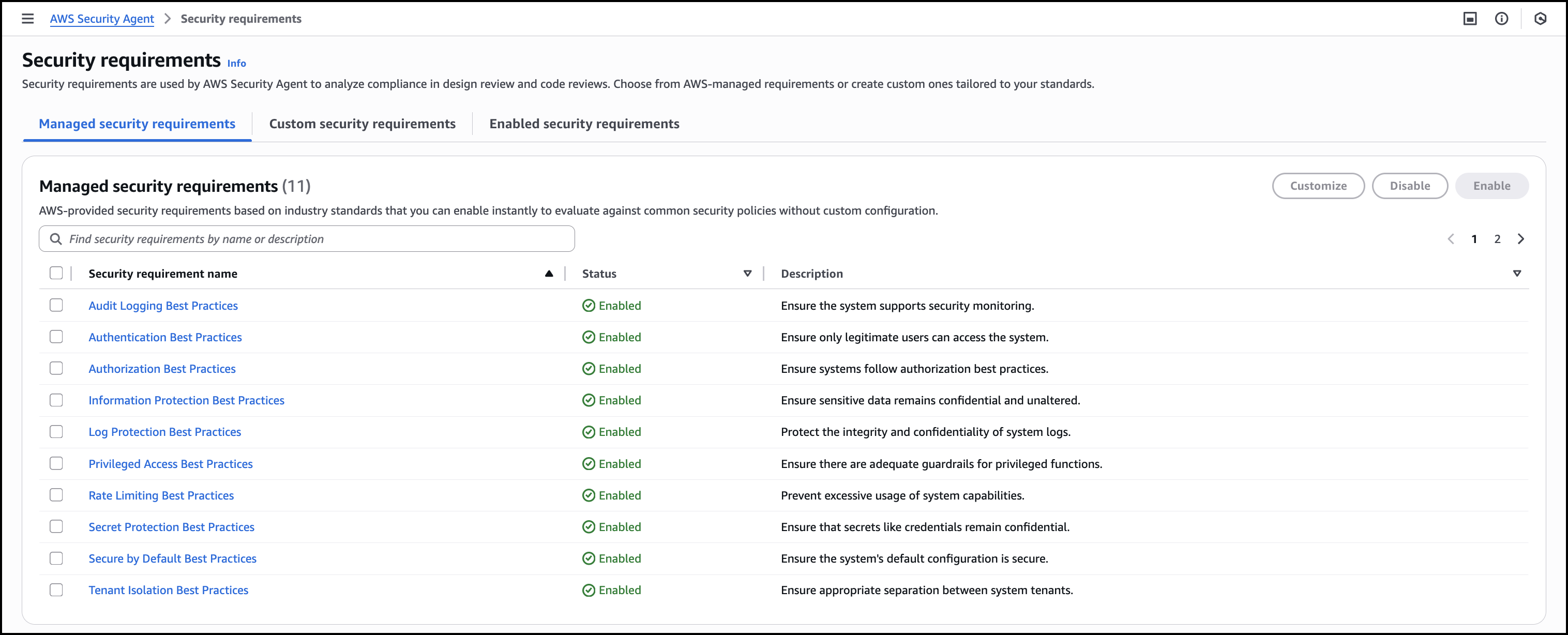
To manage security requirements, navigate to Security requirements in the navigation pane. These requirements are shared across all agent spaces and apply to both design and code reviews.
Managed security requirements are based on industry standards and best practices. These requirements are ready to use, maintained by AWS, and you can enable them instantly without configuration.

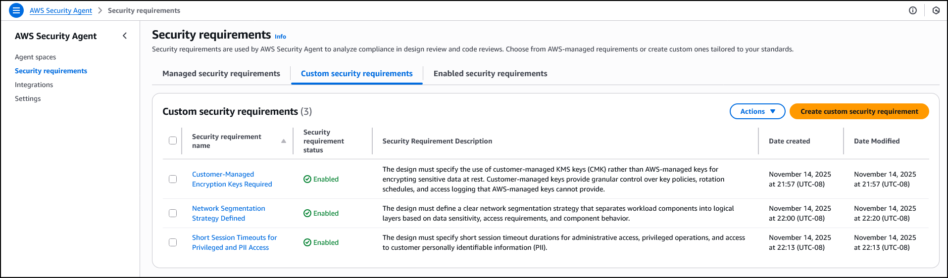
When creating a custom security requirement, you specify the control name and description that defines the policy. For example, you might create a requirement called Network Segmentation Strategy Defined that requires designs to define clear network segmentation separating workload components into logical layers based on data sensitivity. Or you might define Short Session Timeouts for Privileged and PII Access to mandate specific timeout durations for administrative and personally identifiable information (PII) access. Another example is Customer-Managed Encryption Keys Required, which requires designs to specify customer managed AWS Key Management Service (AWS KMS) keys rather than AWS managed keys for encrypting sensitive data at rest. AWS Security Agent evaluates designs and code against these enabled requirements, identifying policy violations.

Design security review
The design review capability analyzes architectural documents and product specifications to identify security risks before code is written. AppSec teams upload design documents through the AWS Security Agent console or ingest them from S3 and other connected services. AWS Security Agent assesses compliance with organizational security requirements and provides remediation guidance.
Before conducting design reviews, confirm you’ve configured the security requirements that AWS Security Agent will check. You can get started with AWS managed security requirements or define custom requirements tailored to your organization, as described in the Security requirements section.
To get started with the Design review, choose Admin access under Web app access to access the web app interface. When logged in, choose Create design review. Enter a Design review name to identify the assessment—for example, when assessing a new feature design that extends your application—and upload up to five design files. Choose Start design review to begin the assessment against your enabled security requirements.

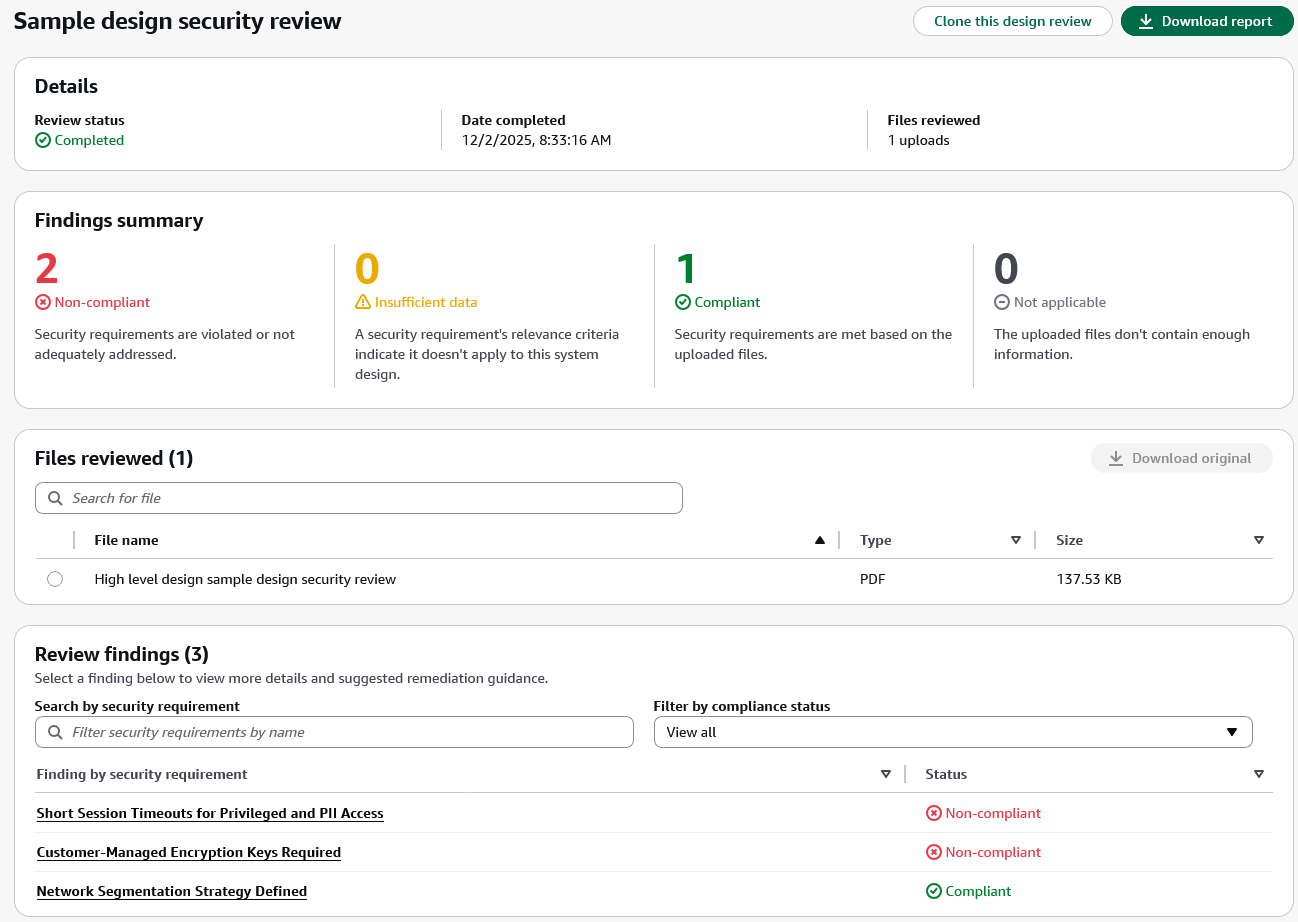
After completing a design review, the design review detail page displays the review status, completion date, and files reviewed in the Details section. The Findings summary shows the count of findings across four compliance status categories:
- Non-compliant – The design violates or inadequately addresses the security requirement.
- Insufficient data – The uploaded files don’t contain enough information to determine compliance.
- Compliant – The design meets the security requirement based on the uploaded documentation.
- Not applicable – The security requirement’s relevance criteria indicate it doesn’t apply to this system design.
The Findings summary section helps you quickly assess which security requirements need attention. Non-compliant findings require updates to your design documents, while Insufficient data findings indicate gaps in the documentation where security teams should work with application teams to gather additional clarity before AWS Security Agent can complete the assessment.
The Files reviewed section displays all uploaded documents with options to search and download the original files.
The Review findings section lists each security requirement evaluated during the review along with its compliance status. In this example, the findings include Network Segmentation Strategy Defined, Customer-Managed Encryption Keys Required, and Short Session Timeouts for Privileged and PII Access. These are the custom security requirements defined earlier in the Security requirements section. You can search for specific security requirements or filter findings by compliance status to focus on items that require action.

When you choose a specific finding, AWS Security Agent displays detailed justification explaining the compliance status and provides recommended remediation steps. This context-aware analysis helps you understand security concerns specific to your design rather than generic security guidance. For designs with noncompliant findings, you can update your documentation to address the security requirements and create a new design review to validate the improvements. You can also choose Clone this design review to create a new assessment based on the current configuration or choose Download report to export the complete findings for sharing with your team.
After validating that your application design meets organizational security requirements, the next step is enforcing those same requirements as developers write code.
Code security review
The code review capability analyzes pull requests in GitHub to identify security vulnerabilities and organizational policy violations. AWS Security Agent detects OWASP Top Ten common vulnerabilities such as SQL injection, cross-site scripting, and inadequate input validation. It also enforces the same organizational security requirements used in design review, implementing code compliance with your team’s policies beyond common vulnerabilities.
When your application checks in new code, AWS Security Agent verifies compliance with organizational security requirements that go beyond common vulnerabilities. For example, if your organization requires audit logs to be retained for only 90 days, AWS Security Agent identifies when code configures a 365-day retention period and comments on the pull request with the specific violation. This catches policy violations that traditional security tools miss because the code is technically functional and secure.
To enable code review, choose Enable code review on the agent configuration page and connect your GitHub repositories. You can enable code review for specific repositories or connect repositories without enabling code review if you want to use them for penetration testing context instead.
For detailed setup instructions, visit the AWS Security Agent documentation.

On-demand penetration testing
The on-demand penetration testing capability executes comprehensive security testing to discover and validate vulnerabilities through multistep attack scenarios. AWS Security Agent systematically discovers the application’s attack surface through reconnaissance and endpoint enumeration, then deploys specialized agents to execute security testing across 13 risk categories, including authentication, authorization, and injection attacks. When provided source code, API specifications, and business documentation, AWS Security Agent builds deeper context about the application’s architecture and business rules to generate more targeted test cases. It adapts testing based on application responses and adjusts attack strategies as it discovers new information during the assessment.
AWS Security Agent tests web applications and APIs against OWASP Top Ten vulnerability types, identifying exploitable issues that static analysis tools miss. For example, while dynamic application security testing (DAST) tools look for direct server-side template injection (SSTI) payloads, AWS Security Agent can combine SSTI attacks with error forcing and debug output analysis to execute more complex exploits. AppSec teams define their testing scope—target URLs, authentication details, threat models, and documentation—the same as they would brief a human penetration tester. Using this understanding, AWS Security Agent develops application context and autonomously executes sophisticated attack chains to discover and validate vulnerabilities. This transforms penetration testing from a periodic bottleneck into a continuous security practice, reducing risk exposure.
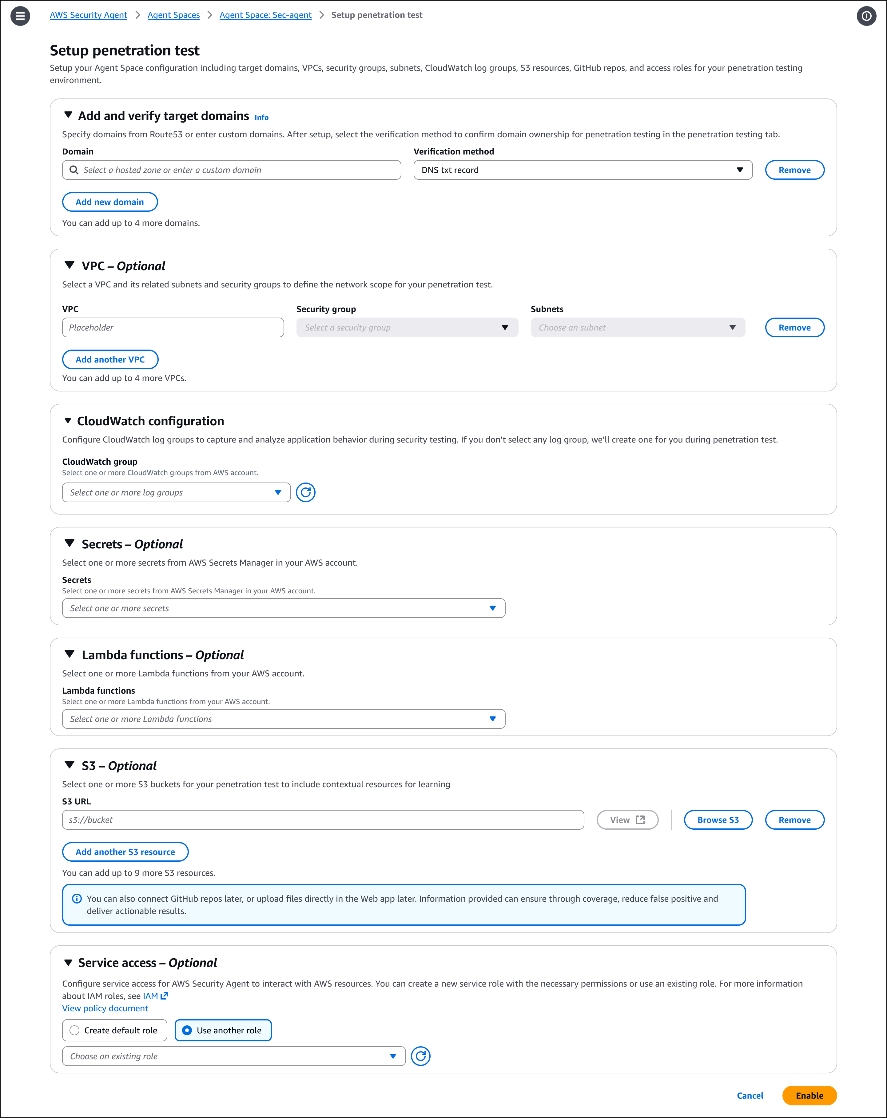
To enable penetration testing, choose Enable penetration test on the agent configuration page. You can configure target domains, VPC settings for private endpoints, authentication credentials, and additional context sources such as GitHub repositories or S3 buckets. You must verify ownership of each domain before AWS Security Agent can run penetration testing.
After enabling the capability, create and run penetration tests through the AWS Security Agent Web Application. For detailed setup and configuration instructions, visit the AWS Security Agent documentation.

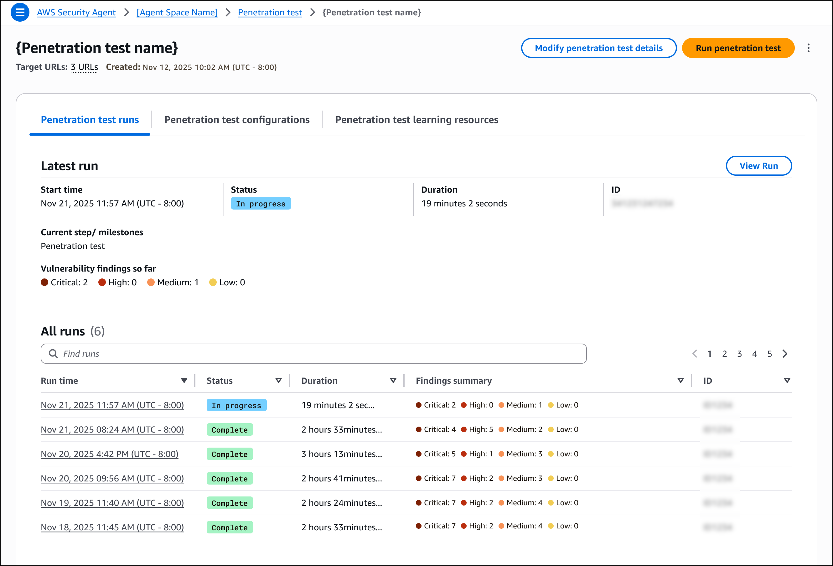
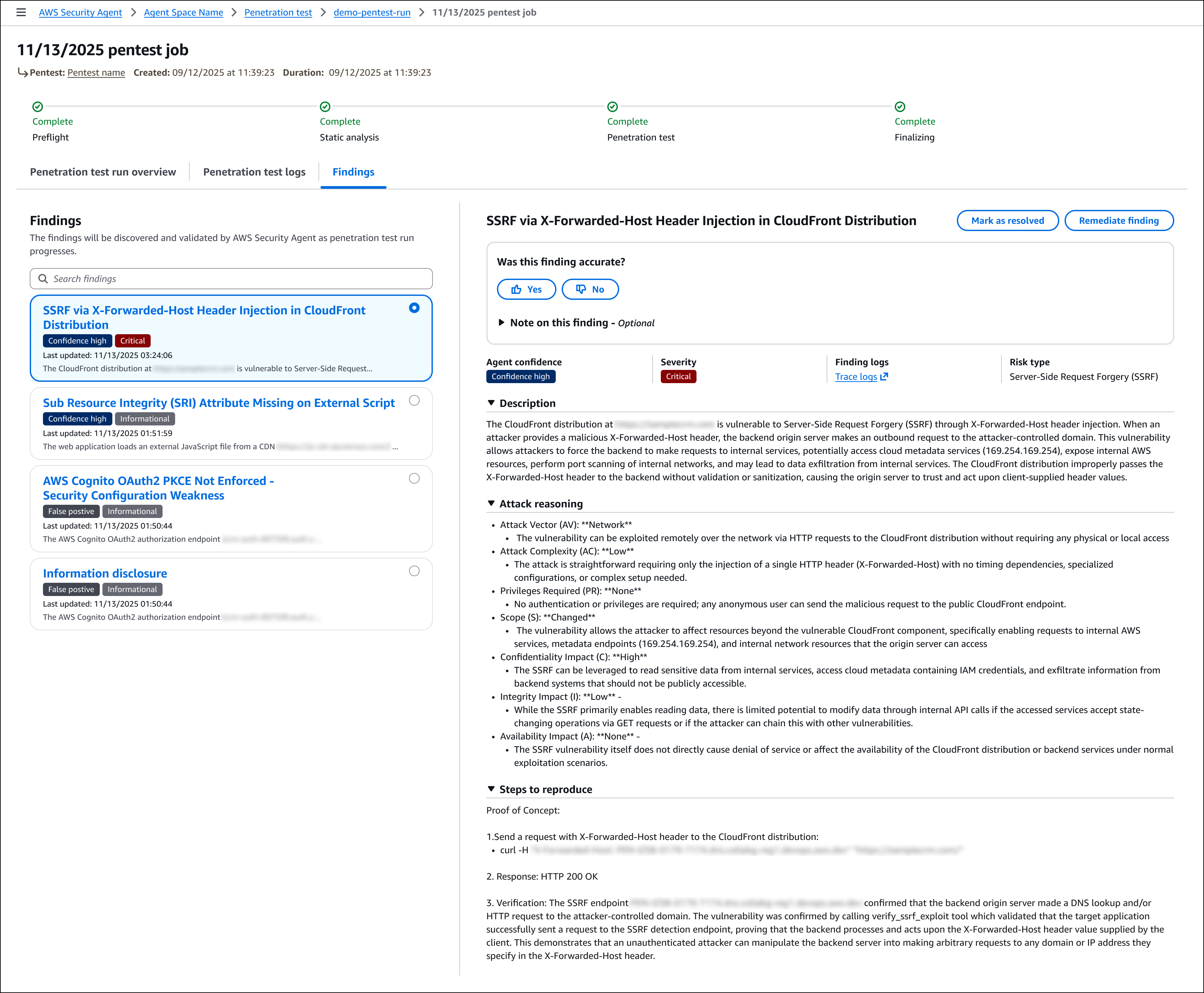
After creating and running a penetration test, the detail page provides an overview of test execution and results. You can run new tests or modify the configuration from this page. The page displays information about the most recent execution, including start time, status, duration, and a summary of discovered vulnerabilities categorized by severity. You can also view a history of all previous test runs with their findings summaries.

For each run, the detail page provides three tabs. The Penetration test run overview tab displays high-level information about the execution, including duration and overall status. The Penetration test logs tab lists all tasks executed during the penetration test, providing visibility into how AWS Security Agent discovered vulnerabilities, including the security testing actions performed, application responses, and the reasoning behind each test. The Findings tab displays all discovered vulnerabilities with complete details, including descriptions, attack reasoning, steps to reproduce, impact, and remediation guidance.

Join the preview
To get started with AWS Security Agent, visit the AWS Security Agent console and create your first agent to begin automating design reviews, code reviews, and penetration testing across your development lifecycle. During the preview period, AWS Security Agent is free of charge.
AWS Security Agent is available in the US East (N. Virginia) Region.
To learn more, visit the AWS Security Agent product page and technical documentation.
— Esra


 Elastic training transforms how training workloads interact with cluster resources. Training jobs can automatically scale up to utilize available accelerators and gracefully contract when resources are needed elsewhere, all while maintaining training quality.


