Tag Archives: launch

Announcing AWS Well-Architected Agent, an AI-powered intelligence to optimize your cloud environment (preview)

Post Syndicated from Channy Yun (윤석찬) original https://aws.amazon.com/blogs/aws/announcing-aws-well-architected-agent-an-ai-powered-intelligence-to-optimize-your-cloud-environment-preview/

Today, we’re announcing the public preview of AWS Well-Architected Agent, an AI-powered service that analyzes your AWS environment to deliver targeted, contextual recommendations for improving your applications’ cost, security, performance, and resilience. The AWS Well-Architected Agent analyzes your infrastructure, understands unique business goals, and delivers contextual recommendations with ready-to-implement fixes. It delivers context-aware optimization without relying on manual audits or generic checklists.

The agent evaluates your environment as an experienced cloud architect would. It automatically correlates utilization metrics, resource configurations, and application topology, and analyzes against Well-Architected best practices across 65+ AWS services. It generates recommendations aligned to your declared business goals, delivers implementation packages with every finding, and surfaces cross-pillar trade-offs making it simpler to remediate the findings.

Here are the three main features of this service:

  • Goal-aligned intelligence: AWS Well-Architected Agent replaces flat, undifferentiated findings with context-aware, prioritized recommendations. You declare your business objectives and share your application context. The agent automatically generates and prioritizes recommendations by impact and effort against those goals.
  • Three-level recommendations: AWS Well-Architected Agent provides individual resource findings with specific dollar impact (where applicable) and step-by-step remediation, consolidated findings across multiple resources scoped to your application, and broad architectural patterns and designs with Infrastructure as Code (IaC) code changes needed to align with Well-Architected best practices.
  • Optionality in remediation: You can choose your path on how you want to remediate with a complete implementation steps tailored to your environment: the console walk-throughs, updated IaC changes for architecture-level recommendations, and AWS Command Line Interface (AWS CLI) commands.

AWS Well-Architected Agent in action

To get started, create an agent profile to define the scope of what Well-Architected Agent can access and provide recommendations on, complete the IAM role setup to access resources, conduct architecture review, and remediate recommendations.

Create an agent profile

In the AWS Well-Architected console, choose Get started with Well-Architected Agent. You can define an agent profile that specifies which AWS accounts and applications to monitor, which optimization pillars to focus on, and the permissions required.
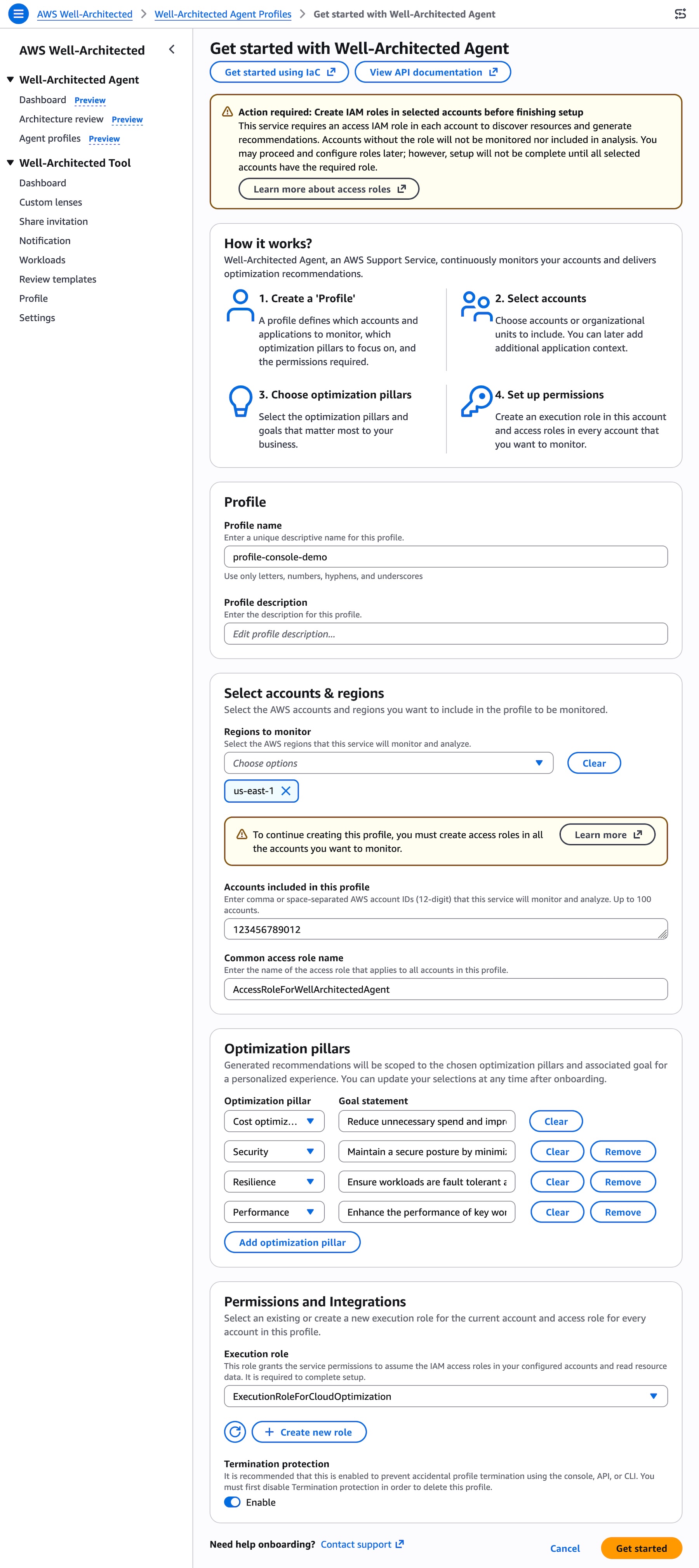
You can choose AWS accounts or AWS Regions to monitor and optimization pillars that matter most to your business. You can also set goals for each pillar: cost optimization, performance, resilience, and security.

To give access to the agent for your AWS environment, provision customer-managed IAM roles the agent uses to read resource configurations, utilization metrics, and application topology. To learn more, visit the IAM prerequisite for AWS Well-Architected Agent.

When you choose Get Started, the agent creates your agent profile. Resource and application recommendations will be generated within 24 hours after profile creation.
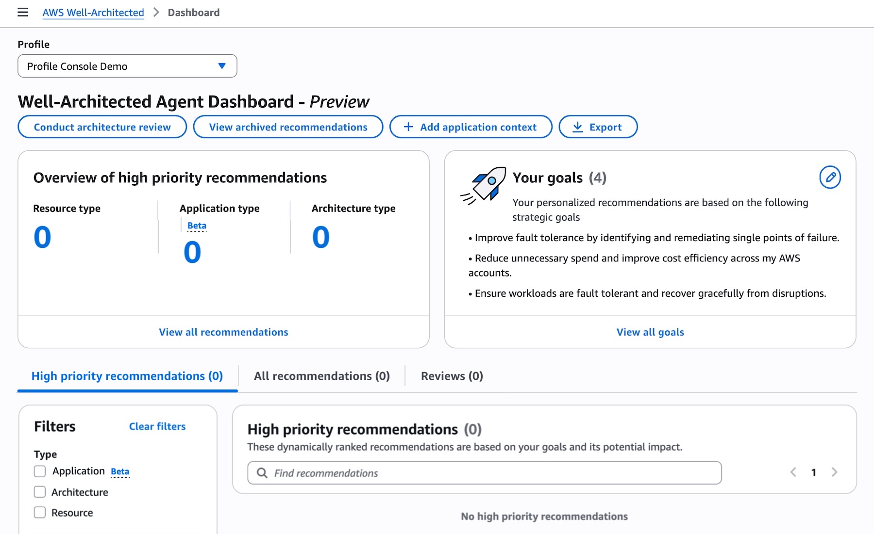
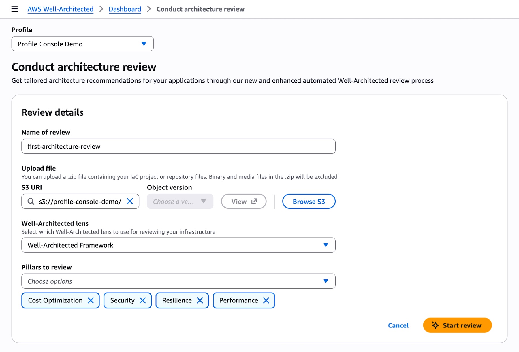
You can conduct an architecture review on pre-deployment workloads by uploading an IaC project in Terraform, AWS CloudFormation, or AWS Cloud Development Kit (CDK) to be analyzed. Choose Conduct architecture review in the dashboard, upload a.zip file containing IaC project or repository file, and select which Well-Architected lens to use for reviewing your infrastructure.
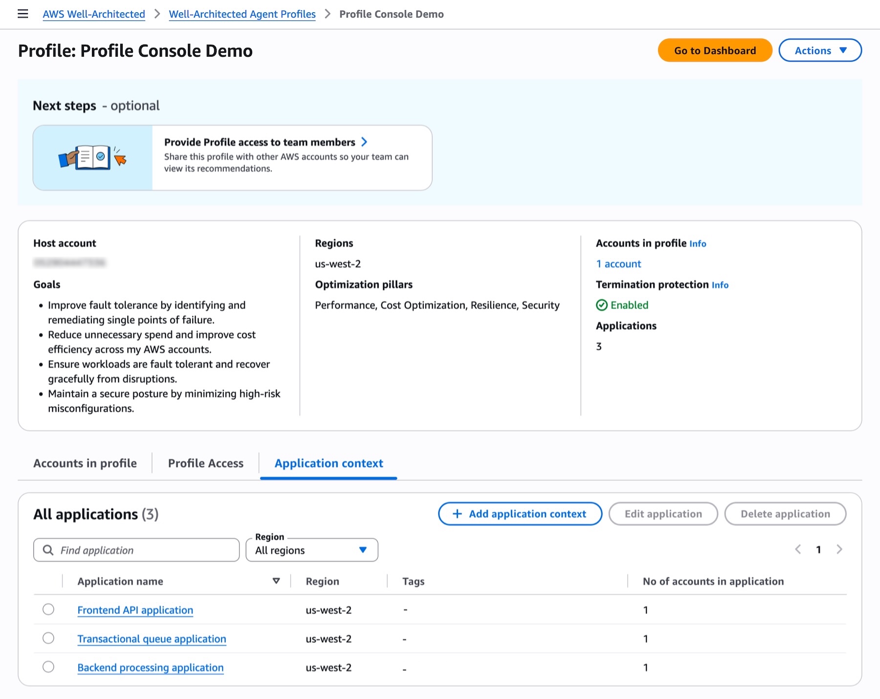
You can define your applications to add context which will enhance the relevancy and further contextualize recommendations. Choose Add application context in the dashboard, add your applications with AWS accounts, AWS Regions, AWS services, tags if you want to narrow the scope to specific resources, and the details of applications.
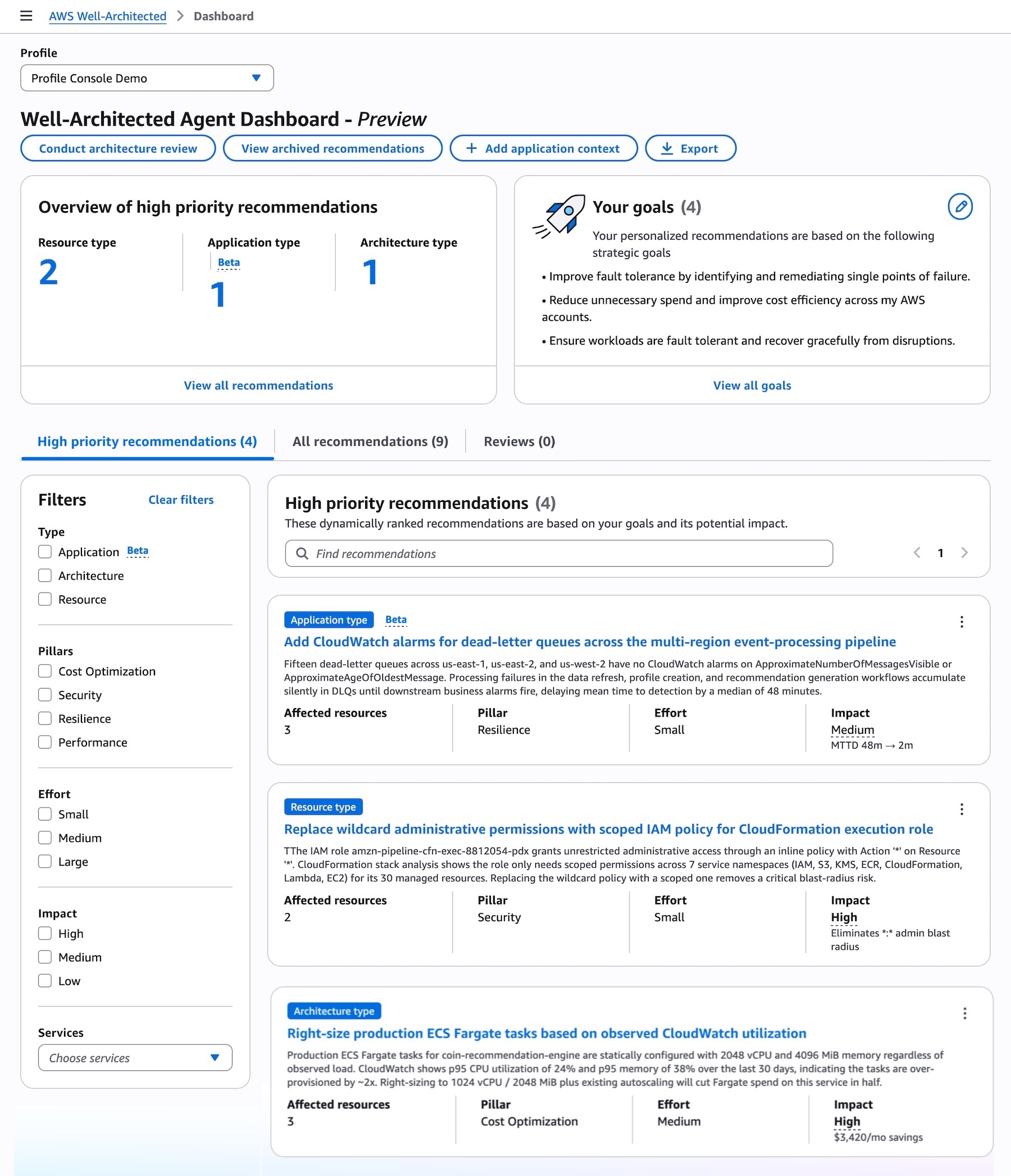
Review prioritized recommendations and start remediating

Now you can see generated prioritized recommendations generated by the agent across your resources and applications, selected pillars, ranked against your declared goals, with automation-ready remediation included.
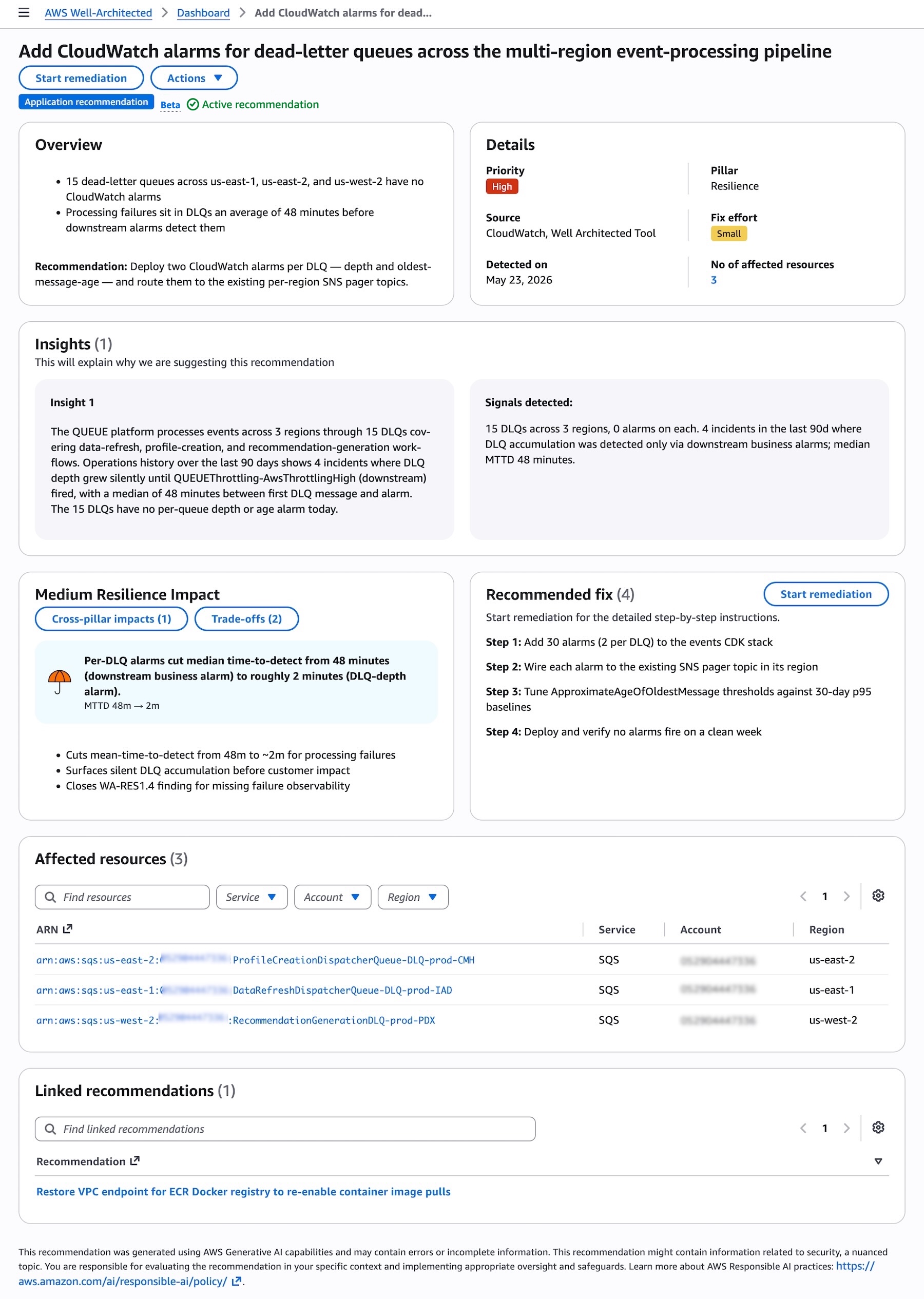
When you choose the specific recommendation, you can see the details, insights into why the agent are suggesting the recommendation, impacts and trade-off, and recommended fixes across affected AWS resources.
Choose Start remediation to address recommended fixes. You can choose the console, updated IaC template, CLI commands to remediate by the resolution type. It provides detailed step-by-step instructions and you can roll out this instruction and verify the result.
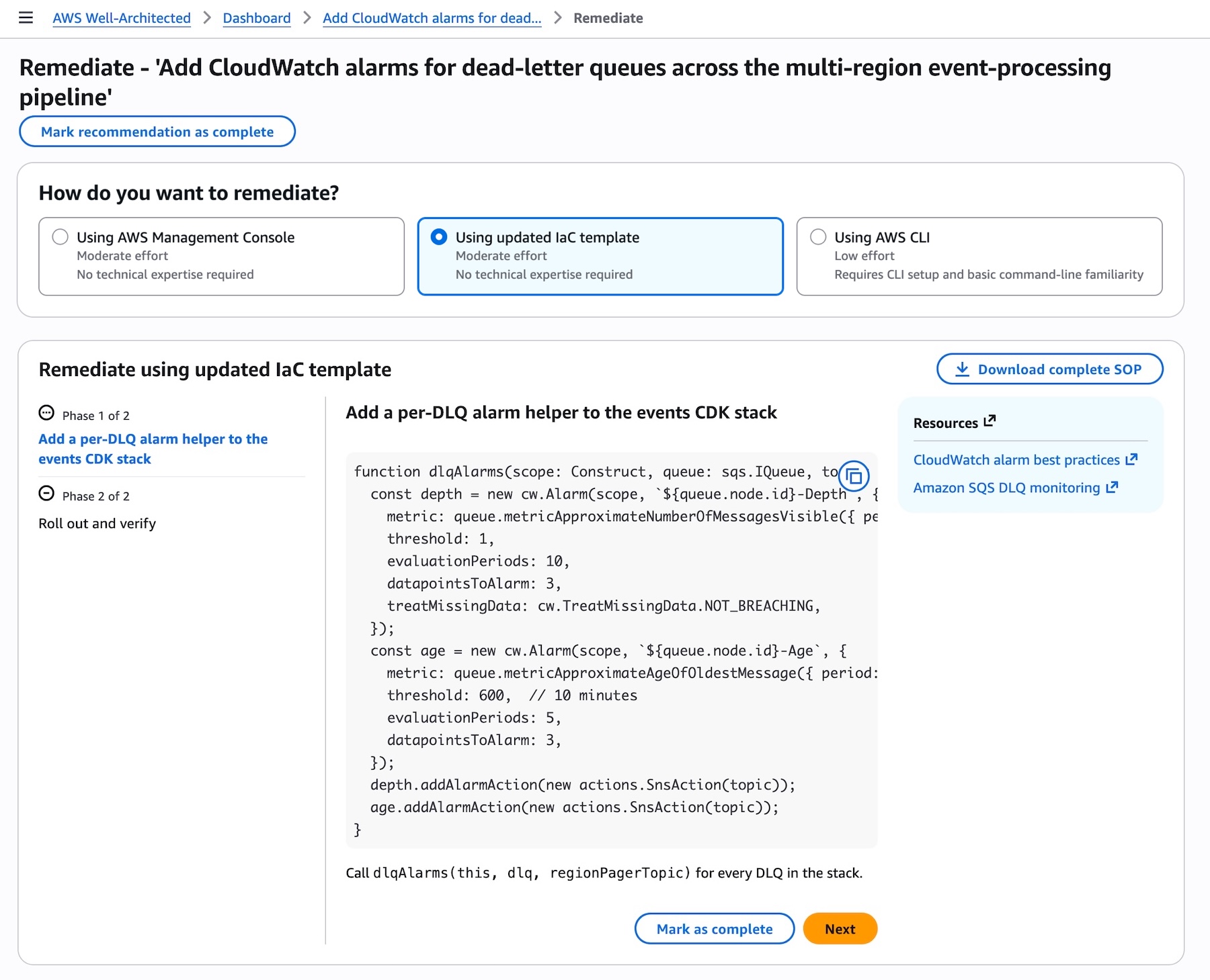
When you choose Using updated IaC template, the agent provides the code changes needed to update your existing IaC templates such as the CDK function shown above which you can copy directly into your codebase.

You can also configure API access to integrate recommendations directly into your existing development and operations workflows. To interact with the agent programmatically, including calling APIs and searching documentation, try the AWS MCP Server and plugins with your preferred AI coding tool. To learn more, visit the AWS Well-Architected Agent documentation.

Things to know

Here are some things that you should know about the Well-Architected Agent.

  • Automation: You can receive recommendations with the exact IaC code changes needed to remediate, with risks identified by pillar, catching issues before they reach production. Recommendations are delivered through the console and API so you can act without context-switching. Recommendations are also updated periodically, so new recommendations are available for your team to track regularly.
  • Evaluation: Generative AI capabilities produce this recommendation, which may contain errors or incomplete information. You are responsible for evaluating the recommendation in your specific context and implementing appropriate oversight and safeguards. Learn more about AWS Responsible AI practices.

You can still use existing AWS Well-Architected Tool to manually evaluate your cloud architecture with user-defined lenses that measure your workload using your own best practices.

Join the preview

Access to the AWS Well-Architected Agent and its recommendations is available in US East (N. Virginia), US East (Ohio), and US West (Oregon). You can onboard workloads from any AWS commercial Region. AWS Well-Architected Agent is delivered by AWS Support and available to AWS customers with an AWS Support plan.

Give it a try today in the AWS Well-Architected console and send feedback through your usual AWS Support contacts.

— Channy
Amazon S3 Tables now support all Apache Iceberg V3 data types

Post Syndicated from Daniel Abib original https://aws.amazon.com/blogs/aws/amazon-s3-tables-now-support-all-apache-iceberg-v3-data-types/

Amazon S3 Tables now support all data types in the Apache Iceberg V3 specification. You can create V3 tables or upgrade existing V2 tables to take advantage of V3 features like deletion vectors, row lineage, and new data types such as variant, nanosecond timestamps, unknown, geometry, and geography.

Apache Iceberg has become the open standard for managing large analytics datasets. It lets you manage petabyte-scale tables with features like schema evolution, hidden partitioning, and time travel queries, while keeping your data in open Parquet files in data lakes on object storage like Amazon S3. Amazon S3 Tables offer storage purpose-built to keep Iceberg tables performant and cost-effective as they grow, with fully managed features like automatic compaction, maintenance, replication, and Intelligent-Tiering.

Teams running analytics on Apache Iceberg V2 tables often hit the same limits as their data grows. A compliance request to delete 50,000 user records from a 2-billion-row table leaves behind positional delete files that slow queries until compaction runs. Semi-structured events land as JSON strings that every query has to parse. Geospatial coordinates and nanosecond-precision timestamps get encoded as strings or integers. Each workaround adds storage cost, query latency, and pipeline code. With V3, Iceberg solves these challenges by offering native support for semi-structured and geospatial data, faster row-level operations, and built-in row lineage for data governance.

Starting today, Amazon S3 Tables support all V3 data types, including variant, nanosecond timestamps, geometry, geography, and unknown, along with deletion vectors and row lineage. You can create new V3 tables or upgrade existing V2 tables in place, and S3 Tables continue to run compaction and maintenance for you.

Apache Iceberg V3

V3 is the latest version of the Iceberg specification. Among its many improvements, V3 introduces capabilities that address the most common pain points in V2. This includes:

Deletion vectors replace V2’s positional delete files with a compact binary format. That 50,000-row compliance delete now writes a single deletion vector file instead of thousands of small deletes, significantly reducing compaction time and delete file overhead.

Row lineage adds _row_id and _last_updated_sequence_number to each record automatically. Your downstream pipelines can query these fields to find changed rows without scanning the full table.

New data types let you store semi-structured, geospatial, and nanosecond-precision data natively instead of encoding it as strings or integers:

  • Nanosecond timestamp(tz) for nanosecond-precision timestamps
  • Geometry and geography for geospatial data
  • Unknown for columns with no known type

Variant data type stores semi-structured data in columnar format. During writes, the engine shreds variant data into hidden columns and collects statistics. At query time, those statistics enable file pruning that significantly reduces I/O compared to parsing JSON strings.

The following sections walk through how to use these V3 capabilities in practice, with examples that show how to create tables, work with the new data types, and manage data at scale.

Getting started

A retail analytics team tracks user behavior across web and mobile apps. Each event has a different structure: page views include URLs and duration, purchases include items and amounts, and searches include query terms and result counts. With V3’s variant type, you store all event shapes in one table without predefined schemas:

CREATE TABLE my_catalog.namespace.clickstream (
  event_id bigint,
  event_time timestamp,
  user_id string,
  payload variant
)
USING iceberg
TBLPROPERTIES ('format-version' = '3')

Insert events with different payload shapes without worrying about schema evolution:

INSERT INTO my_catalog.namespace.clickstream VALUES
  (1, current_timestamp(), 'user-42',
   PARSE_JSON('{"action": "purchase", "amount": 99.99, "items": ["laptop_stand"]}')),
  (2, current_timestamp(), 'user-17',
   PARSE_JSON('{"action": "page_view", "url": "/products/webcam", "duration_ms": 4200}'));

Now query the variant column directly, without PARSE_JSON at read time. With Amazon EMR Spark, use variant_get:

SELECT
  event_id,
  user_id,
  variant_get(payload, '$.action', 'string') AS action,
  variant_get(payload, '$.amount', 'double') AS amount
FROM my_catalog.namespace.clickstream
WHERE variant_get(payload, '$.action', 'string') = 'purchase'
  AND variant_get(payload, '$.amount', 'double') > 50.00

To enable deletion vectors for write operations, configure merge-on-read mode:

ALTER TABLE my_catalog.namespace.clickstream
SET TBLPROPERTIES (
  'write.delete.mode' = 'merge-on-read',
  'write.update.mode' = 'merge-on-read',
  'write.merge.mode' = 'merge-on-read'
)

Now when you run a compliance delete, V3 writes a small deletion vector instead of rewriting data files:

DELETE FROM my_catalog.namespace.clickstream
WHERE user_id = 'user-42'

S3 Tables compaction handles these deletion vector files automatically on the next maintenance cycle.

Upgrading from V2

AWS provides backwards compatibility for both versions to minimize disruption during migration to V3. Existing V2 readers continue to work on upgraded tables until you’re ready to fully adopt V3 features. For more details, see the S3 Tables Iceberg V3 documentation.

Upgrade an existing table atomically without rewriting data:

ALTER TABLE my_catalog.namespace.existing_table
SET TBLPROPERTIES ('format-version' = '3')

On the next compaction cycle, S3 Tables remove old V2 delete files. New modifications use deletion vectors automatically. Row lineage fields initialize on the first data modification after the upgrade.

This is a one-way operation. The Apache Iceberg specification does not support downgrading from V3 to V2. Verify that all engines accessing the table support V3 before upgrading.

Using row lineage for incremental pipelines

After your table has V3 data, use row lineage to build efficient incremental pipelines:

SELECT *, _row_id, _last_updated_sequence_number
FROM my_catalog.namespace.clickstream
WHERE _last_updated_sequence_number > 42

This returns only rows modified after sequence number 42. Your downstream jobs can checkpoint this value and process only new changes on each run, instead of scanning the full table.

Compatibility across AWS analytics services

AWS offers the broadest native Apache Iceberg support of any major cloud provider, with Iceberg-compatible services at every layer of the data stack: ingestion, storage, catalog, and analytics. You can store and automatically optimize V3 tables in Amazon S3 Tables, write data with Amazon EMR Spark, integrate and manage data with AWS Glue, and run analytics with Amazon Redshift. To learn more about AWS analytics support for V3, see the Apache Iceberg on AWS prescriptive guidance.

Both S3 Tables and AWS Glue Data Catalog support the Iceberg REST Catalog (IRC) API, enabling interoperability across engines regardless of the catalog endpoint.

Things to know

  • S3 Tables compaction fully supports V3 deletion vector files and preserves row lineage metadata.
  • The new V3 data types (variant, nanosecond timestamps, geometry, geography, and unknown) require an engine built on Apache Spark 4.0 or later, such as AWS Glue 6.0 or later, or Amazon EMR release 8.1 or later.
  • You can create V3 tables from the Amazon S3 console, AWS CLI, or any engine that supports the Iceberg REST Catalog API.
  • The new V3 data types are supported only for tables that use the Parquet file format (not ORC or Avro).
  • Columns of type variant, geometry, geography, or nanosecond timestamp can’t be included in a table’s sort order for compaction. Tables containing these columns still compact under the sort and Z-order strategies when the sort order uses columns of other types.

Now available

Amazon S3 Tables support for all Apache Iceberg V3 data types is now available in all AWS Regions where S3 Tables are supported. Apache Iceberg V3 support is available at no additional charge; standard S3 Tables pricing applies.

To get started, visit the Amazon S3 Tables documentation or create a table bucket from the Amazon S3 console. If you want to call APIs, search documentation, find regional availability, and check troubleshooting about this feature, try using the AWS MCP Server and plugins with your preferred AI tool. Send feedback to AWS re:Post or through your usual AWS Support contacts.

– Daniel Abib

Amazon S3 Vectors now supports metadata pre-filtering for higher recall on filtered searches

Post Syndicated from Daniel Abib original https://aws.amazon.com/blogs/aws/amazon-s3-vectors-now-supports-metadata-pre-filtering-for-higher-recall-on-filtered-searches/

Today, we’re announcing metadata pre-filtering for Amazon S3 Vectors, which delivers higher recall on filtered queries by evaluating your metadata filter before the similarity search. You can filter on attributes such as tenant, category, status, or time, and pre-filtering adds prefix matching with $startsWith for paths, URLs, and hierarchical keys. Each vector carries up to 2 KB of filterable metadata, and a single query supports up to 100 filter constraints. There is no additional cost, no re-ingestion, and no change to your queries.

Most applications never search a whole index. They search the part of it that belongs to a particular user, account, or category, and they express that scope as a metadata filter. Semantic search, retrieval-augmented generation (RAG), and agentic applications all need the same thing from a filtered query: a similarity search that covers the vectors matching the filter, and returns the closest of them. With pre-filtering, a filtered query returns more of the relevant matches your index contains, giving you higher recall on filtered searches.

Common use cases

Pre-filtering applies wherever results have to be both relevant and correctly scoped:

  • Legal and professional services: A law firm or e-discovery platform searches documents scoped to a single client, and with $startsWith narrows further by matter number, folder path, or document ID prefix. A single client is a small share of a firm-wide archive, and filters this narrow are where pre-filtering improves recall most.
  • Financial services: An investment research platform searches analyst notes, filings, and call transcripts scoped by issuer, document type, and publication date.
  • Media and entertainment: A streaming service filters by content rating and regional licensing before the semantic search, finding similar titles restricted to G and PG content licensed in one territory.
  • Agentic applications: An agent working within a user’s session filters on fields such as owner, document set, and timestamp so its searches cover the material relevant to the task at hand. Higher recall means more of that material reaches the agent, which improves task reliability

How pre-filtering works

Each vector in an S3 Vectors index can carry application-defined metadata, and a query can filter on those fields.

Every vector index has an index mode. On an index whose index mode is ENHANCED, S3 Vectors resolves your filter first, then searches only the vectors that match. On an index whose index mode is CLASSIC, S3 Vectors performs the vector search and filter evaluation in tandem, validating each candidate vector against your filter as it searches. Existing indexes use CLASSIC until you update them.

Consider a support knowledge base of 8 million tickets, where an agent searches one customer’s history for a recurring error. If that customer accounts for 400 of those tickets, resolving customer_id first means the similarity search runs across all 400 of them, so the agent sees that customer’s prior occurrences. Before the index was updated, the same query drew its candidates from the full 8 million, and the result set contained fewer of that customer’s matching tickets.

On highly selective filters, pre-filtering returns up to 5x more of the matching vectors than the same query returned before on CLASSIC indexes.

Getting started

Before you start, make sure your IAM policy grants permissions for the new actions.

You can get started in three steps. The walkthrough below builds a small product-catalog index and runs a selective filter against it, the same pattern you would use for a multi-tenant RAG store or a document search scoped to one client.

First, create a vector index:

aws s3vectors create-index \
  --index-name product-catalog \
  --vector-bucket-name my-vector-bucket \
  --dimension 1536 \
  --distance-metric cosine

The dimension must match the output size of your embedding model, and distance-metric should match how that model was trained (cosine is common for text embeddings). Second, write vectors with the PutVectors API, attaching up to 2 KB of filterable metadata to each vector:

aws s3vectors put-vectors \
  --index-name product-catalog \
  --vector-bucket-name my-vector-bucket \
  --vectors '[{
    "key": "doc-001",
    "data": {"float32": [0.1, 0.2, 0.3, ...]},
    "metadata": {
      "tenant_id": "t-10428",
      "category": "legal",
      "created_date": "2026-03-15",
      "active": true
    }
  }]'

Each vector carries the attributes your application filters on. In this example, tenant_id scopes results to a single customer, category narrows by document type, created_date records when the document was created, and active is a boolean flag. By default every metadata field is filterable, so you can query on any of them without declaring a schema up front.

Third, run a filtered similarity query with the QueryVectors API. The filter uses a compact JSON syntax where a bare key-value pair is an equality match, and operators such as $and, $or, and $gt combine or refine conditions. Pass --return-metadata so the query returns each vector’s metadata:

aws s3vectors query-vectors \
  --index-name product-catalog \
  --vector-bucket-name my-vector-bucket \
  --query-vector '{"float32": [0.1, 0.2, 0.3, ...]}' \
  --top-k 50 \
  --return-metadata \
  --filter '{"$and": [
    {"tenant_id": "t-10428"},
    {"category": "legal"},
    {"active": true}
  ]}'

The expected result is a single vector, doc-001, the only one matching all three filter conditions (tenant_id, category, and active):

{
  "vectors": [
    {
      "distance": 0.9717477560043335,
      "key": "doc-001",
      "metadata": {
        "tenant_id": "t-10428",
        "category": "legal",
        "created_date": "2026-03-15",
        "active": true
      }
    }
  ],
  "distanceMetric": "cosine"
}

S3 Vectors first narrows the search space to vectors matching all three filter conditions, then returns the 50 most similar vectors from that subset. Because the filter is applied before the search, those results are drawn from across all the vectors that match it.

Prefix matching with $startsWith

Pre-filtering adds a prefix match operator for filtering on paths, URLs, and hierarchical keys. A document store that encodes case and folder structure into a document ID can scope a search to a subtree in one condition:

--filter '{"$startsWith": {"document_id": "matter-4417/exhibits/"}}'

$startsWith joins the existing operators: equality, numeric range, set membership, existence checks, and boolean logic with $and and $or.

Turning on pre-filtering for existing indexes

Call UpdateIndexMode on an existing index to turn on pre-filtering:

aws s3vectors update-index-mode \
  --vector-bucket-name my-vector-bucket \
  --index-name product-catalog \
  --index-mode ENHANCED

Pre-filtering takes effect in place. Your existing vectors are not re-ingested, your queries do not change, and the new filter operators are available immediately.

Here is the difference on the same index and the same query. Before the update, a query scoped to one tenant returns two of the ten results requested:

aws s3vectors query-vectors \
  --vector-bucket-name my-vector-bucket \
  --index-name product-catalog \
  --query-vector '{"float32": [0.1, 0.2, 0.3, ...]}' \
  --top-k 10 \
  --return-metadata \
  --filter '{"tenant_id": "t-10428"}'
{
  "vectors": [
    { "key": "doc-114", "distance": 0.41 },
    { "key": "doc-322", "distance": 0.55 }
  ],
  "distanceMetric": "cosine"
}

After the update, the same query returns a full result set drawn from across that tenant’s documents:

{
  "vectors": [
    { "key": "doc-018", "distance": 0.09 },
    { "key": "doc-207", "distance": 0.13 },
    { "key": "doc-114", "distance": 0.41 },
    ... 7 more
  ],
  "distanceMetric": "cosine"
}

Rolling out across your indexes

Once you have validated pre-filtering on an index, set the default index mode on the vector bucket so that new indexes use ENHANCED without a follow-up call:

aws s3vectors put-vector-bucket-default-index-mode \
  --vector-bucket-name my-vector-bucket \
  --default-index-mode ENHANCED

To bring the rest of your existing indexes across, list them and check the index mode on each one, then call UpdateIndexMode on the ones still using CLASSIC:

aws s3vectors list-indexes \
  --vector-bucket-name my-vector-bucket

aws s3vectors get-index \
  --vector-bucket-name my-vector-bucket \
  --index-name product-catalog

Things to know 

  • Indexes created in vector buckets created on or after September 30, 2026 use index mode ENHANCED. Indexes in buckets that existed before that date use CLASSIC until you set the bucket default, including indexes created in those buckets afterward.
  • A single query supports up to 100 filter constraints, counted per value the filter evaluates. If a query exceeds that, you can usually consolidate the filter, replacing a 300-value $in over legal cases with a single caseId field, for example, or split it into smaller queries, run them in parallel, and merge the results by distance.

Get started today

Metadata pre-filtering is available at no additional cost in all commercial AWS Regions where Amazon S3 Vectors is available, and in the AWS China Regions. You pay standard S3 Vectors pricing for storage, PUT requests, and queries. For full pricing details, visit the Amazon S3 pricing page. For regional availability, visit Amazon S3 Vectors Regions and quotas.

Whether you’re scoping a RAG application to one tenant, scoping an agent’s searches to one user’s documents, or narrowing a catalog search to a licensing window, pre-filtering lets you apply those filters without trading away recall. To learn more and get started, visit the Amazon S3 Vectors documentation. Send feedback to AWS re:Post for S3 or through your usual AWS Support contacts.

— Daniel Abib

Amazon Aurora PostgreSQL now supports direct querying of Apache Iceberg and Parquet data in your data lake

Post Syndicated from Esra Kayabali original https://aws.amazon.com/blogs/aws/amazon-aurora-postgresql-now-supports-direct-querying-of-apache-iceberg-and-parquet-data-in-your-data-lake/

Today, we’re announcing a new capability for Amazon Aurora PostgreSQL that you can use to directly query operational data together with data stored in your data lake in Apache Iceberg and Apache Parquet formats, using your existing PostgreSQL applications and tools. By eliminating the need to extract, transform, and load (ETL) structured data from data lakes into your operational database, you can reduce operational complexity and simplify application development. You can also use Aurora PostgreSQL to query data from data lakes managed in Iceberg REST Catalog (IRC)-compatible catalogs, giving you access to data across a breadth of analytics systems without moving or duplicating it. Whether you’re powering real-time dashboards, enriching transactions with historical context, or building AI agents that reason over both live and archived data, you can now do it all through a single, familiar interface.

Previously, if your application needed to combine recent transactional data in Aurora with historical records stored in Amazon S3, a common approach was to build reverse ETL pipelines that duplicated data, increased infrastructure costs, and required ongoing engineering effort to keep everything synchronized. This challenge only grows as you increasingly embed AI agents into your applications, where it is impractical to predict and pre-replicate every dataset an agent might need.

DuckLabs, the team that maintains the DuckDB project, recently joined Amazon, and this capability is an example of how the efficiency of DuckDB is being integrated into our services. DuckDB is now embedded directly within Aurora PostgreSQL, so you can query live operational data (including uncommitted writes) alongside your data lake in a single query. Query processing stays within Aurora, with no additional network hops and no ETL pipelines that duplicate data. You can query Apache Iceberg tables managed through the AWS Glue Data Catalog, as well as Parquet and Iceberg data stored in Amazon S3 and S3 Tables. You do all of this using familiar PostgreSQL syntax and your existing applications and tools.

We’re excited to bring the speed and simplicity of DuckDB directly into Aurora PostgreSQL, so you and your agents can query and combine operational and Iceberg data using the familiar PostgreSQL applications, tools, and endpoints already in use. By building this capability around DuckDB, future improvements to the open source engine can continue to bring performance and functionality gains to Aurora and other AWS services.

What is new

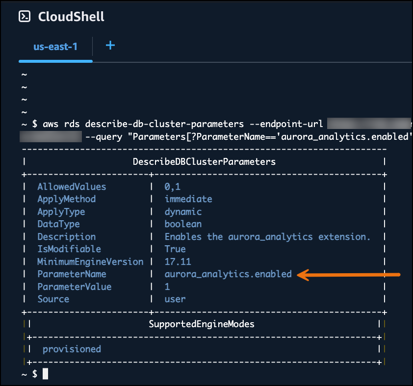
This capability is supported on two Aurora PostgreSQL major versions: 17 (starting with 17.11) and 18 (starting with 18.6). To use it, you create an Aurora PostgreSQL cluster, attach an IAM role with the AuroraAnalytics feature, and enable the aurora_analytics extension. The IAM role is what gives Aurora access to your data in Amazon S3 and the AWS Glue Data Catalog. You then create foreign tables that point to your Iceberg or Parquet data in the data lake, and query them using familiar PostgreSQL syntax. You can complete this setup through the Amazon RDS console, or with any PostgreSQL client such as psql. The process is well documented in the Aurora PostgreSQL documentation.

You can query data across external IRC-compatible catalogs through AWS Glue Data Catalog federation. You register the external catalog once with Glue, and then create foreign tables for the tables you want to query, the same way you would for any Glue-native table. A single query can then join data stored in Aurora with Iceberg tables registered across multiple catalogs, so applications get a unified view without moving data or replacing your existing catalog investments.

Aurora also applies optimizations such as predicate pushdown and column pruning so that only the relevant data is read. This keeps queries efficient even as the underlying data grows. Frequently accessed data is also cached in your Aurora instance, so subsequent queries against the same data return faster. You can inspect this behavior per query using aurora_analytics_stat_statements(), which reports metrics such as rows scanned, bytes read from Amazon S3, and cache hits.

To see how direct querying works, I connected to my Aurora PostgreSQL database using psql and created the extension:

CREATE EXTENSION aurora_analytics;

For my walkthrough, I set up a simple financial scenario. I have a recent_transactions table in Aurora with the last 7 days of customer transactions, and a Parquet file in Amazon S3 containing 5 years of historical transaction data. To make Aurora aware of the historical data, I created a foreign table pointing at the Parquet file in S3:

CREATE FOREIGN TABLE transaction_history ()
SERVER aurora_analytics_server
OPTIONS (
    location 's3://<my-bucket>/finance/transaction_history.parquet',
    format 'parquet'
);

Notice the empty parentheses in the CREATE FOREIGN TABLE statement. Aurora automatically reads the schema from the Parquet file metadata, so you do not need to define columns manually. For workloads with many tables, you can skip creating them one at a time: a single IMPORT FOREIGN SCHEMA statement bulk-creates foreign tables for every Iceberg or Parquet table in an AWS Glue Data Catalog database, inferring schemas automatically.

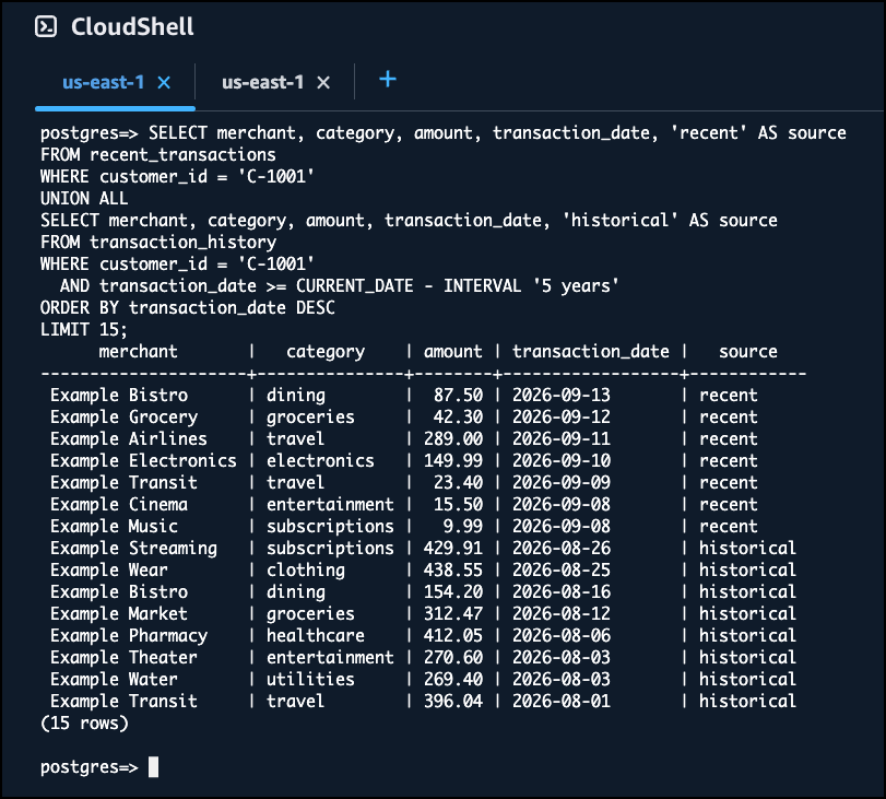
With both tables in place, I ran a single query that combines the recent operational data in Aurora with the historical data in S3:

SELECT merchant, category, amount, transaction_date, 'recent' AS source
FROM recent_transactions
WHERE customer_id = 'C-1001'
UNION ALL
SELECT merchant, category, amount, transaction_date, 'historical' AS source
FROM transaction_history
WHERE customer_id = 'C-1001'
  AND transaction_date >= CURRENT_DATE - INTERVAL '5 years'
ORDER BY transaction_date DESC
LIMIT 15;

The result shows both recent and historical transactions in a single result set. The 7 most recent rows come from Aurora, and the rest come directly from the Parquet file in S3. DuckDB handles the analytical scan of the Parquet data under the hood, while Aurora handles the operational data. That single query would have previously required a pipeline to move the historical data into the database first.

If a query pattern needs single-digit-millisecond latency, you can materialize data from the data lake into a native Aurora PostgreSQL table using familiar commands such as CREATE TABLE AS SELECT, INSERT INTO ... SELECT, or MERGE INTO. The materialized table lives in Aurora and is queried like any other PostgreSQL table, giving you a low-latency path for hot data without operating a separate ingestion pipeline. The read queries can run on any Aurora PostgreSQL instance in your cluster, whether the writer or a read replica, so you can offload analytical scans from your operational workload. The materialization commands write data into Aurora, so they run on the writer instance.

Get started today

Direct querying of Apache Iceberg and Parquet data from Amazon Aurora PostgreSQL is available today in all commercial AWS Regions and AWS GovCloud (US) Regions, at no additional charge. You pay only for the incremental Aurora compute the queries consume and Amazon S3 request costs for reading data lake files.

To learn more, visit the Amazon Aurora features page, read the Aurora PostgreSQL documentation, or try it in the Amazon RDS console. We welcome your feedback through AWS re:Post or through your usual AWS Support contacts.

— Esra

Celebrating Our Newest AWS Heroes – September 2026

Post Syndicated from Taylor Jacobsen original https://aws.amazon.com/blogs/aws/celebrating-our-newest-aws-heroes-september-2026/

Today, we’re excited to introduce the newest members of the AWS Heroes program. AWS Heroes are a vibrant, worldwide group of AWS experts who go above and beyond to share knowledge, mentor others, and build thriving communities. These individuals make a real difference in helping developers and organizations succeed with AWS.

This month, we welcome three exceptional community leaders from across the globe, each bringing unique expertise and a deep commitment to empowering builders everywhere.

Avinash Shashikant Dalvi – Bengaluru, India

Serverless Hero Avinash Shashikant Dalvi is a tech architect and co-organizer of AWS User Group Bengaluru who is focused on serverless, containers, and production-ready applications on AWS. He has delivered over 40 community talks, publishes the AWS for Product Builders newsletter, and creates technical content covering Amazon ECS, AWS Fargate, AWS Lambda, and AWS Amplify.

Joanne Skiles – Orlando, USA

Serverless Hero Joanne Skiles is an engineering leader and educator with over 16 years of experience building full-stack systems, including serverless architecture and AI systems on AWS. She organizes the Orlando AWS User Group and teaches cloud and AI concepts through her YouTube channel, conference talks, and her podcasts Chaotic Commits and Her Career Unplugged. Joanne is also a professor in the Computer Science department at Rollins College, where she runs the Transparent Systems lab.

Xiaofei Li – Shanghai, China

Community Hero Xiaofei Li is an AWS Golden Jacket holder and is an active community leader in the Greater China Region, leading the Kiro, Amazon Quick, and Tokyo Chinese AWS communities. He founded the Kiro Chinese User Community (5,000+ members) and initiated the Chinese localization of AWS Builder Cards across 15 cities and 3,000+ participants. Xiaofei also mentors underserved students and supports Women in Tech initiatives.

Learn More

Visit the AWS Heroes webpage if you’d like to learn more about the AWS Heroes program, or to connect with a Hero near you. To learn more about how to get involved with the AWS community, visit our AWS Builder Center.

— Taylor

Introducing enhanced custom event buses in Amazon EventBridge for enterprise-scale event-driven applications

Post Syndicated from Micah Walter original https://aws.amazon.com/blogs/aws/introducing-enhanced-custom-event-buses-in-amazon-eventbridge-for-enterprise-scale-event-driven-applications/

Organizations building event-driven applications on Amazon EventBridge typically start with a single custom event bus in one account. This works well when a single team owns the architecture. As adoption grows across the organization, though, things get complicated. AWS best practices recommend a multi-account structure, which means each team runs in its own account. To route events between them, teams create multiple event buses connected through cross-account rules or bus-to-bus configurations. This workaround reintroduces the operational complexity that serverless architectures are meant to eliminate. Platform teams lose visibility into who is subscribing to which events, cross-account and bus-to-bus routing charges compound quickly, and teams that need capabilities like event ordering are forced to build complex workarounds or adopt entirely different technologies.

Today, we are announcing an enhanced custom event bus in Amazon EventBridge, purpose-built for organizations scaling event-driven applications across teams and accounts. With the new enhanced custom event bus, you can deploy a single, centralized event bus shared across all AWS accounts in your organization, with ordering guarantees, a simplified Subscriber resource, and a new pricing model that delivers improved economics at scale and cost allocation for publishers and subscribers.

Let’s try it out

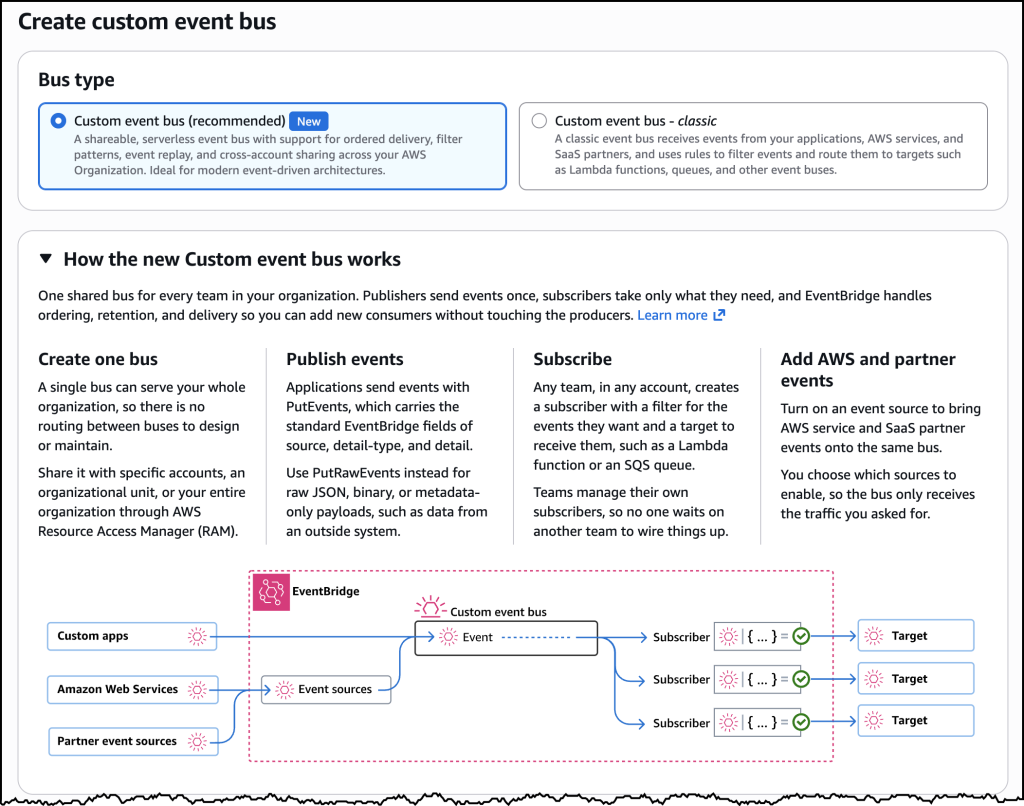
To get started with an enhanced custom event bus, I navigated to the EventBridge console in the AWS Management Console and opened the Create custom event bus page. I selected Custom event bus, the recommended option labeled New. The page also offered Custom event bus – classic, which continues to receive events and route them with rules and targets. Below the selection, EventBridge showed how the new bus works. One shared bus serves every team in the organization. Publishers send events, subscribers consume only what they need, and EventBridge handles ordering, retention, routing, and delivery.

The Create custom event bus page. Custom event bus is the recommended new option, with ordered delivery, filter patterns, event replay, and sharing across your AWS organization. Custom event bus – classic remains available for existing workloads.

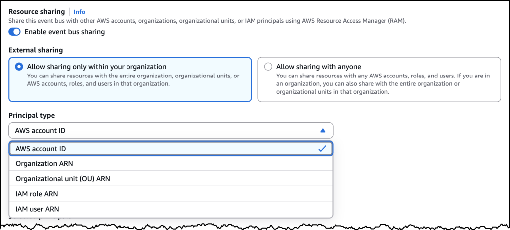
Next, I configured resource sharing. I turned on Enable event bus sharing and selected Allow sharing only within your organization. I chose AWS account ID as the principal type. I could also share with an organization, an organizational unit, or an AWS Identity and Access Management (IAM) role or user. Sharing uses AWS Resource Access Manager (AWS RAM), so I did not have to set up cross-account permissions or bus-to-bus routing myself.

Resource sharing on the new custom event bus. I enabled sharing within my organization through AWS RAM and selected an AWS account as the principal, which is how teams publish and subscribe on the same bus without extra routing.

Organization-wide sharing

With the new enhanced custom event bus, you can create a single event bus and share it across all AWS accounts in your organization. Platform teams deploy one bus and establish it as the central event backbone, eliminating the need to configure cross-account permissions or bus-to-bus routing. Application teams across your organization can publish and subscribe to events on the same bus without waiting for infrastructure provisioning.

Publishers send events without needing to know which teams consume them, and subscribers create their own Subscriptions independently. Platform teams maintain visibility into all event flows and fine-grained control over who can publish and consume events. The new enhanced custom event bus has a default quota of 10,000 Subscribers per bus, and you can request a higher quota. That reduces the fragmentation that occurs when subscriber limits force you to split across multiple buses.

Event ordering

Event-driven architectures work best when consumers are designed around asynchronous patterns, where the order of events does not matter. There are a few cases where order does matter. In a logistics application, driver location updates must arrive in sequence. Out-of-sequence events cause routing algorithms to make decisions based on stale data.

The enhanced custom event bus supports both patterns on the same bus. Publishers can include an EventGroupId when sending events. EventBridge delivers events that share the same EventGroupId in sequence to Subscribers that chose ordered delivery. Other subscribers on that bus can receive the same events without ordering. You can keep events for each driver in the correct order without building complex workarounds, while the rest of your consumers stay fully asynchronous.

To support ordered processing, the enhanced custom event bus includes synchronous invocation for targets like AWS Lambda. Synchronous mode confirms successful processing before acknowledging the event, eliminating the common pattern of placing Amazon Simple Queue Service (Amazon SQS) between an event bus and Lambda to ensure reliability.

Subscriptions

The enhanced custom event bus introduces the Subscriber resource, which combines event filtering, target configuration, retry policies, and dead-letter destinations into a single, manageable unit. Today, achieving the same outcome with EventBridge requires configuring separate rules, targets, and retry settings across multiple resources. Subscribers simplify this by giving each consumer one resource that defines what events they want, where to deliver them, and how to handle failures.

Subscribers also include variable start time options, making it easier for teams to onboard new consumers or replay events to recover from application errors or hydrate new applications.

Event evaluation

Publishers can turn on content-based deduplication so EventBridge detects and drops retries of the same event from the payload itself. You do not have to generate and track a deduplication ID when a timeout or a partial failure sends the same event twice. EventBridge hashes the meaningful parts of the event and collapses matches that arrive within five minutes, which gives those retries exactly-once delivery semantics instead of EventBridge’s usual at-least-once model. If you already stamp your own idempotency token, keep using it. Content-based deduplication is for sources that cannot reliably identify the same event on a retry.

Subscribers can use JSONata expressions to reshape an event before it reaches a target, extracting fields, renaming them, or computing new values when a downstream API expects a different shape. If you already produce Apache Avro or Protocol Buffers events, EventBridge can deserialize those payloads to JSON, allowing subscribers fine grained filtering and routing on the full event payload without having to consume, deserialize, and match or discard on their own.

New pricing model

The enhanced custom event bus uses a new ingress and egress throughput pricing model. Publishers pay for events ingested, and subscribers pay for events delivered. This replaces the per-event model where cross-account and bus-to-bus routing charges compound in multi-bus architectures. For pricing details, visit the EventBridge pricing page.

Existing EventBridge custom event buses continue to work as they do today with no changes required. They now appear as Custom event bus – classic. The enhanced custom event bus is a new resource that you adopt at your own pace. In the console, it appears as Custom event bus.

Now available

The enhanced custom event bus is available today in the US East (N. Virginia, Ohio), US West (Oregon), Europe (Ireland, Frankfurt, Stockholm, Spain), and Asia Pacific (Hong Kong, Malaysia, Mumbai, Singapore, Sydney, Thailand, Tokyo) Regions. You can create your first enhanced custom event bus through the AWS Management Console, AWS Command Line Interface (AWS CLI), or EventBridge APIs. To get started, visit the EventBridge documentation or try it out directly in the EventBridge console.

Introducing Amazon CloudWatch Omni: collaborative AI-powered observability for your applications

Post Syndicated from Daniel Abib original https://aws.amazon.com/blogs/aws/introducing-amazon-cloudwatch-omni-collaborative-ai-powered-observability-for-your-applications/

Amazon CloudWatch now offers CloudWatch Omni, an AI-powered observability experience for the applications and AI agents you run together. You reach Omni through a dedicated URL for your organization and sign in with the identities you already manage, so working in Omni does not require access to the AWS Management Console. Omni is built on OpenTelemetry: the telemetry you already send to CloudWatch appears in Omni with nothing to reconfigure, and any other workload you instrument with OpenTelemetry sends its telemetry to an OpenTelemetry Protocol (OTLP) endpoint.

CloudWatch Omni offers both agent observability and application observability in a single experience. In our companion post, we introduced the agent observability capabilities of Omni for generative AI and agentic workloads. In this post, we present the application observability experience.

Engineering teams spend a significant portion of their observability time maintaining dashboards, tuning thresholds, and switching between tools to piece together what happened during an incident. When an issue crosses team boundaries, context gets lost in Slack threads and screenshots rather than flowing naturally to the next engineer. CloudWatch Omni changes this by organizing observability around your applications rather than individual signals, and bringing your whole team into the same workspace.

What CloudWatch Omni brings

CloudWatch Omni addresses three problems that engineering teams told us they face today.

One collaborative experience for your whole team. Every engineer accesses CloudWatch Omni through a single URL with enterprise SSO (via IAM Identity Center, supporting Okta, Azure AD, and other providers). No AWS Console access is required. SREs, developers, database engineers, and managers share the same data and investigation context. When an investigation escalates, the next person joins the same session with full context already in front of them.

The system adapts as your applications evolve. CloudWatch Omni discovers your services, maps dependencies, and adjusts alarms automatically. Instead of manually curating dashboards and tuning thresholds, you declare what matters (availability targets, latency budgets, error rate thresholds) and Omni adapts as your system changes. When you deploy new services, Omni updates the application topology automatically.

AI-powered investigation with Amazon DevOps Agent. Amazon DevOps Agent participates alongside your team in investigation sessions, correlating signals and suggesting next steps. The agent works from the same telemetry your engineers see, so its suggestions are grounded in the actual state of your application. It identifies correlated events across services, traces root cause paths through your dependency graph, and maintains investigation history for post-incident review.

How an investigation works

When something breaks, CloudWatch Omni opens an investigation session pre-loaded with context. Here is a typical incident workflow:

An alarm fires on elevated error rates in your checkout service. Omni opens a session showing the service topology, correlated signals (a deployment 10 minutes earlier, increased latency from a downstream payment API), and DevOps Agent’s initial analysis.

Your on-call SRE confirms the deployment correlation, pulls in the trace view to identify failing endpoints, and checks if the payment API latency correlates with a capacity limit.

The SRE escalates to the payments team. The payments engineer joins the same session and sees everything found so far, plus DevOps Agent’s correlation with a configuration change in the payment provider’s API gateway. They identify the root cause and roll back.

The entire investigation history is captured automatically. No separate incident report needed.

Walkthrough: setting up your first Space

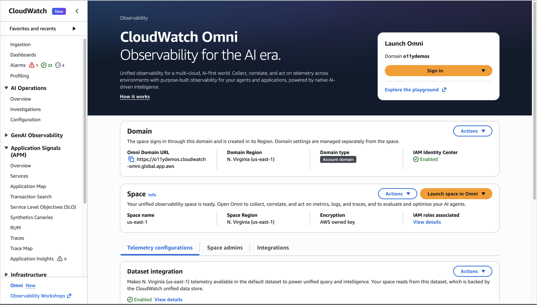
To set up CloudWatch Omni for your team, open the CloudWatch console and click “Try CloudWatch Omni.”


Figure 1. CloudWatch console — Omni setup page

Next, connect your identity provider through IAM Identity Center (supporting Okta, Azure AD, and other SAML 2.0 providers). Once connected, your team members access Omni directly at your dedicated URL without needing AWS Console credentials.

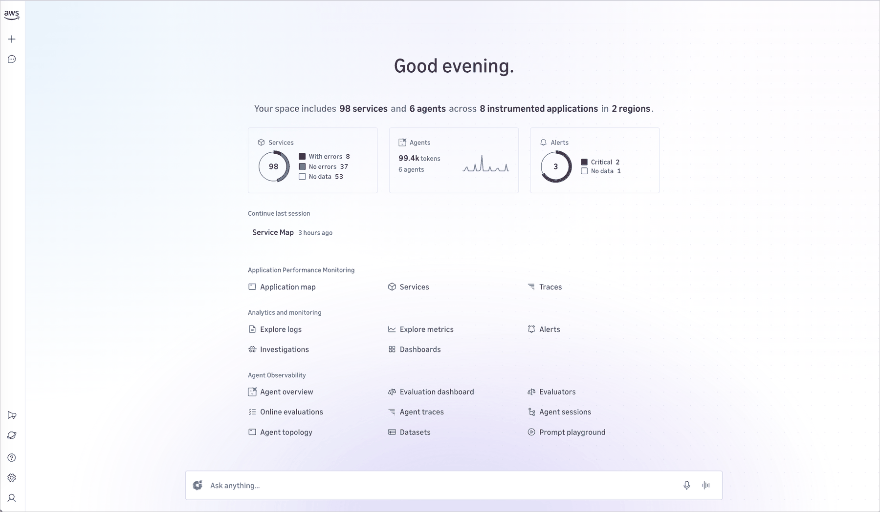
Create a Space for your team. A Space groups the applications your team owns and the telemetry associated with them.


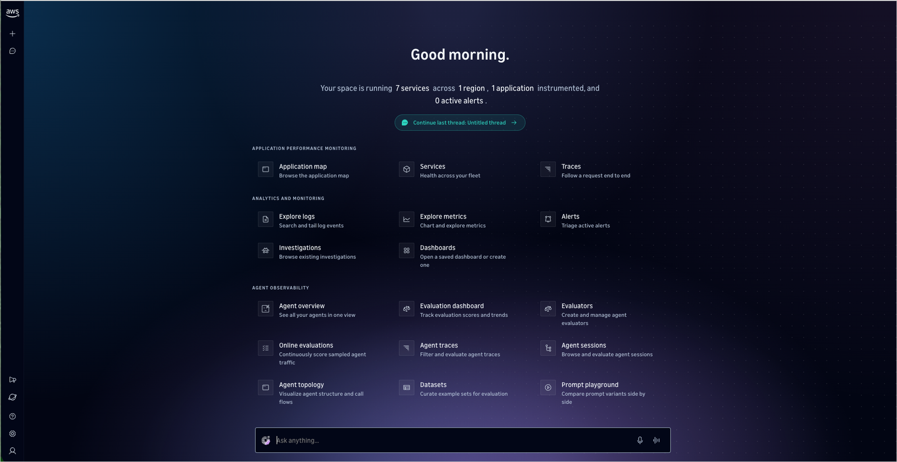
Figure 2. CloudWatch Omni Home — your team’s workspace with application monitoring, analytics, and agent observability

Once created, Omni discovers your services automatically and maps the dependencies between them. You see your application topology immediately.


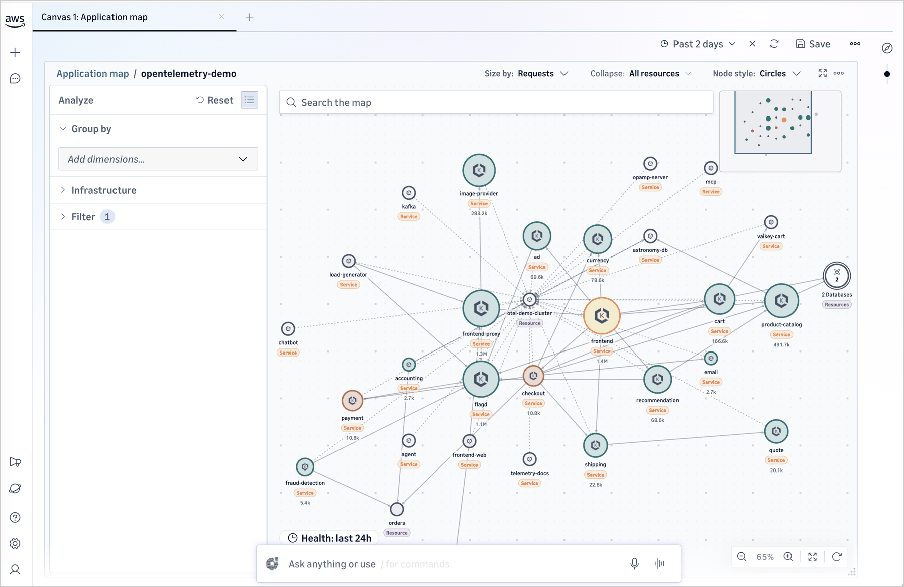
Figure 3. Application topology — services and dependencies mapped automatically

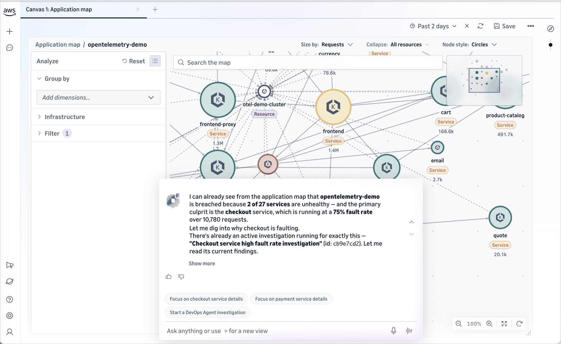
You can ask CloudWatch Omni any question about your applications in plain English, and Omni will analyze your telemetry data and surface insights.

Figure 4. Interact with your telemetry in natural language

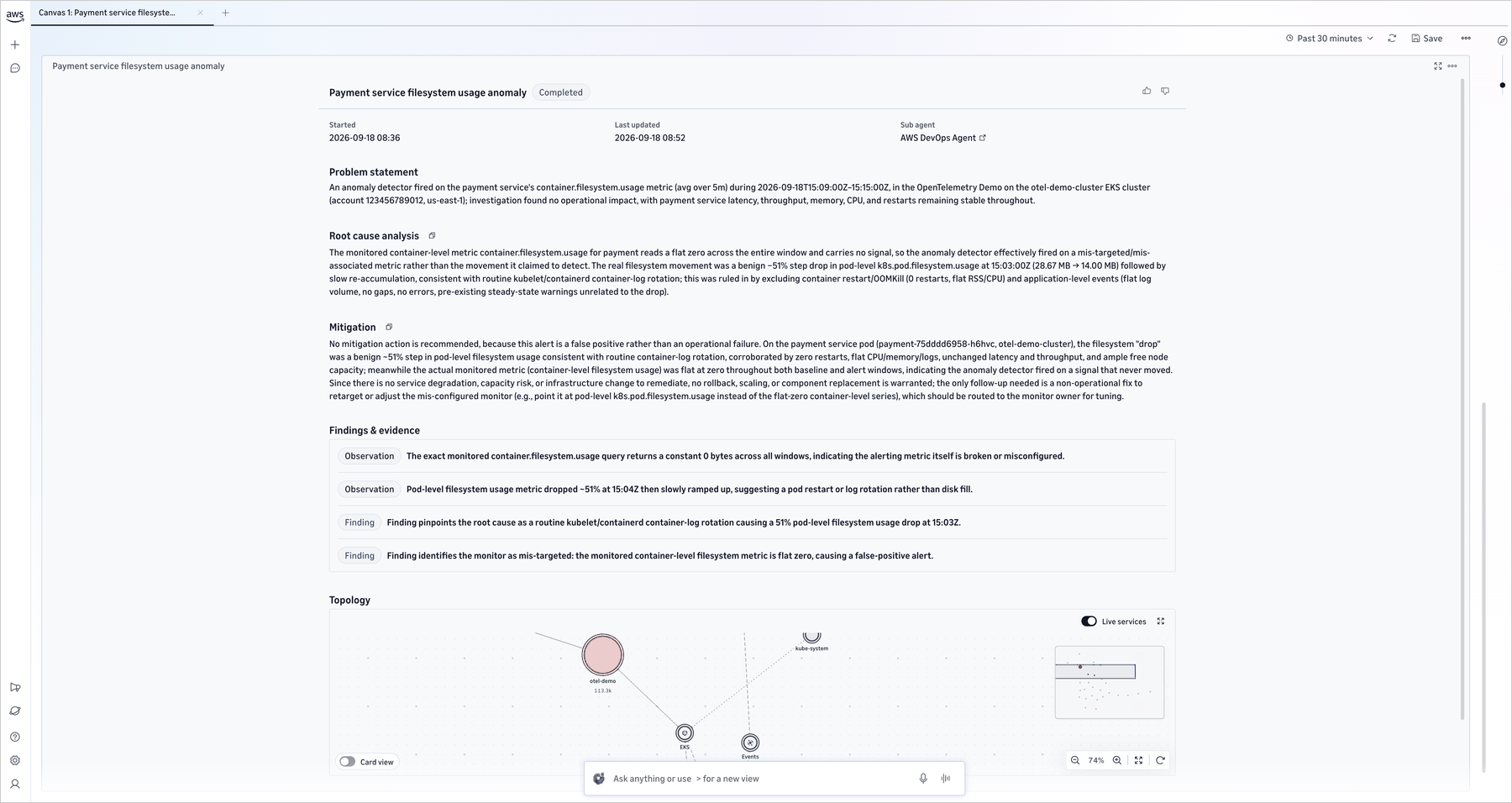
You can also set up service health alerts, configure what matters to your team, and trigger an AWS DevOps agent investigation to identify the root cause and develop a mitigation plan.


Figure 5. Investigation session — DevOps Agent identifies root causes and suggests next steps

Application-centric organization

CloudWatch Omni organizes telemetry by application rather than by infrastructure component. The system automatically discovers services from the telemetry data and AWS Config resource discovery, maps dependencies, and lets you see your application as a connected system rather than a collection of isolated resources.

Each team gets a Space that contains the applications they own. A Space points at existing CloudWatch data (logs, metrics, traces, and alarms) with no additional data movement required. Dynamic views replace the maintenance burden of static dashboards, providing ongoing visibility into SLOs and application health.

Getting started

Getting started takes minutes and doesn’t require reconfiguration of your existing CloudWatch setup.

If you’re an existing CloudWatch customer: Click “Try CloudWatch Omni” in the CloudWatch console. All your existing telemetry (logs, metrics, traces, and alarms) is immediately available. Workloads are discovered automatically, and you can start an investigation or browse your application topology right away.

For organization-wide deployment: An administrator configures a domain, connects your identity provider via IAM Identity Center, defines Spaces for teams and environments, and invites users. Each Space points at existing CloudWatch data with no additional data movement required.

For applications in other environments: CloudWatch Omni provides connectors that make it easy to bring in telemetry from additional environments. All ingested telemetry appears alongside your AWS data in the same Spaces and investigation sessions.

For generative AI and agentic workloads: The same CloudWatch Omni experience delivers purpose-built observability for AI agents, including trace exploration, evaluation frameworks, and real-time monitoring. In our companion post, we introduced the agent observability capabilities of Omni; for that walkthrough, see Introducing Amazon CloudWatch Omni: AI-powered observability for generative AI and agentic workloads.

Things to know

  • CloudWatch Omni extends CloudWatch. Existing alarms, dashboards, APIs, and console workflows continue unchanged.
  • Access is through a dedicated web application with enterprise SSO. Engineers don’t need AWS Console access to use it.
  • Once you setup, DevOps Agent is enabled by default in every Omni investigation session.

Pricing and availability

Amazon CloudWatch Omni is now available. Existing CloudWatch customers can try it directly from the CloudWatch console. For pricing details, visit the Amazon CloudWatch pricing page.

To get started, visit Amazon CloudWatch Omni or click “Try CloudWatch Omni” in the Amazon CloudWatch console.

If you want to call APIs, search documentation, find regional availability, and check troubleshooting about this feature, try using the AWS MCP Server and plugins with your preferred AI tool. Share your feedback on AWS re:Post or reach out through your usual AWS Support contacts.

— Daniel Abib

Introducing Amazon CloudWatch Omni: AI-powered observability for generative AI and agentic workloads

Post Syndicated from Daniel Abib original https://aws.amazon.com/blogs/aws/introducing-amazon-cloudwatch-omni-ai-powered-observability-for-generative-ai-and-agentic-workloads/

Today, Amazon CloudWatch introduces CloudWatch Omni, a unified observability experience for application and AI workloads that is app-centric, AI-powered, built on open standards, and delivered off-console. CloudWatch Omni is a purpose-built observability, evaluation, and experimentation solution for AI agents. It helps teams design, evaluate, and operate AI agents across any model provider, framework, or runtime, with an eval-driven workflow, support for the tools you already use, and observability delivered where you work: directly in your IDE and through a standalone web experience, separate from the AWS Management Console.

Organizations deploying agentic AI systems face observability challenges that traditional monitoring can’t address. Agent behavior is non-deterministic: a prompt change can degrade response quality even when standard metrics show no errors. Teams spend hours manually reviewing logs across multiple systems, unable to pinpoint what changed or why. Existing tools force teams to choose between siloed generative AI monitoring or fragmented solutions requiring constant context-switching between their coding environment and browser-based dashboards.

CloudWatch Omni captures every trace and includes built-in evaluators for correctness, coherence, retrieval quality, and tool selection, among others. You can compare prompt versions side by side in the playground, build test datasets from production traffic, run experiments across different configurations, and detect regressions automatically.

Two surfaces for development and operations

CloudWatch Omni delivers observability through two complementary surfaces. Developers get a native extension inside VS Code and Kiro (the currently supported IDEs), where traces appear as you run your agent with a playground and evaluators a click away. Operators get a standalone web experience, separate from the AWS Management Console to monitor the fleet, accessible through SSO with no AWS console needed. Both share the same data: the trace a developer debugs is the trace an operator investigates.

The Cloud Login feature connects your local IDE environment to your AWS account, enabling you to send telemetry data to Amazon CloudWatch for persistent storage, share traces with your team, and access production dashboards. This connection is optional. You can use CloudWatch Omni entirely locally during development, then connect to the cloud when you are ready to monitor agents in production.

Getting started

CloudWatch Omni offers two ways to get started: through the IDE extension (for VS Code and Kiro) or directly through the cloud experience, where you can start sending telemetry data to CloudWatch without installing any IDE extension. In this walkthrough, I install the extension, create an agent, run it, and explore the traces and evaluation tools from my IDE.

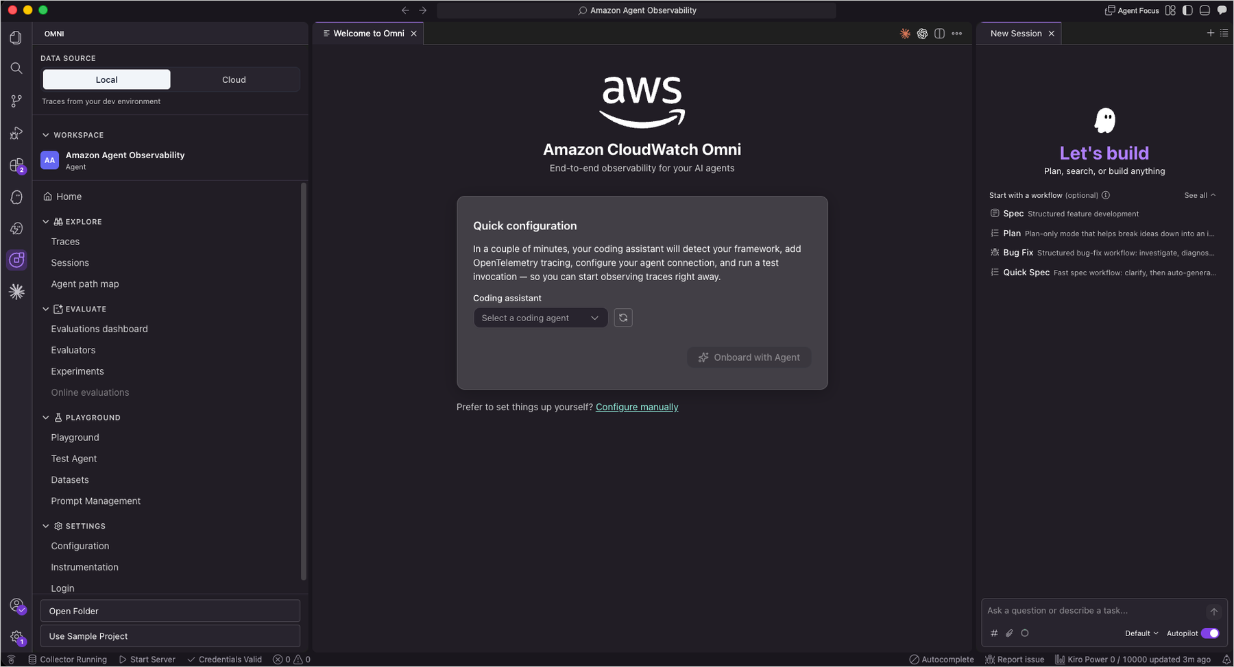
After installing the CloudWatch Omni extension from the VS Code Marketplace, the CloudWatch Omni icon appears in the Activity Bar. From the welcome screen, I selected Get started with Sample Project to load a pre-configured agent with sample trace data or use shortcut to Command Palette using Command + Shift + P (on macOS) or Ctrl + Shift + P (on Windows/Linux) and select Omni: Create a new Project

CloudWatch Omni welcome screen and create new project in VS Code

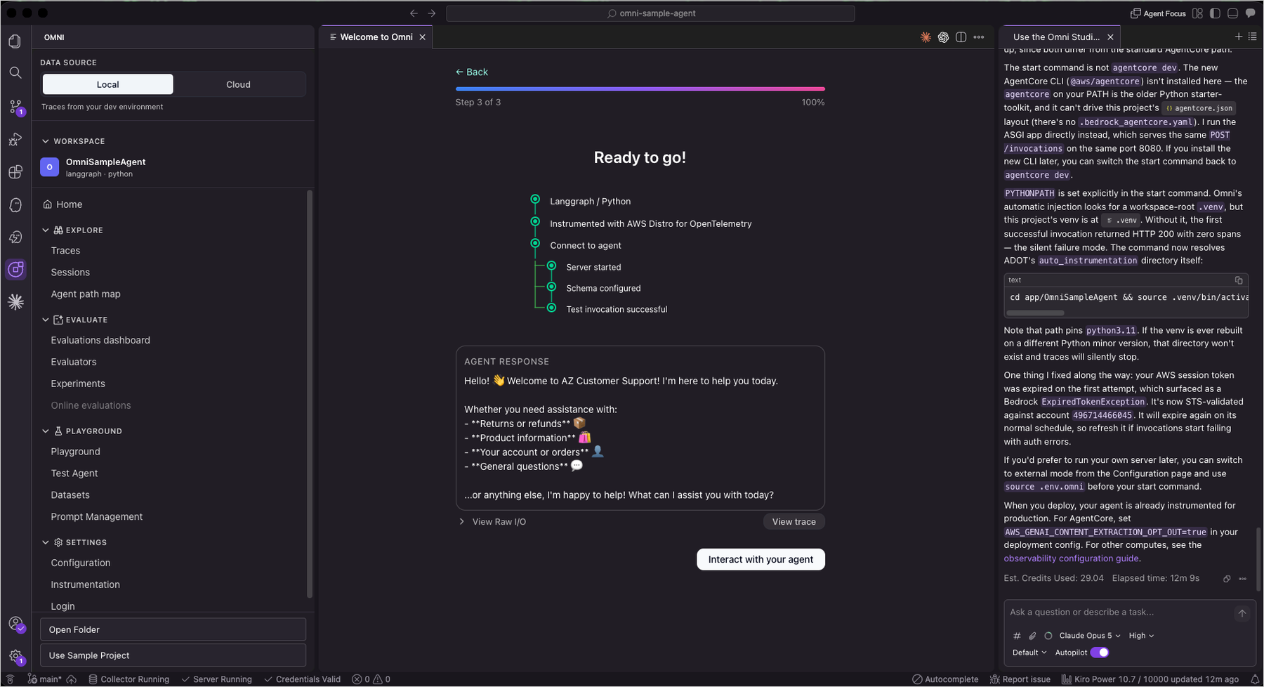
Figure 1. CloudWatch Omni welcome screen & create new project in VS Code

The sample project comes with an agent implementation and example datasets. Part of the getting-started experience is adding OpenTelemetry instrumentation, and CloudWatch Omni guides you through each step. You can also create a new agent from scratch. CloudWatch Omni walks you through the process using an interactive chat where you define the agent’s purpose, select a model provider, and configure tools. All data is stored locally by default. You can optionally connect to AWS to send data to Amazon CloudWatch.

After verifying the configuration, I started the local dev server and sent a question to the agent. What makes this different from a typical chatbot interface is what happens next: selecting View Trace shows exactly how the agent processed the request.

CloudWatch Omni guides your AI code assistant to configure the development environment

Figure 2. CloudWatch Omni guides your AI code assistant to configure the local development environment for testing

CloudWatch Omni integrates with AI code assistants such as Kiro, Claude Code, and Codex to streamline the setup process. These assistants can configure the Dev Server, install dependencies, and set up instrumentation on your behalf, so you can go from installation to running your first traced agent session in minutes without manual configuration.

Interacting with the agent and viewing traces

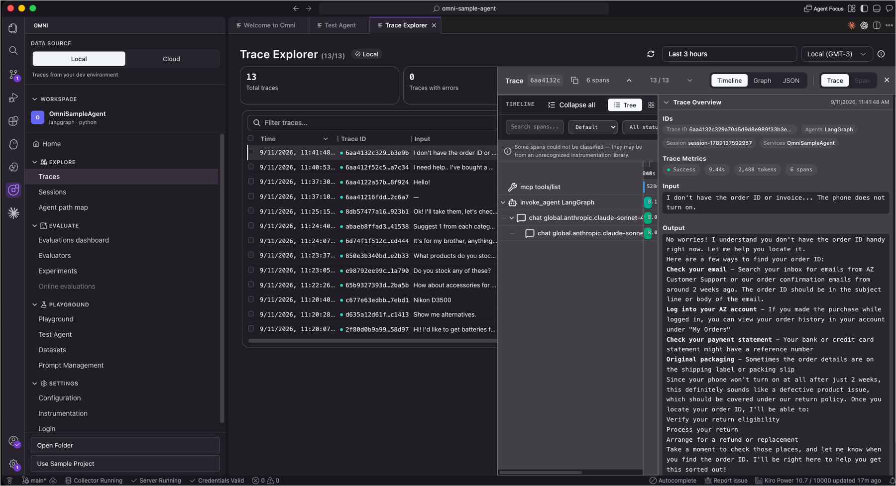
Figure 3. Interacting with the agent and viewing traces

Traces are essential for understanding AI agent behavior. Unlike traditional request-response systems, agents make multiple decisions per invocation: choosing tools, composing prompts, and chaining sub-calls. Without full trace visibility, diagnosing why an agent produced an incorrect answer or took an unexpected path becomes guesswork. CloudWatch Omni records every step in a structured timeline so you can pinpoint exactly where behavior diverged.

The Trace Explorer shows a detailed breakdown of every step the agent took (LLM calls, tool invocations, and reasoning steps) in a structured, hierarchical timeline. I could drill into any span to inspect inputs, outputs, token usage, and latency.

Trace Explorer showing the agent execution timeline

Figure 4. Trace Explorer showing the agent’s execution timeline

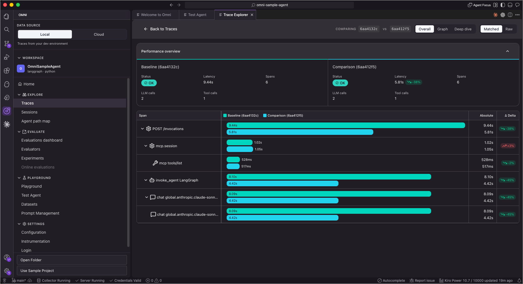
The Trace Explorer also supports Compare mode, which places two traces side by side to see how different prompts or configurations affect behavior. Compare mode is especially helpful when debugging regressions. And with Ask Assistant, an AI agent analyzes your traces to surface patterns and anomalies, answering questions like “Why did the agent call this tool twice?”

Comparing two traces side by side

Figure 5. Comparing two traces side by side

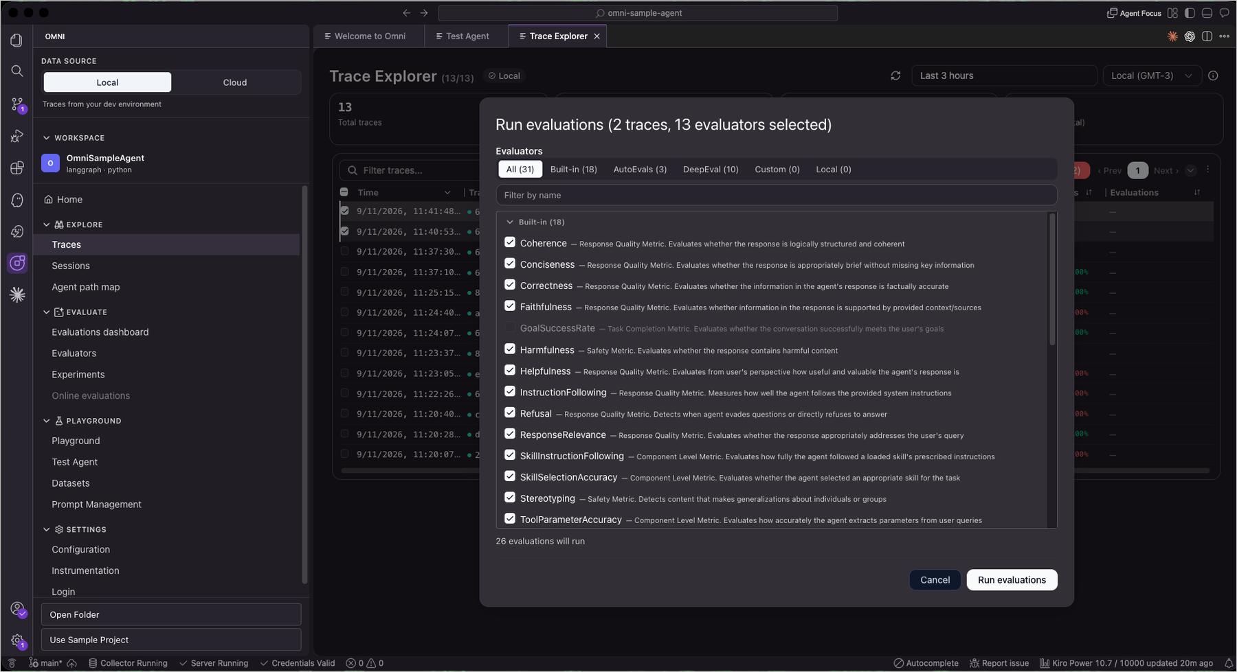
Evaluation is what turns observability into actionable quality improvement for generative AI. Traditional metrics like latency and error rate cannot tell you whether an agent’s response was helpful, coherent, or factually correct. Evaluators score each response against quality dimensions, letting you measure what users actually experience and catch regressions that standard monitoring misses entirely.

CloudWatch Omni includes 17 built-in evaluators for metrics like coherence, helpfulness, faithfulness, and routing correctness. I selected traces from the Trace Explorer, chose evaluators, and ran an evaluation, getting per-example scores and aggregate metrics without building any custom evaluation framework.

Running evaluations on traces

Figure 6. Running evaluations on traces

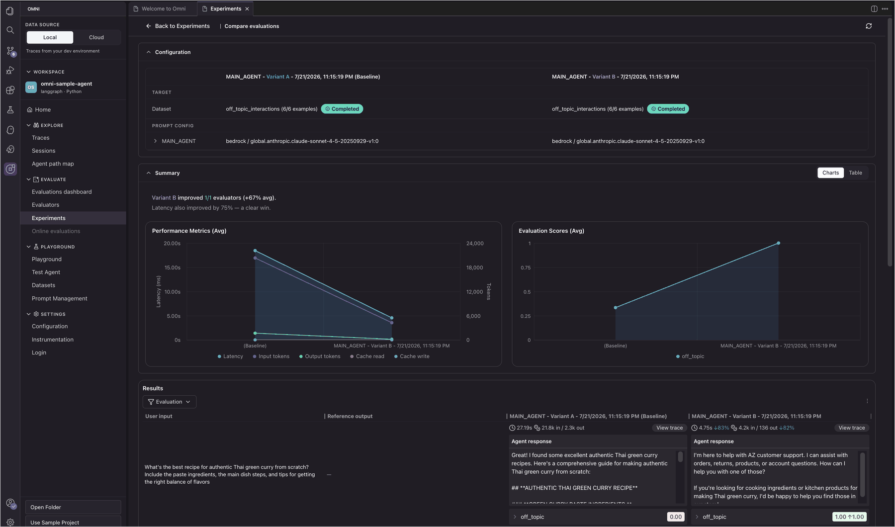
From there, I used the Playground to test different system prompts side by side, comparing multiple model and prompt configurations in real time to see how each variation affects output quality before committing changes. With the Experiments view, I could run the same dataset against two agent variants and compare their evaluation scores, latency, and token usage side by side to pick the best-performing configuration.

Figure 7. Comparing evaluations across agent variants in the Omni Experiments console

With Prompt Management, you can version and track prompt configurations over time, making it easy to roll back when a new version underperforms.

CloudWatch Omni also provides a Session Explorer to review full conversation histories and understand how agents handle multi-turn interactions, along with an Agent Topology view that visualizes the architecture of your agent system, including sub-agents, tools, and their interconnections. You can drill into any node to inspect performance and identify bottlenecks.

CloudWatch Omni also offers a dedicated web experience accessible from any browser without an IDE. Teams can access all capabilities collaboratively, including application monitoring, analytics, agent observability, and AI-powered investigations.

CloudWatch Omni web experience with application monitoring, analytics, and agent observability

Figure 8. CloudWatch Omni web experience with application monitoring, analytics, and agent observability

I curated traces into golden datasets for structured experimentation. The Experiment function runs the agent against a dataset and automatically scores results, creating benchmarks for regression testing whenever prompts or agent logic change.

If you already have an agent built with a supported framework, CloudWatch Omni provides two paths to add instrumentation: Auto-instrument with Kiro, which detects your framework and configures tracing automatically, or manual instrumentation with ready-to-use code snippets for Python and TypeScript. For detailed instrumentation guides, see the CloudWatch Omni documentation.

Supported frameworks and open standards

The walkthrough above uses the sample project, but CloudWatch Omni works with the agent frameworks teams are already using: LangChain, LangGraph, CrewAI, OpenAI SDK, Strands, Vercel AI SDK, and more, in both Python and TypeScript. It also provides native observability for agents built with Amazon Bedrock AgentCore, and uses AgentCore’s evaluation capabilities to assess agent quality directly within the Omni workflow.

Instrumentation uses open standards (OpenInference and ADOT), whether your agents run on Lambda, ECS, EKS, or other clouds. For evaluation, Omni integrates with third-party evaluators including Braintrust, DeepEval, and Ragas, alongside built-in datasets, a playground, and batch experiments. No re-platforming required.

CloudWatch Omni brings agent observability and application observability together in a single experience. For the application observability experience, read the companion post Introducing Amazon CloudWatch Omni: collaborative AI-powered observability for your applications.

Pricing and availability

Amazon CloudWatch Omni is now generally available. The IDE extension is free to use. You don’t need an AWS account to get started. You only need AWS credentials for Amazon Bedrock models, or API keys for other providers like OpenAI or Anthropic. Get started today by installing the extension from the VS Code Marketplace.

To explore all capabilities and get started quickly, visit CloudWatch on AWS Builder Center.

If you want to call APIs, search documentation, find regional availability, and check troubleshooting about this feature, try using the AWS MCP Server and plugins with your preferred AI tool. Share your feedback on AWS re:Post or reach out through your usual AWS Support contacts.

Happy building!

— Daniel Abib

New low-cost burstable Amazon EC2 T8i instances are generally available

Post Syndicated from Channy Yun (윤석찬) original https://aws.amazon.com/blogs/aws/new-low-cost-burstable-amazon-ec2-t8i-instances-are-generally-available/

Today, we’re announcing the general availability of new low-cost burstable Amazon EC2 T8i instances powered by custom sixth generation Intel Xeon Scalable Processors (Granite Rapids), available only on AWS. T8i instances are among the lowest-cost EC2 instances and deliver up to 30% better price performance over previous generation T3 instances. These instances are designed to run a variety of low-to-moderate CPU utilization workloads such as freemium services, training and demo environments, staging and development, data processing, microservices, low-traffic websites, and login gateways.

T8i instances
Thousands and thousands of customers run various lightweight workloads on T3 instances that require small, cost-effective compute configurations. These include microservices architectures, low-traffic websites, development and testing environments, small databases, data processing jobs, and short-duration compute tasks. Many of these customers like T family’s burstable performance model, which provides a baseline level of CPU performance with the ability to burst above the baseline when needed using CPU credits.

As customers modernize their infrastructure, migrate from on-premises environments, adopt event-driven and microservices architectures, and experiment with AI inference workloads, they have asked for newer generation cost-optimized small instances, better price performance to reduce their total cost of ownership, and a seamless migration path that leverages their existing knowledge and tooling.

T8i instances address each of these requests:

  • Up to 30% better price performance. Powered by the AWS Nitro System and custom sixth generation Intel Xeon Scalable Processors (Granite Rapids), T8i instances enable customers to lower their total cost of ownership with up to 30% better price performance.
  • Up to 70% higher compute performance. T8i instances deliver up to 70% higher compute performance, up to 1.25x higher network bandwidth, and up to 2.4x higher EBS bandwidth compared to T3 instances.
  • Seamless upgrade from T3. For existing T3 customers, upgrading to T8i is straightforward. The instances offer the same CPU credit system and the same familiar lightweight compute options customers already know. Customers simply select T8i instead of T3 and immediately benefit from improved price performance.
  • Cost-effective entry point for new customers. For customers new to AWS or migrating from on-premises, T8i instances provide one of the most cost-effective entry points to run workloads that need low-to-moderate CPU utilization or for running short-duration compute tasks such as batch processing, event-driven functions, or CI/CD pipelines.

Instance specifications
T8i instances offer four sizes, each with two vCPU offered as a single core. The following table summarizes the specifications.

Instance size vCPUs Memory (GiB) Baseline Performance /vCPU (%) CPU credits earned / hour Network burst bandwidth (Gbps)
t8i.nano 2 0.25 5 3 Up to 6.25
t8i.micro 2 0.5 10 6 Up to 6.25
t8i.small 2 1 20 12 Up to 6.25
t8i.medium 2 2 20 12 Up to 6.25

Like T3, T8i instances offer unique vCPU-to-memory ratios such as 1:0.25, 1:0.5, and 1:1 that are not offered by other EC2 instances. Like T3, T8i instances utilize the CPU credit system along with the Standard and Unlimited credit configuration modes. Unlimited mode is the default on T8i.

For workloads that need larger instance sizes above T8i offerings (nano, micro, small, and medium), I recommend M8i Flex instances that offer up to 30% better price performance than equivalent previous generation T3 instances along with the flexibility to scale up to 16xlarge.

Now available
Amazon EC2 T8i instances are available today in the following AWS Regions: US East (N. Virginia, Ohio), US West (Oregon, N. California), Asia Pacific (Hyderabad, Malaysia, Mumbai, Seoul, Singapore, Sydney, Tokyo), Canada (Central), and Europe (Frankfurt, Ireland, London, Paris). For Regional availability and upcoming Region expansion, search the instance type in the CloudFormation resources tab of AWS Capabilities by Region.

You can purchase T8i instances via On-Demand instances, and Spot instances with Savings Plan option coming soon. T8i instances support shared tenancy only and do not support Dedicated tenancy or Dedicated Hosts. t8i.micro and t8i.small instances are also available under the AWS Free Tier. To learn more, visit the Amazon EC2 Pricing page.

Try T8i instances in the Amazon EC2 console and send feedback to AWS re:Post for EC2 or through your usual AWS Support contacts.

— Channy
AWS Elastic Beanstalk introduces Cluster Mode

Post Syndicated from Channy Yun (윤석찬) original https://aws.amazon.com/blogs/aws/aws-elastic-beanstalk-introduces-cluster-mode/

Since the first launch of AWS Elastic Beanstalk in 2011, customers have deployed full-stack applications in Java, .NET, Python, Node.js, PHP, Ruby, and Go, trusting Elastic Beanstalk to manage deployment and infrastructure operations so they could focus on business logic. Fifteen years later, that trust has only deepened, and the service has been rebuilt to match it. Now, AWS Elastic Beanstalk is the application management service on AWS that takes full operational responsibility for your production environments. Bring applications however they exist today: source code, Dockerfiles, or container images. Elastic Beanstalk creates and manages the production environment underneath. You manage your application. AWS manages everything else, deploying, scaling, patching, monitoring, and maintaining it continuously. That operational responsibility stays with AWS, for the life of the application.

We have been rebuilding the operational engine underneath and delivering a series of capabilities that make it more powerful than ever. Elastic Beanstalk now uses AI-powered environment analysis to diagnose health issues and recommend fixes automatically. A new official GitHub Action lets teams deploy directly from their existing CI/CD workflows with a single YAML configuration. And we rebuilt the infrastructure foundation to deliver OpenTelemetry-based observability, traffic-splitting deployments with automatic rollback, event-driven autoscaling, secrets management through AWS Secrets Manager, and HTTPS by default via AWS Certificate Manager.

Today, we’re announcing the next chapter of AWS Elastic Beanstalk: a new fully-managed Cluster Mode that deploys, scales, patches, monitors, and upgrades your applications continuously for the life of the workload. You bring your application. AWS runs it.

A new Cluster Mode is built for teams running a portfolio of applications. Instead of operating each application in isolation, you run multiple applications that share infrastructure powered by Amazon Elastic Kubernetes Service (Amazon EKS), fully managed with a single operational baseline. Multiple applications share resources, so per-application cost decreases as your portfolio grows without adding operational complexity. Whether you run ten applications or a hundred, you manage them through one experience, with the same operational guarantees across every stack.

Elastic Beanstalk Cluster Mode benefits for your workloads:

  • Source code to production, any runtime. Upload source code in Java, .NET, Python, Node.js, PHP, Ruby, or Go. Elastic Beanstalk handles containerization automatically through Cloud Native Buildpacks when needed. No Dockerfile and no rearchitecting required. You can bring legacy applications from on-premises or deploy new services in any supported language.
  • Enterprise compliance built in. Elastic Beanstalk is HIPAA eligible, PCI DSS compliant, and aligned to SOC 1/2/3 with no additional configuration, so teams in regulated industries can deploy production workloads with the compliance posture they already require.
  • Production-grade deployment strategies. All-at-once, rolling, immutable, and traffic-splitting deployments with automatic rollback on failure. Event-driven autoscaling. AWS Secrets Manager integration. All native OpenTelemetry enabling easy integration with most observability backends, including Amazon CloudWatch.
  • AI-powered troubleshooting. When something goes wrong, Elastic Beanstalk collects service-side logs and provides AI-generated recommendations to help you resolve issues faster without digging through infrastructure.

A first look of Elastic Beanstalk Cluster Mode
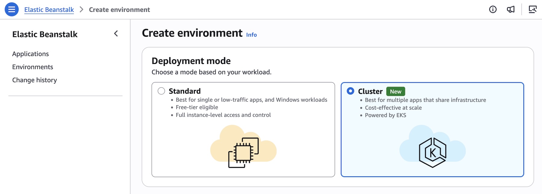
To get started, go to the Elastic Beanstalk console, create a new environment, and choose the Cluster in the Deployment type.

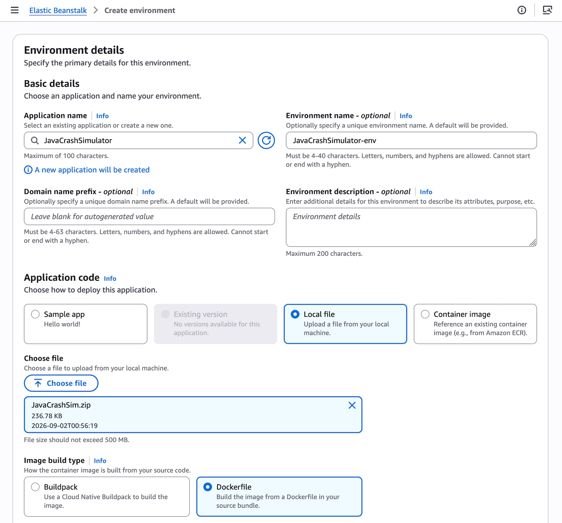
Elastic Beanstalk accepts source code, docker file, or container image to deploy your application. For example, you can provide the application code for your environment by selecting Local file and specifying container image build options. For the rest of the sections, the default values should be good for most scenarios.

Choose Create button and the deployment will begin! Note that the first deployment for a given set of subnets triggers EKS cluster creation, which takes about ten-ish minutes. Subsequent deployments are faster because they reuse an existing EKS cluster.

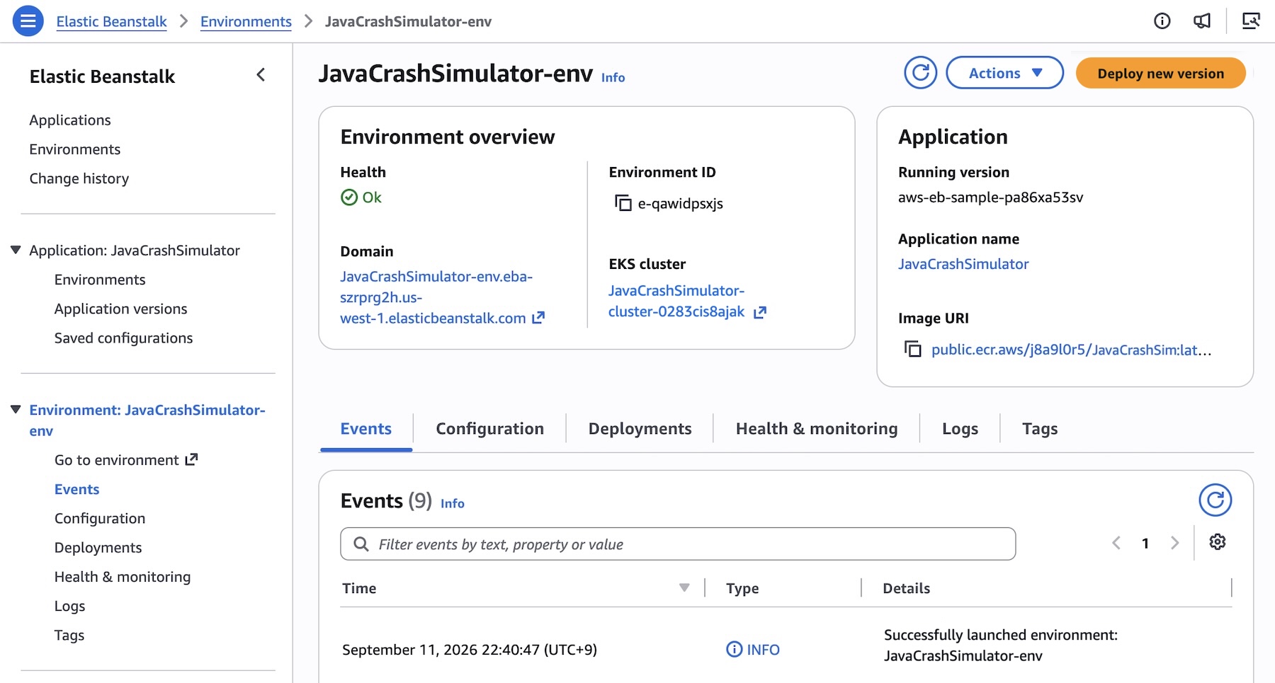
Here’s what it looks like when deployment is successful:

You can also use AWS Command Line Interface (AWS CLI), the EB CLI, or AWS SDKs. For example, consider deploying an application made up of several microservices to Kubernetes. Create an application first.

aws elasticbeanstalk create-application \
    --application-name "my-microservice" \
    --description "Multi-services demo" \

Each microservice may have pre-built images in Amazon Elastic Container Registry (Amazon ECR). Register them as application versions:

IMAGES=(
    "frontend-v1|public.ecr.aws/my-microservices/frontend:v1"
    "cartservice-v1|public.ecr.aws/my-microservices/cart:v1"
    "paymentservice-v1|public.ecr.aws/my-microservices/payment:v1"
    "shippingservice-v1|public.ecr.aws/my-microservices/shipping:v1"
)

for entry in "${IMAGES[@]}"; do
    IFS='|' read -r label uri <<< "$entry"
    aws elasticbeanstalk create-application-version \
        --application-name $APP_NAME \
        --version-label "$label" \
        --image-configuration Source="{Uri=$uri}" \
	--region "us-west-2
    echo "Registered: $label"
done

You can set and deploy the corresponding service options for each service. For example, the frontend service is the only service that needs a public internet interface such as Application Load Balancer and also sets a health check path since it’s an HTTP service:

[
    {"Namespace": "aws:elasticbeanstalk:eks", "OptionName": "cluster-role", "Value": "arn:aws:iam::0123456789012:rol<...>"},
    {"Namespace": "aws:elasticbeanstalk:eks", "OptionName": "node-role", "Value": "arn:aws:iam::0123456789012:role/E<...>"},
    {"Namespace": "aws:elasticbeanstalk:eks:environment", "OptionName": "observability-role", "Value": "arn:aws:iam::0123456<...>"},
    {"Namespace": "aws:elasticbeanstalk:eks:environment", "OptionName": "subnets", "Value": "subnet-1,subnet-2,subnet-3,<...>"},
    {"Namespace": "aws:elasticbeanstalk:eks:environment:autoscaling", "OptionName": "min-replica", "Value": "1"},
    {"Namespace": "aws:elasticbeanstalk:eks:environment:autoscaling", "OptionName": "max-replica", "Value": "2"},
    {"Namespace": "aws:elasticbeanstalk:eks:environment", "OptionName": "cpu", "Value": "0.5"},
    {"Namespace": "aws:elasticbeanstalk:eks:environment", "OptionName": "memory", "Value": "256Mi"},
    {"Namespace": "aws:elasticbeanstalk:eks:environment", "OptionName": "memory-limit", "Value": "512Mi"},
    {"Namespace": "aws:elasticbeanstalk:eks:environment", "OptionName": "service-port", "Value": "8080"},
    {"Namespace": "aws:elasticbeanstalk:eks:alb", "OptionName": "scheme", "Value": "internet-facing"},
    {"Namespace": "aws:elasticbeanstalk:eks:alb", "OptionName": "healthcheck-path", "Value": "/_healthz"}
] #frontend-options.json namespaces

Now, create the frontend service environment with these options. You can continue to deploy each service environment in a similar manner.

aws elasticbeanstalk create-environment \
    --application-name my-microservice \
    --environment-name frontend \
    --version-label frontend-v1 \
    --tier Name=Cluster,Type=EKS \
    --option-settings file:///tmp/frontend-options.json \

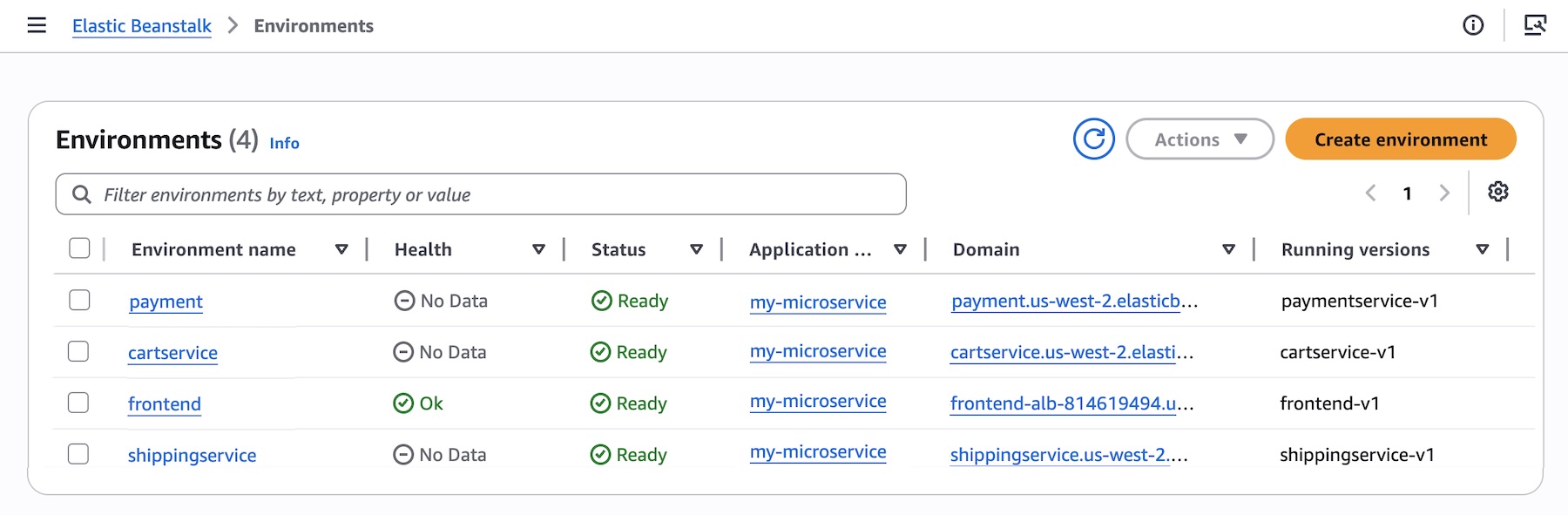
Here’s a look at the console once all services are deployed:

Elastic Beanstalk Standard powered by Amazon Elastic Compute Cloud (EC2) continues to be fully supported. Standard and Cluster Mode environments run side by side within the same Elastic Beanstalk application, enabling teams to migrate one environment at a time at their own pace. Validation checks confirm compatibility before any changes are made, so no environment is forced to move.

Elastic Beanstalk Standard Mode remains the best fit for:

  • Single applications or single-environment use cases
  • Windows/.NET Framework workloads on IIS
  • Applications that cannot be containerized
  • Workloads spending under $500/month where the EKS control plane fee and EKS Auto Mode premium add overhead that a single application cannot offset through bin-packing

To learn more about how to deploy and manage your applications in the Cluster Mode, visit the Elastic Beanstalk Cluster Mode documentation.

Now available
AWS Elastic Beanstalk Cluster Mode is generally available today in all AWS Regions that Elastic Beanstalk is available. For Regional availability and a future roadmap, visit the AWS Capabilities by Region. If you want to call APIs, search documentation, find regional availability, and troubleshooting about this new feature, try using the AWS MCP Server and plugins with your preferred AI tool.

There is no additional charge for Elastic Beanstalk Cluster Mode. You pay only for the underlying AWS resources your applications consume, including the EKS control plane fee, EKS Auto Mode compute (approximately 12% premium on EC2 instance costs), Amazon ECR, and Amazon CloudWatch. Note Elastic Beanstalk Cluster Mode is not AWS Free Tier eligible. To learn more, visit the AWS Elastic Beanstalk Pricing page.

Give it a try in the Elastic Beanstalk console and send feedback to AWS re:Post for AWS Elastic Beanstalk or through your usual AWS Support contacts.

— Channy

AWS reimagines the getting started experience

Post Syndicated from Micah Walter original https://aws.amazon.com/blogs/aws/aws-reimagines-the-getting-started-experience/

Amazon Web Services (AWS) started with a handful of foundational infrastructure services such as Amazon Simple Storage Service (Amazon S3), Amazon Elastic Compute Cloud (Amazon EC2), and Amazon Simple Queue Service (Amazon SQS), so that anyone with an idea could start building. As the world’s largest companies and governments adopted AWS, they asked for features to optimize their configuration for a range of global business contexts, security requirements, and operational needs. To meet these needs, AWS expanded globally through new Regions and added breadth and depth of services in security, networking, governance, and cost controls, so those customers could operate wherever they needed and at the scale they require. That combination of global reach, breadth, and depth remains essential for those customers, but if you are at the start of a new idea, every configuration option is effort standing in the way of shipping your dream product fast.

Today, we’re announcing a new simplified experience on AWS for builders who are working at the pace of AI. Instead of having to complete configuration tasks before you can work on your project, you start with sensible defaults and simple administration. You sign up using an existing identity from providers including Google, GitHub, and Apple. For most new customers, no credit card is required to start and you receive $100 in free credits as part of the AWS Free Tier. You can build immediately in your first project. As you continue to work, you can invite collaborators with just an email address, without learning about AWS Identity and Access Management (IAM) or AWS IAM Identity Center. When your project grows beyond the free credits, you can set a spend limit so you stay within your budget on the paid plan. If you grow to need additional customization, you can activate advanced AWS features to access the full breadth and depth of AWS without migrating.

How it works
When you sign up, AWS organizes your work in a project. A project contains an AWS account, where you create resources, and settings for sharing with team members. AWS creates that structure for you and applies additional security controls so you can start building your idea. After signing in, you get a prompt to paste into your coding agent that configures it to work with your new AWS environment. From there, your agent can deploy resources, run workloads, and iterate on your application following best practices for working with AWS.

You can create another project with a click. When you want to work with an additional team member, you send an invitation to their email address. Identity permissions are handled for you, so there are no IAM users to create; each person you invite only gets access to the projects you specify. Console workflows and coding agents also configure permissions between supported services and resources automatically, so you do not have to set up or troubleshoot resource permissions by hand.

When you’re ready to move beyond free credits, you can upgrade to a paid plan by entering your payment method. You can set a monthly spend limit on a project based on your usage trends, starting at $20 per month. The spend limit is the ceiling for that project’s costs, and you pay for what you actually use up to that amount. For example, if you set a $50 spend limit and your project incurs $32 in charges that month, you pay $32 (plus taxes). AWS will suggest a spend limit based on your usage, and you can accept that recommendation or set a custom amount if you are planning to further scale your usage. If your project approaches the limit, you first receive notifications. If spend reaches the limit, AWS pauses your project rather than accumulating charges, and you can resume working on it when you raise the limit. Each project has its own spend limit so you can give a larger budget to a workload that is gaining traction while keeping a smaller budget on an experimental idea.

Let’s try it out
To get started, I went to aws.amazon.com and chose Create account. I signed in with my Google account and within seconds had a new project ready to go, as shown in the following screenshot.

The Sign up for AWS page, with options to continue with email or sign in using Google, GitHub, Apple, or Amazon.

The first thing I saw was a prompt to configure my coding agent. I copied the prompt and pasted it into my agent. The agent set up the AWS Command Line Interface (AWS CLI) and the Agent Toolkit for AWS, logged me into AWS, and created a CLAUDE.md file in my project with guidance for the new experience.

The Setup Agent Toolkit for AWS dialog, with a prompt to copy and paste into your coding agent.

With the agent connected, I gave it a short prompt: build an API that returns a new unique sequential ID on every request. The agent created an AWS Lambda function, an Amazon DynamoDB table, and an Amazon API Gateway API, then deployed them for me. I did not have to configure resource permissions by hand. Within a few minutes I had a public endpoint that returned a newly minted ID on each request. My project started with $100 in free credits, and I received an additional $20 when the Lambda function was deployed.

A coding agent prompt to build an API that returns a unique sequential ID on every request.

The coding agent presents architecture options for the sequential ID API, with AWS Lambda and Amazon DynamoDB selected.

The coding agent confirms the API is live and lists the Amazon DynamoDB table, AWS Lambda function, and Amazon API Gateway API it deployed.

From the project, I could manage settings, invite team members by email, and monitor billing, as shown in the following screenshots.

The Projects page, showing remaining free-plan days, credits, and a project.

The project Members page, with the option to invite a new team member by email.

The Billing page, showing a $0.00 balance on the free plan, remaining credits, and cost by project.

Activating advanced features
If you reach the point where you need multiple Regions, or governance features like custom policies in AWS Organizations, you can activate advanced features at no additional cost. You’ll find yourself in a fully configured AWS Organization built according to best practices, with no migration and no downtime. Everything you configured previously is preserved and reflected in the underlying AWS services.

Now rolling out
We’ve heard from builders that they do not want to spend their first hours configuring an AWS environment. They want to build what they came to build, and we listened. AWS began as a place where anyone with an idea could start building, and this new simplified experience brings that starting point back, with sensible defaults so you can begin immediately, and with the global reach, breadth, and depth of AWS still there when your idea needs it. We are gradually rolling this experience out to new customers. We cannot wait to see what you build, and we want your feedback on the experience.

To try the new experience, create a new AWS account. To learn more, see Sign up for AWS (new).

Introducing Amazon EBS Volume Clones across AWS accounts

Post Syndicated from Channy Yun (윤석찬) original https://aws.amazon.com/blogs/aws/introducing-amazon-ebs-volume-clones-across-aws-accounts/

Last year, we introduced Volume Clones of Amazon Elastic Block Store (Amazon EBS), a new capability that lets you create instant point-in-time copies of your EBS volumes within the same Availability Zone.

Today, we are extending Volume Clones with cross-account copy, so you can create copies of your EBS volumes into other AWS accounts and optionally re-encrypt them with an AWS Key Management Service (AWS KMS) key in the target account.

With this new feature, you can use your latest application data to develop, test, and experiment in a secondary environment, while protecting and isolating the information in the production environment. For example, you can create copies of a production environment to refresh test and development environments set up in separate accounts with the desired EBS encryption.

Copy EBS volumes across AWS accounts in action
To create a copy of an EBS volume across accounts, the owners of the volume can first grant the target account access to their volume in AWS Resource Access Manager (RAM), which provides a way to share resources across AWS accounts or within an AWS Organization. Then, from the target account, they can locate the volume they have access to create a copy of it.

To get started, choose Share volume for the volume you want to share with the target account in the Amazon EBS console.

Share the volume with other AWS accounts by adding it to existing resource shares, or create a new resource share in the AWS RAM console. For more details, refer to the AWS RAM User Guide.

You can now see confirmation that the volume has been shared in the Volume sharing tab of the volume detail page.

A target account must accept the resource share on the RAM console.

Once they accept the resource share, they can see the volumes in the EBS volume page of the target account. Choose Copy volume for any shared volume.

To share and copy EBS volumes across AWS accounts programmatically, including calling APIs and searching documentation, try the AWS MCP Server and plugins with your preferred AI coding tool. To learn more, visit the Amazon EBS User Guide.

Things to know
Let me share some important technical details that I think you’ll find useful.

  • Encryption: You can share unencrypted volumes and volumes encrypted with a customer managed key (CMK). Volumes encrypted with the default AWS managed key (AMK) cannot be shared. When copying a shared volume encrypted with a CMK, the CMK must also be shared with the target account. You can specify a different CMK to re-encrypt the copy in the target account.
  • Monitoring: You can monitor SharedVolumeCopyInitiated through AWS CloudTrail event in your account. You will also receive events in Amazon EventBridge at the start of the copy operation when the state of the copied volume is initializing, and at the end of the operation when the state of the copied volume changes to completed. You can see the shared volume ID, consuming account ID, and event time.
  • Pricing: Once a copy is initiated, you’ll pay a one-time fee based on your volume size, charged to the account where the copy will reside. There’s no cost for sharing EBS volumes through AWS RAM. The copied volume will incur regular EBS volume charges upon creation.
  • Availability Zone: The volume copy must be created in the same Availability Zone as the source volume. Use Availability Zone IDs (such as use1-az1) to identify the same physical location across accounts.

Now available
Cross-account volume clones for Amazon EBS are available in all AWS Regions that support Amazon EBS Volume Clones. For Regional availability and a future roadmap, visit the AWS Capabilities by Region.

Give this feature a try in the Amazon EC2 console today and send feedback to AWS re:Post for Amazon EBS or through your usual AWS Support contacts.

— Channy

Amazon EC2 R9g and R9gd instances powered by AWS Graviton5 processors are now generally available

Post Syndicated from Daniel Abib original https://aws.amazon.com/blogs/aws/amazon-ec2-r9g-and-r9gd-instances-powered-by-aws-graviton5-processors-are-now-generally-available/

Today, Amazon EC2 R9g and R9gd instances are generally available, powered by AWS Graviton5 processors. R9g instances are memory-optimized and deliver up to 25% better compute performance compared to Graviton4-based R8g instances, powered by the most energy efficient processor AWS has ever built.

R9g instances are ideal for memory-intensive workloads including databases, in-memory caches (Valkey, Redis, MemCached), real-time big data analytics, Linux-based workloads including containerized and micro-service-based applications (e.g. Kubernetes, Docker, EKS, ECS), as well as applications written in popular programming languages such as C/C++, Rust, Go, Java, Python, .NET Core, Node.js, Ruby, and PHP.

R9gd instances include local NVMe-based SSD block-level storage, ideal for memory-intensive workloads requiring fast, low-latency local storage such as open-source databases, distributed real-time big data analytics, large in-memory databases, and large caching workloads.

If you’re running workloads on R8g instances today, R9g gives you more performance per vCPU with faster memory, higher network and Amazon EBS bandwidth, and a larger L3 cache, all while using less energy.

What makes R9g different
Graviton5 processors bring several hardware improvements over Graviton4:

  • Up to 25% higher compute performance per vCPU
  • DDR5 8800 MT/s memory (up from 5600 MT/s in Graviton4), the fastest memory available in the cloud
  • 5x larger L3 cache for better data locality
  • Up to 2x higher network and EBS bandwidth for the largest instance sizes (up to 100 Gbps network, up to 72 Gbps EBS on the 48xlarge)
  • Up to 3x higher packet-processing performance

R9g and R9gd instances support Instance Bandwidth Configuration (IBC), which lets you adjust the allocation of bandwidth between Amazon EBS and Amazon VPC networking by 25%. This helps optimize performance for workloads with specific bandwidth requirements such as databases and caching.

All R9g and R9gd instances run on the AWS Nitro System, which offloads virtualization, storage, and networking to dedicated hardware. This gives your applications near-bare-metal performance while maintaining strong security isolation between instances.

R9g and R9gd instances feature the Nitro Isolation Engine (NIE), the same enhancement to the Nitro System introduced with C9g and M9g instances earlier this year, which enforces isolation of instances and harnesses formal verification to provide assurances of isolation with mathematical precision. Nitro Isolation Engine is a purpose-built component that is responsible for enforcing isolation between virtual machines, including mediation of all access to virtual machine memory, CPU register state, and I/O devices through a minimal set of APIs. Nitro Isolation Engine leverages formal verification, a technique to mathematically demonstrate that the hardware or software behaves as intended, and not just in specific test cases. This intensive verification technique establishes Nitro as the first formally verified cloud hypervisor, pioneering a new standard for mathematically proven cloud security. To learn more about the Nitro Isolation Engine, visit the blog post. For details on the formal verification results, including scope and assumptions, see the technical white paper.

EC2 R9g and R9gd instance specifications
R9g and R9gd instances are each available in 11 sizes, from medium to metal-48xl. The following tables show the full specifications for each size.

Instance size vCPUs Memory (GiB) Instance Storage Network Bandwidth (Gbps) EBS Bandwidth (Gbps)
r9g.medium 1 8 EBS-Only Up to 15 Up to 12
r9g.large 2 16 EBS-Only Up to 15 Up to 12
r9g.xlarge 4 32 EBS-Only Up to 15 Up to 12
r9g.2xlarge 8 64 EBS-Only Up to 17 Up to 12
r9g.4xlarge 16 128 EBS-Only Up to 17 Up to 12
r9g.8xlarge 32 256 EBS-Only 17 12
r9g.12xlarge 48 384 EBS-Only 25 18
r9g.16xlarge 64 512 EBS-Only 34 24
r9g.24xlarge 96 768 EBS-Only 50 36
r9g.48xlarge 192 1536 EBS-Only 100 72
r9g.metal‑48xl 192 1536 EBS-Only 100 72

R9gd instances offer the same compute and networking performance as R9g, with the addition of local NVMe-based SSD storage for workloads that need fast, low-latency scratch space or temporary caches.

Instance size vCPUs Memory (GiB) Instance Storage (NVMe SSD) Network Bandwidth (Gbps) EBS Bandwidth (Gbps)
r9gd.medium 1 8 1 x 59 GB Up to 15 Up to 12
r9gd.large 2 16 1 x 118 GB Up to 15 Up to 12
r9gd.xlarge 4 32 1 x 237 GB Up to 15 Up to 12
r9gd.2xlarge 8 64 1 x 474 GB Up to 17 Up to 12
r9gd.4xlarge 16 128 1 x 950 GB Up to 17 Up to 12
r9gd.8xlarge 32 256 1 x 1900 GB 17 12
r9gd.12xlarge 48 384 3 x 950 GB 25 18
r9gd.16xlarge 64 512 1 x 3800 GB 34 24
r9gd.24xlarge 96 768 3 x 1900 GB 50 36
r9gd.48xlarge 192 1536 3 x 3800 GB 100 72
r9gd.metal‑48xl 192 1536 3 x 3800 GB 100 72

Getting started
You can launch R9g and R9gd instances from the Amazon EC2 console using any supported Arm-based AMI. R9g instances support Amazon Linux 2023, Amazon Linux 2, Ubuntu 22.04+, RHEL 8.4+, SUSE Linux Enterprise Server 15 SP3+, Debian 12+, and other major Linux distributions.

If you’re migrating from R8g, no code changes are required for most applications. Select the equivalent R9g instance size and your application runs with better performance. For containerized workloads, R9g works with Amazon EKS, Amazon ECS, and standard Kubernetes deployments. Multi-arch container images built for Arm64 run without changes.

Several resources help you get started: the AWS Graviton Getting Started Guide covers how to build, run, and optimize workloads on Graviton-based instances. The Graviton Savings Dashboard helps you track cost savings. AWS Transform automates code transformations for migrating Java applications from x86 to Graviton. To learn more, visit AWS Graviton Processors or Level up your compute with AWS Graviton.

Pricing and availability
Amazon EC2 R9g and R9gd instances are available in US East (N. Virginia, Ohio), US West (Oregon), and Europe (Frankfurt) Regions.

R9g and R9gd instances are available for purchase through Savings Plans, On-Demand, Spot Instances, Dedicated Instances, or Dedicated Hosts. For detailed pricing, visit the Amazon EC2 pricing page.

Ready to get started? Launch R9g instances from the Amazon EC2 console. For more details, visit the Amazon EC2 R9g instances page.

If you want to call APIs, search documentation, find regional availability, and check troubleshooting about this feature, try using the AWS MCP Server and plugins with your preferred AI tool. Share your feedback on AWS re:Post for Amazon EC2 or reach out through your usual AWS Support contacts.

— Daniel Abib

AWS Weekly Roundup: Student Rewards on AWS Builder Center, Local Zone in Las Vegas, and more (August 24, 2026)

Post Syndicated from Esra Kayabali original https://aws.amazon.com/blogs/aws/aws-weekly-roundup-student-rewards-on-aws-builder-center-local-zone-in-las-vegas-and-more-august-24-2026/

During my time at AWS, I have always looked for opportunities to work with students. I have delivered over 50 talks at universities across the region, and watching the potential in the room is always a strong motivator. It reminds me of why I do this work, and that the students I meet today may well become our customers and collaborators tomorrow. That is why I am happy to open this week with Student Rewards on AWS Builder Center.

Rick Suttles published Introducing Student Rewards on AWS Builder Center, a new benefit for verified higher education students. When you verify your enrollment through SheerID and complete your Builder Center profile, you unlock 12 months of premium AWS Skill Builder access (900+ courses, hands-on labs, certification exam prep, and game-based learning). From there, you earn badges through actions on Builder Center: publishing articles, commenting, and maintaining engagement. At 7 badges, you unlock $10 in AWS Credits. At 14 badges, another $20 in credits. At 21 badges, you earn an AWS Foundational Certification exam voucher ($100 value).

This represents a commitment of over $500 million in resources during this back-to-school season, providing students with the training, tools, and certification needed to start building their careers in cloud and AI. Student Rewards is available to students 18 years or older and enrolled at accredited higher education institutions worldwide, subject to verification and applicable terms.

Verify your student status and start learning, earning badges, and unlocking rewards!

Last week’s launches
Here’s what else happened this week.

  • A new AWS Local Zone in Las Vegas, Nevada – This new Local Zone supports Amazon EC2 C7i, M7i, R7i, and C8gn instances, Amazon EBS, Amazon ECS, Amazon EKS, Application Load Balancer, and AWS Direct Connect. AWS Local Zones are now available in more than 30 metropolitan areas worldwide. In addition, AWS added a fourth Availability Zone to the Europe (London) Region, delivering next-generation AI and ML capacity with Trn3 and P6 accelerated instances alongside general-purpose compute.
  • Amazon EC2 Auto Scaling now supports batch instance termination – You can now pass up to 100 instance IDs to the TerminateInstanceInAutoScalingGroup API to terminate them as a batch, reducing the number of API calls needed to scale down your Auto Scaling groups. Batch termination is designed for workloads that need to rapidly scale down, such as AI/ML training jobs, container orchestrators, or event-driven architectures that spin up large fleets temporarily.
  • AWS CloudShell now includes a built-in visual file editor – CloudShell now includes a visual file editor that you can launch directly from your shell session using a single edit command. The editor supports syntax highlighting, find-and-replace, multi-line selection, copy-paste, and undo-redo in a single browser session. Whether you are updating a deployment script, modifying an agent steering file, editing a CloudFormation template, or fixing a Lambda function, the editor provides a seamless edit-and-run experience without leaving CloudShell.
  • Amazon Bedrock now supports SpaceXAI Grok 4.6 with cross-Region inference – Grok 4.6, a frontier model built for coding, agentic tasks, and knowledge work, is now available on Amazon Bedrock. The model runs on the bedrock-runtime endpoint with support for the Responses, Chat Completions, and Converse APIs, and works with existing account-level controls including model invocation logging, Amazon CloudWatch metrics, and cost itemization in AWS Cost Explorer.
  • Amazon Bedrock expands API support and introduces cross-Region inference for OpenAI models – Amazon Bedrock now supports OpenAI GPT-5.6 models (Sol, Terra, and Luna) with the Responses, Converse, and Chat Completions APIs, and adds cross-Region inference. Geo cross-Region inference routes requests within a predefined geography (including new US Geo support with this launch), while Global cross-Region inference serves requests from any commercial AWS Region at a lower per-token cost.
  • AgentCore payments is now generally available in Amazon Bedrock AgentCore – At general availability, AgentCore payments includes Quick Create for Coinbase credential provisioning directly within the AgentCore console, a curated Coinbase Bazar MCP server of pay-per-use x402 endpoints via AgentCore gateway, support for the Machine Payment Protocol (MPP), and the “upto” scheme in the x402 protocol for pay-per-inference and dynamic pricing use cases. To learn more, visit the AI Blog post.
  • AWS Glue 6.0 delivers 30% price reduction and Iceberg v3 support – AWS Glue 6.0 is built on a fully modernized runtime, Apache Spark 4.1, Python 3.13, and Scala 2.13, delivering 30% lower pricing than previous AWS Glue versions. With Iceberg v3, Glue 6.0 adds the VARIANT data type with automatic shredding for faster reads on semi-structured data, deletion vectors for high-performance row-level updates, geometry and geography data types for spatial processing, and flexible schema evolution.

For a full list of AWS announcements, be sure to keep an eye on the What’s New with AWS page.

Other AWS news
Here are some additional posts you may find useful:

  • Updates to your AWS Sign-In experience – AWS is gradually introducing updates to the sign-in and sign-up experience. The redesigned sign-in page introduces a unified email entry point for root users and customers using the new email-based sign-in method, while IAM users continue signing in with their account ID, username, and password. The page also includes sign-in options for customers whose AWS account was created using a supported identity provider (Google, GitHub, Apple, or Amazon.com). A redesigned session selection page simplifies viewing and managing multiple active account and role sessions. If your organization relies on browser automation or scripted workflows that interact with the sign-in page, review the post to understand how these changes might affect your configuration.
  • In the works: AWS Builder Lofts in Berlin, Hyderabad, and São Paulo – My colleague Channy announced plans to open new Builder Lofts in three cities. Since the first Builder Loft opened in San Francisco in July 2025, it has welcomed more than 22,500 developers through its doors. Each new location will be a permanent community space offering free workshops, networking events, pitch nights, content creation spaces, and co-working areas. Berlin will focus on digital sovereignty and security-readiness, Hyderabad on AI and cloud-native architecture, and São Paulo on supporting Latin America’s developer ecosystem.
  • AWS and Amazon WorkSpaces recognized as a Leader in the 2026 Gartner Magic Quadrant for Desktop as a Service – AWS has been named a Leader in the 2026 Gartner Magic Quadrant for Desktop as a Service (DaaS) for the third consecutive year, evaluated on Completeness of Vision and Ability to Execute. Gartner noted strengths in operations, geographic strategy, and overall viability. This is also the first year the evaluation includes Amazon WorkSpaces for AI agents, a capability that runs AI agents within the same desktop environment, security perimeter, and audit trail as human users.

For a full list of AWS blog posts, be sure to keep an eye on the AWS Blogs page.

Upcoming AWS events
Check your calendar and sign up for upcoming AWS events:

Visit the AWS Builder Center to meet other builders, contribute solutions, and find resources that help you keep building.

Summer is slowly coming to an end, and I am already planning a few days off in the coming months to keep me motivated through the rainy autumn ahead. I hope you are doing the same. Come back next week for more!

— Esra

AWS Glue 6.0 now available with 30% lower price and full Apache Iceberg v3 support

Post Syndicated from Channy Yun (윤석찬) original https://aws.amazon.com/blogs/aws/aws-glue-6-0-now-available-with-30-lower-price-and-full-apache-iceberg-v3-support/

Today, we are announcing the general availability of AWS Glue 6.0, delivering 30% lower pricing than previous AWS Glue versions and introducing full support for Apache Iceberg v3 features. AWS Glue 6.0 is built on a fully modernized runtime, Apache Spark 4.1, Python 3.12, and Scala 2.13, delivering faster performance.

With this release, AWS Glue provides the most complete Iceberg v3 implementation on any fully serverless managed Spark service, along with new capabilities that simplify ETL authoring, improve PySpark performance, and enable real-time streaming with single-digit millisecond latency.

What is new in AWS Glue 6.0
AWS Glue 6.0 delivers the complete Apache Iceberg v3 specification, built on Iceberg 1.11.0. The headline feature is the VARIANT data type with shredding support, which achieves faster query read performance compared to traditional string data type columns for semi-structured data.

With VARIANT shredding, you can store and query JSON, logs, and event data without flattening schemas, eliminating duplicate data copies, custom parsing code, and pipeline breakage when schemas change. This capability transforms how teams handle semi-structured data at scale.

Additional Iceberg v3 capabilities include:

  • Geometry and Geography data types: Enable native spatial processing for GIS analytics, location intelligence, and geospatial data pipelines directly on managed Spark.
  • Nanosecond-precision timestamps: Support IoT sensor data, scientific computing, and high-frequency financial workloads that require precision beyond standard milliseconds.
  • Unknown type handling: Process data with unexpected or evolving schemas without pipeline failures, providing resilience against upstream schema changes.

AWS Glue 6.0 also includes most significant upgrade in Spark 4.1, the modern runtime engine:

  • Spark declarative pipelines: Spark Declarative Pipelines introduces a simplified approach to ETL authoring. Data engineers declare transformations, specifying what data should look like, while the engine automatically determines execution order and optimization. This reduces the complexity of pipeline development and eliminates manual orchestration overhead.
  • Arrow-native Python UDFs and UDTFs: AWS Glue 6.0 introduces Arrow-native execution for Python User-Defined Functions (UDFs) and User-Defined Table Functions (UDTFs). This eliminates serialization overhead between Python and the JVM, improving PySpark performance for complex transformations.
  • Real-time streaming mode: For stateless streaming use cases, AWS Glue 6.0 introduces a real-time streaming mode that achieves single-digit millisecond latency. Built on Spark 4.1’s Real-Time Mode with Glue-optimized execution, this capability supports real-time event processing, low-latency data transformation pipelines, and time-sensitive data routing.

Getting started with AWS Glue 6.0
No API changes are required to use AWS Glue 6.0. You can select the new version using the existing --glue-version parameter in the create-job or update-job APIs through AWS Command Line Interface (AWS CLI), AWS SDK, AWS Glue Studio, Amazon SageMaker Unified Studio, and your preferred IDE.

To get started with AWS Glue 6.0 jobs in the AWS Glue Studio console, open the AWS Glue job and on the Job Details tab, choose the version Glue 6.0 – Supports Spark 4.1, Scala 2, Python 3. You can create new AWS Glue jobs on AWS Glue 6.0 to get the benefit from the improvements, or migrate your existing AWS Glue jobs.

To start using AWS Glue 6.0 on an AWS Glue Studio notebook or an interactive session through a Jupyter notebook, set 6.0 in the %glue_version magic. You can also upgrade existing jobs to Glue 6.0 using the Spark upgrade agent on AWS Glue Studio or use the auto-upgrade feature in their existing Glue jobs to automatically upgrade them to Glue 6.0.

To learn more, visit the AWS Glue 6.0 version detail and Migrating AWS Glue for Spark jobs to AWS Glue version 6.0 in the AWS documentation.

Now available
AWS Glue 6.0 is generally available today in all AWS Regions where AWS Glue operates. For Regional availability and a future roadmap, visit the AWS Capabilities by Region. If you want to call APIs, search documentation, find regional availability, and check troubleshooting about this new feature, try using the AWS MCP Server and plugins with your preferred AI tool.

You pay an hourly rate, billed by the second, for crawlers (discovering data) and extract, transform, and load (ETL) jobs (processing and loading data). For the AWS Glue Data Catalog, you pay a simplified monthly fee for storing and accessing the metadata. The first million objects stored are free, and the first million accesses are free. To learn more, visit AWS Glue Pricing page.

Give it a try in the AWS Glue Studio console, and send feedback to AWS re:Post for AWS Glue or through your usual AWS support contacts.

— Channy
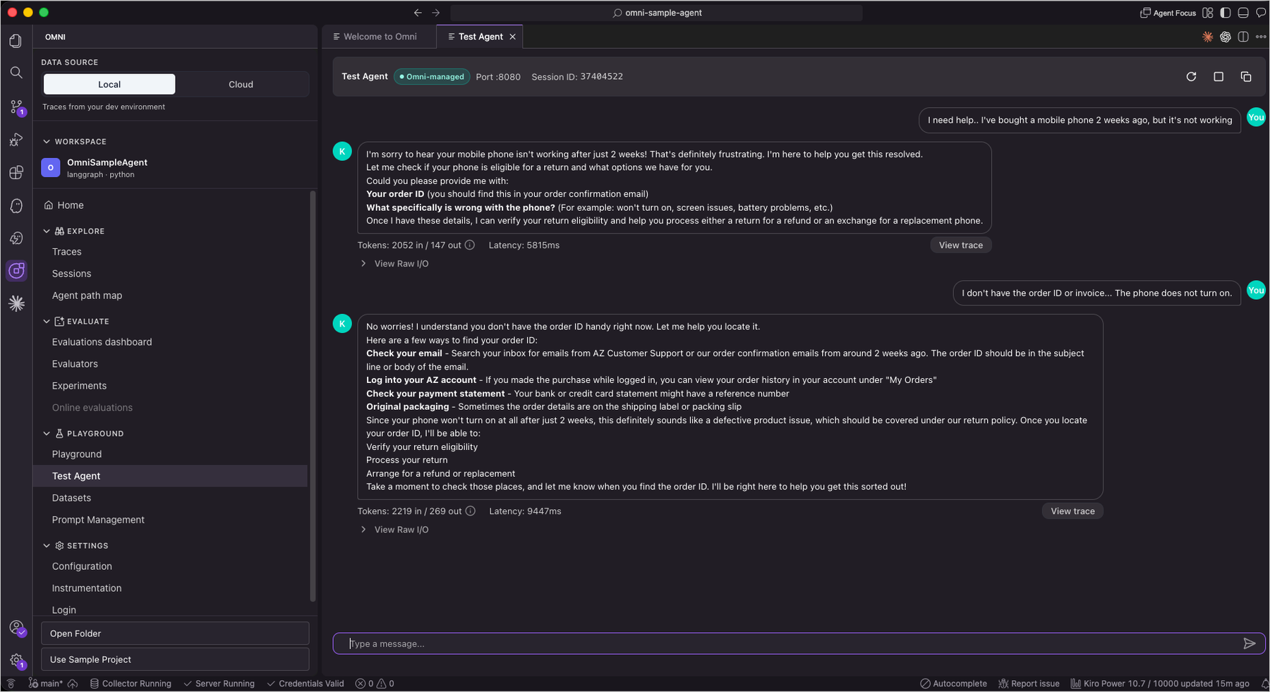
Runtime instances: persistent compute for production AI agents on Amazon Bedrock AgentCore

Post Syndicated from Sébastien Stormacq original https://aws.amazon.com/blogs/aws/runtime-instances-persistent-compute-for-production-ai-agents-on-amazon-bedrock-agentcore/

When you move AI agents from prototype to production, the infrastructure challenges multiply. Your agents need to persist state across multi-step workflows that run for hours or days. They need to coordinate with other agents, share context, and sometimes access GPUs for specialized tasks. Amazon Bedrock AgentCore runtime microVMs provide a fully managed environment for invocations that can run for up to 8 hours and support stateful workflows through managed session storage. Some workloads also benefit from dedicated, larger-capacity environments — for example, when agents need to run continuously for multiple days, access GPUs or the underlying OS, or run multiple collaborating agents on the same host.

Today, I’m happy to announce runtime instances, a new complementary compute option in Amazon Bedrock AgentCore Runtime that gives your agents persistent, managed infrastructure purpose-built for complex agent workloads.

What you get
Runtime instances provides AWS-managed EC2 infrastructure where you deploy multiple agents in a single runtime, each with their own dependencies and artifact types. Your agents can collaborate on the same host within shared sessions that persist for up to 14 days. The service supports GPU acceleration for compute-intensive tasks, session stop/restart to save costs during idle periods, and containerized deployments for teams that want to ship independently. For knowledge that needs to survive beyond a session, runtime instances pairs naturally with Amazon Elastic Block Store (Amazon EBS) and AgentCore Memory, which gives your agents long-term recall across sessions and environments.

Before today, if you wanted to keep your agents running for days or they needed GPU access, or multi-agent coordination, you had to build and manage that infrastructure yourself. You provisioned EC2 instances, configured networking, set up session management, handled scaling, and stitched together monitoring. Runtime instances handles all of that for you while integrating with the same AgentCore APIs, identity controls, and observability you already use with AgentCore Runtime microVMs.

A few things that should make agent developers smile: your agents can call each other as tools within a shared session, iterating autonomously until the job is done. You bring any framework (CrewAI, LangGraph, LlamaIndex, Strands) and any model. Packaging is minimal, a @app.entrypoint decorator and a zip file or container image. And if your workflow spans days, hibernate Monday night and resume Wednesday morning with everything intact.
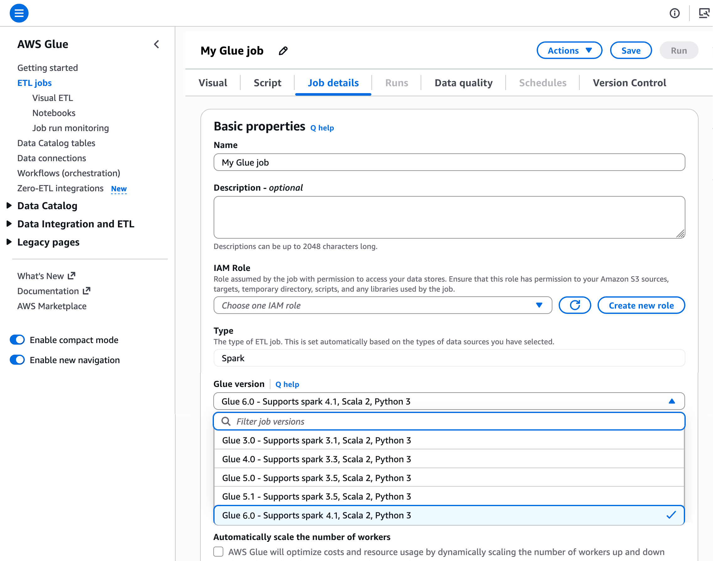
Runtime microVMs and runtime instances are complementary compute options that you can use independently or together through the same AgentCore runtime APIs. A lightweight orchestrator agent on runtime microVM can coordinate and dispatch work to specialized worker agents running on instances. The orchestrator handles API calls, task routing, and result aggregation using runtime microVM’s fast scaling, while workers on Instances perform compute-intensive tasks like code compilation, security scanning, or GUI automation that require persistent state and direct OS access.

Let me show you how it works
I built two agents for this demo: a code writer agent that generates Python code from natural language descriptions, and a code reviewer agent that analyzes the generated code for bugs, security issues, and style improvements. Both agents share the same file system, so the reviewer can read whatever the writer produces without any data transfer or API calls between them.

Here is the code writer (simplified, no error handling):

writer = Agent(
    model="us.anthropic.claude-sonnet-4-5-20250929-v1:0",
    system_prompt=(
        "You are a senior Python engineer. "
        "Given a task, return ONLY a single Python code block — no prose."
    ),
)

@app.entrypoint
def handler(event, context):
    task = event.get("task") or event.get("prompt")
    session_id = getattr(context, "session_id", None) or event.get("session_id")
    session_dir = SHARED_DIR / session_id
    session_dir.mkdir(parents=True, exist_ok=True)

    code = str(writer(task))
    (session_dir / "code.py").write_text(code)

    return {"agent": "writer", "wrote": str(session_dir / "code.py"), "code": code}

Here is the code reviewer agent (simplified, no error handling):

reviewer = Agent(
    model="us.anthropic.claude-sonnet-4-5-20250929-v1:0",
    system_prompt=(
        "You are a strict Python code reviewer. "
        "Given code, return 3 bullet points: bugs, style, suggestions."
    ),
)

@app.entrypoint
def handler(event, context):
    session_id = getattr(context, "session_id", None) or event.get("session_id")
    code_path = SHARED_DIR / session_id / "code.py"
    code = code_path.read_text()
    review = str(reviewer(f"Review this code:\n\n{code}"))

    return {"agent": "reviewer", "read": str(code_path), "review": review}

Each agent is a Python application using Strands Agents with an @app.entrypoint decorator and a model of its choice. I package each one as a zip file. For this demo, I use the AWS Management Console. You can also use the AgentCore CLI, the AWS Command Line Interface (AWS CLI) or infrastructure as code.

Step 1: Create a capacity provider.

A capacity provider defines the EC2 infrastructure your agents run on. In the AgentCore console, I select Runtime in the left navigation, then select the Capacity providers tab and Create capacity provider.

ACI Create Capcity Provider 1

I give it a Name, select Linux (64-bit ARM) as the Operating system, and choose c7g.2xlarge as the Allowed instance types. This gives me 8 vCPUs and 16 GiB of memory, enough for both agents to run comfortably side by side.

Further down, I configure the VPC, subnets, and security groups for network access. Under Storage configuration, I keep the default gp3 volume. Under Service access, I select Create a new service role and let the console create the infrastructure role that manages EC2 instances on my behalf.

I select Create capacity provider and wait a few seconds. The status moves to Active.

ACI Create Capacity Provider 2

ACI Create Capacity Provider 3

Note the capacity provider configuration summary: operating system, instance type, subnets, security group, instance profile, and infrastructure role. Once created, only the description can be edited, so verify your settings before you proceed.

ACI Create Capcity Provider 2

Step 2: Create a runtime and deploy the first agent.

Back on the Runtime page, I select Create runtime. I give it a Name, select Instances as the Compute type, and choose the Capacity provider I created in the previous step.

ACI Create Runtime 1

Under Agent source, I select S3 Source, then Upload to S3. I choose my agent zip file (ACIDemoWriter.zip), set the Language runtime to Python 3.13, and specify agent.py as the Agent entry point. This is the file that contains my @app.entrypoint decorated function. Under Permissions, I select Create default role to let the console provision the IAM role my agent needs.

ACI Create Runtime 2

I select Create runtime and wait for the status to become Ready.

I repeat the same process for my code reviewer agent. I create a second runtime, select the same capacity provider, upload my reviewer agent zip file, and wait for it to become Ready. Both agents now share the same underlying EC2 infrastructure.

AgentCore Runtime Instances - Agent ReadyThe console shows me a View invocation code section with ready-to-use Python, TypeScript, and JavaScript snippets to invoke my agent programmatically. But for this demo, I use the built-in test feature. I select Test on the writer agent’s page.

AgentCore Runtime Instances - Show invocation codeStep 3: Invoke agents and observe collaboration.

The Runtime playground opens. At the top, I see three fields: Runtime agent, Endpoint, and Session ID. The console generates a session ID automatically. I take note of it because I will reuse it with the reviewer agent.

In the Input field, I type a JSON payload asking the writer agent to generate code:

{"prompt": "write a fibonacci suite"}

I select Run. After a few seconds, the Output panel shows the agent’s response. The writer agent generated a Python module with two implementations of a Fibonacci sequence (a list-based function and a generator) and wrote it to /tmp/agentcore-session/ca5ec24d-07f5-4eeb-add1-5ba416bf9eb2/code.py. Notice the session ID in the file path. That directory is the shared file system for this session.

AgentCore Runtime Instances - Invoke code writer agent

Step 4: Invoke the reviewer agent in the same session.

Now I switch the Runtime agent dropdown to ACIDemoReviewer. The important part: I paste the same session ID (ca5ec24d-07f5-4eeb-add1-5ba416bf9eb2) in the Session ID field. This is what connects the two agents.

I type a simple prompt:

{"prompt": "review the code"}

I select Run. The reviewer agent reads the file the writer produced from the shared session directory and returns a detailed code review. It finds no critical bugs but suggests adding type hints, input validation, and simplifying the edge case handling.

AgentCore Runtime Instances - Invoke code reviewer agentThe two agents never exchanged messages or called each other’s APIs. They collaborated through the shared file system that runtime instances provide within a session. You can extend this pattern to any number of agents: a test agent that runs the code, a documentation agent that generates README files, a security agent that scans for vulnerabilities, all sharing the same working directory.

Key details
Here are a few things to know as you get started:

  • Supported OS: Linux (ARM64 and x86_64) at launch.
  • Session persistence: Sessions persist for up to 14 days.
  • Runtimes: Python 3.11-14 with native code support. Container images also supported.
  • GPU: Support for GPU-accelerated instance types.
  • Integration: Uses the same AgentCore APIs, identity, observability, and policy controls as AgentCore Runtime.
  • Pricing: Standard EC2 pricing plus a management fee for AgentCore orchestration.
  • Regions: US East (Ohio, N. Virginia), US West (Oregon), Asia Pacific (Mumbai, Singapore, Sydney, Tokyo), and Europe (Frankfurt, Ireland)

To get started, visit the runtime instance in Amazon Bedrock AgentCore documentation and create your first capacity provider.

— seb

Amazon DynamoDB now supports real-time vector search at any scale

Post Syndicated from Esra Kayabali original https://aws.amazon.com/blogs/aws/amazon-dynamodb-now-supports-real-time-vector-search-at-any-scale/

Today, we’re announcing the general availability of vector search in Amazon DynamoDB. You can now store vector embeddings alongside your operational data in DynamoDB and run similarity searches directly against that data, without replicating it to a separate vector store.

DynamoDB supports native vector search with single-digit millisecond latency at 99%+ recall, and is designed for any scale, even trillions of vectors. There are no servers to provision, patch, or manage, and no software to install, maintain, or operate. The service has no versions, no maintenance windows, and zero downtime maintenance.

Vector indexes have no storage limits and scale horizontally as your data grows. You can now build applications that require semantic retrieval on agentic memory, retrieval augmented generation, recommendation engines, personalized experiences, anomaly detection, and more using DynamoDB and its native vector search.

If your application already uses DynamoDB, adding vector search previously required copying data into a dedicated vector database while maintaining a synchronization pipeline between the two services. This added operational overhead, data movement costs, licensing costs, and the challenge of maintaining predictable low latency at scale. With vector search built into DynamoDB, your vectors and operational data share the same serverless infrastructure and the same pay-per-request pricing model.

Vector search in DynamoDB introduces a new index type that you create on an attribute storing vector embeddings. You generate embeddings using a model of your choice, such as Amazon Bedrock Titan Text Embeddings, Cohere Embed, or OpenAI text embedding models, and store them as a list of floats in your table using a standard PutItem call. You then create a vector index on that attribute and specify the number of dimensions, the distance function, and any non-vector attributes you want to use as filters to narrow search results at query time. The SearchVectors API accepts a query vector, the number of results to return (up to 100), and optional filter conditions. It returns results ranked by similarity.

Use vector search in DynamoDB when your operational data already lives in DynamoDB and you want to add similarity search without provisioning a separate database or managing a synchronization pipeline. DynamoDB is fully serverless, so vector search scales automatically with no infrastructure to manage. It supports up to 4096 dimensions, Euclidean, Cosine, and Dot product distance functions, and inline filtering.

Getting started with vector search in DynamoDB
This walkthrough shows how to add vector search to an existing DynamoDB table using the DynamoDB console. The scenario contains an online sporting goods store with a product catalog table. Each item has standard operational attributes such as productId, category, description, marketplace, name, and price. The goal is to add semantic search so shoppers can find products using natural language queries rather than exact keyword matches.

1. Prepare DynamoDB table
To enable semantic search, I first generate vector embeddings for the product descriptions already in my table. Embeddings are numerical representations of text generated by a machine learning model that capture the meaning of the content. Two items with similar descriptions will have embeddings that are close to each other in vector space, which is what makes similarity search possible.

I can generate embeddings using Amazon Bedrock Titan Text Embeddings or another embedding model, then add them to my table using the AWS Management Console, AWS Command Line Interface (AWS CLI), AWS SDKs, AWS CloudFormation, or other infrastructure-as-code (IaC) tools.

For an existing table like ProductCatalog, I add the embeddings to each item as a new attribute named descriptionEmbedding using an UpdateItem call. DynamoDB stores vector embeddings using its existing List data type. Each element in the list is a Number that represents a single float value of the embedding vector. This means I do not need a new data type or schema change to start storing vectors alongside my existing operational attributes.

2. Create vector index
In the DynamoDB console, open the ProductCatalog table and choose the Indexes tab. I choose Create vector index. On the Create vector index page, I fill in the index details as follows. I enter ProductDescriptionIndex as the Index name and descriptionEmbedding as the Vector attribute.

I enter the number of Dimensions that matches my embedding model’s output and select Cosine as the Distance function. Cosine measures the angle between vectors rather than their magnitude, which makes it effective for comparing semantic similarity of text embeddings. Vector search in DynamoDB also supports Euclidean and Dot product distance functions.

  • Euclidean: Use when the magnitude of the vectors is meaningful, such as clustering items by a numeric value like purchase count.
  • Dot product: Use when both direction and magnitude matter, such as in recommendation systems that weight interest alignment and frequency together. As a general rule, match the distance function to the one used to train your embedding model for the best accuracy.

I enter marketplace as the Partition key. The vector index partition key controls how DynamoDB distributes vectors across partitions, allowing the index to scale out while maintaining predictable latencies. Each search is scoped to a single partition key value, so a product catalog serving multiple marketplaces can search within one marketplace’s inventory without scanning the entire index. The partition key is optional, but recommended for large datasets with high query throughput.

I expand Inline filter attributes and add category as a filter attribute. This helps me narrow search results to a specific product category at query time. Filter conditions support exact-match values only; range conditions such as BETWEEN or BEGINS_WITH are not supported. I leave Attribute projections set to All so that all table attributes are returned with my search results. Choose Create vector index and wait for the index status to change to Active.

3. Run vector search
I generate a query vector from a natural language search term such as “lightweight running shoes for summer” using the same embedding model I used for the product descriptions. In the DynamoDB console, I choose Explore items in the left navigation pane and select the ProductCatalog table.

Choose Search to switch to vector search mode. I select ProductDescriptionIndex from the Select a vector index dropdown, paste the query vector into the Search vector field, and set Number of results (Top K) to 5. I enter US as the Partition key value to scope the search to the US marketplace. I expand Inline filter attributes and set category equal to footwear to narrow the search to footwear products only. Now, choose Run.

DynamoDB returns the five most semantically similar products in the footwear category, ranked by similarity score, alongside the standard operational attributes such as name and price in the same response. The similarity score’s meaning depends on the distance function selected for the index. For Cosine and Euclidean distance functions, lower similarity score values indicate higher similarity, with a score of 0 indicating identical vectors. For the dot product distance function, higher similarity score values indicate higher similarity.

To interact with vector search programmatically, including calling APIs and searching documentation, try the AWS MCP Server and plugins with your preferred AI coding tool. To learn more, visit the Amazon DynamoDB Developer Guide.

Get started today
Vector search in Amazon DynamoDB is generally available in all commercial AWS Regions, including the AWS GovCloud (US) Regions. For Regional availability and a future roadmap, visit the AWS Capabilities by Region. For pricing details, visit the Amazon DynamoDB pricing page.

Start exploring vector search in DynamoDB today and send feedback to AWS re:Post for Amazon DynamoDB or through your usual AWS Support contacts.

— Esra

Analyze and remediate technical debt autonomously with AWS Transform – continuous modernization

Post Syndicated from Ritik Khatwani original https://aws.amazon.com/blogs/devops/analyze-and-remediate-technical-debt-autonomously-with-aws-transform-continuous-modernization/

Introduction

In a recent post, my colleague Micah Walter introduced AWS Transform – continuous modernization in public preview. Today, this capability is generally available in regions supported for AWS Transform .

Development velocity continues to increase. But velocity without maintenance accumulates technical debt at speed. The faster software scales, the faster technical debt compounds. At the same time, more sophisticated exploits and attack vectors are emerging – and the risk is increasing (Figure 1). For organizations, this makes staying on top of tech debt and maintaining a strong security posture across an increasing sphere of responsibility not only important, but business-critical.

Two pie-circle diagrams connected by an arrow labeled "AGENTIC AI." In the left circle, most of the area is labeled "BUY, SAAS, COTS" while a small blue wedge labeled "BUILD, MAINTAIN" faces three arrows labeled "VULNERABILITIES." In the right circle, the blue "BUILD, MAINTAIN" section has grown to roughly half the circle and faces many more vulnerability arrows, illustrating how agentic AI expands the amount of code organizations build and maintain — and the corresponding vulnerability surface.

Figure 1: Changing landscape of software maintenance

To contend with compounding technical debt, engineering organizations have typically stitched together point tools, spent app-by-app cycles wasting engineering capacity, and relied on self-reports for status that lags reality and hides regressions.

This is the problem continuous modernization capability was built to solve: shift code transformation from a periodic project into an automated, always-on practice. Rather than scheduling modernization sprints or relying on manual audits, your repositories are analyzed on demand or on a recurring schedule, with findings prioritized by severity and impact, and validated pull requests are generated autonomously to resolve them.

In this post, I’ll recap the preview launch and then I’ll walk you through additional capabilities we’ve added since. I’ll also show how you can use it today to get started.

What continuous modernization provides

AWS Transform – continuous modernization connects to your source control systems (GitHub, GitLab, Bitbucket, or local repositories), scans repositories, and generates prioritized findings. At your direction, it autonomously creates pull requests with validated code changes.

The capability supports several analysis types:

  • Rapid tech debt analysis: fast metadata-only scans of package manifests (pom.xml, package.json, requirements.txt) to identify stale versions and outdated dependencies
  • Comprehensive tech debt analysis: deep code-level analysis examining source code for debt patterns, code quality issues, architecture concerns, and improvement opportunities
  • Security analysis: Common vulnerability detection within the source code and dependencies via AWS Security Agent (now part of AWS Continuum)
  • Agentic readiness: assesses your code base readiness for agent integration
  • Modernization readiness: evaluates candidates for containerization, serverless migration, and platform upgrades
  • Custom analysis: run your own transformation definition as an analysis, including organization-specific policies your platform team already enforces

You can run these analyses on demand or schedule them on a recurring cadence. The system accumulates findings over time, giving you trend data and portfolio-wide visibility that periodic manual audits can’t match.

Initiate and schedule recurring analysis from the AWS Transform web app

We’re excited to add the ability to connect your source code management (SCM) provider and initiate an analysis directly from the AWS Transform web application so you can get value from real insights faster than before (Figure 2). You can also schedule recurring analysis, review findings, and create remediations from within the web app. To learn more about the web app and how to set it up, see AWS Transform web application.

Screen recording of the AWS Transform Continuous Modernization console (N. Virginia region). A "Connect new source" dialog is filled in with GitHub as the provider, then repositories refresh and "agentcore-samples" is selected from the awslabs-agentcoresamples source. A new analysis is configured with type "Tech debt (comprehensive)" and named "agentcore samples tech debt comprehensive." In the Schedule step, "Recurring" is chosen with a weekly cadence on Mondays, a start date of 2026/07/28, and a start time, ending with the "Run now and schedule" button.

Figure 2: Set up continuous modernization in the AWS Transform web application

Interact via your IDE or terminal with the new CLI and developer tools

The new version of the AWS Transform CLI and it’s atx ct(v3.8.0) introduce additional capabilities that simplify how you setup and work with continuous modernization. The new atx ct remote sub-commands allow you to provision infrastructure and run scheduled analyses and remediations with Amazon Elastic Compute Cloud (Amazon EC2) and AWS Batch (Figure 3). To learn more about the CLI commands, refer to working with continuous modernization. The updated AWS Transform Kiro power and plugin make it even easier to configure your source repositories and run analyses directly from your IDE or terminal. To learn more, see developer tools.

You can also leverage labels with your repositories to group them and organize operations in batches. In the example below, I create a subset of repositories from my GitHub organization that I want to run agentic readiness analysis on and trigger a one-time analysis.

Screen recording of a macOS zsh terminal running AWS Transform CLI commands. First, atx ct repository update tags two repositories (ritikk::ecsdemo-nodejs and ritikk::ecsdemo-frontend) with the label "ecs-demos"; the output confirms "Bulk label update complete: Targeted 2, Updated 2." Then atx ct remote analysis --types "agentic-readiness" --mode "batch" --labels "ecs-demos" --sources "ritikk" --stack-name "AtxInfrastructureStack" kicks off a batch analysis. Pre-flight checks pass, a Lambda function is invoked, an S3 manifest is written, and two jobs are submitted to Batch with a batch ID and a poll command shown to check status.

Figure 3: Use the AWS Transform cli to analyze your repositories

Real-world results

Across industries, partners and enterprises are already seeing the impact of continuous modernization. The results speak to a consistent theme: what used to take months of manual effort now happens in minutes, at a scale that was previously impractical with manual review.

From weeks of manual assessment to insights in days

Quantiphi ran continuous modernization across a large portfolio and compressed a multi-week assessment into a matter of days:

“At Quantiphi, we’re helping enterprises accelerate application modernization through AI-powered engineering. Using AWS Transform continuous modernization, we analyzed more than 500 repositories and uncovered over 3,000 technical debt findings in less than a week, a time frame that traditionally required nearly three weeks of manual assessment. By automating technical debt discovery and providing actionable remediation insights, we reduced assessment effort by more than 60%, accelerated modernization planning, and enabled our customers to focus engineering investments on innovation instead of analysis. We believe AWS Transform continuous modernization is a foundational capability for delivering continuous, AI-driven enterprise modernization at scale.”

Sanchit Jain, Migration and Modernization Practice Leader, Quantiphi AWS Practice

Shifting from reactive maintenance to proactive modernization

For Hexaware, the value is in continuously surfacing what needs attention across large portfolios, so teams can get ahead of debt rather than react to it:

“At Hexaware, we’re constantly looking for ways to help clients modernize faster while controlling cost and complexity. AWS Transform continuous modernization provides a scalable approach to identifying technical debt, modernization opportunities, and AI-readiness gaps across large application portfolios. By automating analysis and continuously surfacing remediation recommendations, organizations can shift from reactive maintenance to proactive modernization. This capability has the potential to significantly accelerate transformation roadmaps and help enterprises build more resilient, future-ready applications, very quickly.”

Inderjeet Gurtatta, Vice President, Hexaware Technologies

An 80 percent reduction in assessment time

Tech Mahindra measured the impact directly, cutting assessment time from 40 hours to 8 across 25 repositories:

“Achieving an 80 percent reduction in assessment time, from 40 hours down to 8, across 25 enterprise repositories is just the beginning of what we see as a transformative shift in how organizations approach continuous modernization. AWS Transform’s scanning and analysis engine is solid, and the structured output allows our teams to validate findings quickly and build prioritized remediation plans with confidence. As the platform matures with features like scan resume capabilities and broader platform support, we expect to embed AWS Transform continuous modernization into our standard delivery methodology while maintaining the depth and accuracy our enterprise clients demand.”

Sanjeev Agarwal, Global Head of AWS Business, Tech Mahindra

Uncovering risks that traditional scanners miss

Cybage found that the continuous modernization capability surfaced hidden security risks that conventional scans overlooked, then fed those findings into their own delivery framework:

“AWS Transform continuous modernization completes codebase analysis in under an hour, work which normally takes weeks, while uncovering risks that traditional scanners miss like disabled security warnings, vulnerable code copied into applications, and security controls intentionally switched off. Cybage’s CLEAR Framework builds on these findings by converting them into a prioritized, customer-specific modernization plan with confidence scoring, technical-debt measurement, and integration with tools like GitHub, Jira, and SonarQube. Together, AWS Transform discovers hidden risks at speed, and CLEAR determines what matters most and how teams move from analysis to execution.”

Mohammad Mahdee-uz Zaman, Vice President, AWS Strategic Alliances, Cybage Software Inc.

Straight from discovery to a concrete migration plan

3Pillar moved directly from discovery to an actionable migration plan:

“For most IT leaders, application modernization is the bane of their existence. We put AWS Transform continuous modernization to the test across more than 25 repos, and came away very impressed. Analysis that would have taken our engineers an estimated 3-4 weeks of manual code reviews surfaced in an hour, uncovering over 190 tech debt findings, including outdated dependencies, dead code, and migration risks. The service’s ability to build migration rules purpose-built for each repo let us move straight from discovery to a concrete migration plan, without weeks of manual mapping. Based on our testing, we estimate AWS Transform continuous modernization can cut 40-50% off the overall modernization lifecycle. This speed means tech leaders can embark on modernization initiatives with confidence that it won’t drag on for many years.”

Pankaj Chawla, CTO, 3Pillar

Conclusion

AWS Transform – continuous modernization helps you go from one-off projects and campaigns to a fully operational tech debt management program: connecting sources, running analyses, triaging findings, launching remediation campaigns, and scheduling recurring scans. The web app dashboard and reports provide prioritization signals directly from your code. When a repository diverges from your baseline, the next analysis can surface the change and help teams understand its severity and breadth. This reduces reliance on manual status collection and periodic code-health audits.

To get started, you can access the capability through the AWS Transform Kiro power, the AWS Transform web application, or directly via the atx ct CLI. To learn more, visit the AWS Transform documentation.

Ritik Khatwani

Ritik Khatwani

Ritik is a Sr Worldwide Specialist Solutions Architect at AWS based in New York City. He has deep expertise in software engineering and currently works with customers to modernize their development workflows using generative AI.

Introducing Amazon Simple Email Service (SES) pricing plans

Post Syndicated from Advait Gomkale original https://aws.amazon.com/blogs/messaging-and-targeting/introducing-amazon-simple-email-service-ses-pricing-plans/

Businesses rely on email to deliver critical notifications, nurture customer relationships, and grow revenue. But their success depends on more than just sending the right message. It depends on emails getting delivered to the inbox and ultimately getting read. When emails land in spam or go unread, the business impact is real and measurable: missed engagement, eroded customer trust, and lost revenue.

Most email providers offer capabilities to help improve deliverability, including dedicated sending infrastructure, reputation monitoring, address validation, and inbox placement testing. But these capabilities are typically sold as individual add-ons, each priced separately. Reaching the inbox consistently shouldn’t require evaluating dozens of options independently.

That changes today with Amazon SES pricing plans. Pick a plan, and the right capabilities are already included at up to 22% less than purchasing them individually.

Amazon SES pricing plans

Amazon SES offers three plans: Essentials, Pro, and Enterprise. Each builds on the one before it, offering more capability, so you choose the one that fits your email needs.

Essentials

Get started with Amazon SES. Monitor how emails perform and get insights to help improve deliverability over time.

Send email reliably at scale and see what’s happening: which emails are landing, which are bouncing, and what needs attention. Essentials gives you the data and recommendations to guide your improvements, with the flexibility to upgrade to Pro as your deliverability needs grow.

Pro

Get higher deliverability with dedicated infrastructure and proactive reputation protection. Reach the inbox consistently as sending scales.

Pro shifts deliverability from reactive to proactive. With Pro, your sending runs on dedicated IPs, keeping your reputation isolated from other senders. Invalid addresses are caught before they bounce, and you see inbox placement across providers your domains send through, not just within SES. Pro helps you prevent problems, not just discover them after the fact.

Enterprise

Get the most out of Amazon SES. Reach the inbox reliably, stay resilient globally, and isolate sending reputation across workloads.

Everything in Pro, plus resilience that keeps email flowing if a region goes down, reputation isolation across separate workloads, and an annual deliverability assessment. This is the most comprehensive SES experience available.

For full pricing details and a complete feature comparison across all three plans, visit the Amazon SES Pricing page.

Getting started

Starting July 21, 2026, all new SES accounts begin on the Essentials plan. Returning customers who have not sent or processed email through SES since June 1, 2025 also begin on the Essentials plan. From there, you can upgrade to Pro or Enterprise, or switch to à-la-carte pricing at any time. Customers who have sent or processed email through SES on or after June 1, 2025 remain on à-la-carte pricing and can switch to a plan anytime.

If you are new to AWS, the AWS Free Tier provides up to $200 in credits during your first six months that you can apply toward Amazon SES pricing plans. As of July 21, 2026, the SES-specific free tier (3,000 email message charges per month for your first 12 months after first SES use) is no longer available for new customers. If you are currently on the SES-specific free tier, your benefits continue for the remainder of your 12-month period.

To get started, sign in to the Amazon SES console and navigate to the Pricing plan section. To learn more, visit the Amazon SES Pricing page or explore the Amazon SES documentation.


About the Authors

Amazon SQS turns 20: Two decades of reliable messaging at scale

Post Syndicated from Esra Kayabali original https://aws.amazon.com/blogs/aws/amazon-sqs-turns-20-two-decades-of-reliable-messaging-at-scale/

On July 13, 2006, we launched Amazon Simple Queue Service (Amazon SQS) as one of the first three services available to customers, alongside Amazon EC2 and Amazon S3. We had learned firsthand that distributed systems need a reliable way to pass messages between components without creating tight dependencies. If one service called another directly and that service was slow or unavailable, failures cascaded through the entire system. Message queuing solved this by letting services communicate asynchronously: a producer could drop a message into a queue and move on, while a consumer picked it up when ready. This approach kept individual service failures from affecting the rest of the system.

When Amazon SQS launched publicly in July 2006, it made this pattern available to every AWS customer. Twenty years later, that core function, decoupling producers from consumers, remains the reason customers use SQS. The scale, performance, and operational controls around it look very different now though.

Jeff Barr covered the first 15 years of SQS milestones in his 15th anniversary post, from the original 8 KB message limit in 2006 through FIFO queues, server-side encryption, and Lambda integration. Over the last five years, we have continued to scale SQS, added stronger security defaults, and introduced new capabilities that address increasingly complex workload patterns.

Key milestones between 2021 and 2026
High throughput mode for FIFO queues (2021): In May 2021, we launched general availability of high throughput mode for FIFO queues, supporting up to 3,000 transactions per second (TPS) per API action, a tenfold increase over the previous limit. We continued raising this ceiling over the following two years: to 6,000 TPS in October 2022, to 9,000 TPS in August 2023, and to 18,000 TPS in October 2023, before reaching 70,000 TPS per API action in select Regions by November 2023.

Server-side encryption with SSE-SQS (2021): In November 2021, we introduced server-side encryption with Amazon SQS-managed encryption keys (SSE-SQS), giving customers an encryption option that required no key management. In October 2022, we made SSE-SQS the default for all newly created queues, so customers no longer needed to explicitly enable it.

Dead-letter queue redrive enhancements (2021): We progressively expanded how customers recover unconsumed messages from dead-letter queues. In December 2021, we added DLQ redrive to source queue directly in the SQS console. In June 2023, we extended this capability to the AWS SDK and CLI through new APIs, including StartMessageMoveTask, CancelMessageMoveTask, and ListMessageMoveTasks. In November 2023, we added redrive support for FIFO queues.

Attribute-based access control, ABAC (2022): In November 2022, we introduced ABAC, giving customers the ability to configure access permissions based on queue tags rather than maintaining static policies as resources scaled.

JSON protocol support (2023): In November 2023, we added support for the JSON protocol in the AWS SDK, reducing end-to-end message processing latency by up to 23% for a 5 KB payload and lowering client-side CPU and memory usage.

Amazon EventBridge Pipes console integration (2023): We added the ability to connect a queue directly to EventBridge Pipes from the SQS console, routing messages to a broad range of AWS service targets without writing custom integration code.

Extended Client Library for Python (2024): We brought the Extended Client Library, previously available for Java, to Python developers, allowing messages up to 2 GB to be sent through SQS by storing the payload in Amazon S3 and passing a reference through the queue.

FIFO in-flight message limit increase (2024): We increased the in-flight message limit for FIFO queues from 20,000 to 120,000 messages, so consumers can process significantly more messages concurrently without being constrained by the previous ceiling.

Fair queues for multi-tenant workloads (2025): We introduced fair queues to mitigate the noisy neighbor problem in multi-tenant standard queues. By including a message group ID when sending messages, customers can prevent a single tenant from delaying message delivery for others, without any changes required on the consumer side.

1 MiB maximum message payload size (2025): We increased the maximum message payload from 256 KiB to 1 MiB for both standard and FIFO queues, helping customers send larger messages without offloading data to external storage. AWS Lambda event source mapping for SQS was updated in parallel to support the new payload size.

The constant underneath the change
Despite two decades of feature additions, the fundamental use case for SQS has not shifted. Customers use it to decouple services, buffer bursts of traffic, and build systems that stay resilient when individual components fail. That same pattern now extends to AI workloads. Customers use SQS queues to buffer requests to large language models, manage inference throughput, and coordinate communication between autonomous AI agents operating as independent services. For an example of this architecture in practice, read Creating asynchronous AI agents with Amazon Bedrock.

To learn more about Amazon SQS, visit the Amazon SQS product page, review the developer guide, or explore recent updates on the AWS Blogs.

— Esra