Ransomware has evolved from simple digital extortion into a structured, profit-driven criminal enterprise. Over time, it has led to the development of a complex ecosystem where stolen data is not only leveraged for ransom, but also sold to the highest bidder. This trend first gained traction in 2020 when the Pinchy Spider group, better known as REvil, pioneered the practice of hosting data auctions on the dark web, opening a new chapter in the commercialization of cybercrime.
In 2025, contemporary groups such as WarLock and Rhysida have embraced similar tactics, further normalizing data auctions as part of their extortion strategies. By opening additional profit streams and attracting more participants, these actors are amplifying both the frequency and impact of ransomware operations. The rise of data auctions reflects a maturing underground economy, one that mirrors legitimate market behavior, yet drives the continued expansion and professionalization of global ransomware activity.
Anatomy of victim data auctions
Most modern ransomware groups employ double extortion tactics, exfiltrating data from a victim’s network before deploying encryption. Afterward, they publicly claim responsibility for the attack and threaten to release the stolen data unless their ransom demand is met. This dual-pressure technique significantly increases the likelihood of payment.
In recent years, data-only extortion campaigns, in which actors forgo encryption altogether, have risen sharply. In fact, such incidents doubled in 2025, highlighting how the threat of data exposure alone has become an effective extortion lever. Most ransomware operations, however, continue to use encryption as part of their attack chain.
Certain ransomware groups have advanced this strategy by introducing data auctions when ransom negotiations with victims fail. In these cases, threat actors invite potential buyers, such as competitors or other interested parties, to bid on the stolen data, often claiming it will be sold exclusively to a single purchaser. In some instances, groups have been observed selling partial datasets, likely adjusted to a buyer’s specific budget or area of interest, while any unsold data is typically published on dark web leak sites.
This process is illustrated in Figure 1, under the assumption that the threat actor adheres to their stated claims. However, in practice, there is no guarantee that the stolen data will remain undisclosed, even if the ransom is paid. This highlights the inherent unreliability of negotiating with cybercriminals.
⠀
Figure 1 – Victim data auctioning process
⠀
This auction model provides an additional revenue stream, enabling ransomware groups to profit from exfiltrated data even when victims refuse to pay. It should be noted, however, that such auctions are often reserved for high-profile incidents. In these cases, the threat actors exploit the publicity surrounding attacks on prominent organizations to draw attention, attract potential buyers, and justify higher starting bids.
This trend is likely driven by the fragmentation of the ransomware ecosystem following the recent disruption of prominent threat actors, including 8Base and BlackSuit. This shift in cybercrime dynamics is compelling smaller, more agile groups to aggressively compete for visibility and profit through auctions and private sales to maintain financial viability. The emergence of the Crimson Collective in October 2025 exemplified this dynamic when the group auctioned stolen datasets to the highest bidder. Although short-lived, this incident served as a proof of concept (PoC) for the growing viability of monetizing data exfiltration independently of traditional ransom schemes.
Threat actor spotlight
WarLock
The WarLock ransomware group has been active since at least June 2025. The group targets organizations across North America, Europe, Asia, and Africa, spanning sectors from technology to critical infrastructure. Since its emergence, WarLock has rapidly gained prominence for its repeated exploitation of vulnerable Microsoft SharePoint servers, leveraging newly disclosed vulnerabilities to gain initial access to targeted systems.
The group adopts double extortion tactics, exfiltrating data from the victim’s systems before deploying its ransomware variant. From a recent incident Rapid7 responded to, we observed the threat actor exfiltrating the data from a victim to an S3 bucket using the tool Rclone. An anonymized version of the command used by the threat actor can be found below:
WarLock operates a dedicated leak site (DLS) on the dark web, where it lists its victims. From the outset of its operations, the group has auctioned stolen data, publishing only the unsold information online (Figure 2). The group further mentions that the exfiltrated data may be sold to third parties if the victim refuses to pay in their ransom note (Figure 3).
⠀
Figure 2 – Example of purchased data
⠀
Figure 3 – WarLock ransom note
⠀
Although WarLock shares updates on the progress and results of these auctions through its DLS, it also relies heavily on its presence on the RAMP4 cybercrime forum to attract potential buyers (Figure 4). This approach likely allows WarLock to reach a wider buyer base by publishing these posts under the relevant thread “Auction \ 拍卖会”. It should be noted that WarLock is assessed to be of Chinese origin, which is further supported by the Chinese-language reference in this thread title.
⠀
Figure 4 – Mention of an auction on WarLock’s DLS
⠀
Using the alias “cnkjasdfgd,” the group advertises details about the nature and volume of exfiltrated data, along with sample files (Figure 5). WarLock further directs interested buyers to its Tox account, a peer-to-peer encrypted messaging and video-calling platform, where the auctions appear to take place.
⠀
Figure 5 – WarLock’s post on RAMP4
⠀
This approach appears to be highly effective for WarLock. Despite being a recent entrant to the ransomware ecosystem, the group has reportedly sold victim data in approximately 55% of its claimed attacks, accounting for 55 victims to date as of November 2025, demonstrating significant traction within underground markets. The remaining victims’ data has been publicly released on the group’s DLS, following unsuccessful ransom negotiations and a lack of interested buyers.
Rhysida
The Rhysida ransomware group was first identified by cybersecurity researchers in May 2023. The group primarily targets Windows operating systems across both public and private organizations in sectors such as government, defense, education, and manufacturing. Its operations have been observed in several countries, including the United Kingdom, Switzerland, Australia, and Chile. The threat actors portray themselves as a so-called “cybersecurity team” that assists organizations in securing their networks by exposing system vulnerabilities.
Rhysida maintains an active DLS, where it publishes data belonging to victims who refuse to pay the ransom, in alignment with double extortion tactics. Since at least June 2023, the group has also conducted data auctions via a dedicated “Auctions Online” section of its DLS. These auctions typically run for seven days, and Rhysida claims that each dataset is sold exclusively to a single buyer. As of mid-October 2025, the group was hosting five ongoing auctions, with starting prices ranging from 5 to 10 Bitcoin (Figure 6).
⠀
Figure 6 – Example of an auction on Rhysida’s DLS
⠀
Once the auction period ends, Rhysida publicly releases any unsold data on its DLS (Figure 7). Instead, if the auction is successful, the data is marked as “sold”, without being released on the group’s DLS (Figure 8). In many cases, the group publishes only a subset of the stolen data, often accompanied by the note “not sold data was published” (Figure 9).
⠀
Figure 7 – Example of full data release on Rhysida’s DLS
⠀
Figure 8 – Example of sold data on Rhysida’s DLS
⠀
Figure 9 – Example of partial data release on Rhysida’s DLS
⠀
With 224 claimed attacks to date as of November 2025, approximately 67% resulting in full or partial data sales, auctions represent a significant additional revenue stream for Rhysida. The group’s auction model appears to be considerably more effective than WarLock’s (Figure 10), likely due to Rhysida’s established reputation within the cybercrime ecosystem and its involvement in several high-profile attacks.
⠀
Figure 10 – Overview of auction outcomes
Conclusion
The cyber extortion ecosystem is undergoing a profound transformation, shifting from traditional ransom payments to a diversified, market-driven model centered on data auctions and direct sales. This evolution marks a turning point in how ransomware groups generate revenue, transforming what were once isolated extortion incidents into structured commercial transactions.
Groups such as WarLock and Rhysida exemplify this shift, illustrating how ransomware operations increasingly mirror illicit e-commerce ecosystems. By auctioning exfiltrated data, these actors not only create additional revenue streams but also reduce their dependence on ransom compliance, monetizing stolen data even when victims refuse to pay. This approach has proven particularly lucrative for these threat actors, likely setting a precedent for newer extortion groups eager to replicate their success.
As a result, proprietary and sensitive data, including personally identifiable and financial information, is flooding dark web marketplaces at an unprecedented pace. This expanding secondary market intensifies both the operational and reputational risks faced by affected organizations, extending the impact of an attack well beyond its initial compromise.
To adapt to this evolving threat landscape, organizations must move beyond reactive crisis management and embrace a proactive, intelligence-driven defense strategy. Continuous dark web monitoring, early breach detection, and the integration of cyber threat intelligence into response workflows are now essential. In a world where stolen data functions as a tradable commodity, resilience depends not on negotiation but on vigilance, preparedness, and rapid action.
Twonky Server version 8.5.2 is susceptible to two vulnerabilities that facilitate administrator authentication bypass on Linux and Windows. An unauthenticated attacker can improperly access a privileged web API endpoint to leak application logs, which contain encrypted administrator credentials (CVE-2025-13315). As a result of the use of hardcoded encryption keys, the attacker can then decrypt these credentials and login as an administrator to Twonky Server (CVE-2025-13316). Exploitation results in the unauthenticated attacker gaining plain text administrator credentials, full administrator access to the Twonky Server instance, and control of all stored media files. These vulnerabilities are tracked as CVE-2025-13315 and CVE-2025-13316.
These vulnerabilities have not been patched. Despite making contact with the vendor, and the vendor confirming receipt of our technical disclosure document, the vendor ceased communications after disclosure. They stated that a patch wouldn’t be possible, even with a disclosure timeline extension, and subsequent follow-up attempts on our part were unsuccessful. As such, the vulnerable version 8.5.2 is the latest available.
Product description
Twonky Server is media server software marketed to both organizations and individuals. It’s generally designed to run on embedded systems, such as NAS devices and routers, for media organization, access, and streaming. At the time of publication, Shodan returns approximately 850 Twonky Server services exposed to the public internet.
Credit
These issues were discovered and reported to Lynx Technology by Ryan Emmons, Staff Security Researcher at Rapid7. The vulnerabilities are being disclosed in accordance with Rapid7’s vulnerability disclosure policy. This work is based on the previous Twonky Server research published by Sven Krewitt.
Vulnerability details
CVE
Description
CVSS
CVE-2025-13315
An unauthenticated remote attacker can bypass web service API authentication controls to leak a log file and read the administrator’s username and encrypted password.
The application uses hardcoded encryption keys across installations. An attacker with an encrypted administrator password value can decrypt it into plain text using these hardcoded keys.
The testing target was Twonky Server 8.5.2, the latest version available at the time of research. Rapid7 identified two security vulnerabilities as part of this research project, which are outlined in the table above. These vulnerabilities were tested against Twonky Server installed on two different operating systems: Ubuntu Linux 22.04.1 and Windows Server 2022. When exploited, these vulnerabilities effectively serve as a patch bypass for the security mitigations introduced in response to the two vulnerabilities disclosed by Risk Based Security in 2021.
CVE-2025-13315
In 2021, the security firm Risk Based Security disclosed an improper API access vulnerability in Twonky Server, for which no CVE is assigned. Their approach was to leak the administrator’s username and obfuscated password via requests to /rpc/get_option?accessuser and /rpc/get_option?accesspwd, which previously did not enforce authentication checks. In the patch, authentication checks were implemented for the /rpc web API. However, some administrator RPC API endpoints, such as log_getfile, are still accessible without authentication via alternative routing.
00461ddf                                if (!check_path(&arg1[2], "/rpc/info_status"))
00461ddf                                {
00461fc8                                    if (check_path(&arg1[2], "/rpc/stop"))
00461fcf                                        goto label_461de5;
00461fcf
00461fe4                                    if (check_path(&arg1[2], "/rpc/stream_active"))
00461fe4                                        goto label_461de5;
00461fe4
00461ff9                                    if (check_path(&arg1[2], "/rpc/byebye"))
00461ff9                                        goto label_461de5;
00461ff9
0046200e                                    if (check_path(&arg1[2], "/rpc/wakeup"))
0046200e                                        goto label_461de5;
0046200e
00462023                                    if (check_path(&arg1[2], "/rpc/get_option?language"))
00462023                                        goto label_461de5;
00462023
00462043                                    if (check_path(&arg1[2], "/rpc/get_option?multiusersupportenabled")
00462043                                            || !(var_480_1 & 1))
[..SNIP..]
004621af                                            *(uint64_t*)((char*)arg1 + 0x828) = "text/plain; charset=utf-8";
004621af
004621c9                                            if (check_path(&arg1[2], "/rpc/log_getfile"))
004621c9                                            {
004622bf                                                char* rax_59 = getlogfile();
⠀
The decompiled binary contains the string “/nmc/rpc/”, which is referenced in various functions containing request routing logic within the codebase.
⠀
⠀
Jumping right into dynamic testing, we observed that some RPC requests with the /nmc/rpc prefix succeeded without authentication.
An example is depicted below, calling the log_getfile web API endpoint with the typical /rpc prefix without authenticating.
⠀
⠀
Requesting the same API endpoint with the /nmc/rpc prefix instead, the log file is returned without authentication.
⠀
⠀
During startup, the application will log the accesspwd encrypted administrator password.
⠀
⠀
It’s also possible to call other authenticated APIs, such as the one to shut down the server, without authentication by leveraging the same /nmc/rpc prefix. When paired with CVE-2025-13316, an unauthenticated attacker can leak the administrator’s username and encrypted password, then decrypt the password to bypass authentication and take over the media server.
CVE-2025-13316
In 2021, the security firm Risk Based Security disclosed a weak password obfuscation vulnerability in Twonky Server, for which no CVE is assigned. It appears that, as a remediation strategy, the Blowfish encryption algorithm was introduced in subsequent versions of Twonky Server. The twonkyserver compiled executable defines twelve encryption keys.
When an administrator password is set, the application uses one of these hardcoded keys as a Blowfish encryption key for the administrator password. After performing the encryption process, the encrypted password value is embedded in a string formatted as ||{HEX_INDEX}{HEX_CIPHERTEXT} and subsequently written to the configuration file.
Since these keys are static across Twonky Server installations and versions, an attacker with knowledge of the encrypted administrator password can trivially decrypt it to plain text and authenticate to Twonky Server as an administrator. The output of a Metasploit module exploit that pairs CVE-2025-13315 and CVE-2025-13316 for authentication bypass is depicted below.
msf auxiliary(gather/twonky_authbypass_logleak) > run
[*] Running module against 192.168.181.129
[*] Confirming the target is vulnerable
[+] The target is Twonky Server v8.5.2
[*] Attempting to leak encrypted password
[+] The target returned the encrypted password and key index: 14ee76270058c6e3c9f8cecaaebed4fc5206a1d2066d4f78, 7
[*] Decrypting password using key: jwEkNvuwYCjsDzf5
[+] Credentials decrypted: USER=admin PASS=R7Password123!!!
[*] Auxiliary module execution completed
Mitigation guidance
In lieu of any patches or mitigation guidance from the vendor, affected organizations and individuals are advised to restrict Twonky Server traffic to only trusted IPs. Additionally, any administrator credentials configured in Twonky Server should be assumed to be compromised.
Rapid7 customers
Exposure Command, InsightVM and Nexpose customers will be able to assess their exposure to CVE-2025-13315 and CVE-2025-13316 with unauthenticated vulnerability checks expected to be available in today’s (November 19) content release.
Disclosure timeline
August 5, 2025: Rapid7 reaches out to a Lynx Technology contact email address.
August 6, 2025: A Lynx Technology representative replies and confirms that the address is the proper path to disclose vulnerabilities.
August 12, 2025: Rapid7 shares the disclosure document with technical details and a proof-of-concept exploit.
August 18, 2025: Lynx Technology confirms that the document has been received and shared with management.
September 3, 2025: Rapid7 follows up and requests a ~60-day disclosure date of October 13.
September 5, 2025: Lynx Technology replies and acknowledges the 60-day timeline as standard practice, but states that resource constraints prevent a patch from being issued on that timeline.
September 9, 2025: Rapid7 replies and offers to accommodate beyond the standard 60-day timeline with a ~90-day timeline, the week of November 17, 2025.
September 30, 2025: Rapid7 follows up in the same ticket thread and reiterates the offer to extend to a 90-day timeline.
October 28, 2025: Rapid7 opens a new ticket and reiterates the offer to extend the timeline.
November 13, 2025: Rapid7 follows up and reiterates the intent to publish materials in November.
November 14, 2025: Rapid7 follows up and reiterates the upcoming publication, with no response.
In this second installment of our two-part series on the construction industry, Rapid7 is looking at the specific threat ransomware poses, why the industry is particularly vulnerable, and ways in which threat actors exploit its weaknesses to great effect. You can catch up on the first part here: Initial Access, Supply Chain, and the Internet of Things.
Ransomware and the construction industry
The construction sector is increasingly vulnerable to ransomware attacks in 2025 due to its complex ecosystem and distinctive operational challenges. Construction projects typically involve a web of contractors, subcontractors, suppliers, and consultants, collaborating through shared digital platforms and exchanging sensitive documents such as blueprints, contracts, and timelines.
While essential for project delivery, this interconnectedness creates numerous digital entry points that attackers can exploit, mainly as many firms rely on outdated software and insufficient cybersecurity protocols. Adding to the challenge, construction companies often operate under tight deadlines and financial constraints, leaving little room for prolonged IT outages or data recovery efforts.
Ransomware attackers take advantage of this urgency, knowing that even short disruptions can halt entire job sites, delay multimillion-dollar projects, and damage reputations, making companies more likely to pay ransoms quickly.
Compounding the problem, many construction organizations lack dedicated cybersecurity staff and robust employee training, making them susceptible to phishing, weak passwords, and other basic attack vectors, as we talked about in part one of this series. The sector’s dependency on third-party vendors, who may have weaker security, amplifies the risk by widening the potential attack surface.
Together, these factors make it difficult for construction firms to detect, prevent, and recover from ransomware incidents, leaving the industry facing financial losses, operational chaos, legal consequences, and growing pressure to modernize its approach to digital security.
⠀
Monthly comparison of ransomware attacks against the construction industry 2024 vs. 2025
⠀
The construction industry is ranked among the top 3 most attacked sectors in 2025.
⠀
Top 10 targeted sectors in 2025
⠀
The majority of attacks are against companies in the United States, followed by Canada, the United Kingdom, and Germany.
⠀
Top 10 targeted countries in the construction industry in 2025
⠀
In 2025, the ransomware groups that targeted construction companies most frequently were Play, Akira, Qilin (AKA Agenda), SafePay, RansomHub, Lynx, DragonForce, Medusa, WorldLeaks, and INC Ransom. Notably, RansomHub is no longer active in its original form.
⠀
Top ransomware groups targeting the construction industry in 2025
⠀
Why the construction sector is attractive to ransomware groups
The reasons why ransomware groups have zeroed in on this sector are diverse and include the following:
High-value, time-sensitive projects
Construction projects are high-stakes endeavors, often involving multi-million (or even billion) dollar budgets and strict delivery deadlines. Even a brief disruption, whether caused by ransomware, data breaches, or system outages, can lead to costly project delays and penalties. Attackers know this, and they exploit the sector’s reliance on tight timelines to extort higher ransoms, banking on the urgency to restore operations.
Complex, interconnected supply chains
Few industries are as dependent on an intricate web of subcontractors, vendors, and service providers. Each connection in this sprawling supply chain presents a potential vulnerability. A compromised partner can serve as a gateway for attackers, enabling threats like supply chain attacks and lateral movement across multiple organizations. Securing every link is a significant challenge, especially when third-party cybersecurity practices vary widely.
Low cybersecurity maturity
While sectors like finance and healthcare have long invested in cybersecurity, many construction firms are only beginning their journey. Legacy systems, limited IT budgets, and a traditional focus on physical rather than digital risks have left gaps in defenses. As a result, attackers often find weaker security controls, outdated software, and unpatched systems, making this sector a prime target.
Accelerated digitalization and IoT adoption
Adopting cloud platforms, Building Information Modeling (BIM), IoT sensors, and smart machinery is revolutionizing project management and delivery. However, each new digital innovation adds to the attack surface. IoT devices, in particular, often lack robust security controls, providing attackers with novel entry points that are difficult to monitor and defend.
Exposure of sensitive intellectual property
Construction firms handle more than just blueprints. Proprietary architectural designs, bid documents, financial plans, and sensitive client data are all highly valuable and highly sought after by cybercriminals. The theft or exposure of this information can have devastating consequences, from reputational damage and loss of competitive advantage to implications for critical infrastructure and national security.
Commonly exploited vulnerabilities
Commonly exploited vulnerabilities by the above-mentioned ransomware groups include:
CVE-2025-31324 – The SAP NetWeaver Visual Composer file upload flaw. It enables unauthenticated threat actors to send specially crafted POST requests to the /developmentserver/metadatauploader endpoint, leading to unrestricted malicious file upload and full system compromise.
CVE-2024-21887 – The Ivanti Connect Secure and Policy Secure command injection flaw enables authenticated administrators to execute arbitrary commands on the appliances by sending specially crafted requests.
CVE-2024-21762 is a Fortinet FortiOS out-of-bounds write flaw that allows threat actors to gain super-admin privileges, bypassing the authentication mechanism, leading to remote code execution (RCE).
CVE-2024-55591 – The Fortinet FortiOS and FortiProxy authentication bypass flaw enables threat actors to remotely gain super-admin privileges by making malicious requests to the Node.js websocket module. Attackers were observed leveraging the flaw to create randomly generated admin or local users and add them to existing SSL VPN user groups or newly created ones. In addition, they add or modify firewall policies and other settings and log into the SSL VPN using these rogue accounts to allow network tunneling.
CVE-2024-40711 – The Veeam Backup and Replication deserialization flaw allows unauthenticated threat actors to initiate RCE.
CVE-2024-40766 – The SonicWall SonicOS and SSLVPN improper access control flaw. It enables unauthorized threat actors to access resources and, under certain conditions, cause firewall crashes.
What to do next
In 2025, the construction industry faces unprecedented digital opportunities and rising cyber risk. IoT, BIM, and cloud platforms have boosted efficiency but expanded attack surfaces, making firms vulnerable to ransomware, supply chain breaches, and IP theft. These risks, driven by fragmented supply chains, legacy systems, human error, and insecure devices, are systemic, not isolated. Cybersecurity must now be treated as a core pillar of project management, equal to safety, cost, and schedule, requiring board-level commitment and industry-wide collaboration.
To build resilience, firms should modernize legacy systems, secure supply chains, protect connected devices, and train all staff in cyber defense. Proactive measures like risk assessments, secure-by-design technologies, unified frameworks, and incident response playbooks must replace piecemeal defenses. By embedding security into daily operations and culture, the industry can turn cyber resilience into a competitive advantage, ensuring that innovation and protection move together to secure construction’s future.
The Q3 2025 Threat Landscape Report, authored by the Rapid7 Labs team, paints a clear picture of an environment where attackers are moving faster, working smarter, and using artificial intelligence to stay ahead of defenders. The findings reveal a threat landscape defined by speed, coordination, and innovation.⠀
The quarter showed how quickly exploitation now follows disclosure: Rapid7 observed newly reported vulnerabilities weaponized within days, if not hours, leaving organizations little time to patch before attackers struck. Critical business platforms and third-party integrations were frequent targets, as adversaries sought direct paths to disruption. Ransomware remained a most visible threat, but the nature of these operations continued to evolve.
Groups such as Qilin, Akira, and INC Ransom drove much of the activity, while others went quiet, rebranded, or merged into larger collectives. The overall number of active groups increased compared to the previous quarter, signaling renewed energy across the ransomware economy. Business services, manufacturing, and healthcare organizations were the most affected, with the majority of incidents occurring in North America.
Many newer actors opted for stealth, limiting public exposure by leaking fewer victim details, opting for “information-lite” screenshots in an effort to thwart law enforcement. Some established groups built alliances and shared infrastructure to expand reach such as Qilin extending its influence through partnerships with DragonForce and LockBit. Meanwhile, SafePay gained ground by running a fully in-house, hands-on model avoiding inter-party duelling and law enforcement. These trends show how ransomware has matured into a complex, service-based ecosystem.
Nation-state operations in Q3 favored persistence and stealth over disruption. Russian, Chinese, Iranian, and North Korean-linked groups maintained long-running campaigns. Many targeted identity systems, telecom networks, and supply chains. Rapid7’s telemetry showed these actors shrinking the window between disclosure and exploitation and relying on legitimate synchronization processes to remain hidden for months. The result: attacks that are harder to spot and even harder to contain.
Threat actors are fully operationalizing AI to enhance deception, automate intrusions, and evade detection. Generative tools now power realistic phishing, deepfake vishing, influence operations, and adaptive malware like LAMEHUG. This means the theoretical risk of AI has been fully operationalized. Defenders must now assume attackers are using these tools and techniques against them and not just supposing they are.
This is but a taste of the valuable threat information the report has to offer. In addition to deeper dives on the subjects above, the threat report includes analysis of some of the most common compromise vectors, new vulnerabilities and existing ones still favored by attackers, and, of course, our recommendations to safeguard against compromises across your entire attack surface.
In 2025, the construction industry stands at the crossroads of digital transformation and evolving cybersecurity risks, making it a prime target for threat actors. Cyber adversaries, including ransomware operators, organized cybercriminal networks, and state-sponsored APT groups from countries such as China, Russia, Iran, and North Korea, are increasingly focusing their attacks on the building and construction sector.
These actors exploit the industry’s growing dependence on vulnerable IoT‑enabled heavy machinery, Building Information Modeling (BIM) systems, and cloud‑based project management platforms.
Ransomware campaigns designed to disrupt project timelines, supply chain attacks exploiting third‑party software and equipment vendors, and social engineering schemes targeting on‑site personnel pose substantial operational and financial risks. Compounding this, data privacy mandates and regulatory scrutiny have intensified globally, pressing construction companies to implement robust cybersecurity measures.
In this two-part series, Rapid7 is looking at the threats the construction industry faces, how threat actors are entering their networks, and the most common vulnerabilities construction industry security professionals should remediate now.
⠀
Initial access and data leaks
The construction sector faces escalating cyber threats as rapid digital transformation and heavy reliance on third-party vendors expose firms to new vulnerabilities. Cybercriminals increasingly target construction companies for initial access and data leaks, exploiting weak security practices, outdated legacy systems, and widespread use of cloud-based project management tools. Attackers commonly employ phishing email messages, compromised credentials, and supply chain attacks, taking advantage of insufficient employee training and lax vendor risk management.
Notably, gaining initial access to a corporate network can be resource-intensive, prompting many threat actors to seek more accessible routes: purchasing access from underground forums where intermediaries and brokers sell credentials to previously breached networks across all industries, including construction. Access types traded, such as VPN, RDP, SSH, Citrix, SMTP, and FTP, are priced based on the target’s size and network complexity.
Once inside, cybercriminals leverage interconnected systems to move laterally and exfiltrate valuable data, including blueprints, contracts, financial records, and personal information. The complex, collaborative nature of construction projects and the frequent exchange of sensitive documents amplify the risk, making the sector a prime target for corporate espionage, financial gain, and extortion through ransomware. This evolving threat landscape underscores the urgent need for robust cybersecurity measures and comprehensive vendor risk management within the industry.
⠀
Construction company network access for sale on the dark web
⠀
VPN/RDP/Cpanel access to a construction company for sale on the dark web
⠀
Social engineering and phishing campaigns
Social engineering and phishing campaigns are particularly effective in the building and construction industry as attackers exploit the industry’s workflow and human vulnerabilities. Cybercriminals frequently use phishing emails, SMS messages, and phone calls to impersonate project managers, suppliers, or executives. These communications often appear urgent, requesting immediate payment, sensitive information, or login credentials, making them difficult for busy staff to ignore.
Common attack vectors
Vendor impersonation: Attackers pose as legitimate suppliers to request changes in payment details or deliver fake invoices, exploiting the sector’s reliance on a broad network of subcontractors and vendors.
Executive impersonation (“CEO fraud”): Criminals spoof senior management to pressure employees into transferring funds or divulging confidential information.
Malicious attachments and links: Phishing messages often contain fake contracts, blueprints, or project documents, which, when opened, compromise credentials or deploy malware.
Compromised trusted platforms: Attackers exploit open redirects or compromised accounts on construction management tools to distribute phishing links that bypass basic email security checks.
Due to several unique operational challenges, the building and construction sector is particularly vulnerable to social engineering and phishing attacks. A dispersed and mobile workforce, with employees often working remotely or across multiple job sites, makes it challenging to verify unexpected requests or consult with IT and security teams in real time.
The urgency to complete high-value transactions under tight project deadlines can encourage employees to bypass verification procedures and overlook warning signs of suspicious communications. Additionally, the sector’s complex supply chains, which involve frequent interactions with unfamiliar subcontractors, provide ample opportunities for attackers to infiltrate ongoing conversations unnoticed.
This risk is compounded by varying levels of cybersecurity awareness among employees, particularly in smaller firms where consistent training is less common. These factors make the industry an attractive target for attackers and highlight the critical need for enhanced employee awareness, rigorous verification processes, and sector-specific cybersecurity measures.
Supply chain and third‑party risks
The construction sector’s dependence on a vast network of subcontractors, vendors, and technology providers has intensified its exposure to supply chain and third‑party cyber threats. Construction projects often involve dozens, sometimes hundreds, of different partners, each bringing their systems and security practices to the table. Unlike more centralized industries, construction companies rarely have complete visibility or control over the cybersecurity standards of every third party involved.
This lack of uniformity creates significant blind spots that attackers can exploit. For example, a breach within a third-party software update or a compromised equipment supplier can quickly propagate throughout an entire project, causing costly delays, data loss, or operational paralysis.
With tight deadlines and complex, geographically dispersed operations, construction firms may deprioritize cybersecurity vetting in favor of speed and cost, further compounding their risk. Effective mitigation now demands ongoing risk assessments, precise contractual cybersecurity requirements for all partners, real-time monitoring, and a collaborative approach to incident response, ensuring vulnerabilities are identified and addressed before they can impact critical projects.
⠀
Emerging threats: The Internet of Things (IoT) and Building Information Modeling (BIM)
The rapid adoption of IoT‑enabled machinery and Building Information Modeling (BIM) has transformed the construction landscape, enhancing efficiency and collaboration across project teams. However, these advances have also created new and unique points of vulnerability.
The sector’s use of connected devices such as smart cranes, on-site sensors, and drones often operate in environments where cybersecurity is not traditionally a primary concern, and where devices may be physically accessible to outsiders or not consistently updated. Many IoT devices lack built-in security features, making them easy entry points for cyberattacks that could disrupt operations or threaten worker safety.
Similarly, BIM platforms that centralize and share sensitive design and project data are now high-value targets, as a single compromise can reveal blueprints, project timelines, and operational details to attackers. Construction firms are particularly at risk because project sites frequently change, IT resources may be stretched thin, and digital assets are constantly being moved and accessed by different parties.
Protecting these new technologies requires a shift in mindset: from viewing cybersecurity as a back-office concern to treating it as an essential component of on-site and digital operations, including secure device management, strong access controls, regular updates, and robust encryption practices.
Key threats and vulnerable points in IoT and BIM for construction:
IoT device vulnerabilities:
Weak authentication: Many IoT devices use default or weak passwords, making unauthorized access easier.
Unpatched firmware: Devices often lack regular updates, leaving known vulnerabilities open to exploitation.
Physical access risks: Construction sites are less secure environments, allowing attackers to tamper with or steal devices.
Insecure communication protocols: Data sent between IoT devices and central systems may be unencrypted or poorly secured, exposing sensitive information.
BIM threats: Centralized data breaches: BIM platforms hold all project data in one place so that a single breach can expose blueprints, schedules, and operational details.
Unauthorized access: Weak access controls or shared credentials can let unauthorized users download, alter, or leak sensitive project files.
Third-party collaboration risks: Multiple subcontractors or vendors may have access to BIM, increasing the risk of compromised accounts or insider threats.
⠀
Taking proactive steps to enhance cybersecurity
As the building and construction industry digitalizes, strengthening cybersecurity has become a business-critical priority. The following strategies address the sector’s unique challenges and offer a roadmap for reducing cyber risk.
Elevate cybersecurity to a core business priority
Historically, cybersecurity has been an afterthought in many construction firms. To change this, leadership must treat cybersecurity as essential to project delivery and business continuity. This requires investing in dedicated IT security staff, integrating cybersecurity into board-level discussions, and establishing clear policies for digital risk management throughout the organization.
Secure the digital supply chain
Given the sector’s reliance on a complex network of subcontractors and vendors, assessing and strengthening supply chain security is crucial. Firms should require vendors to meet baseline cybersecurity standards, conduct regular audits of third-party security practices, and ensure that project documents and data are shared through secure and encrypted channels. Construction companies can reduce the risk of supply chain-based attacks by holding all partners to strong security protocols.
Upgrade and harden legacy systems
Outdated software and systems remain prime targets for cybercriminals. Construction companies must thoroughly assess their IT environments, identify and replace unsupported or vulnerable technologies, and maintain a regular schedule of software updates and patching. Modern firewalls and endpoint protection further help to close critical security gaps.
Protect IoT devices and smart technology
Securing these devices is essential with the rapid adoption of IoT sensors, connected machinery, and advanced project management platforms. This means changing default passwords, disabling unnecessary services, and keeping IoT devices on networks separate from core business systems. Ongoing monitoring for unauthorized access or unusual activity helps to detect and respond to threats targeting these new endpoints.
Foster a security-aware culture
Human error is still a leading cause of cyber incidents, so regular cybersecurity training should be mandatory for all employees and contractors. Staff should be equipped to recognize phishing attempts, follow secure password practices, and report security incidents. Construction firms can strengthen their defense by building a culture where everyone understands their role in protecting digital assets.
Safeguard sensitive data and intellectual property
Protecting sensitive information such as blueprints, bids, client data, and proprietary designs is crucial. Data should be encrypted at rest and in transit, with strict access controls and permissions. Regular data backups and recovery testing are also important, along with using secure platforms for managing and sharing documents. These measures help prevent unauthorized access, data loss, and reputational harm.
As the industry reckons with its expanding digital footprint, understanding and mitigating the unique tactics and motivations of these threat actors in 2025 is prudent and imperative for ensuring project continuity, workforce safety, and reputational resilience.
In the concluding installment of this two-part series, Rapid7 will look at how ransomware actors exploit many of the same weaknesses mentioned here. Stay tuned.
Social media can have a powerful impact on the way we see and experience the world. What we see in our feeds is not random: it is determined by AI-driven systems that collect vast amounts of data, build user profiles, analyse engagement, and generate recommendations. But while young people are prolific users of social media, studies show that many have little understanding of what is happening ‘under the hood’
Researchers Henriikka Vartiainen and Matti Tedre.
In our September research seminar, we welcomed back Henriikka Vartiainen and Matti Tedre from the University of Eastern Finland. They introduced Somekone, a social media simulator that is designed to help learners understand some of the fundamental processes behind social media platforms. Their team has been developing AI education materials and tools since 2019, including GenAI Teachable Machine, which they presented at our May research seminar.
Collaboration and co-design
Henriikka explained that the development of the Somekone tool emerged from the team’s long-term collaboration with teachers and schools in Finland. They co-developed the tool with the aim of making concepts like data collection, engagement, profiling, recommendations, filter bubbles, and polarisation visible and explainable for students aged 11 to 13 years old.
A four-phase learning model
Henriikka described the pedagogical model that the team follows in all of their AI education interventions. Their goal is not only to support students to develop their understanding of AI concepts, but also to foster ethical awareness and a sense of agency.
Phase 1: Contextualisation and familiarisation Students begin by discussing their experiences with social media and their initial ideas about how platforms such as TikTok, YouTube, and Instagram work. This activates students’ prior knowledge and helps connect the learning to their own interests. It also enables teachers to uncover any misconceptions the students may have.
Phase 2: Exploration Students explore their initial ideas by experimenting with the Somekone tool. They discover how different types of data are collected and combined for profiling in a way that connects these new concepts to their own everyday lives.
Phase 3: Design and inquiry Students explore the Somekone tool more deeply. Teachers guide them through activities where the students analyse, interpret, and discuss the data they can see in the tool. Importantly, the data they are using has all been gathered from their activity on the platform. Students can see how the likes, follows, and comments they and their classmates make change the images they are shown, and this is all real time.
Phase 4: Ethical and societal reflection Students reflect on what they have learnt and consider the broader impacts of social media. Teachers encourage them to think critically, question the way social media platforms currently work, and imagine alternatives. At the end of the project, students write letters to decision-makers with their suggestions for how social media could better serve children’s interests.
Inside the simulator
Matti then gave a live demonstration of Somekone. Nothing compares to seeing the tool in action, so do check out the video of his demo here!
Students log on to the tool and are presented with an Instagram-style feed of images. They scroll through the feed and like, share, or comment on images that catch their attention or match their interests. For many students this is a very familiar type of environment, and they really enjoy playing with the app!
However, the unique value of Somekone is that it provides students with a real-time view of the way data is collected from every single user interaction, and demonstrates what is done with that data. It also allows students to experiment with a social media tool in the classroom without any data protection issues, as all of the data is stored locally.
Learners explore:
Data collection in real time. Working in pairs, one student browses the image feed, while the other watches a live view of the data that the simulator is collecting every time their partner interacts with or simply pauses on a post.
Profile building. Somekone shows how all this data accumulates to build a profile. Students watch their profiles developing based on the way they and their classmates are interacting with their feeds.
Clustering and connections. Students then see how the tool groups profiles to create clusters of users with similar interests. Often friendship groups in the classroom are evident on screen because students sitting next to each other have all chosen to engage with the same things!
The simulator creates clusters of users with similar interests, which update in real time as students interact with posts on their feeds
Explainable recommendations. A key feature of Somekone is that it provides explanations for why it recommends posts to users. Students learn that recommendations can be based on various things, such as the image’s tag matching the tag on other posts they liked, or the image being popular among other users with similar profiles to theirs. These are the mechanisms that underpin real recommendation systems, but Somekone makes them explicit.
The tool provides an explanation for why each post is recommended
Filter bubbles and polarisation. A filter bubble forms when a user only sees social media posts that match their existing interests or beliefs, due to highly personalised recommendation systems. Somekone presents this concept in a visually compelling way through a heatmap showing all the content in the system, with a colour scale indicating which posts are most likely to be shown to a particular user, and which they will never encounter. By comparing different users’ filter bubbles side by side, students start to understand how polarisation can arise. As Matti said: “If our feeds are so different from each other that I never see the pictures that you see and you never see the pictures I see, then […] we don’t even share the same reality”.
Two users’ heatmaps presented side by side, showing their respective filter bubbles
Algorithm settings. A key learning opportunity is that students can adjust the algorithm’s parameters and observe how this changes their feed and their filter bubble. They can choose between personalised or non-personalised recommendations, select how posts are ranked, and decide whether to allow any diversity in the popularity of posts recommended to them. This is key to ‘opening up the box’.
For teachers, the tool has a simple guided interface to make it easy to use in class. There is also a button that teachers can use to pause the app, stopping students from scrolling (much to their dismay!) in order to focus their attention on the teacher when they are explaining concepts.
Evidence of impact
The research team used pre- and post-tests to evaluate what impact the intervention had on students’ understanding of social media mechanisms and on their sense of agency in relation to data. They conducted the post-test a week after the intervention, and then also did a delayed post-test six months later to see whether any changes were sustained. They found:
Improved understanding of key concepts. Learners showed statistically significant improvements in identifying different types of data traces and in understanding how data profiling works. They also showed some improvement in grasping recommendation mechanisms.
Retention over time. These improvements were generally still evident six months later, particularly in the case of understanding data traces.
Stronger sense of agency. The team found that students’ sense of data agency improved after taking part in the intervention. This is really important as students are more likely to want to study a topic further if they have feelings of agency and self-efficacy.
Accessing the tool
The Somekone tool is freely available online — in Finnish, English, German, and French — at somekone.gen-ai.fi. The developer Nick Pope has also made the source code available on GitHub at github.com/knicos/genai-somekone.
However, the supporting materials and teacher resources are currently only available in Finnish and the underpinning pedagogies relate to the Finnish context.
Join our next seminar
Join us at our next seminar on Tuesday, 11 November from 17:00 to 18:30 GMT to hear Karl-Emil Bilstrup (Copenhagen University) speak about using the micro:bit to explore machine learning practices. We hope to see you there!
To sign up and take part in our research seminars, click below:
Here at Cloudflare, we frequently use and write about data in the present. But sometimes understanding the present begins with digging into the past.
We recently learned of a 2024 turkmen.news article (available in Russian) that reports Turkmenistan experienced “an unprecedented easing in blocking,” causing over 3 billion previously-blocked IP addresses to become reachable. The same article reports that one of the reasons for unblocking IP addresses was that Turkmenistan may have been testing a new firewall. (The Turkmen government’s tight control over the country’s Internet access is well-documented.)
Indeed, Cloudflare Radar shows a surge of requests coming from Turkmenistan around the same time, as we’ll show below. But we had an additional question: Does the firewall activity show up on Radar, as well? Two years ago, we launched the dashboard on Radar to give a window into the TCP connections to Cloudflare that close due to resets and timeouts. These stand out because they are considered ungraceful mechanisms to close TCP connections, according to the TCP specification.
In this blog post, we go back in time to share what Cloudflare saw in connection resets and timeouts. We must remind our readers that, as passive observers, there are limitations on what we can glean from the data. For example, our data can’t reveal attribution. Even so, the ability to observe our environment can be insightful. In a recent example, our visibility into resets and timeouts helped corroborate reports of large-scale blocking and traffic tampering by Russia.
Turkmenistan requests where there were none before
Let’s look first at the number of requests, since those should increase if IP addresses are unblocked. In mid-June 2024 Cloudflare started receiving a noticeable increase in HTTP requests, consistent with reports of Turkmenistan unblocking IPs.
The Transmission Control Protocol (TCP) is a lower-layer mechanism used to create a connection between clients and servers, and also carries 70% of HTTP traffic to Cloudflare. A TCP connection works much like a telephone call between humans, who follow graceful conventions to end a call—and who are acutely aware when conventions are broken if a call ends abruptly.
TCP also defines conventions to end the connection gracefully, and we developed mechanisms to detect when they don’t. An ungraceful end is triggered by a reset instruction or a timeout. Some are due to benign artifacts of software design or human user behaviours. However, sometimes they are exploited by third parties to close connections in everything from school and enterprise firewalls or software, to zero-rating on mobile plans, to nation-state filtering.
When we look at connections from Turkmenistan, we see that on June 13, 2024, the combined proportion of the four coloured regions increases; each coloured region represents ungraceful ends at a distinct stage of the connection lifetime. In addition to the combined increase, the relative proportions between stages (or colours) changes as well.
Further changes appeared in the weeks that followed. Among them are an increase in Post-PSH (orange) anomalies starting around July 4; a reduction in Post-ACK (light blue) anomalies around July 13; and an increase in anomalies later in connections (green) starting July 22.
The shifts above could be explained by a large firewall system. It’s important to keep in mind that data in each of the connection stages (captured by the four coloured regions in the graphs) can be explained by browser implementations or user actions. However, the scale of the data would need a great number of browsers or users doing the same thing to show up. Similarly, individual changes in behaviour would be lost unless they occur in large numbers at the same time.
Digging down to individual networks
We’ve learned that it can be helpful to look at the data for individual networks to reveal common patterns between different networks in different regions operated by single entities.
Looking at individual networks within Turkmenistan, trends and timelines appear more pronounced. July 22 in particular sees greater proportions of anomalies associated with the Server Name Indication, or domain name, rather than the IP address (dark blue), although the connection stage where the anomalies appear varies by individual network.
A different picture emerges from AS51495 (Ashgabat City Telephone Network). Post-ACK anomalies almost completely disappear on July 12, corresponding with an increase in anomalies during the Post-PSH stage. An increase of anomalies in the Later (green) connection stage on July 22 is apparent for this AS as well.
Finally, for AS59974 (Altyn Asyr), you can see below that there is a clear spike in Post-ACK anomalies starting July 22. This is the stage of the connection where a firewall could have seen the SNI, and chooses to drop the packets immediately, so they never reach Cloudflare’s servers.
We’ve previously discussed how to use the resets and timeouts data because, while useful, it can also be misinterpreted. Radar’s data on resets and timeouts is unique among operators, but in isolation it’s incomplete and subject to human bias.
Take the figure above for AS59974 where Post-ACK (light blue) anomalies markedly increased on July 22. The Radar view is proportional, meaning that the increase in proportion could be explained by greater numbers of anomalies – but could also be explained, for example, by a smaller number of valid requests. Indeed, looking at the HTTP request levels for the same AS, there was a similarly pronounced drop starting on the same day, as shown below.
If we look at the same two graphs before July 22, however, rates of reset and timeout anomalies do not appear to mirror the very large shifts up and down in HTTP requests.
Looking ahead can also mean looking behind
These charts from Radar above offer a way to analyze news events from a different angle, by looking at requests and TCP connection resets and timeouts. Does this data tell us definitively that new firewalls were being tested in Turkmenistan? No. But the trends in the data are consistent with what we could expect to see if that were the case.
If thinking about ways to use the resets and timeouts data going forward, we’d encourage also looking at the data in retrospect—or even further past to improve context.
A natural question might be, for example, “If Turkmenistan stopped blocking IPs in mid-2024, what did the data say beforehand?” The figure below captures October and November 2023. (The red-shaded region contains missing data due to the Nov. 2 Cloudflare control plane and metrics outage.) Signals about the Internet in Turkmenistan were evolving well before the news article that prompted us to look.
We’re proud to offer a unique view of TCP connection anomalies on Radar. It’s a testament to the long-lived benefits that emerge when approaching Internet measurement as a science. In keeping with the open spirit of science, we’ve also shared how we detect and log resets and timeouts so that others can reproduce the observability on their servers, whether by hobbyists or other large operators.
As bots and agents start cryptographically signing their requests, there is a growing need for website operators to learn public keys as they are setting up their service. I might be able to find the public key material for well-known fetchers and crawlers, but what about the next 1,000 or next 1,000,000? And how do I find their public key material in order to verify that they are who they say they are? This problem is called discovery.
We share this problem with Amazon Bedrock AgentCore, a comprehensive agentic platform to build, deploy and operate highly capable agents at scale, and their AgentCore Browser, a fast, secure, cloud-based browser runtime to enable AI agents to interact with websites at scale. The AgentCore team wants to make it easy for each of their customers to sign their own requests, so that Cloudflare and other operators of CDN infrastructure see agent signatures from individual agents rather than AgentCore as a monolith. (Note: this method does not identify individual users.) In order to do this, Cloudflare needed a way to ingest and register the public keys of AgentCore’s customers at scale.
In this blog post, we propose a registry of bots and agents as a way to easily discover them on the Internet. We also outline how Web Bot Auth can be expanded with a registry format. Similar to IP lists that can be authored by anyone and easily imported, the registry format is a list of URLs at which to retrieve agent keys and can be authored and imported easily.
We believe such registries should foster and strengthen an open ecosystem of curators that website operators can trust.
A need for more trustworthy authentication
In May, we introduced a protocol proposal called Web Bot Auth, which describes how bot and agent developers can cryptographically sign requests coming from their infrastructure.
There have now been multiple implementations of the proposed protocol, from Vercel to Shopify to Visa. It has been actively discussed and contributions have been made. Web Bot Auth marks a first step towards moving from brittle identification, like IPs and user agents, to more trustworthy cryptographic authentication. However, like IP addresses, cryptographic keys are a pseudonymous form of identity. If you operate a website without the scale and reach of large CDNs, how do you discover the public key of known crawlers?
The first protocol proposal suggested one approach: bot operators would provide a newly-defined HTTP header Signature-Agent that refers to an HTTP endpoint hosting their keys. Similar to IP addresses, the default is to allow all, but if a particular operator is making too many requests, you can start taking actions: increase their rate limit, contact the operator, etc.
With all that in mind, we come to the following problem. How can Cloudflare ensure customers have control over the traffic they want to allow, with sensible defaults, while fostering an open curation ecosystem that doesn’t lock in customers or small origins?
Such an ecosystem exists for lists of IP addresses (e.g. avestel-bots-ip-lists) and robots.txt (e.g. ai-robots-txt). For both, you can find canonical lists on the Internet to easily configure your website to allow or disallow traffic from those IPs. They provide direct configuration for your nginx or haproxy, and you can use it to configure your Cloudflare account. For instance, I could import the robots.txt below:
User-agent: MyBadBot
Disallow: /
This is where the registry format comes in, providing a list of URLs pointing to Signature Agent keys:
# AI Crawler
https://chatgpt.com/.well-known/http-message-signatures-directory
https://autorag.ai.cloudflare.com/.well-known/http-message-signatures-directory

# Test signature agent card
https://http-message-signatures-example.research.cloudflare.com/.well-known/http-message-signatures-directory
And that’s it. A registry could contain a list of all known signature agents, a curated list for academic research agents, for search agents, etc.
Anyone can maintain and host these lists. Similar to IP or robots.txt list, you can host such a registry on any public file system. This means you can have a repository on GitHub, put the file on Cloudflare R2, or send it as an email attachment. Cloudflare intends to provide one of the first instances of this registry, so that others can contribute to it or reference it when building their own.
Learn more about an incoming request
Knowing the Signature-Agent is great, but not sufficient. For instance, to be a verified bot, Cloudflare requires a contact method, in case requests from that infrastructure suddenly fail or change format in a way that causes unexpected errors upstream. In fact, there is a lot of information an origin might want to know: a name for the operator, a contact method, a logo, the expected crawl rate, etc.
Therefore, to complement the registry format, we have proposed a signature-agent card format that extends the JWKS directory (RFC 7517) with additional metadata. Similar to an old-fashioned contact card, it includes all the important information someone might want to know about your agent or crawler.
We provide an example below for illustration. Note that the fields may change: introducing jwks-uri, logo being more descriptive, etc.
Amazon Bedrock AgentCore, an agentic platform for building and deploying AI agents at scale, adopted Web Bot Auth for its AgentCore Browser service (learn more in their post). AgentCore Browser intends to transition from a service signing key that is currently available in their public preview, to customer-specific keys, once the protocol matures. Cloudflare and other operators of origin protection service will be able to see and validate signatures from individual AgentCore customers rather than AgentCore as a whole.
Cloudflare also offers a registry for bots and agents it trusts, provided through Radar. It uses the registry format to allow for the consumption of bots trusted by Cloudflare on your server.
You can use these registries today – we’ve provided a demo in Go for Caddy server that would allow us to import keys from multiple registries. It’s on cloudflare/web-bot-auth. The configuration looks like this:
:8080 {
    route {
        # httpsig middleware is used here
        httpsig {
            registry "http://localhost:8787/test-registry.txt"
            # You can specify multiple registries. All tags will be checked independantly
            registry "http://example.test/another-registry.txt"
        }

        # Responds if signature is valid
        handle {
            respond "Signature verification succeeded!" 200
        }
    }
}
There are several reasons why you might want to operate and curate a registry leveraging the Signature Agent Card format:
Monitor incoming Signature-Agents. This should allow you to collect signature-agent cards of agents reaching out to your domain.
Import them from existing registries, and categorize them yourself. There could be a general registry constructed from the monitoring step above, but registries might be more useful with more categories.
Establish direct relationships with agents. Cloudflare does this for itsbot registry for instance, or you might use a public GitHub repository where people can open issues.
Learn from your users. If you offer a security service, allowing your customers to specify the registries/signature-agents they want to let through allows you to gain valuable insight.
Moving forward
As cryptographic authentication for bots and agents grows, the need for discovery increases.
With the introduction of a lightweight format and specification to attach metadata to Signature-Agent, and curate them in the form of registries, we begin to address this need. The HTTP Message Signature directory format is being expanded to include some self-certified metadata, and the registry maintains a curation ecosystem.
Down the line, we predict that clients and origins will choose the signature-agent they trust, use a common format to migrate their configuration between CDN providers, and rely on a third-party registry for curation. We are working towards integrating these capabilities into our bot management and rule engines.
The way we interact with the Internet is changing. Not long ago, ordering a pizza meant visiting a website, clicking through menus, and entering your payment details. Soon, you might just ask your phone to order a pizza that matches your preferences. A program on your device or on a remote server, which we call an AI agent, would visit the website and orchestrate the necessary steps on your behalf.
Of course, agents can do much more than order pizza. Soon we might use them to buy concert tickets, plan vacations, or even write, review, and merge pull requests. While some of these tasks will eventually run locally, for now, most are powered by massive AI models running in the biggest datacenters in the world. As agentic AI increases in popularity, we expect to see a large increase in traffic from these AI platforms and a corresponding drop in traffic from more conventional sources (like your phone).
This shift in traffic patterns has prompted us to assess how to keep our customers online and secure in the AI era. On one hand, the nature of requests are changing: Websites optimized for human visitors will have to cope with faster, and potentially greedier, agents. On the other hand, AI platforms may soon become a significant source of attacks, originating from malicious users of the platforms themselves.
Unfortunately, existing tools for managing such (mis)behavior are likely too coarse-grained to manage this transition. For example, when Cloudflare detects that a request is part of a known attack pattern, the best course of action often is to block all subsequent requests from the same source. When the source is an AI agent platform, this could mean inadvertently blocking all users of the same platform, even honest ones who just want to order pizza. We started addressing this problem earlier this year. But as agentic AI grows in popularity, we think the Internet will need more fine-grained mechanisms of managing agents without impacting honest users.
At the same time, we firmly believe that any such security mechanism must be designed with user privacy at its core. In this post, we’ll describe how to use anonymous credentials (AC) to build these tools. Anonymous credentials help website operators to enforce a wide range of security policies, like rate-limiting users or blocking a specific malicious user, without ever having to identify any user or track them across requests.
Anonymous credentials are under development at IETF in order to provide a standard that can work across websites, browsers, platforms. It’s still in its early stages, but we believe this work will play a critical role in keeping the Internet secure and private in the AI era. We will be contributing to this process as we work towards real-world deployment. This is still early days. If you work in this space, we hope you will follow along and contribute as well.
Let’s build a small agent
To help us discuss how AI agents are affecting web servers, let’s build an agent ourselves. Our goal is to have an agent that can order a pizza from a nearby pizzeria. Without an agent, you would open your browser, figure out which pizzeria is nearby, view the menu and make selections, add any extras (double pepperoni), and proceed to checkout with your credit card. With an agent, it’s the same flow —except the agent is opening and orchestrating the browser on your behalf.
In the traditional flow, there’s a human all along the way, and each step has a clear intent: list all pizzerias within 3 Km of my current location; pick a pizza from the menu; enter my credit card; and so on. An agent, on the other hand, has to infer each of these actions from the prompt “order me a pizza.”
In this section, we’ll build a simple program that takes a prompt and can make outgoing requests. Here’s an example of a simple Worker that takes a specific prompt and generates an answer accordingly. You can find the code on GitHub:
export default {
   async fetch(request: Request, env: Env, ctx: ExecutionContext): Promise<Response> {
       const out = await env.AI.run("@cf/meta/llama-3.1-8b-instruct-fp8", {
           prompt: `I'd like to order a pepperoni pizza with extra cheese.
                    Please deliver it to Cloudflare Austin office.
                    Price should not be more than $20.`,
       });


       return new Response(out.response);
   },
} satisfies ExportedHandler<Env>;
In this context, the LLM provides its best answer. It gives us a plan and instruction, but does not perform the action on our behalf. You and I are able to take a list of instructions and act upon it because we have agency and can affect the world. To allow our agent to interact with more of the world, we’re going to give it control over a web browser.
Cloudflare offers a Browser Rendering service that can bind directly into our Worker. Let’s do that. The following code uses Stagehand, an automation framework that makes it simple to control the browser. We pass it an instance of Cloudflare remote browser, as well as a client for Workers AI.
import { Stagehand } from "@browserbasehq/stagehand";
import { endpointURLString } from "@cloudflare/playwright";
import { WorkersAIClient } from "./workersAIClient"; // wrapper to convert cloudflare AI


export default {
   async fetch(request: Request, env: Env, ctx: ExecutionContext): Promise<Response> {
       const stagehand = new Stagehand({
           env: "LOCAL",
           localBrowserLaunchOptions: { cdpUrl: endpointURLString(env.BROWSER) },
           llmClient: new WorkersAIClient(env.AI),
           verbose: 1,
       });
       await stagehand.init();


       const page = stagehand.page;
       await page.goto("https://mini-ai-agent.cloudflareresearch.com/llm");


       const { extraction } = await page.extract("what are the pizza available on the menu?");
       return new Response(extraction);
   },
} satisfies ExportedHandler<Env>;
Using the screenshot API of browser rendering, we can also inspect what the agent is doing. Here’s how the browser renders the page in the example above:
Stagehand allows us to identify components on the page, such as page.act(“Click on pepperoni pizza”) and page.act(“Click on Pay now”). This eases interaction between the developer and the browser.
To go further, and instruct the agent to perform the whole flow autonomously, we have to use the appropriately named agent mode of Stagehand. This feature is not yet supported by Cloudflare Workers, but is provided below for completeness.
import { Stagehand } from "@browserbasehq/stagehand";
import { endpointURLString } from "@cloudflare/playwright";
import { WorkersAIClient } from "./workersAIClient";


export default {
   async fetch(request: Request, env: Env, ctx: ExecutionContext): Promise<Response> {
       const stagehand = new Stagehand({
           env: "LOCAL",
           localBrowserLaunchOptions: { cdpUrl: endpointURLString(env.BROWSER) },
           llmClient: new WorkersAIClient(env.AI),
           verbose: 1,
       });
       await stagehand.init();

       const agent = stagehand.agent();
       const result = await agent.execute(`I'd like to order a pepperoni pizza with extra cheese.
                                           Please deliver it to Cloudflare Austin office.
                                           Price should not be more than $20.`);


       return new Response(result.message);
   },
} satisfies ExportedHandler<Env>;
We can see that instead of adding step-by-step instructions, the agent is provided control. To actually pay, it would need access to a payment method such as a virtual credit card.
The prompt had some subtlety in that we’ve scoped the location to Cloudflare’s Austin office. This is because while the agent responds to us, it needs to understand our context. In this case, the agent operates out of Cloudflare edge, a location remote to us. This implies we are unlikely to pick up a pizza from this data center if it was ever delivered.
The more capabilities we provide to the agent, the more it has the ability to create some disruption. Instead of someone having to make 5 clicks at a slow rate of 1 request per 10 seconds, they’d have a program running in a data center possibly making all 5 requests in a second.
This agent is simple, but now imagine many thousands of these — some benign, some not — running at datacenter speeds. This is the challenge origins will face.
Protecting origins
For humans to interact with the online world, they need a web browser and some peripherals with which to direct the behavior of that browser. Agents are another way of directing a browser, so it may be tempting to think that not much is actually changing from the origin’s point of view. Indeed, the most obvious change from the origin’s point of view is merely where traffic comes from:
The reason this change is significant has to do with the tools the server has to manage traffic. Websites generally try to be as permissive as possible, but they also need to manage finite resources (bandwidth, CPU, memory, storage, and so on). There are a few basic ways to do this:
Global security policy: A server may opt to slow down, CAPTCHA, or even temporarily block requests from all users. This policy may be applied to an entire site, a specific resource, or to requests classified as being part of a known or likely attack pattern. Such mechanisms may be deployed in reaction to an observed spike in traffic, as in a DDoS attack, or in anticipation of a spike in legitimate traffic, as in Waiting Room.
Incentives: Servers sometimes try to incentivize users to use the site when more resources are available. For instance, a server price may be lower depending on the location or request time. This could be implemented with a Cloudflare Snippet.
While both tools can be effective, they also sometimes cause significant collateral damage. For example, while rate limiting a website’s login endpoint can help prevent credential stuffing attacks, it also degrades the user experience for non-attackers. Before resorting to such measures, servers will first try to apply the security policy (whether a rate limit, a CAPTCHA, or an outright block) to individual users or groups of users.
However, in order to apply a security policy to individuals, the server needs some way of identifying them. Historically, this has been done via some combination of IP addresses, User-Agent, an account tied to the user identity (if available), and other fingerprints. Like most cloud service providers, Cloudflare has a dedicated offering for per-user rate limits based on such heuristics.
Likewise, agentic AI only exacerbates the limitations of fingerprinting. Not only will more traffic be concentrated on a smaller source IP range, the agents themselves will run the same software and hardware platform, making it harder to distinguish honest from malicious users.
Something that could help is Web Bot Auth, which would allow agents to identify to the origin which platform they’re operated by. However, we wouldn’t want to extend this mechanism — intended for identifying the platform itself — to identifying individual users of the platforms, as this would create an unacceptable privacy risk for these users.
We need some way of implementing security controls for individual users without identifying them. But how? The Privacy Pass protocol provides a partial solution.
Privacy Pass and its limitations
Today, one of the most prominent use cases for Privacy Pass is to rate limit requests from a user to an origin, as we have discussed before. The protocol works roughly as follows. The client is issued a number of tokens. Each time it wants to make a request, it redeems one of its tokens to the origin; the origin allows the request through only if the token is fresh, i.e., has never been observed before by the origin.
In order to use Privacy Pass for per-user rate-limiting, it’s necessary to limit the number of tokens issued to each user (e.g., 100 tokens per user per hour). To rate limit an AI agent, this role would be fulfilled by the AI platform. To obtain tokens, the user would log in with the platform, and said platform would allow the user to get tokens from the issuer. The AI platform fulfills the attester role in Privacy Pass parlance. The attester is the party guaranteeing the per-user property of the rate limit. The AI platform, as an attester, is incentivized to enforce this token distribution as it stakes its reputation: Should it allow for too many tokens to be issued, the issuer could distrust them.
The issuance and redemption protocols are designed to have two properties:
Tokens are unforgeable: only the issuer can issue valid tokens.
Tokens are unlinkable: no party, including the issuer, attester, or origin, can tell which user a token was issued to.
These properties can be achieved using a cryptographic primitive called a blind signaturescheme. In a conventional signature scheme, the signer uses its private key to produce a signature for a message. Later on, a verifier can use the signer’s public key to verify the signature. Blind signature schemes work in the same way, except that the message to be signed is blinded such that the signer doesn’t know the message it’s signing. The client “blinds” the message to be signed and sends it to the server, which then computes a blinded signature over the blinded message. The client obtains the final signature by unblinding the signature.
This is exactly how the standardised Privacy Pass issuance protocols are defined by RFC 9578:
Issuance: The user generates a random message $k$
which we call the nullifier. Concretely, this is just a random, 32-byte string. It then blinds the nullifier and sends it to the issuer. The issuer replies with a blind signature. Finally, the user unblinds the signature to get $\sigma$,
a signature for the nullifier $k$. The token is the pair $(k, \sigma)$.
Redemption: When the user presents $(k, \sigma)$,
the origin checks that $\sigma$
is a valid signature for the nullifier $k$
and that $k$
is fresh. If both conditions hold, then it accepts and lets the request through.
Blind signatures are simple, cheap, and perfectly suited for many applications. However, they have some limitations that make them unsuitable for our use case.
First, the communication cost of the issuance protocol is too high. For each token issued, the user sends a 256-byte, blinded nullifier and the issuer replies with a 256-byte blind signature (assuming RSA-2048 is used). That’s 0.5KB of additional communication per request, or 500KB for every 1,000 requests. This is manageable as we’ve seen in a previous experiment for Privacy Pass, but not ideal. Ideally, the bandwidth would be sublinear in the rate limit we want to enforce. An alternative to blind signatures with lower compute time are Oblivious Pseudorandom Functions (VOPRF), but the bandwidth is still asymptotically linear. We’ve discussed them in the past, as they served as the basis for early deployments of Privacy Pass.
Second, blind signatures can’t be used to rate-limit on a per-origin basis. Ideally, when issuing $N$ tokens to the client, the client would be able to redeem at most $N$ tokens at any origin server that can verify the token’s validity. However, the client can’t safely redeem the same token at more than one server because it would be possible for the servers to link those redemptions to the same client. What’s needed is some mechanism for what we’ll call late origin-binding: transforming a token for redemption at a particular origin in a way that’s unlinkable to other redemptions of the same token.
Third, once a token is issued, it can’t be revoked: it remains valid as long as the issuer’s public key is valid. This makes it impossible for an origin to block a specific user if it detects an attack, or if its tokens are compromised. The origin can block the offending request, but the user can continue to make requests using its remaining token budget.
Anonymous credentials and the future of Privacy Pass
As noted by Chaum in 1985, an anonymous credential system allows users to obtain a credential from an issuer, and later prove possession of this credential, in an unlinkable way, without revealing any additional information. Also, it is possible to demonstrate that some attributes are attached to the credential.
One way to think of an anonymous credential is as a kind of blind signature with some additional capabilities: late-binding (link a token to an origin after issuance), multi-show (generate multiple tokens from a single issuer response), and expiration distinct from key rotation (token validity decoupled of the issuer cryptographic key validity). In the redemption flow for Privacy Pass, the client presents the unblinded message and signature to the server. To accept the redemption, the server needs to verify the signature. In an AC system, the client only presents a part of the message. In order for the server to accept the request, the client needs to prove to the server that it knows a valid signature for the entire message without revealing the whole thing.
The flow we described above would therefore include this additional presentation step.
Note that the tokens generated through blind signatures or VOPRFs can only be used once, so they can be regarded as single-use tokens. However, there exists a type of anonymous credentials that allows tokens to be used multiple times. For this to work, the issuer grants a credential to the user, who can later derive at most N many single-use tokens for redemption. Therefore, the user can send multiple requests, at the expense of a single issuance session.
The table below describes how blind signatures and anonymous credentials provide features of interest to rate limiting.
Feature
Blind Signature
Anonymous Credential
Issuing Cost
Linear complexity: issuing 10 signatures is 10x as expensive as issuing one signature
Sublinear complexity: signing 10 attributes is cheaper than 10 individual signatures
Proof Capability
Only prove that a message has been signed
Allow efficient proving of partial statements (i.e., attributes)
State Management
Stateless
Stateful
Attributes
No attributes
Public (e.g. expiry time) and private state
Let’s see how a simple anonymous credential scheme works. The client’s message consists of the pair $(k, C)$,
where $k$
is a nullifier and $C$
is a counter representing the remaining number of times the client can access a resource. The value of the counter is controlled by the server: when the client redeems its credential, it presents both the nullifier and the counter. In response, the server checks that signature of the message is valid and that the nullifier is fresh, as before. Additionally, the server also
checks that the counter is greater than zero; and
decrements the counter issuing a new credential for the updated counter and a fresh nullifier.
A blind signature could be used to meet this functionality. However, whereas the nullifier can be blinded as before, it would be necessary to handle the counter in plaintext so that the server can check that the counter is valid (Step 1) and update it (Step 2). This creates an obvious privacy risk since the server, which is in control of the counter, can use it to link multiple presentations by the same client. For example, when you reach out to buy a pepperoni pizza, the origin could assign you a special counter value, which eases fingerprinting when you present it a second time. Fortunately, there exist anonymous credentials designed to close this kind of privacy gap.
The scheme above is a simplified version of Anonymous Credit Tokens (ACT), one of the anonymous credential schemes being considered for adoption by the Privacy Pass working group at IETF. The key feature of ACT is its statefulness: upon successful redemption, the server re-issues a new credential with updated nullifier and counter values. This creates a feedback loop between the client and server that can be used to express a variety of security policies.
By design, it’s not possible to present ACT credentials multiple times simultaneously: the first presentation must be completed so that the re-issued credential can be presented in the next request. Parallelism is the key feature of Anonymous Rate-limited Credential (ARC), another scheme under discussion at the Privacy Pass working group. ARCs can be presented across multiple requests in parallel up to the presentation limit determined during issuance.
Another important feature of ARC is its support for late origin-binding: when a client is issued an ARC with presentation limit $N$, it can safely use its credential to present up to $N$ times to any origin that can verify the credential.
These are just examples of relevant features of some anonymous credentials. Some applications may benefit from a subset of them; others may need additional features. Fortunately, both ACT and ARC can be constructed from a small set of cryptographic primitives that can be easily adapted for other purposes.
Building blocks for anonymous credentials
ARC and ACT share two primitives in common: algebraic MACs, which provide for limited computations on the blinded message; and zero-knowledge proofs (ZKP) for proving validity of the part of the message not revealed to the server. Let’s take a closer look at each.
Algebraic MACs
A Message Authenticated Code (MAC) is a cryptographic tag used to verify a message’s authenticity (that it comes from the claimed sender) and integrity (that it has not been altered). Algebraic MACs are built from mathematical structures like group actions. The algebraic structure gives them some additional functionality, one of them being a homomorphism that we can blind easily to conceal the actual value of the MAC. Adding a random value on an algebraic MAC blinds the value.
Unlike blind signatures, both ACT and ARC are only privately verifiable, meaning the issuer and the origin must both have the issuer’s private key. Taking Cloudflare as an example, this means that a credential issued by Cloudflare can only be redeemed by an origin behind Cloudflare. Publicly verifiable variants of both are possible, but at an additional cost.
Zero-Knowledge Proofs for linear relations
Zero knowledge proofs (ZKP) allow us to prove a statement is true without revealing the exact value that makes the statement true. The ZKP is constructed by a prover in such a way that it can only be generated by someone who actually possesses the secret. The verifier can then run a quick mathematical check on this proof. If the check passes, the verifier is convinced that the prover’s initial statement is valid. The crucial property is that the proof itself is just data that confirms the statement; it contains no other information that could be used to reconstruct the original secret.
For ARC and ACT, we want to prove linear relations of secrets. In ARC, a user needs to prove that different tokens are linked to the same original secret credential. For example, a user can generate a proof showing that a request token was derived from a valid issued credential. The system can verify this proof to confirm the tokens are legitimately connected, all without ever learning the underlying secret credential that ties them together. This allows the system to validate user actions while guaranteeing their privacy.
Proving simple linear relations can be extended to prove a number of powerful statements, for example that a number is in range. For example, this is useful to prove that you have a positive balance on your account. To prove your balance is positive, you prove that you can encode your balance in binary. Let’s say you can at most have 1024 credits in your account. To prove your balance is non-zero when it is, for example, 12, you prove two things simultaneously: first, that you have a set of binary bits, in this case 12=(1100)2, and second, that a linear equation using these bits (8*1 + 4*1 + 2*0 + 1*0) correctly adds up to your total committed balance. This convinces the verifier that the number is validly constructed without them learning the exact value. This is how it works for powers of two, but it can easily be extended to arbitrary ranges.
The mathematical structure of algebraic MACs allows easy blinding and evaluation. The structure also allows for an easy proof that a MAC has been evaluated with the private key without revealing the MAC. In addition, ARC could use ZKPs to prove that a nonce has not been spent before. In contrast, ACT uses ZKPs to prove we have enough of a balance left on our token. The balance is subtracted homomorphically using more group structure.
How much does this all cost?
Anonymous credentials allow for more flexibility, and have the potential to reduce the communication cost, compared to blind signatures in certain applications. To identify such applications, we need to measure the concrete communication cost of these new protocols. In addition, we need to understand how their CPU usage compares to blind signatures and oblivious pseudorandom functions.
We measure the time that each participant spends at each stage of some AC schemes. We also report the size of messages transmitted across the network. For ARC, ACT, and VOPRF, we’ll use ristretto255 as the prime group and SHAKE128 for hashing. For Blind RSA, we’ll use a 2048-bit modulus and SHA-384 for hashing.
Each algorithm was implemented in Go, on top of the CIRCL library. We plan to open source the code once the specifications of ARC and ACT begin to stabilize.
Let’s take a look at the most widely used deployment in Privacy Pass: Blind RSA. Redemption time is low, and most of the cost lies with the server at issuance time. Communication cost is mostly constant and in the order of 256 bytes.
When looking at VOPRF, verification time on the server is slightly higher than for Blind RSA, but communication cost and issuance are much faster. Evaluation time on the server is 10x faster for 1 token, and more than 25x faster when using amortized token issuance. Communication cost per token is also more appealing, with a message size at least 3x lower.
This makes VOPRF tokens appealing for applications requiring a lot of tokens that can accept a slightly higher redemption cost, and that don’t need private verifiability.
Now, let’s take a look at the figures for ARC and ACT anonymous credential schemes. For both schemes we measure the time to issue a credential that can be presented at most $N=1000$ times.
Issuance Credential Generation
ARC
ACT
Time
Message Size
Time
Message Size
Client (Request)
323 µs
224 B
64 µs
141 B
Server (Response)
1349 µs
448 B
251 µs
176 B
Client (Finalize)
1293 µs
128 B
204 µs
176 B
Redemption Credential Presentation
ARC
ACT
Time
Message Size
Time
Message Size
Client (Present)
735 µs
288 B
1740 µs
1867 B
Server (Verify/Refund)
740 µs
–
1785 µs
141 B
Client (Update)
–
–
508 µs
176 B
As we would hope, the communication cost and the server’s runtime is much lower than a batched issuance with either Blind RSA or VOPRF. For example, a VOPRF issuance of 1000 tokens takes 99 ms (99 µs per token) vs 1.35 ms for issuing one ARC credential that allows for 1000 presentations. This is about 70x faster. The trade-off is that presentation is more expensive, both for the client and server.
How about ACT? Like ARC, we would expect the communication cost of issuance grows much slower with respect to the credits issued. Our implementation bears this out. However, there are some interesting performance differences between ARC and ACT: issuance is much cheaper for ACT than it is for ARC, but redemption is the opposite.
What’s going on? The answer has largely to do with what each party needs to prove with ZKPs at each step. For example, during ACT redemption, the client proves to the server (in zero-knowledge) that its counter $C$ is in the desired range, i.e., $0 \leq C \leq N$. The proof size is on the order of $\log_{2} N$, which accounts for the larger message size. In the current version, ARC redemption does not involve range proofs, but a range proof may be added in a future version. Meanwhile, the statements the client and server need to prove during ARC issuance are a bit more complicated than for ARC presentation, which accounts for the difference in runtime there.
The advantage of anonymous credentials, as discussed in the previous sections, is that issuance only has to be performed once. When a server evaluates its cost, it takes into account the cost of all issuances and the cost of all verifications. At present, only accounting for credentials costs, it’s cheaper for a server to issue and verify tokens than verify an anonymous credential presentation.
The advantage of multiple-use anonymous credentials is that instead of the issuer generating $N$ tokens, the bulk of computation is offloaded to the clients. This is more scoped. Late origin binding allows them to work for multiple origins/namespace, range proof to decorrelate expiration from key rotation, and refund to provide a dynamic rate limit. Their current applications are dictated by the limitation of single-use token based schemes, more than by the added efficiency they provide. This seems to be an exciting area to explore, and see if closing the gap is possible.
Managing agents with anonymous credentials
Managing agents will likely require features from both ARC and ACT.
ARC already has much of the functionality we need: it supports rate limiting, is communication-efficient, and it supports late origin-binding. Its main downside is that, once an ARC credential is issued, it can’t be revoked. A malicious user can always make up to N requests to any origin it wants.
We can allow for a limited form of revocation by pairing ARC with blind signatures (or VOPRF). Each presentation of the ARC credential is accompanied by a Privacy Pass token: upon successful presentation, the client is issued another Privacy Pass token it can use during the next presentation. To revoke a credential, the server would simply not re-issue the token:
This scheme is already quite useful. However, it has some important limitations:
Parallel presentation across origins is not possible: the client must wait for the request to one origin to succeed before it can initiate a request to a second origin.
Revocation is global rather than per-origin, meaning the credential is not only revoked for the origin to whom it was presented, but for every origin it can be presented to. We suspect this will be undesirable in some cases. For example, an origin may want to revoke if a request violates its robots.txt policy; but the same request may have been accepted by other origins.
A more fundamental limitation of this design is that the decision to revoke can only be made on the basis of a single request — the one in which the credential was presented. It may be risky to decide to block a user on the basis of a single request; in practice, attack patterns may only emerge across many requests. ACT’s statefulness enables at least a rudimentary form of this kind of defense. Consider the following scheme:
Issuance: The client is issued an ARC with presentation limit $N=1$.
Presentation:
When the client presents its ARC credential to an origin for the first time, the server issues an ACT credential with a valid initial state.
When the client presents an ACT with valid state (e.g., credit counter greater than 0), the origin either:
refuses to issue a new ACT, thereby revoking the credential. It would only do so if it had high confidence that the request was part of an attack; or
issues a new ACT with state updated to reduce the ACT credit by the amount of resources consumed while processing the request.
Benign requests wouldn’t change the state by much (if at all), but suspicious requests might impact the state in a way that gets the user closer to their rate limit much faster.
Demo
To see how this idea works in practice, let’s look at a working example that uses the Model Context Protocol. The demo below is built usingMCP Tools. Tools are extensions the AI agent can call to extend its capabilities. They don’t need to be integrated at release time within the MCP client. This provides a nice and easy prototyping avenue for anonymous credentials.
Tools are offered by the server via an MCP compatible interface. You can see details on how to build such MCP servers in a previous blog.
In our pizza context, this could look like a pizzeria that offers you a voucher. Each voucher gets you 3 pizza slices. Mocking a design, an integration within a chat application could look as follows:
The first panel presents all tools exposed by the MCP server. The second one showcases an interaction performed by the agent calling these tools.
To look into how such a flow would be implemented, let’s write the MCP tools, offer them in an MCP server, and manually orchestrate the calls with the MCP Inspector.
The MCP server should provide two tools:
act-issue which issues an ACT credential valid for 3 requests. The code used here is an earlier version of the IETF draft which has some limitations.
act-redeem makes a presentation of the local credential, and fetches our pizza menu.
First, we run act-issue. At this stage, we could ask the agent to run anOAuth flow, fetch an internal authentication endpoint, or to compute a proof of work.
This gives us 3 credits to spend against an origin. Then, we run act-redeem
Et voilà. If we run act-redeem once more, we see we have one fewer credit.
You can test it yourself, here are the source codes available. The MCP server is written inRust to integrate with the ACT rust library. The browser-based client works similarly, check it out.
Moving further
In this post, we’ve presented a concrete approach to rate limit agent traffic. It is in full control of the client, and is built to protect the user’s privacy. It uses emerging standards for anonymous credentials, integrates with MCP, and can be readily deployed on Cloudflare Workers.
We’re on the right track, but there are still questions that remain. As we touched on before, a notable limitation of both ARC and ACT is that they are only privately verifiable. This means that the issuer and origin need to share a private key, for issuing and verifying the credential respectively. There are likely to be deployment scenarios for which this isn’t possible. Fortunately, there may be a path forward for these cases using pairing-based cryptography, as in the BBS signature specification making its way through IETF. We’re also exploring post-quantum implications in a concurrent post.
If you are an agent platform, an agent developer, or a browser, all our code is available on GitHub for you to experiment. Cloudflare is actively working on vetting this approach for real-world use cases.
The specification and discussion are happening within the IETF and W3C. This ensures the protocols are built in the open, and receive participation from experts. Improvements are still to be made to clarify the right performance-to-privacy tradeoff, or even the story to deploy on the open web.
Current artificial intelligence (AI) methods, especially machine learning (ML), rely heavily on data. To complement our work on AI literacy, we have been investigating what data science teaching resources and education research are currently available. Our goal is to work out what data science concepts should be taught in a data science curriculum for schools.
Read on to find out what resources and materials we have reviewed, and what concept themes we have identified.
What is data science? Why is teaching it important?
Data science is an interdisciplinary science of learning from large datasets, aided by modern computational tools and methods (Ow‑Yeong et al., 2023). We see data science skills as fundamental for using, creating, and thinking critically about:
Insights from data, generally
Data-driven computational tools and methods (such as machine learning) and their outputs and predictions, specifically
To navigate a world where decision making in many areas is influenced by data-driven insights and predictions, young people need to be taught about data science. Data science skills empower young people to become critical thinkers, discerning consumers, adaptable professionals, and informed citizens.
In some countries, such as India and Israel, data science education is an established school subject. It is taught as part of the curriculum in at least one of the primary, secondary, or post-16 age phases. Meanwhile in other countries, for example Canada, Germany, and Poland, data science is a very new school subject, or there are still only recommendations to develop it into a school subject.
While we are currently considering what a comprehensive data science curriculum should include, we already offer several resources to support you with your teaching about data science and data-driven technologies. You can find a list of these resources at the end of this blog. Now, however, I’ll give you an overview of our recent work to identify concepts for a data science curriculum that fits with our approach to AI literacy.
Data science education: What should we teach?
To answer the question ‘What should we teach about data science to learners aged 5 to 19?’, we undertook a grey literature review of data science teaching materials. A grey literature review is structured like an academic literature review and conducted with the same rigour. The difference is that a grey literature review also considers publications that have not been peer-reviewed, including reports, white papers, curriculum materials, and similar resources.
To orient our work, we combined four frameworks for data science and AI/ML education:
With these combined frameworks as our map, we reviewed 79 data science learning resources. The resources varied:
In quality in terms of clarity and teaching approach
In their focus, e.g. on maths, coding, or a specific field such as biology
In their perspective on data science, with some prioritising theory and others real-world applications
From among the 79 resources, we chose 9 that included clear learning outcomes, and that together covered a wide field of concepts. We examined these 9 in detail to extract 181 explicit and implicit data science concepts. Next, we grouped the concepts into themes, and finally we refined these themes by comparing them against the four frameworks listed above.
The themes we have identified for a data science curriculum are:
Fundamentals of data literacy: Key terms and definitions
Understanding bias in data
Ethical responsibility in data use
Data creation, curation, and transformation
Analysis and modelling: Maths and statistics fundamentals
ML principles
Deploying and maintaining ML applications
Software tools and programming
Data visualisation
Presenting findings effectively
This set of themes both fits with the frameworks by Olari and Romeike and Data Science 4 Everyone, and expands them by covering ML principles and programming approaches and calling out data bias and ethics.
What’s next for this work?
Through our grey literature review on data science education, we’ve:
Pinpointed a large set of candidate concepts that could be taught within a data science curriculum
Created a set of clear themes to structure our work going forward
Our next step is to shape these candidate concepts into a progression framework to describe their relationships and establish which concepts could be taught at each age or phase of schooling.
The literature review also gave us an overview of the pedagogical approaches and tools used for teaching data science concepts. These findings will become useful once we start designing learning activities.
You’ll hear more about how this work is going here on our blog and on our social channels. In the meantime, comment below to let us know what you think about the themes, or to tell us what you’d like to see in a data science curriculum for the learners you work with.
The report lists the data-related units within The Computing Curriculum materials, which we no longer update but continue to offer as free downloads. Updated classroom materials are available as part of the Computing materials we created for Oak National Academy in the UK for ages 5–11 and ages 12–19.
The Ada Computer Science platform offers learning materials on data and information, and on AI and ML, for ages 14–19.
You might also be interested in exploring the Experience AI programme, which offers everything teachers need to help students develop a foundational understanding of data-driven AI technologies, their social and ethical implications, and the role that AI can play in their lives.
Teacher training and development resources
Our free online course ‘Teach teens computing: Machine learning and AI‘ helps teachers understand and explain the types of problems that ML can help to solve, discuss how AI is changing the world, and think about the ethics of collecting data to train a ML model.
Teaching young people to understand data-driven AI technologies means teaching them thinking skills that are different to those needed to understand rule-based computer systems. You can read about these Computational Thinking 2.0 skills in our Quick Read PDF.
There is a theory which states that if ever anyone discovers exactly what the Linux networking stack does and why it does it, it will instantly disappear and be replaced by something even more bizarre and inexplicable.
There is another theory which states that Git was created to track how many times this has already happened.
Many products at Cloudflare aren’t possible without pushing the limits of network hardware and software to deliver improved performance, increased efficiency, or novel capabilities such as soft-unicast, our method for sharing IP subnets across data centers. Happily, most people do not need to know the intricacies of how your operating system handles network and Internet access in general. Yes, even most people within Cloudflare.
But sometimes we try to push well beyond the design intentions of Linux’s networking stack. This is a story about one of those attempts.
Hard solutions for soft problems
My previous blog post about the Linux networking stack teased a problem matching the ideal model of soft-unicast with the basic reality of IP packet forwarding rules. Soft-unicast is the name given to our method of sharing IP addresses between machines. You may learn about all the cool things we do with it, but as far as a single machine is concerned, it has dozens to hundreds of combinations of IP address and source-port range, any of which may be chosen for use by outgoing connections.
The SNAT target in iptables supports a source-port range option to restrict the ports selected during NAT. In theory, we could continue to use iptables for this purpose, and to support multiple IP/port combinations we could use separate packet marks or multiple TUN devices. In actual deployment we would have to overcome challenges such as managing large numbers of iptables rules and possibly network devices, interference with other uses of packet marks, and deployment and reallocation of existing IP ranges.
Rather than increase the workload on our firewall, we wrote a single-purpose service dedicated to egressing IP packets on soft-unicast address space. For reasons lost in the mists of time, we named it SLATFATF, or “fish” for short. This service’s sole responsibility is to proxy IP packets using soft-unicast address space and manage the lease of those addresses.
WARP is not the only user of soft-unicast IP space in our network. Many Cloudflare products and services make use of the soft-unicast capability, and many of them use it in scenarios where we create a TCP socket in order to proxy or carry HTTP connections and other TCP-based protocols. Fish therefore needs to lease addresses that are not used by open sockets, and ensure that sockets cannot be opened to addresses leased by fish.
Our first attempt was to use distinct per-client addresses in fish and continue to let Netfilter/conntrack apply SNAT rules. However, we discovered an unfortunate interaction between Linux’s socket subsystem and the Netfilter conntrack module that reveals itself starkly when you use packet rewriting.
Collision avoidance
Suppose we have a soft-unicast address slice, 198.51.100.10:9000-9009. Then, suppose we have two separate processes that want to bind a TCP socket at 198.51.100.10:9000 and connect it to 203.0.113.1:443. The first process can do this successfully, but the second process will receive an error when it attempts to connect, because there is already a socket matching the requested 5-tuple.
Instead of creating sockets, what happens when we emit packets on a TUN device with the same destination IP but a unique source IP, and use source NAT to rewrite those packets to an address in this range?
If we add an nftables “snat” rule that rewrites the source address to 198.51.100.10:9000-9009, Netfilter will create an entry in the conntrack table for each new connection seen on fishtun, mapping the new source address to the original one. If we try to forward more connections on that TUN device to the same destination IP, new source ports will be selected in the requested range, until all ten available ports have been allocated; once this happens, new connections will be dropped until an existing connection expires, freeing an entry in the conntrack table.
Unlike when binding a socket, Netfilter will simply pick the first free space in the conntrack table. However, if you use up all the possible entries in the table you will get an EPERM error when writing an IP packet. Either way, whether you bind kernel sockets or you rewrite packets with conntrack, errors will indicate when there isn’t a free entry matching your requirements.
Now suppose that you combine the two approaches: a first process emits an IP packet on the TUN device that is rewritten to a packet on our soft-unicast port range. Then, a second process binds and connects a TCP socket with the same addresses as that IP packet:
The first problem is that there is no way for the second process to know that there is an active connection from 198.51.100.10:9000 to 203.0.113.1:443, at the time the connect() call is made. The second problem is that the connection is successful from the point of view of that second process.
It should not be possible for two connections to share the same 5-tuple. Indeed, they don’t. Instead, the source address of the TCP socket is silently rewritten to the next free port.
This behaviour is present even if you use conntrack without either SNAT or MASQUERADE rules. It usually happens that the lifetime of conntrack entries matches the lifetime of the sockets they’re related to, but this is not guaranteed, and you cannot depend on the source address of your socket matching the source address of the generated IP packets.
Crucially for soft-unicast, it means conntrack may rewrite our connection to have a source port outside of the port slice assigned to our machine. This will silently break the connection, causing unnecessary delays and false reports of connection timeouts. We need another solution.
Taking a breather
For WARP, the solution we chose was to stop rewriting and forwarding IP packets, instead to terminate all TCP connections within the server and proxy them to a locally-created TCP socket with the correct soft-unicast address. This was an easy and viable solution that we already employed for a portion of our connections, such as those directed at the CDN, or intercepted as part of the Zero Trust Secure Web Gateway. However, it does introduce additional resource usage and potentially increased latency compared to the status quo. We wanted to find another way (to) forward.
An inefficient interface
If you want to use both packet rewriting and bound sockets, you need to decide on a single source of truth. Netfilter is not aware of the socket subsystem, but most of the code that uses sockets and is also aware of soft-unicast is code that Cloudflare wrote and controls. A slightly younger version of myself therefore thought it made sense to change our code to work correctly in the face of Netfilter’s design.
Our first attempt was to use the Netlink interface to the conntrack module, to inspect and manipulate the connection tracking tables before sockets were created. Netlink is an extensible interface to various Linux subsystems and is used by many command-line tools like ip and, in our case, conntrack-tools. By creating the conntrack entry for the socket we are about to bind, we can guarantee that conntrack won’t rewrite the connection to an invalid port number, and ensure success every time. Likewise, if creating the entry fails, then we can try another valid address. This approach works regardless of whether we are binding a socket or forwarding IP packets.
There is one problem with this — it’s not terribly efficient. Netlink is slow compared to the bind/connect socket dance, and when creating conntrack entries you have to specify a timeout for the flow and delete the entry if your connection attempt fails, to ensure that the connection table doesn’t fill up too quickly for a given 5-tuple. In other words, you have to manually reimplement tcp_tw_reuse option to support high-traffic destinations with limited resources. In addition, a stray RST packet can erase your connection tracking entry. At our scale, anything like this that can happen, will happen. It is not a place for fragile solutions.
Socket to ‘em
Instead of creating conntrack entries, we can abuse kernel features for our own benefit. Some time ago Linux added the TCP_REPAIR socket option, ostensibly to support connection migration between servers e.g. to relocate a VM. The scope of this feature allows you to create a new TCP socket and specify its entire connection state by hand.
An alternative use of this is to create a “connected” socket that never performed the TCP three-way handshake needed to establish that connection. At least, the kernel didn’t do that — if you are forwarding the IP packet containing a TCP SYN, you have more certainty about the expected state of the world.
However, the introduction of TCP Fast Open provides an even simpler way to do this: you can create a “connected” socket that doesn’t perform the traditional three-way handshake, on the assumption that the SYN packet — when sent with its initial payload — contains a valid cookie to immediately establish the connection. However, as nothing is sent until you write to the socket, this serves our needs perfectly.
Binding a “connected” socket that nevertheless corresponds to no actual socket has one important feature: if other processes attempt to bind to the same addresses as the socket, they will fail to do so. This satisfies the problem we had at the beginning to make packet forwarding coexist with socket usage.
Jumping the queue
While this solves one problem, it creates another. By default, you can’t use an IP address for both locally-originated packets and forwarded packets.
For example, we assign the IP address 198.51.100.10 to a TUN device. This allows any program to create a TCP socket using the address 198.51.100.10:9000. We can also write packets to that TUN device with the address 198.51.100.10:9001, and Linux can be configured to forward those packets to a gateway, following the same route as the TCP socket. So far, so good.
On the inbound path, TCP packets addressed to 198.51.100.10:9000 will be accepted and data put into the TCP socket. TCP packets addressed to 198.51.100.10:9001, however, will be dropped. They are not forwarded to the TUN device at all.
Why is this the case? Local routing is special. If packets are received to a local address, they are treated as “input” and not forwarded, regardless of any routing you think should apply. Behold the default routing rules:
cbranch@linux:~$ ip rule

cbranch@linux:~$ ip rule

0:        from all lookup local

32766:    from all lookup main

32767:    from all lookup default
The rule priority is a nonnegative integer, the smallest priority value is evaluated first. This requires some slightly awkward rule manipulation to “insert” a lookup rule at the beginning that redirects marked packets to the packet forwarding service’s TUN device; you have to delete the existing rule, then create new rules in the right order. However, you don’t want to leave the routing rules without any route to the “local” table, in case you lose a packet while manipulating these rules. In the end, the result looks something like this:
ip rule add fwmark 42 table 100 priority 10

ip rule add lookup local priority 11

ip rule del priority 0

ip route add 0.0.0.0/0 proto static dev fishtun table 100
As with WARP, we simplify connection management by assigning a mark to packets coming from the “fishtun” interface, which we can use to route them back there. To prevent locally-originated TCP sockets from having this same mark applied, we assign the IP to the loopback interface instead of fishtun, leaving fishtun with no assigned address. But it doesn’t need one, as we have explicit routing rules now.
Uncharted territory
While testing this last fix, I ran into an unfortunate problem. It did not work in our production environment.
It is not simple to debug the path of a packet through Linux’s networking stack. There are a few tools you can use, such as setting nftrace in nftables or applying the LOG/TRACE targets in iptables, which help you understand which rules and tables are applied for a given packet.
Our expectation is that the packet will pass the prerouting hook, a routing decision is made to send the packet to our TUN device, then the packet will traverse the forward table. By tracing packets originating from the IP of a test host, we could see the packets enter the prerouting phase, but disappear after the ‘routing decision’ block.
While there is a block in the diagram for “socket lookup”, this occurs after processing the input table. Our packet doesn’t ever enter the input table; the only change we made was to create a local socket. If we stop creating the socket, the packet passes to the forward table as before.
It turns out that part of the ‘routing decision’ involves some protocol-specific processing. For IP packets, routing decisions can be cached, and some basic address validation is performed. In 2012, an additional feature was added: early demux. The rationale being, at this point in packet processing we are already looking up something, and the majority of packets received are expected to be for local sockets, rather than an unknown packet or one that needs to be forwarded somewhere. In this case, why not look up the socket directly here and save yourself an extra route lookup?
The workaround at the end of the universe
Unfortunately for us, we just created a socket and didn’t want it to receive packets. Our adjustment to the routing table is ignored, because that routing lookup is skipped entirely when the socket is found. Raw sockets avoid this by receiving all packets regardless of the routing decision, but the packet rate is too high for this to be efficient. The only way around this is disabling the early demux feature. According to the patch’s claims, though, this feature improves performance: how far will performance regress on our existing workloads if we disable it?
This calls for a simple experiment: set the net.ipv4.tcp_early_demux syscall to 0 on some machines in a datacenter, let it run for a while, then compare the CPU usage with machines using default settings and the same hardware configuration as the machines under test.
The key metrics are CPU usage from /proc/stat. If there is a performance degradation, we would expect to see higher CPU usage allocated to “softirq” — the context in which Linux network processing occurs — with little change to either userspace (top) or kernel time (bottom). The observed difference is slight, and mostly appears to reduce efficiency during off-peak hours.
Swimming upstream
While we tested different solutions to IP packet forwarding, we continued to terminate TCP connections on our network. Despite our initial concerns, the performance impact was small, and the benefits of increased visibility into origin reachability, fast internal routing within our network, and simpler observability of soft-unicast address usage flipped the burden of proof: was it worth trying to implement pure IP forwarding and supporting two different layers of egress?
So far, the answer is no. Fish runs on our network today, but with the much smaller responsibility of handling ICMP packets. However, when we decide to tunnel all IP packets, we know exactly how to do it.
A typical engineering role at Cloudflare involves solving many strange and difficult problems at scale. If you are the kind of goal-focused engineer willing to try novel approaches and explore the capabilities of the Linux kernel despite minimal documentation, look at our open positions — we would love to hear from you!
On April 10th, 2025 12:10 UTC, a security researcher notified Cloudflare of two vulnerabilities (CVE-2025-4820 and CVE-2025-4821) related to QUIC packet acknowledgement (ACK) handling, through our Public Bug Bounty program. These were DDoS vulnerabilities in the quiche library, and Cloudflare services that use it. quiche is Cloudflare’s open-source implementation of QUIC protocol, which is the transport protocol behind HTTP/3.
Upon notification, Cloudflare engineers patched the affected infrastructure, and the researcher confirmed that the DDoS vector was mitigated. Cloudflare’s investigation revealed no evidence that the vulnerabilities were being exploited or that any customers were affected. quiche versions prior to 0.24.4 were affected.
Here, we’ll explain why ACKs are important to Internet protocol design and how they help ensure fair network usage. Finally, we will explain the vulnerabilities and discuss our mitigation for the Optimistic ACK attack: a dynamic CWND-aware skip frequency that scales with a connection’s send rate.
Internet Protocols and Attack Vectors
QUIC is an Internet transport protocol that offers equivalent features to TCP (Transmission Control Protocol) and TLS (Transport Layer Security). QUIC runs over UDP (User Datagram Protocol), is encrypted by default and offers a few benefits over the prior set of protocols (including smaller handshake time, connection migration, and preventing head-of-line blocking that can manifest in TCP). Similar to TCP, QUIC relies on packet acknowledgements to make general progress. For example, ACKs are used for liveliness checks, validation, loss recovery signals, and congestion algorithm signals.
ACKs are an important source of signals for Internet protocols, which necessitates validation to ensure a malicious peer is not subverting these signals. Cloudflare’s QUIC implementation, quiche, lacked ACK range validation, which meant a peer could send an ACK range for packets never sent by the endpoint; this was patched in CVE-2025-4821. Additionally, a sophisticated attacker could mount an attack by predicting and preemptively sending ACKs (a technique called Optimistic ACK); this was patched in CVE-2025-4820. By exploiting the lack of ACK validation, an attacker can cause an endpoint to artificially expand its send rate; thereby gaining an unfair advantage over other connections. In the extreme case this can be a DDoS attack vector caused by higher server CPU utilization and an amplification of network traffic.
Fairness and Congestion control
A typical CDN setup includes hundreds of server processes, serving thousands of concurrent connections. Each connection has its own recovery and congestion control algorithm that is responsible for determining its fair share of the network. The Internet is a shared resource that relies on well-behaved transport protocols correctly implementing congestion control to ensure fairness.
To illustrate the point, let’s consider a shared network where the first connection (blue) is operating at capacity. When a new connection (green) joins and probes for capacity, it will trigger packet loss, thereby signaling the blue connection to reduce its send rate. The probing can be highly dynamic and although convergence might take time, the hope is that both connections end up sharing equal capacity on the network.
New connection joining the shared network. Existing flows make room for the new flow.
In order to ensure fairness and performance, each endpoint uses a Congestion Control algorithm. There are various algorithms but for our purposes let’s consider Cubic, a loss-based algorithm. Cubic, when in steady state, periodically explores higher sending rates. As the peer ACKs new packets, Cubic unlocks additional sending capacity (congestion window) to explore even higher send rates. Cubic continues to increase its send rate until it detects congestion signals (e.g., packet loss), indicating that the network is potentially at capacity and the connection should lower its sending rate.
Cubic congestion control responding to loss on the network.
The role of ACKs
ACKs are a feedback mechanism that Internet protocols use to make progress. A server serving a large file download will send that data across multiple packets to the client. Since networks are lossy, the client is responsible for ACKing when it has received a packet from the server, thus confirming delivery and progress. Lack of an ACK indicates that the packet has been lost and that the data might require retransmission. This feedback allows the server to confirm when the client has received all the data that it requested.
The server delivers packets and the client responds with ACKs.
The server delivers packets, but packet [2] is lost. The client responds with ACKs only for packets [1, 3], thereby signalling that packet [2] was lost.
In QUIC, packet numbers don’t have to be sequential; that means skipping packet numbers is natively supported. Additionally, a QUIC ACK Frame can contain gaps and multiple ACK ranges. As we will see, the built-in support for skipping packet numbers is a unique feature of QUIC (over TCP) that will help us enforce ACK validation.
The server delivering packets, but skipping packet [4]. The client responds with ACKs only for packets it received, and not sending an ACK for packet [4].
ACKs also provide signals that control an endpoint’s send rate and help provide fairness and performance. Delay between ACKs, variations in the delay, and lack of ACKs provide valuable signals, which suggest a change in the network and are important inputs to a congestion control algorithm.
Skipping packets to avoid ACK delay
QUIC allows endpoints to encode the ACK delay: the time by which the ACK for packet number ‘X’ was intentionally delayed from when the endpoint received packet number ‘X.’ This delay can result from normal packet processing or be an implementation-specific optimization. For example, since ACKs processing can be expensive (both for CPU and network), delaying ACKs can allow for batching and reducing the associated overhead.
However, since a delay in ACK signal also delays peer feedback, this can be detrimental for loss recovery. QUIC endpoints can therefore signal the peer to avoid delaying an ACK packet by skipping a packet number. This detail will become important as we will see later in the post.
Validating ACK range
It is expected that a well-behaved client should only send ACKs for packets that it has received. A lack of validation meant that it was possible for the client to send a very large ACK range for packets never sent by the server. For example, assuming the server has sent packets 0-5, a client was able to send an ACK Frame with the range 0-100.
By itself this is not actually a huge deal since quiche is smart enough to drop larger ACKs and only process ACKs for packets it has sent. However, as we will see in the next section, this made the Optimistic ACK vulnerability easier to exploit.
The fix was to enforce ACK range validation based on the largest packets sent by the server and close the connection on violation. This matches the RFC recommendation.
An endpoint SHOULD treat receipt of an acknowledgment for a packet it did not send as a connection error of type PROTOCOL_VIOLATION, if it is able to detect the condition. — https://www.rfc-editor.org/rfc/rfc9000#section-13.1
The server validating ACKs: the client sending ACK for packets [4..5] not sent by the server. The server closes the connection since ACK validation fails.
Optimistic ACK attack
In the following scenario, let’s assume the client is trying to mount an Optimistic ACK attack against the server. The goal of a client mounting the attack is to cause the server to send at a high rate. To achieve a high send rate, the client needs to deliver ACKs quickly back to the server, thereby providing an artificially low RTT / high bandwidth signal. Since packet numbers are typically monotonically increasing, a clever client can predict the next packet number and preemptively send ACKs (artificial ACK).
Optimistic ACK attack: the client predicting packets sent by the server and preemptively sending ACKs. ACK validation does not help here.
If the server has proper ACK validation, an invalid ACK for packets not yet sent by the server should trigger a connection close (without ACK range validation, the attack is trivial to execute). Therefore, a malicious client needs to be clever about pacing the artificial ACKs so they arrive just as the server has sent the packet. If the attack is done correctly, the server will see a very low RTT, and result in an inflated send rate.
An endpoint that acknowledges packets it has not received might cause a congestion controller to permit sending at rates beyond what the network supports. An endpoint MAY skip packet numbers when sending packets to detect this behavior. An endpoint can then immediately close the connection with a connection error of type PROTOCOL_VIOLATION — https://www.rfc-editor.org/rfc/rfc9000#section-21.4
Preventing an Optimistic ACK attack: the client predicting packets sent by the server and preemptively sending ACKs. Since the server skipped packet [4], it is able to detect the invalid ACK and close the connection.
The QUIC RFC mentions the Optimistic ACK attack and suggests skipping packets to detect this attack. By skipping packets, the client is unable to easily predict the next packet number and risks connection close if the server implements invalid ACK range validation. Implementation details – like how many packet numbers to skip and how often – are missing, however.
The [malicious] client transmission pattern does not indicate any malicious behavior.
As such, the bit rate towards the server follows normal behavior. Considering that QUIC packets are end-to-end encrypted, a middlebox cannot identify the attack by analyzing the client’s traffic. — MAY is not enough! QUIC servers SHOULD skip packet numbers
Ideally, the client would like to use as few resources as possible, while simultaneously causing the server to use as many as possible. In fact, as the security researchers confirmed in their paper: it is difficult to detect a malicious QUIC client using external traffic analysis, and it’s therefore necessary for QUIC implementations to mitigate the Optimistic ACK attack by skipping packets.
The Optimistic ACK vulnerability is not unique to QUIC. In fact the vulnerability was first discovered against TCP. However, since TCP does not natively support skipping packet numbers, an Optimistic ACK attack in TCP is harder to mitigate and can require additional DDoS analysis. By allowing for packet skipping, QUIC is able to prevent this type of attack at the protocol layer and more effectively ensure correctness and fairness over untrusted networks.
How often to skip packet numbers
According to the QUIC RFC, skipping packet numbers currently has two purposes. The first is to elicit a faster acknowledgement for loss recovery and the second is to mitigate an Optimistic ACK attack. A QUIC implementation skipping packets for Optimistic ACK attack therefore needs to skip frequently enough to mitigate the attack, while considering the effects on eliminating ACK delay.
Since packet skipping needs to be unpredictable, a simple implementation could be to skip packet numbers based on a random number from a static range. However, since the number of packets increases as the send rate increases, this has the downside of not adapting to the send rate. At smaller send rates, a static range will be too frequent, while at higher send rates it won’t be frequent enough and therefore be less effective. It’s also arguably most important to validate the send rate when there are higher send rates. It therefore seems necessary to adapt the skip frequency based on the send rate.
Congestion window (CWND) is a parameter used by congestion control algorithms to determine the amount of bytes that can be sent per round. Since the send rate increases based on the amount of bytes ACKed (capped by bytes sent), we claim that CWND makes a great proxy for dynamically adjusting the skip frequency. This CWND-aware skip frequency allows all connections, regardless of current send rate, to effectively mitigate the Optimistic ACK attack.
// c: the current packet number
// s: range of random packet number to skip from
//
// curr_pn
//  |
//  v                 |--- (upper - lower) ---|
// [c x x x x x x x x s s s s s s s s s s s s s x x]
//    |--min_skip---| |------skip_range-------|

const DEFAULT_INITIAL_CONGESTION_WINDOW_PACKETS: usize = 10;
const MIN_SKIP_COUNTER_VALUE: u64 = DEFAULT_INITIAL_CONGESTION_WINDOW_PACKETS * 2;

let packets_per_cwnd = (cwnd / max_datagram_size) as u64;
let lower = packets_per_cwnd / 2;
let upper = packets_per_cwnd * 2;

let skip_range = upper - lower;
let rand_skip_value = rand(skip_range);

let skip_pn = MIN_SKIP_COUNTER_VALUE + lower + rand_skip_value;
Skip frequency calculation in quiche.
Timeline
All timestamps are in UTC.
2025–04-10 12:10 – Cloudflare is notified of an ACK validation and Optimistic ACK vulnerability via the Bug Bounty Program.
2025-04-19 00:20 – Cloudflare confirms both vulnerabilities are reproducible and begins working on fix.
2025-05-02 20:12 – Security patch is complete and infrastructure patching starts.
2025–05-16 04:52 – Cloudflare infrastructure patching is complete.
New quiche version released.
Conclusion
We would like to sincerely thank Louis Navarre and Olivier Bonaventure from UCLouvain, who responsibly disclosed this issue via our Cloudflare Bug Bounty Program, allowing us to identify and mitigate the vulnerability. They also published a paper with their findings, notifying 10 other QUIC implementations that also suffered from the Optimistic ACK vulnerability.
We welcome further submissions from our community of researchers to continually improve the security of all of our products and open source projects.
Linux’s networking capabilities are a crucial part of how Cloudflare serves billions of requests in the face of DDoS attacks. The tools it provides us are invaluable and useful, and a constant stream of contributions from developers worldwide ensures it continually gets more capable and performant.
When we developed WARP, our mobile-first performance and security app, we faced a new challenge: how to securely and efficiently egress arbitrary user packets for millions of mobile clients from our edge machines. This post explores our first solution, which was essentially building our own high-performance VPN with the Linux networking stack. We needed to integrate it into our existing network; not just directly linking it into our CDN service, but providing a way to securely egress arbitrary user packets from Cloudflare machines. The lessons we learned here helped us develop new products and capabilities and discover more strange things besides. But first, how did we get started?
A bridge between two worlds
WARP’s initial implementation resembled a virtual private network (VPN) that allows Internet access through it. Specifically, a Layer 3 VPN – a tunnel for IP packets.
IP packets are the building blocks of the Internet. When you send data over the Internet, it is split into small chunks and sent separately in packets, each one labeled with a destination address (who the packet goes to) and a source address (who to send a reply to). If you are connected to the Internet, you have an IP address.
You may not have a unique IP address, though. This is certainly true for IPv4 which, despite our and many others’ long-standing efforts to move everyone to IPv6, is still in widespread use. IPv4 has only 4 billion possible addresses and they have all been assigned – you’re gonna have to share.
When you use WiFi at home, work or the coffee shop, you’re connected to a local network. Your device is assigned a local IP address to talk to the access point and any other devices in your network. However, that address has no meaning outside of the local network. You can’t use that address in IP packets sent over the Internet, because every local IPv4 network uses the same few sets of addresses.
So how does Internet access work? Local IPv4 networks generally employ a router, a device to perform network-address translation (NAT). NAT is used to convert the private IPv4 network addresses allocated to devices on the local-area network to a small set of publicly-routable addresses given by your Internet service provider. The router keeps track of the conversions it applies between the two networks in a translation table. When a packet is received on either network, the router consults the translation table and applies the appropriate conversion before sending the packet to the opposite network.
Diagram of a router using NAT to bridge connections from devices on a private network to the public Internet
A VPN that provides Internet access is no different in this respect to a LAN – the only unusual aspect is that the user of the VPN communicates with the VPN server over the public Internet. The model is simple: private network IP packets are tunnelled, or encapsulated, in public IP packets addressed to the VPN server.
Schematic of HTTPS packets being encapsulated between a VPN client and server
Most times, VPN software only handles the encapsulation and decapsulation of packets, and gives you a virtual network device to send and receive packets on the VPN. This gives you the freedom to configure the VPN however you like. For WARP, we need our servers to act as a router between the VPN client and the Internet.
NAT’s how you do it
Linux – the operating system powering our servers – can be configured to perform routing with NAT in its Netfilter subsystem. Netfilter is frequently configured through nftables or iptables rules. Configuring a “source NAT” to rewrite the source IP of outgoing packets is achieved with a single rule:
nft add rule ip nat postrouting oifname "eth0" ip saddr 10.0.0.0/8 snat to 198.51.100.42
This rule configures Netfilter’s NAT feature to perform source address translation for any packet matching the following criteria:
The source address is the 10.0.0.0/8 private network subnet – in this example, let’s say VPN clients have addresses from this subnet.
The packet shall be sent on the “eth0” interface – in this example, it’s the server’s only physical network interface, and thus the route to the public Internet.
Where these two conditions are true, we apply the “snat” action to rewrite the source IP packet, from whichever address the VPN client is using, to our example server’s public IP address 198.51.100.42. We keep track of the original and rewritten addresses in the rewrite table.
Schematic of an encapsulated packet being decapsulated and rewritten by a VPN server
You may require additional configuration depending on how your distribution ships nftables – nftables is more flexible than the deprecated iptables, but has fewer “implicit” tables ready to use.
You also might need to enable IP forwarding in general, as by default you don’t want a machine connected to two different networks to forward between them without realising it.
A conntrack is a conntrack is a conntrack
We said before that a router keeps track of the conversions between addresses in the two networks. In the diagram above, that state is held in the rewrite table.
In practice, any device may only implement NAT usefully if it understands the TCP and UDP protocols, in particular how they use port numbers to support multiple independent flows of data on a single IP address. The NAT device – in our case Linux – ensures that a unique source port and address is used for each connection, and reassigns the port if required. It also needs to understand the lifecycle of a TCP connection, so that it knows when it is safe to reuse a port number: with only 65,536 possible ports, port reuse is essential.
Linux Netfilter has the conntrack module, widely used to implement a stateful firewall that protects servers against spoofed or unexpected packets, preventing them interfering with legitimate connections. This protection is possible because it understands TCP and the valid state of a connection. This capability means it’s perfectly positioned to implement NAT, too. In fact, all packet rewriting is implemented by conntrack.
A diagram showing the steps taken by conntrack to validate and rewrite packets
As a stateful firewall, the conntrack module maintains a table of all connections it has seen. If you know all of the active connections, you can rewrite a new connection to a port that is not in use.
In the “snat” rule above, Netfilter adds an entry to the rewrite table, but doesn’t change the packet yet. Only basic packet changes are permitted within nftables. We must wait for packet processing to reach the conntrack module, which selects a port unused by any active connection, and only then rewrites the packet.
A diagram showing the roles of netfilter and conntrack when applying NAT to traffic
Marky mark and the firewall bunch
Another mode of conntrack is to assign a persistent mark to packets belonging to a connection. The mark can be referenced in nftables rules to implement different firewall policies, or to control routing decisions.
Suppose you want to prevent specific addresses (e.g. from a guest network) from accessing certain services on your machine. You could add a firewall rule for each service denying access to those addresses. However, if you need to change the set of addresses to block, you have to update every rule accordingly.
Alternatively, you could use one rule to apply a mark to packets coming from the addresses you wish to block, and then reference the mark in all the service rules that implement the block. Now if you wish to change the addresses, you need only update a single rule to change the scope of that packet mark.
This is most beneficial to control routing behaviour, as routing rules cannot make decisions on as many attributes of the packet as Netfilter can. Using marks allows you to select packets based on powerful Netfilter rules.
A diagram showing netfilter marking specific packets to apply special routing rules
The code powering the WARP service was written by Cloudflare in Rust, a security-focused systems programming language. We took great care implementing boringtun – our WireGuard implementation – and MASQUE. But even if you think the front door is impenetrable, it is good security practice to employ defense-in-depth.
One example is distinguishing IP packets that come from clients vs. packets that originate elsewhere in our network. One common method is to allocate a unique IP space to WARP traffic and distinguish it based on IP address, but this can be fragile if we need to apply a configuration change to renumber our internal networks – remember IPv4’s limited address space! Instead we can do something simpler.
To bring IP packets from WARP clients into the Linux networking stack, WARP uses a TUN device – Linux’s name for the virtual network device that programs can use to send and receive IP packets. A TUN device can be configured similarly to any other network device like Ethernet or Wi-Fi adapters, including firewall and routing.
Using nftables, we mark all packets output on WARP’s TUN device. We have to explicitly store the mark in conntrack’s state table on the outgoing path and retrieve it for the incoming packet, as netfilter can use packet marks independently of conntrack.
table ip mangle {
    chain forward {
        type filter hook forward priority mangle; policy accept;
        oifname "fishtun" counter ct mark set 42
    }
    chain prerouting {
        type filter hook prerouting priority mangle; policy accept;
        counter meta mark set ct mark
    }
}
We also need to add a routing rule to return marked packets to the TUN device:
ip rule add fwmark 42 table 100 priority 10

ip route add 0.0.0.0/0 proto static dev warp-tun table 100
Now we’re done. All connections from WARP are clearly identified and can be firewalled separately from locally-originated connections or other nodes on our network. Conntrack handles NAT for us, and the connection marks tell us which tracked connections were made by WARP clients.
The end?
In our first version of WARP, we enabled clients to access arbitrary Internet hosts by combining multiple components of Linux’s networking stack. Each of our edge servers had a single IP address from an allocation dedicated to WARP, and we were able to configure NAT, routing, and appropriate firewall rules using standard and well-documented methods.
Linux is flexible and easy to configure, but it would require one IPv4 address per machine. Due to IPv4 address exhaustion, this approach would not scale to Cloudflare’s large network. Assigning a dedicated IPv4 address for every machine that runs the WARP server results in an eye-watering address lease bill. To bring costs down, we would have to limit the number of servers running WARP, increasing the operational complexity of deploying it.
We had ideas, but we would have to give up the easy path Linux gave us. IP sharing seemed to us the most promising solution, but how much has to change if a single machine can only receive packets addressed to a narrow set of ports? We will reveal all in a follow-up blog post, but if you are the kind of curious problem-solving engineer who is already trying to imagine solutions to this problem, look at our open positions – we’d like to hear from you!
IP addresses have historically been treated as stable identifiers for non-routing purposes such as for geolocation and security operations. Many operational and security mechanisms, such as blocklists, rate-limiting, and anomaly detection, rely on the assumption that a single IP address represents a cohesive, accountableentity or even, possibly, a specific user or device.
But the structure of the Internet has changed, and those assumptions can no longer be made. Today, a single IPv4 address may represent hundreds or even thousands of users due to widespread use of Carrier-Grade Network Address Translation (CGNAT), VPNs, and proxymiddleboxes. This concentration of traffic can result in significant collateral damage – especially to users in developing regions of the world – when security mechanisms are applied without taking into account the multi-user nature of IPs.
This blog post presents our approach to detecting large-scale IP sharing globally. We describe how we build reliable training data, and how detection can help avoid unintentional bias affecting users in regions where IP sharing is most prevalent. Arguably it’s those regional variations that motivate our efforts more than any other.
Why this matters: Potential socioeconomic bias
Our work was initially motivated by a simple observation: CGNAT is a likely unseen source of bias on the Internet. Those biases would be more pronounced wherever there are more users and few addresses, such as in developing regions. And these biases can have profound implications for user experience, network operations, and digital equity.
The reasons are understandable for many reasons, not least because of necessity. Countries in the developing world often have significantly fewer available IPs, and more users. The disparity is a historical artifact of how the Internet grew: the largest blocks of IPv4 addresses were allocated decades ago, primarily to organizations in North America and Europe, leaving a much smaller pool for regions where Internet adoption expanded later.
To visualize the IPv4 allocation gap, we plot country-level ratios of users to IP addresses in the figure below. We take online user estimates from the World Bank Group and the number of IP addresses in a country from Regional Internet Registry (RIR) records. The colour-coded map that emerges shows that the usage of each IP address is more concentrated in regions that generally have poor Internet penetration. For example, large portions of Africa and South Asia appear with the highest user-to-IP ratios. Conversely, the lowest user-to-IP ratios appear in Australia, Canada, Europe, and the USA — the very countries that otherwise have the highest Internet user penetration numbers.
The scarcity of IPv4 address space means that regional differences can only worsen as Internet penetration rates increase. A natural consequence of increased demand in developing regions is that ISPs would rely even more heavily on CGNAT, and is compounded by the fact that CGNAT is common in mobile networks that users in developing regions so heavily depend on. All of this means that actions known to be based on IP reputation or behaviour would disproportionately affect developing economies.
Cloudflare is a global network in a global Internet. We are sharing our methodology so that others might benefit from our experience and help to mitigate unintended effects. First, let’s better understand CGNAT.
When one IP address serves multiple users
Large-scale IP address sharing is primarily achieved through two distinct methods. The first, and more familiar, involves services like VPNs and proxies. These tools emerge from a need to secure corporate networks or improve users’ privacy, but can be used to circumvent censorship or even improve performance. Their deployment also tends to concentrate traffic from many users onto a small set of exit IPs. Typically, individuals are aware they are using such a service, whether for personal use or as part of a corporate network.
Separately, another form of large-scale IP sharing often goes unnoticed by users: Carrier-Grade NAT (CGNAT). One way to explain CGNAT is to start with a much smaller version of network address translation (NAT) that very likely exists in your home broadband router, formally called a Customer Premises Equipment (or CPE), which translates unseen private addresses in the home to visible and routable addresses in the ISP. Once traffic leaves the home, an ISP may add an additional enterprise-level address translation that causes many households or unrelated devices to appear behind a single IP address.
The crucial difference between large-scale IP sharing is user choice: carrier-grade address sharing is not a user choice, but is configured directly by Internet Service Providers (ISPs) within their access networks. Users are not aware that CGNATs are in use.
The primary driver for this technology, understandably, is the exhaustion of the IPv4 address space. IPv4’s 32-bit architecture supports only 4.3 billion unique addresses — a capacity that, while once seemingly vast, has been completely outpaced by the Internet’s explosive growth. By the early 2010s, Regional Internet Registries (RIRs) had depleted their pools of unallocated IPv4 addresses. This left ISPs unable to easily acquire new address blocks, forcing them to maximize the use of their existing allocations.
While the long-term solution is the transition to IPv6, CGNAT emerged as the immediate, practical workaround. Instead of assigning a unique public IP address to each customer, ISPs use CGNAT to place multiple subscribers behind a single, shared IP address. This practice solves the problem of IP address scarcity. Since translated addresses are not publicly routable, CGNATs have also had the positive side effect of protecting many home devices that might be vulnerable to compromise.
CGNATs also create significant operational fallout stemming from the fact that hundreds or even thousands of clients can appear to originate from a single IP address. This means an IP-based security system may inadvertently block or throttle large groups of users as a result of a single user behind the CGNAT engaging in malicious activity.
This isn’t a new or niche issue. It has been recognized for years by the Internet Engineering Task Force (IETF), the organization that develops the core technical standards for the Internet. These standards, known as Requests for Comments (RFCs), act as the official blueprints for how the Internet should operate. RFC 6269, for example, discusses the challenges of IP address sharing, while RFC 7021 examines the impact of CGNAT on network applications. Both explain that traditional abuse-mitigation techniques, such as blocklisting or rate-limiting, assume a one-to-one relationship between IP addresses and users: when malicious activity is detected, the offending IP address can be blocked to prevent further abuse.
In shared IPv4 environments, such as those using CGNAT or other address-sharing techniques, this assumption breaks down because multiple subscribers can appear under the same public IP. Blocking the shared IP therefore penalizes many innocent users along with the abuser. In 2015 Ofcom, the UK’s telecommunications regulator, reiterated these concerns in a report on the implications of CGNAT where they noted that, “In the event that an IPv4 address is blocked or blacklisted as a source of spam, the impact on a CGNAT would be greater, potentially affecting an entire subscriber base.”
While the hope was that CGNAT was only a temporary solution until the eventual switch to IPv6, as the old proverb says, nothing is more permanent than a temporary solution. While IPv6 deployment continues to lag, CGNAT deployments have become increasingly common, and so do the related problems.
CGNAT detection at Cloudflare
To enable a fairer treatment of users behind CGNAT IPs by security techniques that rely on IP reputation, our goal is to identify large-scale IP sharing. This allows traffic filtering to be better calibrated and collateral damage minimized. Additionally, we want to distinguish CGNAT IPs from other large-scale sharing (LSS) IP technologies, such as VPNs and proxies, because we may need to take different approaches to different kinds of IP-sharing technologies.
To do this, we decided to take advantage of Cloudflare’s extensive view of the active IP clients, and build a supervised learning classifier that would distinguish CGNAT and VPN/proxy IPs from IPs that are allocated to a single subscriber (non-LSS IPs), based on behavioural characteristics. The figure below shows an overview of our supervised classifier:
While our classification approach is straightforward, a significant challenge is the lack of a reliable, comprehensive, and labeled dataset of CGNAT IPs for our training dataset.
Detecting CGNAT using public data sources
Detection begins by building an initial dataset of IPs believed to be associated with CGNAT. Cloudflare has vast HTTP and traffic logs. Unfortunately there is no signal or label in any request to indicate what is or is not a CGNAT.
To build an extensive labelled dataset to train our ML classifier, we employ a combination of network measurement techniques, as described below. We rely on public data sources to help disambiguate an initial set of large-scale shared IP addresses from others in Cloudflare’s logs.
Distributed Traceroutes
The presence of a client behind CGNAT can often be inferred through traceroute analysis. CGNAT requires ISPs to insert a NAT step that typically uses the Shared Address Space (RFC 6598) after the customer premises equipment (CPE). By running a traceroute from the client to its own public IP and examining the hop sequence, the appearance of an address within 100.64.0.0/10 between the first private hop (e.g., 192.168.1.1) and the public IP is a strong indicator of CGNAT.
Traceroute can also reveal multi-level NAT, which CGNAT requires, as shown in the diagram below. If the ISP assigns the CPE a private RFC 1918 address that appears right after the local hop, this indicates at least two NAT layers. While ISPs sometimes use private addresses internally without CGNAT, observing private or shared ranges immediately downstream combined with multiple hops before the public IP strongly suggests CGNAT or equivalent multi-layer NAT.
Although traceroute accuracy depends on router configurations, detecting private and shared IP ranges is a reliable way to identify large-scale IP sharing. We apply this method to distributed traceroutes from over 9,000 RIPE Atlas probes to classify hosts as behind CGNAT, single-layer NAT, or no NAT.
Scraping WHOIS and PTR records
Many operators encode metadata about their IPs in the corresponding reverse DNS pointer (PTR) record that can signal administrative attributes and geographic information. We first query the DNS for PTR records for the full IPv4 space and then filter for a set of known keywords from the responses that indicate a CGNAT deployment. For example, each of the following three records matches a keyword (cgnat, cgn or lsn) used to detect CGNAT address space:
WHOIS and Internet Routing Registry (IRR) records may also contain organizational names, remarks, or allocation details that reveal whether a block is used for CGNAT pools or residential assignments.
Given that both PTR and WHOIS records may be manually maintained and therefore may be stale, we try to sanitize the extracted data by validating the fact that the corresponding ISPs indeed use CGNAT based on customer and market reports.
Collecting VPN and proxy IPs
Compiling a list of VPN and proxy IPs is more straightforward, as we can directly find such IPs in public service directories for anonymizers. We also subscribe to multiple VPN providers, and we collect the IPs allocated to our clients by connecting to a unique HTTP endpoint under our control.
Modeling CGNAT with machine learning
By combining the above techniques, we accumulated a dataset of labeled IPs for more than 200K CGNAT IPs, 180K VPNs & proxies and close to 900K IPs allocated that are not LSS IPs. These were the entry points to modeling with machine learning.
Feature selection
Our hypothesis was that aggregated activity from CGNAT IPs is distinguishable from activity generated from other non-CGNAT IP addresses. Our feature extraction is an evaluation of that hypothesis — since networks do not disclose CGNAT and other uses of IPs, the quality of our inference is strictly dependent on our confidence in the training data. We claim the key discriminator is diversity, not just volume. For example, VM-hosted scanners may generate high numbers of requests, but with low information diversity. Similarly, globally routable CPEs may have individually unique characteristics, but with volumes that are less likely to be caught at lower sampling rates.
In our feature extraction, we parse a 1% sampled HTTP requests log for distinguishing features of IPs compiled in our reference set, and the same features for the corresponding /24 prefix (namely IPs with the same first 24 bits in common). We analyse the features for each of the VPNs, proxies, CGNAT, or non LSS IP. We find that features from the following broad categories are key discriminators for the different types of IPs in our training dataset:
Client-side signals: We analyze the aggregate properties of clients connecting from an IP. A large, diverse user base (like on a CGNAT) naturally presents a much wider statistical variety of client behaviors and connection parameters than a single-tenant server or a small business proxy.
Network and transport-level behaviors: We examine traffic at the network and transport layers. The way a large-scale network appliance (like a CGNAT) manages and routes connections often leaves subtle, measurable artifacts in its traffic patterns, such as in port allocation and observed network timing.
Traffic volume and destination diversity: We also model the volume and “shape” of the traffic. An IP representing thousands of independent users will, on average, generate a higher volume of requests and target a much wider, less correlated set of destinations than an IP representing a single user.
Crucially, to distinguish CGNAT from VPNs and proxies (which is absolutely necessary for calibrated security filtering), we had to aggregate these features at two different scopes: per-IP and per /24 prefixes. CGNAT IPs are typically allocated large blocks of IPs, whereas VPNs IPs are more scattered across different IP prefixes.
Classification results
We compute the above features from HTTP logs over 24-hour intervals to increase data volume and reduce noise due to DHCP IP reallocation. The dataset is split into 70% training and 30% testing sets with disjoint /24 prefixes, and VPN and proxy labels are merged due to their similarity and lower operational importance compared to CGNAT detection.
Then we train a multi-class XGBoost model with class weighting to address imbalance, assigning each IP to the class with the highest predicted probability. XGBoost is well-suited for this task because it efficiently handles large feature sets, offers strong regularization to prevent overfitting, and delivers high accuracy with limited parameter tuning. The classifier achieves 0.98 accuracy, 0.97 weighted F1, and 0.04 log loss. The figure below shows the confusion matrix of the classification.
Our model is accurate for all three labels. The errors observed are mainly misclassifications of VPN/proxy IPs as CGNATs, mostly for VPN/proxy IPs that are within a /24 prefix that is also shared by broadband users outside of the proxy service. We also evaluate the prediction accuracy using k-fold cross validation, which provides a more reliable estimate of performance by training and validating on multiple data splits, reducing variance and overfitting compared to a single train–test split. We select 10 folds and we evaluate the Area Under the ROC Curve (AUC) and the multi-class logloss. We achieve a macro-average AUC of 0.9946 (σ=0.0069) and log loss of 0.0429 (σ=0.0115). Prefix-level features are the most important contributors to classification performance.
Users behind CGNAT are more likely to be rate limited
The figure below shows the daily number of CGNAT IP inferences generated by our CDN-deployed detection service between December 17, 2024 and January 9, 2025. The number of inferences remains largely stable, with noticeable dips during weekends and holidays such as Christmas and New Year’s Day. This pattern reflects expected seasonal variations, as lower traffic volumes during these periods lead to fewer active IP ranges and reduced request activity.
Next, recall that actions that rely on IP reputation or behaviour may be unduly influenced by CGNATs. One such example is bot detection. In an evaluation of our systems, we find that bot detection is resilient to those biases. However, we also learned that customers are more likely to rate limit IPs that we find are CGNATs.
We analyze bot labels by analyzing how often requests from CGNAT and non-CGNAT IPs are labeled as bots. Cloudflare assigns a bot score to each HTTP request using CatBoost models trained on various request features, and these scores are then exposed through the Web Application Firewall (WAF), allowing customers to apply filtering rules. The median bot rate is nearly identical for CGNAT (4.8%) and non-CGNAT (4.7%) IPs. However, the mean bot rate is notably lower for CGNATs (7%) than for non-CGNATs (13.1%), indicating different underlying distributions. Non-CGNAT IPs show a much wider spread, with some reaching 100% bot rates, while CGNAT IPs cluster mostly below 15%. This suggests that non-CGNAT IPs tend to be dominated by either human or bot activity, whereas CGNAT IPs reflect mixed behavior from many end users, with human traffic prevailing.
Interestingly, despite bot scores that indicate traffic is more likely to be from human users, CGNAT IPs are subject to rate limiting three times more often than non-CGNAT IPs. This is likely because multiple users share the same public IP, increasing the chances that legitimate traffic gets caught by customers’ bot mitigation and firewall rules.
This tells us that users behind CGNAT IPs are indeed susceptible to collateral effects, and identifying those IPs allows us to tune mitigation strategies to disrupt malicious traffic quickly while reducing collateral impact on benign users behind the same address.
A global view of the CGNAT ecosystem
One of the early motivations of this work was to understand if our knowledge about IP addresses might hide a bias along socio-economic boundaries—and in particular if an action on an IP address may disproportionately affect populations in developing nations, often referred to as the Global South. Identifying where different IPs exist is a necessary first step.
The map below shows the fraction of a country’s inferred CGNAT IPs over all IPs observed in the country. Regions with a greater reliance on CGNAT appear darker on the map. This view highlights the geodiversity of CGNATs in terms of importance; for example, much of Africa and Central and Southeast Asia rely on CGNATs.
As further evidence of continental differences, the boxplot below shows the distribution of distinct user agents per IP across /24 prefixes inferred to be part of a CGNAT deployment in each continent.
Notably, Africa has a much higher ratio of user agents to IP addresses than other regions, suggesting more clients share the same IP in African ASNs. So, not only do African ISPs rely more extensively on CGNAT, but the number of clients behind each CGNAT IP is higher.
While the deployment rate of CGNAT per country is consistent with the users-per-IP ratio per country, it is not sufficient by itself to confirm deployment. The scatterplot below shows the number of users (according to APNIC user estimates) and the number of IPs per ASN for ASNs where we detect CGNAT. ASNs that have fewer available IP addresses than their user base appear below the diagonal. Interestingly the scatterplot indicates that many ASNs with more addresses than users still choose to deploy CGNAT. Presumably, these ASNs provide additional services beyond broadband, preventing them from dedicating their entire address pool to subscribers.
What this means for everyday Internet users
Accurate detection of CGNAT IPs is crucial for minimizing collateral effects in network operations and for ensuring fair and effective application of security measures. Our findings underscore the potential socio-economic and geographical variations in the use of CGNATs, revealing significant disparities in how IP addresses are shared across different regions.
At Cloudflare we are going beyond just using these insights to evaluate policies and practices. We are using the detection systems to improve our systems across our application security suite of features, and working with customers to understand how they might use these insights to improve the protections they configure.
Our work is ongoing and we’ll share details as we go. In the meantime, if you’re an ISP or network operator that operates CGNAT and want to help, get in touch at [email protected]. Sharing knowledge and working together helps make better and equitable user experience for subscribers, while preserving web service safety and security.
Every interaction on the Internet—including loading a web page, streaming a video, or making an API call—starts with a connection. These fundamental logical connections consist of a stream of packets flowing back and forth between devices.
Various aspects of these network connections have captured the attention of researchers and practitioners for as long as the Internet has existed. The interest in connections even predates the label, as can be seen in the seminal 1991 paper, “Characteristics of wide-area TCP/IP conversations.” By any name, the Internet measurement community has been steeped in characterizations of Internet communication for decades, asking everything from “how long?” and “how big?” to “how often?” – and those are just to start.
Surprisingly, connection characteristics on the wider Internet are largely unavailable. While anyone can use tools (e.g., Wireshark) to capture data locally, it’s virtually impossible to measure connections globally because of access and scale. Moreover, network operators generally do not share the characteristics they observe — assuming that non-trivial time and energy is taken to observe them.
In this blog post, we move in another direction by sharing aggregate insights about connections established through our global CDN. We present characteristics of TCP connections—which account for about 70% of HTTP requests to Cloudflare—providing empirical insights that are difficult to obtain from client-side measurements alone.
Why connection characteristics matter
Characterizing system behavior helps us predict the impact of changes. In the context of networks, consider a new routing algorithm or transport protocol: how can you measure its effects? One option is to deploy the change directly on live networks, but this is risky. Unexpected consequences could disrupt users or other parts of the network, making a “deploy-first” approach potentially unsafe or ethically questionable.
A safer alternative to live deployment as a first step is simulation. Using simulation, a designer can get important insights about their scheme without having to build a full version. But simulating the whole Internet is challenging, as described by another highly seminal work, “Why we don’t know how to simulate the Internet”.
To run a useful simulation, we need it to behave like the real system we’re studying. That means generating synthetic data that mimics real-world behavior. Often, we do this by using statistical distributions — mathematical descriptions of how the real data behaves. But before we can create those distributions, we first need to characterize the data — to measure and understand its key properties. Only then can our simulation produce realistic results.
Unpacking the dataset
The value of any data depends on its collection mechanism. Every dataset has blind spots, biases, and limitations, and ignoring these can lead to misleading conclusions. By examining the finer details — how the data was gathered, what it represents, and what it excludes — we can better understand its reliability and make informed decisions about how to use it. Let’s take a closer look at our collected telemetry.
Dataset Overview. The data describes TCP connections, labeled Visitor to Cloudflare in the above diagram, which serve requests via HTTP 1.0, 1.1, and 2.0 that make up about 70% of all 84 million HTTP requests per second, on average, received at our global CDN servers.
Sampling. The passively collected snapshot of data is drawn from a uniformly sampled 1% of all TCP connections to Cloudflare between October 7 and October 15, 2025. Sampling takes place at each individual client-facing server to mitigate biases that may appear by sampling at the datacenter level.
Diversity. Unlike many large operators, whose traffic is primarily their own and dominated by a few services such as search, social media, or streaming video, the vast majority of Cloudflare’s workload comes from our customers, who choose to put Cloudflare in front of their websites to help protect, improve performance, and reduce costs. This diversity of customers brings a wide variety of web applications, services, and users from around the world. As a result, the connections we observe are shaped by a broad range of client devices and application-specific behaviors that are constantly evolving.
What we log. Each entry in the log consists of socket-level metadata captured via the Linux kernel’s TCP_INFO struct, alongside the SNI and the number of requests made during the connection. The logs exclude individual HTTP requests, transactions, and details. We restrict our use of the logs to connection metadata statistics such as duration and number of packets transmitted, as well as the number of HTTP requests processed.
Data capture. We have elected to represent ‘useful’ connections in our dataset that have been fully processed, by characterizing only those connections that close gracefully with a FIN packet. This excludes connections intercepted by attack mitigations, or that timeout, or that abort because of a RST packet.
Since a graceful close does not in itself indicate a ‘useful’ connection, we additionally require at least one successful HTTP request during the connection to filter out idle or non-HTTP connections from this analysis — interestingly, these make up 11% of all TCP connections to Cloudflare that close with a FIN packet.
Although networks are inherently dynamic and trends can change over time, the large-scale patterns we observe across our global infrastructure remain remarkably consistent over time. While our data offers a global view of connection characteristics, distributions can still vary according to regional traffic patterns.
In our visualizations we represent characteristics with cumulative distribution function (CDF) graphs, specifically their empirical equivalents. CDFs are particularly useful for gaining a macroscopic view of the distribution. They give a clear picture of both common and extreme cases in a single view. We use them in the illustrations below to make sense of large-scale patterns. To better interpret the distributions, we also employ log-scaled axes to account for the presence of extreme values common to networking data.
A long-standing question about Internet connections relates to “Elephants and Mice”; practitioners and researchers are entirely aware that most flows are small and some are huge, yet little data exists to inform the lines that divide them. This is where our presentation begins.
Packet Counts
Let’s start by taking a look at the distribution of the number of response packets sent in connections by Cloudflare servers back to the clients.
On the graph, the x-axis represents the number of response packets sent in log-scale, while the y-axis shows the cumulative fraction of connections below each packet count. The average response consists of roughly 240 packets, but the distribution is highly skewed. The median is 12 packets, which indicates that 50% of Internet connections consist of very few packets.Extending further tothe 90th percentile, connections carry only 107 packets.
This stark contrast highlights the heavy-tailed nature of Internet traffic: while a few connections transport massive amounts of data—like video streams or large file transfers—most interactions are tiny, delivering small web objects, microservice traffic, or API responses.
The above plot breaks down the packet count distribution by HTTP protocol version. For HTTP/1.X (both HTTP 1.0 and 1.1 combined) connections, the median response consists of just 10 packets, and 90% of connections carry fewer than 63 response packets. In contrast, HTTP/2 connections show larger responses, with a median of 16 packets and a 90th percentile of 170 packets. This difference likely reflects how HTTP/2 multiplexes multiple streams over a single connection, often consolidating more requests and responses into fewer connections, which increases the total number of packets exchanged per connection. HTTP/2 connections also have additional control-plane frames and flow-control messages that increase response packet counts.
Despite these differences, the combined view displays the same heavy-tailed pattern: a small fraction of connections carry enormous volumes of data (elephant flows), extending to millions of packets, while most remain lightweight (mice flows).
So far, we’ve focused on the total number of packets sent from our servers to clients, but another important dimension of connection behavior is the balance between packets sent and received, illustrated below.
The x-axis shows the ratio of packets sent by our servers to packets received from clients, visualized as a CDF. Across all connections, the median ratio is 0.91, meaning that in half of connections, clients send slightly more packets than the server responds with. This excess of client-side packets primarily reflects TLS handshake initiation (ClientHello), HTTP control request headers, and data acknowledgements (ACKs), causing the client to typically transmit more packets than the server returns with the content payload — particularly for low-volume connections that dominate the distribution.
The mean ratio is higher, at 1.28, due to a long tail of client-heavy connections, such as large downloads typical of CDN workloads. Most connections fall within a relatively narrow range: 10% of connections have a ratio below 0.67, and 90% are below 1.85. However, the long-tailed behavior highlights the diversity of Internet traffic: extreme values arise from both upload-heavy and download-heavy connections. The variance of 3.71 reflects these asymmetric flows, while the bulk of connections maintain a roughly balanced upload-to-download exchange.
Bytes sent
Another dimension to look at the data is using bytes sent by our servers to clients, which captures the actual volume of data delivered over each connection. This metric is derived from tcpi_bytes_sent, also covering (re)transmitted segment payloads while excluding the TCP header, as defined in linux/tcp.h and aligned with RFC 4898 (TCP Extended Statistics MIB).
The plots above break down bytes sent by HTTP protocol version. The x-axis represents the total bytes sent by our servers over each connection. The patterns are generally consistent with what we observed in the packet count distributions.
For HTTP/1.X, the median response delivers 4.8 KB, and 90% of connections send fewer than 51 KB. In contrast, HTTP/2 connections show slightly larger responses, with a median of 6 KB and a 90th percentile of 146 KB. The mean is much higher—224 KB for HTTP/1.x and 390 KB for HTTP/2—reflecting a small number of very large transfers. These long-tailed extreme flows can reach tens of gigabytes per connection, while some very lightweight connections carry minimal payloads: the minimum for HTTP/1.X is 115 bytes and for HTTP/2 it is 202 bytes.
By making use of the tcpi_bytes_received metric, we can now look at the ratio of bytes sent to bytes received per connection to better understand the balance of data exchange. This ratio captures how asymmetric each connection is — essentially, how much data our servers send compared to what they receive from clients. Across all connections, the median ratio is 3.78, meaning that in half of all cases, servers send nearly four times more data than they receive. The average is far higher at 81.06, showing a strong long tail driven by download-heavy flows. Again we see the heavy long-tailed distribution, a small fraction of extreme cases push the ratio into the millions, with more extreme values of data transfers towards clients.
Connection duration
While packet and byte counts capture how much data is exchanged, connection duration provides insight into how that exchange unfolds over time.
The CDF above shows the distribution of connection durations (lifetimes) in seconds. A reminder that the x-axis is log-scale. Across all connections, the median duration is just 4.7 seconds, meaning half of connections complete in under five seconds. The mean is much higher at 96 seconds, reflecting a small number of long-lived connections that skew the average. Most connections fall within a window of 0.1 seconds (10th percentile) to 300 seconds (90th percentile). We also observe some extremely long-lived connections lasting multiple days, possibly maintained via keep-alives for connection reuse without hitting our default idle timeout limits. These long-lived connections typically represent persistent sessions or multimedia traffic, while the majority of web traffic remains short, bursty, and transient.
Request counts
A single connection can carry multiple HTTP requests for web traffic. This reveals patterns about connection multiplexing.
The above shows the number of HTTP requests (in log-scale) that we see on a single connection, broken down by HTTP protocol version. Right away, we can see that for both HTTP/1.X (mean 3 requests) and HTTP/2 (mean 8 requests) connections, the median number of requests is just 1, reinforcing the prevalence of limited connection reuse. However, because HTTP/2 supports multiplexing multiple streams over a single connection, the 90th percentile rises to 10 requests, with occasional extreme cases carrying thousands of requests, which can be amplified due to connection coalescing. In contrast, HTTP/1.X connections have much lower request counts. This aligns with protocol design: HTTP/1.0 followed a “one request per connection” philosophy, while HTTP/1.1 introduced persistent connections — even combining both versions, it’s rare to see HTTP/1.X connections carrying more than two requests at the 90th percentile.
The prevalence of short-lived connections can be partly explained by automated clients or scripts that tend to open new connections rather than maintaining long-lived sessions. To explore this intuition, we split the data between traffic originating from data centers (likely automated) and typical user traffic (user-driven), using client ASNs as a proxy.
The plot above shows that non-DC (user-driven) traffic has slightly higher request counts per connection, consistent with browsers or apps fetching multiple resources over a single persistent connection, with a mean of 5 requests and a 90th percentile of 5 requests per connection. In contrast, DC-originated traffic has a mean of roughly 3 requests and a 90th percentile of 2, validating our expectation. Despite these differences, the median number of requests remains 1 for both groups highlighting that, regardless of origin of connections, most are genuinely brief.
Inferring path characteristics from connection-level data
Connection-level measurements can also provide insights into underlying path characteristics. Let’s examine this in more detail.
Path MTU
The maximum transmission unit (MTU) along the network path is often referred to as the Path MTU (PMTU). PMTU determines the largest packet size that can traverse a connection without fragmentation or packet drop, affecting throughput, efficiency, and latency. The Linux TCP stack on our servers tracks the largest segment size that can be sent without fragmentation along the path for a connection, as part of Path MTU discovery.
From that data we saw that the median (and the 90th percentile!) PMTU was 1500 bytes, which aligns with the typical Ethernet MTU and is considered standard for most Internet paths. Interestingly, the 10th percentile sits at 1,420 bytes, reflecting cases where paths include network links with slightly smaller MTUs—common in some VPNs, IPv6tov4 tunnels, or older networking equipment that impose stricter limits to avoid fragmentation. At the extreme, we have seen MTU as small as 552 bytes for IPv4 connections which relates to the minimum allowed PMTU value by the Linux kernel.
Initial congestion window
A key parameter in transport protocols is the congestion window (CWND), which is the number of packets that can be transmitted without waiting for an acknowledgement from the receiver. We call these packets or bytes “in-flight.” During a connection, the congestion window evolves dynamically throughout a connection.
However, the initial congestion window (ICWND) at the start of a data transfer can have an outsized impact, especially for short-lived connections, which dominate Internet traffic as we’ve seen above. If the ICWND is set too low, small and medium transfers take additional round-trip times to reach bottleneck bandwidth, slowing delivery. Conversely, if it’s too high, the sender risks overwhelming the network, causing unnecessary packet loss and retransmissions — potentially for all connections that share the bottleneck link.
A reasonable estimate of the ICWND can be taken as the congestion window size at the instant the TCP sender transitions out of slow start. This transition marks the point at which the sender shifts from exponential growth to congestion-avoidance, having inferred that further growth may risk congestion. The figure below shows the distribution of congestion window sizes at the moment slow start exits — as calculated by BBR. The median is roughly 464 KB, which corresponds to about 310 packets per connection with a typical 1,500-byte MTU, while extreme flows carry tens of megabytes in flight. This variance reflects the diversity of TCP connections and the dynamically evolving nature of the networks carrying traffic.
It’s important to emphasize that these values reflect a mix of network paths, including not only paths between Cloudflare and end users, but also between Cloudflare and neighboring datacenters, which are typically well provisioned and offer higher bandwidth.
Our initial inspection of the above distribution left us doubtful, because the values seem very high. We then realized the numbers are an artifact of behaviour specific to BBR, in which it sets the congestion window higher than its estimate of the path’s available capacity, bandwidth delay product (BDP). The inflated value is by design. To prove the hypothesis, we re-plot the distribution from above in the figure below alongside BBR’s estimate of BDP. The difference is clear between BBR’s congestion window of unacknowledged packets and its BDP estimate.
The above plot adds the computed BDP values in context with connection telemetry. The median BDP comes out to be roughly 77 KB, which is roughly 50 packets. If we compare this to the congestion window distribution taken from above, we see BDP estimations from recently closed connections are much more stable.
We are using these insights to help identify reasonable initial congestion window sizes and the circumstances for them. Our own experiments internally make clear that ICWND sizes can affect performance by as much as 30-40% for smaller connections. Such insights will potentially help to revisit efforts to find better initial congestion window values, which has been a default of 10 packets for more than a decade.
Deeper understanding, better performance
We observed that Internet connections are highly heterogeneous, confirming decades-long observations of strong heavy-tail characteristics consistent with “elephants and mice” phenomenon. Ratios of upload to download bytes are unsurprising for larger flows, but surprisingly small for short flows, highlighting the asymmetric nature of Internet traffic. Understanding these connection characteristics continues to inform ways to improve connection performance, reliability, and user experience.
We will continue to build on this work, and plan to publish connection-level statistics on Cloudflare Radar so that others can similarly benefit.
Our work on improving our network is ongoing, and we welcome researchers, academics, interns, and anyone interested in this space to reach out at [email protected]. By sharing knowledge and working together, we all can continue to make the Internet faster, safer, and more reliable for everyone.
On July 8, 2022, a massive outage at Rogers, one of Canada’s largest telecom providers, knocked out Internet and mobile services for over 12 million users. Why did this single event have such a catastrophic impact? And more importantly, why do some networks crumble in the face of disruption while others barely stumble?
The answer lies in a concept we call Internet resilience: a network’s ability not just to stay online, but to withstand, adapt to, and rapidly recover from failures.
It’s a quality that goes far beyond simple “uptime.” True resilience is a multi-layered capability, built on everything from the diversity of physical subsea cables to the security of BGP routing and the health of a competitive market. It’s an emergent property much like psychological resilience: while each individual network must be robust, true resilience only arises from the collective, interoperable actions of the entire ecosystem. In this post, we’ll introduce a data-driven framework to move beyond abstract definitions and start quantifying what makes a network resilient. All of our work is based on public data sources, and we’re sharing our metrics to help the entire community build a more reliable and secure Internet for everyone.
What is Internet resilience?
In networking, we often talk about “reliability” (does it work under normal conditions?) and “robustness” (can it handle a sudden traffic surge?). But resilience is more dynamic. It’s the ability to gracefully degrade, adapt, and most importantly, recover. For our work, we’ve adopted a pragmatic definition:
Internet resilience is the measurable capability of a national or regional network ecosystem to maintain diverse and secure routing paths in the face of challenges, and to rapidly restore connectivity following a disruption.
This definition links the abstract goal of resilience to the concrete, measurable metrics that form the basis of our analysis.
Local decisions have global impact
The Internet is a global system but is built out of thousands of local pieces. Every country depends on the global Internet for economic activity, communication, and critical services, yet most of the decisions that shape how traffic flows are made locally by individual networks.
In most national infrastructures like water or power grids, a central authority can plan, monitor, and coordinate how the system behaves. The Internet works very differently. Its core building blocks are Autonomous Systems (ASes), which are networks like ISPs, universities, cloud providers or enterprises. Each AS controls autonomously how it connects to the rest of the Internet, which routes it accepts or rejects, how it prefers to forward traffic, and with whom it interconnects. That’s why they’re called Autonomous Systems in the first place! There’s no global controller. Instead, the Internet’s routing fabric emerges from the collective interaction of thousands of independent networks, each optimizing for its own goals.
This decentralized structure is one of the Internet’s greatest strengths: no single failure can bring the whole system down. But it also makes measuring resilience at a country level tricky. National statistics can hide local structures that are crucial to global connectivity. For example, a country might appear to have many international connections overall, but those connections could be concentrated in just a handful of networks. If one of those fails, the whole country could be affected.
For resilience, the goal isn’t to isolate national infrastructure from the global Internet. In fact, the opposite is true: healthy integration with diverse partners is what makes both local and global connectivity stronger. When local networks invest in secure, redundant, and diverse interconnections, they improve their own resilience and contribute to the stability of the Internet as a whole.
This perspective shapes how we design and interpret resilience metrics. Rather than treating countries as isolated units, we look at how well their networks are woven into the global fabric: the number and diversity of upstream providers, the extent of international peering, and the richness of local interconnections. These are the building blocks of a resilient Internet.
Route hygiene: Keeping the Internet healthy
The Internet is constructed according to a layered model, by design, so that different Internet components and features can evolve independent of the others. The Physical layer stores, carries, and forwards, all the bits and bytes transmitted in packets between devices. It consists of cables, routers and switches, but also buildings that house interconnection facilities. The Application layer sits above all others and has virtually no information about the network so that applications can communicate without having to worry about the underlying details, for example, if a network is ethernet or Wi-Fi. The application layer includes web browsers, web servers, as well as caching, security, and other features provided by Content Distribution Networks (CDNs). Between the physical and application layers is the Network layer responsible for Internet routing. It is ‘logical’, consisting of software that learns about interconnection and routes, and makes (local) forwarding decisions that deliver packets to their destinations.
Good route hygiene works like personal hygiene: it prevents problems before they spread. The Internet relies on the Border Gateway Protocol (BGP) to exchange routes between networks, but BGP wasn’t built with security in mind. A single bad route announcement, whether by mistake or attack, can send traffic the wrong way or cause widespread outages.
Two practices help stop this: The RPKI (Resource Public Key Infrastructure) lets networks publish cryptographic proof that they’re allowed to announce specific IP prefixes. ROV (Route Origin Validation) checks those proofs before accepting routes.
Together, they act like passports and border checks for Internet routes, helping filter out hijacks and leaks early.
Hygiene doesn’t just happen in the routing table – it spans multiple layers of the Internet’s architecture, and weaknesses in one layer can ripple through the rest. At the physical layer, having multiple, geographically diverse cable routes ensures that a single cut or disaster doesn’t isolate an entire region. For example, distributing submarine landing stations along different coastlines can protect international connectivity when one corridor fails. At the network layer, practices like multi-homing and participation in Internet Exchange Points (IXPs) give operators more options to reroute traffic during incidents, reducing reliance on any single upstream provider. At the application layer, Content Delivery Networks (CDNs) and caching keep popular content close to users, so even if upstream routes are disrupted, many services remain accessible. Finally, policy and market structure also play a role: open peering policies and competitive markets foster diversity, while dependence on a single ISP or cable system creates fragility.
Resilience emerges when these layers work together. If one layer is weak, the whole system becomes more vulnerable to disruption.
The more networks adopt these practices, the stronger and more resilient the Internet becomes. We actively support the deployment of RPKI, ROV, and diverse routing to keep the global Internet healthy.
Measuring resilience is harder than it sounds
The biggest hurdle in measuring resilience is data access. The most valuable information, like internal network topologies, the physical paths of fiber cables, or specific peering agreements, is held by private network operators. This is the ground truth of the network.
However, operators view this information as a highly sensitive competitive asset. Revealing detailed network maps could expose strategic vulnerabilities or undermine business negotiations. Without access to this ground truth data, we’re forced to rely on inference, approximation, and the clever use of publicly available data sources. Our framework is built entirely on these public sources to ensure anyone can reproduce and build upon our findings.
Projects like RouteViews and RIPE RIS collect BGP routing data that shows how networks connect. Traceroute measurements reveal paths at the router level. IXP and submarine cable maps give partial views of the physical layer. But each of these sources has blind spots: peering links often don’t appear in BGP data, backup paths may remain hidden, and physical routes are hard to map precisely. This lack of a single, complete dataset means that resilience measurement relies on combining many partial perspectives, a bit like reconstructing a city map from scattered satellite images, traffic reports, and public utility filings. It’s challenging, but it’s also what makes this field so interesting.
Translating resilience into quantifiable metrics
Once we understand why resilience matters and what makes it hard to measure, the next step is to translate these ideas into concrete metrics. These metrics give us a way to evaluate how well different parts of the Internet can withstand disruptions and to identify where the weak points are. No single metric can capture Internet resilience on its own. Instead, we look at it from multiple angles: physical infrastructure, network topology, interconnection patterns, and routing behavior. Below are some of the key dimensions we use. Some of these metrics are inspired from existing research, like the ISOC Pulse framework. All described methods rely on public data sources and are fully reproducible. As a result, in our visualizations we intentionally omit country and region names to maintain focus on the methodology and interpretation of the results.
IXPs and colocation facilities
Networks primarily interconnect in two types of physical facilities: colocation facilities (colos), and Internet Exchange Points (IXPs) often housed within the colos. Although symbiotically linked, they serve distinct functions in a nation’s digital ecosystem. A colocation facility provides the foundational infrastructure —- secure space, power, and cooling – for network operators to place their equipment. The IXP builds upon this physical base to provide the logical interconnection fabric, a role that is transformative for a region’s Internet development and resilience. The networks that connect at these facilities are its members.
Metrics that reflect resilience include:
Number and distribution of IXPs, normalized by population or geography. A higher IXP count, weighted by population or geographic coverage, is associated with improved local connectivity.
Peering participation rates — the percentage of local networks connected to domestic IXPs. This metric reflects the extent to which local networks rely on regional interconnection rather than routing traffic through distant upstream providers.
Diversity of IXP membership, including ISPs, CDNs, and cloud providers, which indicates how much critical content is available locally, making it accessible to domestic users even if international connectivity is severely degraded.
Resilience also depends on how well local networks connect globally:
How many local networks peer at international IXPs, increasing their routing options
How many international networks peer at local IXPs, bringing content closer to users
A balanced flow in both directions strengthens resilience by ensuring multiple independent paths in and out of a region.
The geographic distribution of IXPs further enhances resilience. A resilient IXP ecosystem should be geographically dispersed to serve different regions within a country effectively, reducing the risk of a localized infrastructure failure from affecting the connectivity of an entire country. Spatial distribution metrics help evaluate how infrastructure is spread across a country’s geography or its population. Key spatial metrics include:
Infrastructure per Capita: This metric – inspired by teledensity – measures infrastructure relative to population size of a sub-region, providing a per-person availability indicator. A low IXP-per-population ratio in a region suggests that users there rely on distant exchanges, increasing the bit-risk miles.
Infrastructure per Area (Density): This metric evaluates how infrastructure is distributed per unit of geographic area, highlighting spatial coverage. Such area-based metrics are crucial for critical infrastructures to ensure remote areas are not left inaccessible.
These metrics can be summarized using the Location Quotient (LQ). The location quotient is a widely used geographic index that measures a region’s share of infrastructure relative to its share of a baseline (such as population or area).
For example, the figure above represents US states where a region hosts more or less infrastructure that is expected for its population, based on its LQ score. This statistic illustrates how even for the states with the highest number of facilities this number is still lower than would be expected given the population size of those states.
Economic-weighted metrics
While spatial metrics capture the physical distribution of infrastructure, economic and usage-weighted metrics reveal how infrastructure is actually used. These account for traffic, capacity, or economic activity, exposing imbalances that spatial counts miss. Infrastructure Utilization Concentration measures how usage is distributed across facilities, using indices like the Herfindahl–Hirschman Index (HHI). HHI sums the squared market shares of entities, ranging from 0 (competitive) to 10,000 (highly concentrated). For IXPs, market share is defined through operational metrics such as:
The chosen metric affects results. For example, using connected ASNs yields an HHI of 1,316 (unconcentrated) for a Central European country, whereas using port capacity gives 1,809 (moderately concentrated).
The Gini coefficient measures inequality in resource or traffic distribution (0 = equal, 1 = fully concentrated). The Lorenz curve visualizes this: a straight 45° line indicates perfect equality, while deviations show concentration.
The chart on the left suggests substantial geographical inequality in colocation facility distribution across the US states. However, the population-weighted analysis in the chart on the right demonstrates that much of that geographic concentration can be explained by population distribution.
Submarine cables
Internet resilience, in the context of undersea cables, is defined by the global network’s capacity to withstand physical infrastructure damage and to recover swiftly from faults, thereby ensuring the continuity of intercontinental data flow. The metrics for quantifying this resilience are multifaceted, encompassing the frequency and nature of faults, the efficiency of repair operations, and the inherent robustness of both the network’s topology and its dedicated maintenance resources. Such metrics include:
Number of landing stations, cable corridors, and operators. The goal is to ensure that national connectivity should withstand single failure events, be they natural disaster, targeted attack, or major power outage. A lack of diversity creates single points of failure, as highlighted by incidents in Tonga where damage to the only available cable led to a total outage.
Fault rates and mean time to repair (MTTR), which indicate how quickly service can be restored. These metrics measure a country’s ability to prevent, detect, and recover from cable incidents, focusing on downtime reduction and protection of critical assets. Repair times hinge on vessel mobilization and government permits, the latter often the main bottleneck.
Availability of satellite backup capacity as an emergency fallback. While cable diversity is essential, resilience planning must also cover worst-case outages. The Non-Terrestrial Backup System Readiness metric measures a nation’s ability to sustain essential connectivity during major cable disruptions. LEO and MEO satellites, though costlier and lower capacity than cables, offer proven emergency backup during conflicts or disasters. Projects like HEIST explore hybrid space-submarine architectures to boost resilience. Key indicators include available satellite bandwidth, the number of NGSO providers under contract (for diversity), and the deployment of satellite terminals for public and critical infrastructure. Tracking these shows how well a nation can maintain command, relief operations, and basic connectivity if cables fail.
Inter-domain routing
The network layer above the physical interconnection infrastructure governs how traffic is routed across the Autonomous Systems (ASes). Failures or instability at this layer – such as misconfigurations, attacks, or control-plane outages – can disrupt connectivity even when the underlying physical infrastructure remains intact. In this layer, we look at resilience metrics that characterize the robustness and fault tolerance of AS-level routing and BGP behavior.
AS Path Diversity measures the number and independence of AS-level routes between two points. High diversity provides alternative paths during failures, enabling BGP rerouting and maintaining connectivity. Low diversity leaves networks vulnerable to outages if a critical AS or link fails. Resilience depends on upstream topology.
Single-homed ASes rely on one provider, which is cheaper and simpler but more fragile.
Multi-homed ASes use multiple upstreams, requiring BGP but offering far greater redundancy and performance at higher cost.
The share of multi-homed ASes reflects an ecosystem’s overall resilience: higher rates signal greater protection from single-provider failures. This metric is easy to measure using public BGP data (e.g., RouteViews, RIPE RIS, CAIDA). Longitudinal BGP monitoring helps reveal hidden backup links that snapshots might miss.
Beyond multi-homing rates, the distribution of single-homed ASes per transit provider highlights systemic weak points. For each provider, counting customer ASes that rely exclusively on it reveals how many networks would be cut off if that provider fails.
The figure above shows Canadian transit providers for July 2025: the x-axis is total customer ASes, the y-axis is single-homed customers. Canada’s overall single-homing rate is 30%, with some providers serving many single-homed ASes, mirroring vulnerabilities seen during the 2022 Rogers outage, which disrupted over 12 million users.
While multi-homing metrics provide a valuable, static view of an ecosystem’s upstream topology, a more dynamic and nuanced understanding of resilience can be achieved by analyzing the characteristics of the actual BGP paths observed from global vantage points. These path-centric metrics move beyond simply counting connections to assess the diversity and independence of the routes to and from a country’s networks. These metrics include:
Path independence measures whether those alternative routes truly avoid shared bottlenecks. Multi-homing only helps if upstream paths are truly distinct. If two providers share upstream transit ASes, redundancy is weak. Independence can be measured with the Jaccard distance between AS paths. A stricter path disjointness score calculates the share of path pairs with no common ASes, directly quantifying true redundancy.
Transit entropy measures how evenly traffic is distributed across transit providers. High Shannon entropy signals a decentralized, resilient ecosystem; low entropy shows dependence on few providers, even if nominal path diversity is high.
International connectivity ratios evaluate the share of domestic ASes with direct international links. High percentages reflect a mature, distributed ecosystem; low values indicate reliance on a few gateways.
The figure below encapsulates the aforementioned AS-level resilience metrics into single polar pie charts. For the purpose of exposition we plot the metrics for infrastructure from two different nations with very different resilience profiles.
To pinpoint critical ASes and potential single points of failure, graph centrality metrics can provide useful insights. Betweenness Centrality (BC) identifies nodes lying on many shortest paths, but applying it to BGP data suffers from vantage point bias. ASes that provide BGP data to the RouteViews and RIS collectors appear falsely central. AS Hegemony, developed by Fontugne et al., corrects this by filtering biased viewpoints, producing a 0–1 score that reflects the true fraction of paths crossing an AS. It can be applied globally or locally to reveal Internet-wide or AS-specific dependencies.
Customer cone size developed by CAIDA offers another perspective, capturing an AS’s economic and routing influence via the set of networks it serves through customer links. Large cones indicate major transit hubs whose failure affects many downstream networks. However, global cone rankings can obscure regional importance, so country-level adaptations give more accurate resilience assessments.
Impact-Weighted Resilience Assessment
Not all networks have the same impact when they fail. A small hosting provider going offline affects far fewer people than if a national ISP does. Traditional resilience metrics treat all networks equally, which can mask where the real risks are. To address this, we use impact-weighted metrics that factor in a network’s user base or infrastructure footprint. For example, by weighting multi-homing rates or path diversity by user population, we can see how many people actually benefit from redundancy — not just how many networks have it. Similarly, weighting by the number of announced prefixes highlights networks that carry more traffic or control more address space.
This approach helps separate theoretical resilience from practical resilience. A country might have many multi-homed networks, but if most users rely on just one single-homed ISP, its resilience is weaker than it looks. Impact weighting helps surface these kinds of structural risks so that operators and policymakers can prioritize improvements where they matter most.
Metrics of network hygiene
Large Internet outages aren’t always caused by cable cuts or natural disasters — sometimes, they stem from routing mistakes or security gaps. Route hijacks, leaks, and spoofed announcements can disrupt traffic on a national scale. How well networks protect themselves against these incidents is a key part of resilience, and that’s where network hygiene comes in.
Network hygiene refers to the security and operational practices that make the global routing system more trustworthy. This includes:
Cryptographic validation, like RPKI, to prevent unauthorized route announcements. ROA Coverage measures the share of announced IPv4/IPv6 space with valid Route Origin Authorizations (ROAs), indicating participation in the RPKI ecosystem. ROV Deployment gauges how many networks drop invalid routes, but detecting active filtering is difficult. Policymakers can improve visibility by supporting independent measurements, data transparency, and standardized reporting.
Filtering and cooperative norms, where networks block bogus routes and follow best practices when sharing routing information.
Consistent deployment across both domestic networks and their international upstreams, since traffic often crosses multiple jurisdictions.
Strong hygiene practices reduce the likelihood of systemic routing failures and limit their impact when they occur. We actively support and monitor the adoption of these mechanisms, for instance through crowd-sourced measurements and public advocacy, because every additional network that validates routes and filters traffic contributes to a safer and more resilient Internet for everyone.
Another critical aspect of Internet hygiene is mitigating DDoS attacks, which often rely on IP address spoofing to amplify traffic and obscure the attacker’s origin. BCP-38, the IETF’s network ingress filtering recommendation, addresses this by requiring operators to block packets with spoofed source addresses, reducing a region’s role as a launchpad for global attacks. While BCP-38 does not prevent a network from being targeted, its deployment is a key indicator of collective security responsibility. Measuring compliance requires active testing from inside networks, which is carried out by the CAIDA Spoofer Project. Although the global sample remains limited, these metrics offer valuable insight into both the technical effectiveness and the security engagement of a nation’s network community, complementing RPKI in strengthening the overall routing security posture.
Measuring the collective security posture
Beyond securing individual networks through mechanisms like RPKI and BCP-38, strengthening the Internet’s resilience also depends on collective action and visibility. While origin validation and anti-spoofing reduce specific classes of threats, broader frameworks and shared measurement infrastructures are essential to address systemic risks and enable coordinated responses.
The Mutually Agreed Norms for Routing Security (MANRS) initiative promotes Internet resilience by defining a clear baseline of best practices. It is not a new technology but a framework fostering collective responsibility for global routing security. MANRS focuses on four key actions: filtering incorrect routes, anti-spoofing, coordination through accurate contact information, and global validation using RPKI and IRRs. While many networks implement these independently, MANRS participation signals a public commitment to these norms and to strengthening the shared security ecosystem.
Additionally, a region’s participation in public measurement platforms reflects its Internet observability, which is essential for fault detection, impact assessment, and incident response. RIPE Atlas and CAIDA Ark provide dense data-plane measurements; RouteViews and RIPE RIS collect BGP routing data to detect anomalies; and PeeringDB documents interconnection details, reflecting operational maturity and integration into the global peering fabric. Together, these platforms underpin observatories like IODA and GRIP, which combine BGP and active data to detect outages and routing incidents in near real time, offering critical visibility into Internet health and security.
Building a more resilient Internet, together
Measuring Internet resilience is complex, but it’s not impossible. By using publicly available data, we can create a transparent and reproducible framework to identify strengths, weaknesses, and single points of failure in any network ecosystem.
This isn’t just a theoretical exercise. For policymakers, this data can inform infrastructure investment and pro-competitive policies that encourage diversity. For network operators, it provides a benchmark to assess their own resilience and that of their partners. And for everyone who relies on the Internet, it’s a critical step toward building a more stable, secure, and reliable global network.
The world is in a race to build its first quantum computer capable of solving practical problems not feasible on even the largest conventional supercomputers. While the quantum computing paradigm promises many benefits, it also threatens the security of the Internet by breaking much of the cryptography we have come to rely on.
To mitigate this threat, Cloudflare is helping to migrate the Internet to Post-Quantum (PQ) cryptography. Today, about 50% of traffic to Cloudflare’s edge network is protected against the most urgent threat: an attacker who can intercept and store encrypted traffic today and then decrypt it in the future with the help of a quantum computer. This is referred to as the harvest now, decrypt laterthreat.
However, this is just one of the threats we need to address. A quantum computer can also be used to crack a server’s TLS certificate, allowing an attacker to impersonate the server to unsuspecting clients. The good news is that we already have PQ algorithms we can use for quantum-safe authentication. The bad news is that adoption of these algorithms in TLS will require significant changes to one of the most complex and security-critical systems on the Internet: the Web Public-Key Infrastructure (WebPKI).
The central problem is the sheer size of these new algorithms: signatures for ML-DSA-44, one of the most performant PQ algorithms standardized by NIST, are 2,420 bytes long, compared to just 64 bytes for ECDSA-P256, the most popular non-PQ signature in use today; and its public keys are 1,312 bytes long, compared to just 64 bytes for ECDSA. That’s a roughly 20-fold increase in size. Worse yet, the average TLS handshake includes a number of public keys and signatures, adding up to 10s of kilobytes of overhead per handshake. This is enough to have a noticeable impact on the performance of TLS.
That makes drop-in PQ certificates a tough sell to enable today: they don’t bring any security benefit before Q-day — the day a cryptographically relevant quantum computer arrives — but they do degrade performance. We could sit and wait until Q-day is a year away, but that’s playing with fire. Migrations always take longer than expected, and by waiting we risk the security and privacy of the Internet, which is dear to us.
It’s clear that we must find a way to make post-quantum certificates cheap enough to deploy today by default for everyone — not just those that can afford it. In this post, we’ll introduce you to the plan we’ve brought together with industry partners to the IETF to redesign the WebPKI in order to allow a smooth transition to PQ authentication with no performance impact (and perhaps a performance improvement!). We’ll provide an overview of one concrete proposal, called Merkle Tree Certificates (MTCs), whose goal is to whittle down the number of public keys and signatures in the TLS handshake to the bare minimum required.
But talk is cheap. We knowfromexperience that, as with any change to the Internet, it’s crucial to test early and often. Today we’re announcing our intent to deploy MTCs on an experimental basis in collaboration with Chrome Security. In this post, we’ll describe the scope of this experiment, what we hope to learn from it, and how we’ll make sure it’s done safely.
The WebPKI today — an old system with many patches
Why does the TLS handshake have so many public keys and signatures?
Let’s start with Cryptography 101. When your browser connects to a website, it asks the server to authenticate itself to make sure it’s talking to the real server and not an impersonator. This is usually achieved with a cryptographic primitive known as a digital signature scheme (e.g., ECDSA or ML-DSA). In TLS, the server signs the messages exchanged between the client and server using its secret key, and the client verifies the signature using the server’s public key. In this way, the server confirms to the client that they’ve had the same conversation, since only the server could have produced a valid signature.
If the client already knows the server’s public key, then only 1 signature is required to authenticate the server. In practice, however, this is not really an option. The web today is made up of around a billion TLS servers, so it would be unrealistic to provision every client with the public key of every server. What’s more, the set of public keys will change over time as new servers come online and existing ones rotate their keys, so we would need some way of pushing these changes to clients.
This scaling problem is at the heart of the design of all PKIs.
Trust is transitive
Instead of expecting the client to know the server’s public key in advance, the server might just send its public key during the TLS handshake. But how does the client know that the public key actually belongs to the server? This is the job of a certificate.
A certificate binds a public key to the identity of the server — usually its DNS name, e.g., cloudflareresearch.com. The certificate is signed by a Certification Authority (CA) whose public key is known to the client. In addition to verifying the server’s handshake signature, the client verifies the signature of this certificate. This establishes a chain of trust: by accepting the certificate, the client is trusting that the CA verified that the public key actually belongs to the server with that identity.
Clients are typically configured to trust many CAs and must be provisioned with a public key for each. Things are much easier however, since there are only 100s of CAs instead of billions. In addition, new certificates can be created without having to update clients.
These efficiencies come at a relatively low cost: for those counting at home, that’s +1 signature and +1 public key, for a total of 2 signatures and 1 public key per TLS handshake.
That’s not the end of the story, however. As the WebPKI has evolved, so have these chains of trust grown a bit longer. These days it’s common for a chain to consist of two or more certificates rather than just one. This is because CAs sometimes need to rotatetheir keys, just as servers do. But before they can start using the new key, they must distribute the corresponding public key to clients. This takes time, since it requires billions of clients to update their trust stores. To bridge the gap, the CA will sometimes use the old key to issue a certificate for the new one and append this certificate to the end of the chain.
That’s +1 signature and +1 public key, which brings us to 3 signatures and 2 public keys. And we still have a little ways to go.
Trust but verify
The main job of a CA is to verify that a server has control over the domain for which it’s requesting a certificate. This process has evolved over the years from a high-touch, CA-specific process to a standardized, mostly automated process used for issuing most certificates on the web. (Not all CAs fully support automation, however.) This evolution is marked by a number of security incidents in which a certificate was mis-issued to a party other than the server, allowing that party to impersonate the server to any client that trusts the CA.
Automation helps, but attacks are still possible, and mistakes are almost inevitable. Earlier this year, several certificates for Cloudflare’s encrypted 1.1.1.1 resolver were issued without our involvement or authorization. This apparently occurred by accident, but it nonetheless put users of 1.1.1.1 at risk. (The mis-issued certificates have since been revoked.)
Ensuring mis-issuance is detectable is the job of the Certificate Transparency (CT) ecosystem. The basic idea is that each certificate issued by a CA gets added to a public log. Servers can audit these logs for certificates issued in their name. If ever a certificate is issued that they didn’t request itself, the server operator can prove the issuance happened, and the PKI ecosystem can take action to prevent the certificate from being trusted by clients.
Major browsers, including Firefox and Chrome and its derivatives, require certificates to be logged before they can be trusted. For example, Chrome, Safari, and Firefox will only accept the server’s certificate if it appears in at least two logs the browser is configured to trust. This policy is easy to state, but tricky to implement in practice:
Operating a CT log has historically been fairly expensive. Logs ingest billions of certificates over their lifetimes: when an incident happens, or even just under high load, it can take some time for a log to make a new entry available for auditors.
Clients can’t really audit logs themselves, since this would expose their browsing history (i.e., the servers they wanted to connect to) to the log operators.
The solution to both problems is to include a signature from the CT log along with the certificate. The signature is produced immediately in response to a request to log a certificate, and attests to the log’s intent to include the certificate in the log within 24 hours.
Per browser policy, certificate transparency adds +2 signatures to the TLS handshake, one for each log. This brings us to a total of 5 signatures and 2 public keys in a typical handshake on the public web.
The future WebPKI
The WebPKI is a living, breathing, and highly distributed system. We’ve had to patch it a number of times over the years to keep it going, but on balance it has served our needs quite well — until now.
Previously, whenever we needed to update something in the WebPKI, we would tack on another signature. This strategy has worked because conventional cryptography is so cheap. But 5 signatures and 2 public keys on average for each TLS handshake is simply too much to cope with for the larger PQ signatures that are coming.
The good news is that by moving what we already have around in clever ways, we can drastically reduce the number of signatures we need.
Crash course on Merkle Tree Certificates
Merkle Tree Certificates (MTCs) is a proposal for the next generation of the WebPKI that we are implementing and plan to deploy on an experimental basis. Its key features are as follows:
All the information a client needs to validate a Merkle Tree Certificate can be disseminated out-of-band. If the client is sufficiently up-to-date, then the TLS handshake needs just 1 signature, 1 public key, and 1 Merkle tree inclusion proof. This is quite small, even if we use post-quantum algorithms.
The MTC specification makes certificate transparency a first class feature of the PKI by having each CA run its own log of exactly the certificates they issue.
Let’s poke our head under the hood a little. Below we have an MTC generated by one of our internal tests. This would be transmitted from the server to the client in the TLS handshake:
Looks like your average PEM encoded certificate. Let’s decode it and look at the parameters:
$ openssl x509 -in merkle-tree-cert.pem -noout -text
Certificate:
    Data:
        Version: 3 (0x2)
        Serial Number: 531 (0x213)
        Signature Algorithm: 1.3.6.1.4.1.44363.47.0
        Issuer: 1.3.6.1.4.1.44363.47.1=44363.48.3
        Validity
            Not Before: Oct 21 15:33:26 2025 GMT
            Not After : Oct 28 15:33:26 2025 GMT
        Subject: CN=cloudflareresearch.com
        Subject Public Key Info:
            Public Key Algorithm: id-ecPublicKey
                Public-Key: (256 bit)
                pub:
                    04:70:ed:e1:96:87:b4:22:ef:fb:dc:a9:cd:9c:5c:
                    ef:1e:9e:ab:1b:6d:d7:11:74:7b:76:c8:3c:a1:5f:
                    94:37:45:99:d8:80:e3:5c:24:4f:28:46:b5:bf:84:
                    60:d8:fc:eb:82:5a:c4:4e:33:90:c7:b3:36:51:0c:
                    92:6d:bf:88:27
                ASN1 OID: prime256v1
                NIST CURVE: P-256
        X509v3 extensions:
            X509v3 Key Usage: critical
                Digital Signature
            X509v3 Extended Key Usage:
                TLS Web Server Authentication
            X509v3 Subject Alternative Name:
                DNS:cloudflareresearch.com, DNS:static-ct.cloudflareresearch.com
    Signature Algorithm: 1.3.6.1.4.1.44363.47.0
    Signature Value:
        00:00:00:00:00:00:02:00:00:00:00:00:00:00:02:58:00:e0:
        44:be:03:a5:bd:6a:b7:f2:9e:39:77:4c:16:4c:f8:06:e5:e1:
        55:c0:93:21:c6:79:83:3c:dd:5b:e6:57:89:c0:75:b3:4c:ec:
        75:8a:0b:53:a0:ca:1c:07:0c:1a:92:dd:c7:7c:a2:23:5d:83:
        0e:e4:23:43:38:af:43:20:a8:66:44:34:95:87:ea:2b:f0:0f:
        16:52:bb:ea:67:67:1e:89:36:4f:90:d4:05:55:89:46:f1:b7:
        b6:68:84:d3:57:31:ae:2b:c3:79:31:86:85:9d:24:ed:cf:25:
        a4:5c:fd:8f:f6:76:14:55:dd:67:2e:df:d6:8c:25:0d:52:48:
        c8:e3:fe:f9:7c:e6:a5:30:52:a5:b5:c7:3a:89:a5:c1:f6:4b:
        5b:95:ef:70:b8:91:fc:61:0f:6d:16:de:39:e9:a0:59:49:2b:
        34:71:7c:2a:16:da:c7:af:de:f7:01:94:10:c4:62:d1:f5:00:
        87:bd:e8:a2:f4:df:3b:35:79:27:0e:fc:cc:43:e7:60:5a:df:
        df:06:e8:d3:7e:eb:b3:bf:7b:25:43:0f:34:9a:26:c0:d3:6d:
        5d:0c:28:bc:87:58:58:15:00:00
While some of the parameters probably look familiar, others will look unusual. On the familiar side, the subject and public key are exactly what we might expect: the DNS name is cloudflareresearch.com and the public key is for a familiar signature algorithm, ECDSA-P256. This algorithm is not PQ, of course — in the future we would put ML-DSA-44 there instead.
On the unusual side, OpenSSL appears to not recognize the signature algorithm of the issuer and just prints the raw OID and bytes of the signature. There’s a good reason for this: the MTC does not have a signature in it at all! So what exactly are we looking at?
The trick to leave out signatures is that a Merkle Tree Certification Authority (MTCA) produces its signatureless certificates in batches rather than individually. In place of a signature, the certificate has an inclusion proof of the certificate in a batch of certificates signed by the MTCA.
To understand how inclusion proofs work, let’s think about a slightly simplified version of the MTC specification. To issue a batch, the MTCA arranges the unsigned certificates into a data structure called a Merkle tree that looks like this:
Each leaf of the tree corresponds to a certificate, and each inner node is equal to the hash of its children. To sign the batch, the MTCA uses its secret key to sign the head of the tree. The structure of the tree guarantees that each certificate in the batch was signed by the MTCA: if we tried to tweak the bits of any one of the certificates, the treehead would end up having a different value, which would cause the signature to fail.
An inclusion proof for a certificate consists of the hash of each sibling node along the path from the certificate to the treehead:
Given a validated treehead, this sequence of hashes is sufficient to prove inclusion of the certificate in the tree. This means that, in order to validate an MTC, the client also needs to obtain the signed treehead from the MTCA.
This is the key to MTC’s efficiency:
Signed treeheads can be disseminated to clients out-of-band and validated offline. Each validated treehead can then be used to validate any certificate in the corresponding batch, eliminating the need to obtain a signature for each server certificate.
During the TLS handshake, the client tells the server which treeheads it has. If the server has a signatureless certificate covered by one of those treeheads, then it can use that certificate to authenticate itself. That’s 1 signature,1 public key and 1 inclusion proof per handshake, both for the server being authenticated.
Now, that’s the simplified version. MTC proper has some more bells and whistles. To start, it doesn’t create a separate Merkle tree for each batch, but it grows a single large tree, which is used for better transparency. As this tree grows, periodically (sub)tree heads are selected to be shipped to browsers, which we call landmarks. In the common case browsers will be able to fetch the most recent landmarks, and servers can wait for batch issuance, but we need a fallback: MTC also supports certificates that can be issued immediately and don’t require landmarks to be validated, but these are not as small. A server would provision both types of Merkle tree certificates, so that the common case is fast, and the exceptional case is slow, but at least it’ll work.
Experimental deployment
Ever since early designs for MTCs emerged, we’ve been eager to experiment with the idea. In line with the IETF principle of “running code”, it often takes implementing a protocol to work out kinks in the design. At the same time, we cannot risk the security of users. In this section, we describe our approach to experimenting with aspects of the Merkle Tree Certificates design without changing any trust relationships.
Let’s start with what we hope to learn. We have lots of questions whose answers can help to either validate the approach, or uncover pitfalls that require reshaping the protocol — in fact, an implementation of an early MTC draft by Maximilian Pohl and Mia Celeste did exactly this. We’d like to know:
What breaks? Protocol ossification (the tendency of implementation bugs to make it harder to change a protocol) is an ever-present issue with deploying protocol changes. For TLS in particular, despite having built-in flexibility, time after time we’ve found that if that flexibility is not regularly used, there will be buggy implementations and middleboxes that break when they see things they don’t recognize. TLS 1.3 deployment took years longer than we hoped for this very reason. And more recently, the rollout of PQ key exchange in TLS caused the Client Hello to be split over multiple TCP packets, something that many middleboxes weren’t ready for.
What is the performance impact? In fact, we expect MTCs to reduce the size of the handshake, even compared to today’s non-PQ certificates. They will also reduce CPU cost: ML-DSA signature verification is about as fast as ECDSA, and there will be far fewer signatures to verify. We therefore expect to see a reduction in latency. We would like to see if there is a measurable performance improvement.
What fraction of clients will stay up to date? Getting the performance benefit of MTCs requires the clients and servers to be roughly in sync with one another. We expect MTCs to have fairly short lifetimes, a week or so. This means that if the client’s latest landmark is older than a week, the server would have to fallback to a larger certificate. Knowing how often this fallback happens will help us tune the parameters of the protocol to make fallbacks less likely.
In order to answer these questions, we are implementing MTC support in our TLS stack and in our certificate issuance infrastructure. For their part, Chrome is implementing MTC support in their own TLS stack and will stand up infrastructure to disseminate landmarks to their users.
As we’ve done in past experiments, we plan to enable MTCs for a subset of our free customers with enough traffic that we will be able to get useful measurements. Chrome will control the experimental rollout: they can ramp up slowly, measuring as they go and rolling back if and when bugs are found.
Which leaves us with one last question: who will run the Merkle Tree CA?
Bootstrapping trust from the existing WebPKI
Standing up a proper CA is no small task: it takes years to be trusted by major browsers. That’s why Cloudflare isn’t going to become a “real” CA for this experiment, and Chrome isn’t going to trust us directly.
Instead, to make progress on a reasonable timeframe, without sacrificing due diligence, we plan to “mock” the role of the MTCA. We will run an MTCA (on Workers based on our StaticCT logs), but for each MTC we issue, we also publish an existing certificate from a trusted CA that agrees with it. We call this the bootstrap certificate. When Chrome’s infrastructure pulls updates from our MTCA log, they will also pull these bootstrap certificates, and check whether they agree. Only if they do, they’ll proceed to push the corresponding landmarks to Chrome clients. In other words, Cloudflare is effectively just “re-encoding” an existing certificate (with domain validation performed by a trusted CA) as an MTC, and Chrome is using certificate transparency to keep us honest.
Conclusion
With almost 50% of our traffic already protected by post-quantum encryption, we’re halfway to a fully post-quantum secure Internet. The second part of our journey, post-quantum certificates, is the hardest yet though. A simple drop-in upgrade has a noticeable performance impact and no security benefit before Q-day. This means it’s a hard sell to enable today by default. But here we are playing with fire: migrations always take longer than expected. If we want to keep an ubiquitously private and secure Internet, we need a post-quantum solution that’s performant enough to be enabled by default today.
Merkle Tree Certificates (MTCs) solves this problem by reducing the number of signatures and public keys to the bare minimum while maintaining the WebPKI’s essential properties. We plan to roll out MTCs to a fraction of free accounts by early next year. This does not affect any visitors that are not part of the Chrome experiment. For those that are, thanks to the bootstrap certificates, there is no impact on security.
We’re excited to keep the Internet fast and secure, and will report back soon on the results of this experiment: watch this space! MTC is evolving as we speak, if you want to get involved, please join the IETF PLANTS mailing list.
This week, the last week of October 2025, we reached a major milestone for Internet security: the majority of human-initiated traffic with Cloudflare is using post-quantum encryption mitigating the threat of harvest-now/decrypt-later.
We want to use this joyous moment to give an update on the current state of the migration of the Internet to post-quantum cryptography and the long road ahead. Our last overview was 21 months ago, and quite a lot has happened since. A lot of it has been passed as we predicted: finalization of the NIST standards; broad adoption of post-quantum encryption; more detailed roadmaps from regulators; progress on building quantum computers; some cryptography was broken (not to worry: nothing close to what’s deployed); and new exciting cryptography was proposed.
But there were also a few surprises: there was a giant leap in progress towards Q-day by improving quantum algorithms, and we had a proper scare because of a new quantum algorithm. We’ll cover all this and more: what we expect for the coming years; and what you can do today.
The quantum threat
First things first: why are we changing our cryptography? It’s because of quantum computers. These marvelous devices, instead of restricting themselves to zeroes and ones, compute using more of what nature actually affords us: quantum superposition, interference, and entanglement. This allows quantum computers to excel at certain very specific computations, notably simulating nature itself, which will be very helpful in developing new materials.
Quantum computers are not going to replace regular computers, though: they’re actually much worse than regular computers at most tasks that matter for our daily lives. Think of them as graphic cards or neural engines — specialized devices for specific computations, not general-purpose ones.
Unfortunately, quantum computers also excel at breaking key cryptography that still is in common use today, such as RSA and elliptic curves (ECC). Thus, we are moving to post-quantum cryptography: cryptography designed to be resistant against quantum attack. We’ll discuss the exact impact on the different types of cryptography later on.
For now, quantum computers are rather anemic: they’re simply not good enough today to crack any real-world cryptographic keys. That doesn’t mean we shouldn’t worry yet: encrypted traffic can be harvested today, and decrypted after Q-day: the day that quantum computers are capable of breaking today’s still widely used cryptography such as RSA-2048. We call that a “harvest-now-decrypt-later” attack.
Using factoring as a benchmark, quantum computers don’t impress at all: the largest number factored by a quantum computer without cheating is 15, a record that’s easily beaten in a variety of funny ways. It’s tempting to disregard quantum computers until they start beating classical computers on factoring, but that would be a big mistake. Even conservative estimates place Q-day less than three years after the day that quantum computers beat classical computers on factoring. So how do we track progress?
Quantum numerology
There are two categories to consider in the march towards Q-day: progress on quantum hardware, and algorithmic improvements to the software that runs on that hardware. We have seen significant progress on both fronts.
Progress on quantum hardware
Like clockwork, every year there are news stories of new quantum computers with record-breaking number of qubits. This focus on counting qubits is also quite misleading. To start, quantum computers are analogue machines, and there is always some noise interfering with the computation.
There are big differences between the different types of technology used to build quantum computers: silicon-based quantum computers seem to scale well, are quick to execute instructions, but have very noisy qubits. This does not mean they’re useless: with quantum error correcting codes one can effectively turn millions of noisy silicon qubits into a few thousand high-fidelity ones, which could be enough to break RSA. Trapped-ion quantum computers, on the other hand, have much less noise, but have been harder to scale. Only a few hundred-thousand trapped-ion qubits could potentially draw the curtain on RSA-2048.
Timelapse of state-of-art in quantum computing from 2021 through 2025 by qubit count on the x-axis and noise on the y-axis. The dots in the gray area are the various quantum computers out there. Once the shaded gray area hits the left-most red line, we’re in trouble as that means a quantum computer can break large RSA keys. Compiled by Samuel Jaques of the University of Waterloo.
We’re only scratching the surface with the number of qubits and noise. There are low-level details that can make a big difference, such as the interconnectedness of qubits. More importantly, the graph doesn’t capture how scalable the engineering behind the records is.
To wit, on these graphs the progress on quantum computers seems to have stalled the last two years, whereas for experts, Google’s December 2024 Willow announcement that is unremarkable on the graph, is in reality a real milestone achieving the first logical qubit in the surface code in a scalable manner. Quoting Sam Jaques:
When I first read these results [Willow’s achievements], I felt chills of “Oh wow, quantum computing is actually real”.
It’s a real milestone, but not an unexpected leap. Quoting Sam again:
Despite my enthusiasm, this is more or less where we should expect to be, and maybe a bit late. All of the big breakthroughs they demonstrated are steps we needed to take to even hope to reach the 20 million qubit machine that could break RSA. There are no unexpected breakthroughs. Think of it like the increases in transistor density of classical chips each year: an impressive feat, but ultimately business-as-usual.
Business-as-usual is also the strategy: the superconducting qubit approach pursued by Google for Willow has always had the clearest path forward attacking the difficulties head-on requiring fewest leaps in engineering.
Microsoft pursues the opposite strategy with their bet on topological qubits. These are qubits that in theory would mostly not be unaffected by noise. However, they have not been fully realized in hardware. If these can be built in a scalable way, they’d be far superior to superconducting qubits. But we don’t even know if these can be built to begin with. Early 2025 Microsoft announced the Majorana 1 chip, which demonstrates how these could be built. The chip is far from a full demonstrator though: it doesn’t support any computation and hence doesn’t even show up in Sam’s comparison graph earlier.
In between topological and superconducting qubits, there are many other approaches that labs across the world pursue that do show up in the graph, such as QuEra with neutral atoms and Quantinuum with trapped ions.
Progress on the hardware side of getting to Q-day has received by far the most amount of press interest. The biggest breakthrough in the last two years isn’t on the hardware side though.
Progress on quantum software
The biggest breakthrough so far: Craig Gidney’s optimisations
We thought we’d need about 20 million qubits with the superconducting approach to break RSA-2048. It turns out we can do it with much less. In a stunningly comprehensive June 2025 paper, Craig Gidney shows that with clever quantum software optimisations we need fewer than one million qubits. This is the reason the red lines in Sam’s graph above, marking the size of a quantum computer to break RSA, dramatically shift to the left in 2025.
To put this achievement into perspective, let’s just make a wild guess and say Google can maintain a sort of Moore’s law and doubles the number of physical qubits every one-and-a-half years. That’s a much faster pace than Google demonstrated so far, but it’s also not unthinkable they could achieve this once the groundwork has been laid. Then it’d take until 2052 to reach 20 million qubits, but only until 2045 to reach one million: Craig single-handedly brought Q-day seven years closer!
How much further can software optimisations go? Pushing it lower than 100,000 superconducting qubits seems impossible to Sam, and he’d expect more than 242,000 superconducting qubits are required to break RSA-2048. With the wild guess on quantum computer progress before, that’d correspond to a Q-day of 2039 and 2041+ respectively.
Although Craig’s estimate makes detailed and reasonable assumptions on the architecture of a large-scale superconducting qubits quantum computer, it’s still a guess, and these estimates could be off quite a bit.
A proper scare: Chen’s algorithm
On the algorithmic side, we might not only see improvements to existing quantum algorithms, but also the discovery of completely new quantum algorithms. April 2024, Yilei Chen published a preprint claiming to have found such a new quantum algorithm to solve certain lattice problems, which are close, but not the same as those we rely on for the post-quantum cryptography we deploy. This caused a proper stir: even if it couldn’t attack our post-quantum algorithms today, could Chen’s algorithm be improved? To get a sense for potential improvements, you need to understand what the algorithm is really doing on a higher level. With Chen’s algorithm that’s hard, as it’s very complex, much more so than Shor’s quantum algorithm that breaks RSA. So it took some time for experts to startseeing limitations to Chen’s approach, and in fact, after ten days they discovered a fundamental bug in the algorithm: the approach doesn’t work. Crisis averted.
What to take from this? Optimistically, this is business as usual for cryptography, and lattices are in a better shape now as one avenue of attack turned out to be a dead end. Realistically, it is a reminder that we have a lot of eggs in the lattices basket. As we’ll see later, presently there isn’t a real alternative that works everywhere.
Proponents of quantum key distribution (QKD) might chime in that QKD solves exactly that by being secure thanks to the laws of nature. Well, there are some asterixes to put on that claim, but more fundamentally no one has figured out how to scale QKD beyond point-to-point connections, as we argue in this blog post.
It’s good to speculate about what cryptography might be broken by a completely new attack, but let’s not forget the matter at hand: a lot of cryptography is going to be broken by quantum computers for sure. Q-day is coming; the question is when.
Is Q-day always fifteen years away?
If you’ve been working on or around cryptography and security long enough, then you have probably heard that “Q-day is X years away” every year for the last several years. This can make it feel like Q-day is always “some time in the future” — until we put such a claim in the proper context.
What do experts think?
Since 2019, the Global Risk Institute has performed a yearly survey amongst experts, asking how probable it is that RSA-2048 will be broken within 5, 10, 15, 20 or 30 years. These are the results for 2024, whose interviews happened before Willow’s release and Gidney’s breakthrough.
Global Risk Institute expert survey results from 2024 on the likelihood of a quantum computer breaking RSA-2048 within different timelines.
As the middle column in this chart shows, well over half of the interviewed experts thought there was at least a ~50% chance that a quantum computer will break RSA-2048 within 15 years. Let’s look up the historical answers from 2019, 2020, 2021, 2022, and 2023. Here we plot the likelihood for Q-day within 15 years (of the time of the interview):
Historical answers in the quantum threat timeline reports for the chance of Q-day within 15 years.
This shows that answers are slowly trending to more certainty, but at the rate we would expect? With six years of answers, we can plot how consistent the predictions are over a year: does the 15-year estimate for 2019 match the 10-year estimate for 2024?
Historical answers in the quantum threat timeline report over the years on the date of Q-day. The x-axis is the alleged year for Q-day and the y-axis shows the fraction of interviewed experts that think it’s at least ~50% (left) or 70% (right) likely to happen then.
If we ask experts when Q-day could be with about even odds (graph on the left), then they mostly keep saying the same thing over the years: yes, could be 15 years away. However, if we press for more certainty, and ask for Q-day with >70% probability (graph on the right), then the experts are mostly consistent over the years. For instance: one-fifth thought 2034 both in the 2019 and 2024 interviews.
So, if you want a consistent answer from an expert, don’t ask them when Q-day could be, but when it’s probably there. Now, it’s good fun to guess about Q-day, but the honest answer is that no one really knows for sure: there are just too many unknowns. And in the end, the date of Q-day is far less important than the deadlines set by regulators.
What action do regulators take?
We can also look at the timelines of various regulators. In 2022, the National Security Agency (NSA) released their CNSA 2.0 guidelines, which has deadlines between 2030 and 2033 for migrating to post-quantum cryptography. Also in 2022, the US federal government set 2035 as the target to have the United States fully migrated, from which the new administration hasn’t deviated. In 2024 Australia set 2030 as their aggressive deadline to migrate. Early 2025, the UK NCSC matched the common 2035 as the deadline for the United Kingdom. Mid-2025, the European Union published their roadmap with 2030 and 2035 as deadlines depending on the application.
Far from all national regulators have provided post-quantum migration timelines, but those that do generally stick to the 2030–2035 timeframe.
When is Q-day?
So when will quantum computers start causing trouble? Whether it’s 2034 or 2050, for sure it will be too soon. The immense success of cryptography over fifty years means it’s all around us now, from dishwasher, to pacemaker, to satellite. Most upgrades will be easy, and fit naturally in the product’s lifecycle, but there will be a long tail of difficult and costly upgrades.
Now, let’s take a look at the migration to post-quantum cryptography.
Mitigating the quantum threat: two migrations
To help prioritize, it is important to understand that there is a big difference in the difficulty, impact, and urgency of the post-quantum migration for the different kinds of cryptography required to create secure connections. In fact, for most organizations there will be two post-quantum migrations: key agreement and signatures / certificates. Let’s explain this for the case of creating a secure connection when visiting a website in a browser.
The cryptographic workhorse of a connection is a symmetric cipher such as AES-GCM. It’s what you would think of when thinking of cryptography: both parties, in this case the browser and server, have a shared key, and they encrypt / decrypt their messages with the same key. Unless you have that key, you can’t read anything, or modify anything.
The good news is that symmetric ciphers, such as AES-GCM, are already post-quantum secure. There is a common misconception that Grover’s quantum algorithm requires us to double the length of symmetric keys. On closer inspection of the algorithm, it’s clear that it is notpractical. The way NIST, the US National Institute for Standards and Technology (who have been spearheading the standardization of post-quantum cryptography) defines their post-quantum security levels is very telling. They define a specific security level by saying the scheme should be as hard to crack using either a classical or quantum computer as an existing symmetric cipher as follows:
Level
Definition, as least as hard to break as …
Example
1
To recover the key of AES-128 by exhaustive search
ML-KEM-512, SLH-DSA-128s
2
To find a collision in SHA256 by exhaustive search
ML-DSA-44
3
To recover the key of AES-192 by exhaustive search
ML-KEM-768, ML-DSA-65
4
To find a collision in SHA384 by exhaustive search
5
To recover the key of AES-256 by exhaustive search
ML-KEM-1024, SLH-DSA-256s, ML-DSA-87
NIST PQC security levels, higher is harder to break (“more secure”). The examples ML-DSA, SLH-DSA and ML-KEM are covered below.
There are good intentions behind suggesting doubling the key lengths of symmetric cryptography. In many use cases, the extra cost is not that high, and it mitigates any theoretical risk completely. Scaling symmetric cryptography is cheap: double the bits is typically far less than half the cost. So on the surface, it is simple advice.
But if we insist on AES-256, it seems only logical to insist on NIST PQC level 5 for the public key cryptography as well. The problem is that public key cryptography does not scale very well. Depending on the scheme, going from level 1 to level 5 typically more than doubles data usage and CPU cost. As we’ll see, deploying post-quantum signatures at level 1 is already painful, and deploying them at level 5 is debilitating.
But more importantly, organizations only have limited resources. We wouldn’t want an organization to prioritize upgrading AES-128 at the cost of leaving the definitely quantum-vulnerable RSA around.
First migration: key agreement
Symmetric ciphers are not enough on their own: how do I know which key to use when visiting a website for the first time? The browser can’t just send a random key, as everyone listening in would see that key as well. You’d think it’s impossible, but there is some clever math to solve this, so that the browser and server can agree on a shared key. Such a scheme is called a key agreement mechanism, and is performed in the TLS handshake. In 2024 almost all traffic is secured with X25519, a Diffie–Hellman-style key agreement, but its security is completely broken by Shor’s algorithm on a quantum computer. Thus, any communication secured today with Diffie–Hellman, when stored, can be decrypted in the future by a quantum computer.
This makes it urgent to upgrade key agreement today. Luckily post-quantum key agreement is relatively straight-forward to deploy, and as we saw before, half the requests with Cloudflare end 2025 are already secured with post-quantum key agreement!
Second migration: signatures / certificates
The key agreement allows secure agreement on a key, but there is a big gap: we do not know with whom we agreed on the key. If we only do key agreement, an attacker in the middle can do separate key agreements with the browser and server, and re-encrypt any exchanged messages. To prevent this we need one final ingredient: authentication.
This is achieved using signatures. When visiting a website, say cloudflare.com, the web server presents a certificate signed by a certification authority (CA) that vouches that the public key in that certificate is controlled by cloudflare.com. In turn, the web server signs the handshake and shared key using the private key corresponding to the public key in the certificate. This allows the client to be sure that they’ve done a key agreement with cloudflare.com.
RSA and ECDSA are commonly used traditional signature schemes today. Again, Shor’s algorithm makes short work of them, allowing a quantum attacker to forge any signature. That means that an attacker with a quantum computer can impersonate (and MitM) any website for which we accept non post-quantum certificates.
This attack can only be performed after quantum computers are able to crack RSA / ECDSA. This makes upgrading signature schemes for TLS on the face of it less urgent, as we only need to have everyone migrated before Q-day rolls around. Unfortunately, we will see that migration to post-quantum signatures is much more difficult, and will require more time.
Progress timeline
Before we dive into the technical challenges of migrating the Internet to post-quantum cryptography, let’s have a look at how we got here, and what to expect in the coming years. Let’s start with how post-quantum cryptography came to be.
Origin of post-quantum cryptography
Physicists Feynman and Manin independently proposed quantum computers around 1980. It took another 14 years before Shor published his algorithm attacking RSA / ECC. Most post-quantum cryptography predates Shor’s famous algorithm.
There are various branches of post-quantum cryptography, of which the most prominent are lattice-based, hash-based, multivariate, code-based, and isogeny-based. Except for isogeny-based cryptography, none of these were initially conceived as post-quantum cryptography. In fact, early code-based and hash-based schemes are contemporaries of RSA, being proposed in the 1970s, and comfortably predate the publication of Shor’s algorithm in 1994. Also, the first multivariate scheme from 1988 is comfortably older than Shor’s algorithm. It is a nice coincidence that the most successful branch, lattice-based cryptography, is Shor’s closest contemporary, being proposed in 1996. For comparison, elliptic curve cryptography, which is widely used today, was first proposed in 1985.
In the years after the publication of Shor’s algorithm, cryptographers took measure of the existing cryptography: what’s clearly broken, and what could be post-quantum secure? In 2006, the first annual International Workshop on Post-Quantum Cryptography took place. From that conference, an introductory text was prepared, which holds up rather well as an introduction to the field. A notable caveat is the demise of the Rainbow signature scheme. In that same year, 2006, the elliptic-curve key-agreement X25519 was proposed, which now secures the majority of Internet connections, either on its own or as a hybrid with the post-quantum ML-KEM-768.
NIST completes the first generation of PQC standards
Ten years later, in 2016, NIST, the US National Institute of Standards and Technology, launched a public competition to standardize post-quantum cryptography. They used a similar open format as was used to standardize AES in 2001, and SHA3 in 2012. Anyone can participate by submitting schemes and evaluating the proposals. Cryptographers from all over the world submitted algorithms. To focus attention, the list of submissions were whittled down over three rounds. From the original 82, based on public feedback, eight made it into the final round. From those eight, in 2022, NIST chose to pick four to standardize first: one KEM (for key agreement) and three signature schemes.
Old name
New name
Branch
Kyber
ML-KEM (FIPS 203)
Module-lattice based Key-Encapsulation Mechanism Standard
FN-DSA (not standardised yet) FFT over NTRU lattices Digital Signature Standard
Lattice-based
The final standards for the first three have been published August 2024. FN-DSA is late and we’ll discuss that later.
ML-KEM is the only post-quantum key agreement standardised now, and despite some occasional difficulty with its larger key sizes, it’s mostly a drop-in upgrade.
The situation is rather different with the signatures: it’s quite telling that NIST chose to pursue standardising three already. And there are even more signatures set to be standardized in the future. The reason is that none of the proposed signatures are close to ideal. In short, they all have much larger keys and signatures than we’re used to.
From a security standpoint SLH-DSA is the most conservative choice, but also the worst performer. For public key and signature sizes, FN-DSA is as good as it gets for these three, but it is difficult to implement signing safely because of floating-point arithmetic. Due to FN-DSA’s limited applicability and design complexity, NIST chose to focus on the other three schemes first.
This leaves ML-DSA as the default pick. More in depth comparisons are included below.
Adoption of PQC in protocol standards
Having NIST’s standards is not enough. It’s also required to standardize the way the new algorithms are used in higher level protocols. In many cases, such as key agreement in TLS, this can be as simple as assigning an identifier to the new algorithms. In other cases, such as DNSSEC, it requires a bit more thought. Many working groups at the IETF have been preparing for years for the arrival of NIST’s final standards, and we expected many protocol integrations to be finalized soon after, before the end of 2024. That was too optimistic: some are done, but many are not finished yet.
Let’s start with the good news and look at what is done.
The hybrid TLS key agreement X25519MLKEM768 that combines X25519 and ML-KEM-768 (more about it later) is ready to use and is indeed quite widely deployed. Other protocols are likewise adopting ML-KEM in a hybrid mode of operation, such as IPsec, which is ready to go for simple setups. (For certain setups, there is a litle wrinkle that still needs to be figured out. We’ll cover that in a future blog post.)
It might be surprising that the corresponding RFCs have not been published yet. Registering a key agreement to TLS or IPsec does not require an RFC though. In both cases, the RFC is still being pursued to avoid confusion for those that would expect an RFC, and for TLS it’s required to mark the key agreement as recommended.
For signatures, ML-DSA’s integration in X.509 certificates and TLS are good to go. The former is a freshly minted RFC, and the latter doesn’t require one.
Now, for the bad news. At the time of writing, October 2025, the IETF hasn’t locked down how to do hybrid certificates: certificates where both a post-quantum and a traditional signature scheme are combined. But it’s close. We hope this’ll be figured out early 2026.
But if it’s just assigning some identifiers, what’s the cause of the delay? Mostly it’s about choice. Let’s start with the choices that had to be made in ML-DSA.
ML-DSA delays: much ado about prehashing and private key formats
The two major topics of discussion for ML-DSA certificates were prehashing and the private key format.
Prehashing is where one part of the system hashes the message, and another creates the final signatures. This is useful, if you don’t want to send a big file to an HSM to sign. Early drafts of ML-DSA support prehashing with SHAKE256, but that was not obvious. In the final version of ML-DSA, NIST included two variants: regular ML-DSA, and an explicitly prehashed version, where you are allowed to choose any hash. Having different variants is not ideal, as users will have to choose which one to pick; not all software might support all variants; and testing/validation has to be done for all. It’s not controversial to want to pick just one variant, but the issue iswhich. After plenty of debate, regular ML-DSA was chosen.
The second matter is private key format. Because of the way that candidates are compared on performance benchmarks, it looks good for the original ML-DSA submission to cache some computation in the private key. This means that the private key is larger (several kilobytes) than it needs to be and requires more validation steps. It was suggested to cut the private key down to its bare essentials: just a 32-byte seed. For the final standard, NIST decided to allow both the seed and the original larger private key. This is not ideal: better stick to one of the two. In this case, the IETF wasn’t able to make a choice, and even added a third option: a pair of both the seed and expanded private key. Technically almost everyone agreed that seed is the superior choice, but the reason it wasn’t palatable is that some vendors already created keys for which they didn’t keep the seed around. Yes, we already have post-quantum legacy. It took almost a year to make these two choices.
Hybrids require many choices
To define an ML-DSA hybrid signature scheme, there are many more choices to make. With which traditional scheme to combine ML-DSA? What security levels on both sides. Then we also need to make choices for both schemes: which private key format to use? Which hash to use with ECDSA? Hybrids have new questions of their own. Do we allow reuse of the keys in the hybrid, and for that, do we want to prevent stripping attacks? Also, the question of prehashing returns with a third option: prehash on the hybrid level.
The October 2025 draft for ML-DSA hybrid signatures contains 18 variants, down from 26 a year earlier. Again, everyone agrees that that is too much, but it’s been hard to whittle it down further. To help end-users choose, a short list was added, which started with three options, and of course grew itself to six. Of those, we think MLDSA44-ECDSA-P256-SHA256 will see wide support and use on the Internet.
Now, let’s return to key agreement for which the standards have been set.
TLS stacks get support for ML-KEM
The next step is software support. Not all ecosystems can move at the same speed, but we’ve seen major adoption of post-quantum key agreement to counter store-now/decrypt-later already. Recent versions of all major browsers, and many TLS libraries and platforms, notably OpenSSL, Go, and recent Apple OSes have enabled X25519MLKEM768 by default. We keep an overview here.
Again, for TLS there is a big difference again between key agreement and signatures. For key agreement, the server and client can add and enable support for post-quantum key agreement independently. Once enabled on both sides, TLS negotiation will use post-quantum key agreement. We go into detail on TLS negotiation in this blog post. If your product just uses TLS, your store-now/decrypt-now problem could be solved by a simple software update of the TLS library.
Post-quantum TLS certificates are more of a hassle. Unless you control both ends, you’ll need to install two certificates: one post-quantum certificate for the new clients, and a traditional one for the old clients. If you aren’t using automated issuance of certificates yet, this might be a good reason to check that out. TLS allows the client to signal which signature schemes it supports so that the server can choose to serve a post-quantum certificate only to those clients that support it. Unfortunately, although almost all TLS libraries support setting up multiple certificates, not all servers expose that configuration. If they do, it will still require a configuration change in most cases. (Although undoubtedly caddy will do it for you.)
Talking about post-quantum certificates: it will take some time before Certification Authorities (CAs) can issue them. Their HSMs will first need (hardware) support, which then will need to be audited. Also, the CA/Browser forum needs to approve the use of the new algorithms. Root programs have different opinions about timelines. From the grapevine, we hear one of the root programs is preparing a pilot to accept one-year ML-DSA-87 certificates, perhaps even before the end of 2025. A CA/Browser forum ballot is being drafted to support this. Chrome on the other hand, prefers to solve the large certificate issue first. For the early movers, the audits are likely to be the bottleneck, as there will be a lot of submissions after the publication of the NIST standards. Although we’ll see the first post-quantum certificates in 2026, it’s unlikely they will be broadly available or trusted by all browsers before 2027.
We are in an interesting in-between time, where a lot of Internet traffic is protected by post-quantum key agreement, but not a single public post-quantum certificate is used.
The search continues for more schemes
NIST is not quite done standardizing post-quantum cryptography. There are two more post-quantum competitions running: round 4 and the signatures onramp.
Round 4 winner: HQC
NIST only standardized one post-quantum key agreement so far: ML-KEM. They’d like to have a second one, a backup KEM, not based on lattices in case those turn out to be weaker than expected. To find it, they extended the original competition with a fourth round to pick a backup KEM among the finalists. In March 2025, HQC was selected to be standardized.
HQC performs much worse than ML-KEM on every single metric. HQC-1, the lowest security level variant, requires 7kB of data on the wire. This is almost double the 3kB required for ML-KEM-1024, the highest security level variant. There is a similar gap in CPU performance. Also HQC scales worse with security level: where ML-KEM-1024 is about double the cost of ML-KEM-512, the highest security level of HQC requires three times the data (21kB!) and more than four times the compute.
What about the security? To hedge against gradually improved attacks, ML-KEM-768 has a clear edge over HQC-1, it performs much better, and it has a huge security margin at level 3 compared to level 1. What about leaps? Both ML-KEM and HQC use a similar algebraic structure on top of plain lattices and codes respectively: it is not inconceivable that a breakthrough there could apply to both. Now, also without the algebraic structure, codes and lattices feel related. We’re well into speculation: a catastrophic attack on lattices might not affect codes, but it wouldn’t be surprising too if it did. After all, RSA and ECC that are more dissimilar are both broken by quantum computers.
There might still be peace of mind to keep HQC around just in case. Here, we’d like to share an anecdote from the chaotic week when it was not clear yet that Chen’s quantum algorithm against lattices was flawed. What to replace ML-KEM with if it would be affected? HQC was briefly considered, but it was clear that an adjusted variant of ML-KEM would still be much more performant.
Stepping back: that we’re looking for a second efficient KEM is a luxury position. If I were granted a wish for a new post-quantum scheme, I wouldn’t ask for a better KEM, but for a better signature scheme. Let’s see if I get lucky.
Signatures onramp
In late 2022, after announcing the first four picks, NIST also called a new competition, dubbed the signatures onramp, to find additional signature schemes. The competition has two goals. The first is hedging against cryptanalytic breakthroughs against lattice-based cryptography. NIST would like to standardize a signature that performs better than SLH-DSA (both in size and compute), but is not based on lattices. Secondly, they’re looking for a signature scheme that might do well in use cases where the current roster doesn’t do well: we will discuss those at length later on in this post.
In July 2023, NIST posted the 40 submissions they received for a first round of public review. The cryptographic community got to work, and as is quite normal for a first round, many of the schemes were broken within a week. By February 2024, ten submissions were broken completely, and several others were weakened drastically. Out of the standing candidates, in October 2024, NIST selected 14 submissions for the second round.
A year ago, we wrote a blog post covering these 14 submissions in great detail. The short of it: there has been amazing progress on post-quantum signature schemes. We will touch briefly upon them later on, and give some updates on the advances since last year. It is worth mentioning that just like the main post-quantum competition, the selection process will take many years. It is unlikely that any of these onramp signature schemes will be standardized before 2028 — if they’re not broken in the first place. That means that although they’re very welcome in the future, we can’t trust that better signature schemes will solve our problems today. As Eric Rescorla, the editor of TLS 1.3, writes: “You go to war with the algorithms you have, not the ones you wish you had.”
With that in mind, let’s look at the progress of deployments.
Migrating the Internet to post-quantum key agreement
Now that we have the big picture, let’s dive into some finer details about this X25519MLKEM768 that’s widely deployed now.
First the post-quantum part. ML-KEM was submitted under the name CRYSTALS-Kyber. Even though it’s a US standard, its designers work in industry and academia across France, Switzerland, the Netherlands, Belgium, Germany, Canada, China, and the United States. Let’s have a look at its performance.
ML-KEM versus X25519
Today the vast majority of clients use the traditional key agreement X25519. Let’s compare that to ML-KEM.
Size and CPU compared between X25519 and ML-KEM. Performance varies considerably by hardware platform and implementation constraints, and should be taken as a rough indication only.
ML-KEM-512, -768 and -1024 aim to be as resistant to (quantum) attack as AES-128, -192 and -256 respectively. Even at the AES-128 level, ML-KEM is much bigger than X25519, requiring 800+768=1,568 bytes over the wire, whereas X25519 requires a mere 64 bytes.
On the other hand, even ML-KEM-1024 is typically significantly faster than X25519, although this can vary quite a bit depending on your platform and implementation.
ML-KEM-768 and X25519
We are not taking advantage of that speed boost just yet. Like many other early adopters, we like to play it safe and deploy a hybrid key-agreement combining X25519 and ML-KEM-768. This combination might surprise you for two reasons.
Why combine X25519 (“128 bits of security”) with ML-KEM-768 (“192 bits of security”)?
Why bother with the non post-quantum X25519?
The apparent security level mismatch is a hedge against improvements in cryptanalysis in lattice-based cryptography. There is a lot of trust in the (non post-quantum) security of X25519: matching AES-128 is more than enough. Although we are comfortable in the security of ML-KEM-512 today, over the coming decades cryptanalysis could improve. Thus, we’d like to keep a margin for now.
The inclusion of X25519 has two reasons. First, there is always a remote chance that a breakthrough renders all variants of ML-KEM insecure. In that case, X25519 still provides non-post-quantum security, and our post-quantum migration didn’t make things worse.
More important is that we do not only worry about attacks on the algorithm, but also on the implementation. A noteworthy example where we dodged a bullet is that of KyberSlash, a timing attack that affected many implementations of Kyber (an earlier version of ML-KEM), including our own. Luckily KyberSlash does not affect Kyber as it is used in TLS. A similar implementation mistake that would actually affect TLS, is likely to require an active attacker. In that case, the likely aim of the attacker wouldn’t be to decrypt data decades down the line, but steal a cookie or other token, or inject a payload. Including X25519 prevents such an attack.
So how well do ML-KEM-768 and X25519 together perform in practice?
Performance and protocol ossification
Browser experiments
Being well aware of potential compatibility and performance issues, Google started a first experiment with post-quantum cryptography back in 2016, the same year NIST started their competition. This was followed up by a second larger joint experiment by Cloudflare and Google in 2018. We tested two different hybrid post-quantum key agreements: CECPQ2, which is a combination of the lattice-based NTRU-HRSS and X25519, and CECPQ2b, a combination of the isogeny-based SIKE and again X25519. NTRU-HRSS is very similar to ML-KEM in size, but is computationally somewhat more taxing on the client-side. SIKE on the other hand, has very small keys, is computationally very expensive, and was completely broken in 2022. With respect to TLS handshake times, X25519+NTRU-HRSS performed very well.
Unfortunately, a small but significant fraction of clients experienced broken connections with NTRU-HRSS. The reason: the size of the NTRU-HRSS keyshares. In the past, when creating a TLS connection, the first message sent by the client, the so-called ClientHello, almost always fit within a single network packet. The TLS specification allows for a larger ClientHello, however no one really made use of that. Thus, protocol ossification strikes again as there are some middleboxes, load-balancers, and other software that tacitly assume the ClientHello always fits in a single packet.
Long road to 50%
Over the subsequent years, we kept experimenting with PQ, switching to Kyber in 2022, and ML-KEM in 2024. Chrome did a great job reaching out to vendors whose products were incompatible. If it were not for these compatibility issues, we would’ve likely seen Chrome ramp up post-quantum key agreement five years earlier. It took until March 2024 before Chrome felt comfortable enough to enable post-quantum key agreement by default on Desktop. After that many other clients, and all major browsers, have joined Chrome in enabling post-quantum key agreement by default. An incomplete timeline:
Apple is rolling out PQ by default with the release of iOS / iPadOS / macOS 26.
It’s noteworthy that there is a gap between Chrome enabling PQ on Desktop and on Android. Although ML-KEM doesn’t have a large performance impact, as seen in the graphs, it’s certainly not negligible, especially on the long tail of slower connections more prevalent on mobile, and it required more consideration to proceed.
But we’re finally here now: over 50% (and rising!) of human traffic is protected against store-now/decrypt-later, making post-quantum key agreement the new security baseline for the Web.
Browsers are one side of the equation, what about servers?
Server-side support
Back in 2022 we enabled post-quantum key agreement server side for basically all customers. Google did the same for most of their servers (except GCP) in 2023. Since then many have followed. Jan Schaumann has been posting regular scans of the top 100k domains. In his September 2025 post, he reports 39% support PQ now, up from 28% only six months earlier. In his survey, we see not only support rolling out on large service providers, such as Amazon, Fastly, Squarespace, Google, and Microsoft, but also a trickle of self-hosted servers adding support hosted at Hetzner and OVHcloud.
This is the publicly accessible web. What about servers behind a service like Cloudflare?
Support at origins
In September 2023, we added support for our customers to enable post-quantum key agreement on connections from Cloudflare to their origins. That’s connection (3) in the following diagram:
Typical connection flow when a visitor requests an uncached page.
Back in 2023 only 0.5% of origins supported post-quantum key agreement. Through 2024 that hasn’t changed much. This year, in 2025, we see support slowly pick up with software support rolling out, and we’re now at 3.7%.
Fraction of origins that support the post-quantum key agreement X25519MLKEM768.
3.7% doesn’t sound impressive at all compared to the previous 50% and 39% for clients and public servers respectively, but it’s nothing to scoff at. There is much more diversity in origins than there are in clients: many more people have to do something to make that number move up. But it’s still a more than seven-fold increase, and let’s not forget that back in 2024 we celebrated reaching 1.8% of client support.For customers, origins aren’t always easy to upgrade at all. Does that mean missing out on post-quantum security? No, not necessarily: you can secure the connection between Cloudflare and your origin by setting up Cloudflare Tunnel as a sidecar to your origin.
Ossification
Support is all well and good, but as we saw with browser experiments, protocol ossification is a big concern. What does it look like with origins? Well, it depends.
There are two ways to enable post-quantum key agreement: the fast way, and the slow but safer way. In both cases, if the origin doesn’t support post-quantum, they’ll fall back safely to traditional key agreement. We explain the details in this blog post, but in short, in the fast way we send the post-quantum keys immediately, and in the safer way we postpone it by one roundtrip using HelloRetryRequest. All major browsers use the fast way.
We have been regularly scanning all origins to see what they support. The good news is that all origins supported the safe but slow method. The fast method didn’t fare as well, as we found that 0.05% of connections would break. That’s too high to enable the fast method by default. We did enable PQ to origins using the safer method by default for all non-enterprise customers and enterprise customers can opt in.
We are not satisfied though until it’s fast and enabled for everyone. That’s why we’ll automatically enable post-quantum to origins using the fast method for all customers, if our scans show it’s safe.
Internal connections
So far all the connections we’ve been talking about are between Cloudflare and external parties. There are also a lot of internal connections within Cloudflare (marked 2 in the two diagrams above.) In 2023 we made a big push to upgrade our internal connections to post-quantum key agreement. Compared to all the other post-quantum efforts we pursue, this has been, by far, the biggest job: we asked every engineering team in the company to stop what they’re doing; take stock of the data and connections that their products secure; and upgrade them to post-quantum key agreement. In most cases the upgrade was simple. In fact, many teams were already upgraded by pulling in software updates. Still, figuring out that you’re already done can take quite some time! On a positive note, we didn’t see any performance or ossification issues in this push.
We have upgraded the majority of internal connections, but a long tail remains, which we continue to work on. The most important connection that we didn’t get to upgrade in 2023 is the connection between WARP client and Cloudflare. In September 2025 we upgraded it, by moving from Wireguard to QUIC.j
Outlook
As we’ve seen, post-quantum key agreement, despite initial trouble with protocol ossification, has been straightforward to deploy. In the vast majority of cases it’s an uneventful software update. And with 50% deployment (and rising), it’s the new security baseline for the Internet.
Let’s turn to the second, more difficult migration.
Migrating the Internet to post-quantum signatures
Now, we’ll turn our attention to upgrading the signatures used on the Internet.
The zoo of post-quantum signatures
We wrote a long deep dive in the field of post-quantum signature schemes last year, November 2024. Most of that is still up-to-date, but there have been some exciting developments. Here we’ll just go over some highlights and some exciting updates of last year.
Let’s start by sizing up the post-quantum signatures we have available today at the AES-128 security level: ML-DSA-44 and the two variants of SLH-DSA. We use ML-DSA-44 as the baseline, as that’s the scheme that’s going to see the most widespread use initially. As a comparison, we also include the venerable Ed25519 and RSA-2048 in wide use today, as well as FN-DSA-512 which will be standardised soon and a sample of nine for TLS promising signature schemes from the signatures onramp.
Comparison of various signature schemes at the security level of AES-128. CPU times vary significantly by platform and implementation constraints and should be taken as a rough indication only. ⚠️ FN-DSA signing time when using fast but dangerous floating-point arithmetic — see warning below. ⚠️ SQISign signing is not timing side-channel secure.
It is immediately clear that none of the post-quantum signature schemes comes even close to being a drop-in replacement for Ed25519 (which is comparable to ECDSA P-256) as most of the signatures are simply much bigger. The exceptions are SQISign, MAYO, SNOVA, and UOV from the onramp, but they’re far from ideal. MAYO, SNOVA, and UOV have large public keys, and SQISign requires a great amount of computation.
Be careful with FN-DSA
Looking ahead a bit: the best of the first competition seems to be FN-DSA-512. FN-DSA-512’s signatures and public key together are only 1,563 bytes, with somewhat reasonable signing time. FN-DSA has an achilles heel though — for acceptable signing performance, it requires fast floating-point arithmetic. Without it, signing is about 20 times slower. But speed is not enough, as the floating-point arithmetic has to run in constant time — without it, the FN-DSA private key can be recovered by timing signature creation. Writing safe FN-DSA implementations has turned out to be quite challenging, which makes FN-DSA dangerous when signatures are generated on the fly, such as in a TLS handshake. It is good to stress that this only affects signing. FN-DSA verification does not require floating-point arithmetic (and during verification there wouldn’t be a private key to leak anyway.)
There are many signatures on the web
The biggest pain-point of migrating the Internet to post-quantum signatures, is that there are a lot of signatures even in a single connection. When you visit this very website for the first time, we send five signatures and two public keys.
The majority of these are for the certificate chain: the CA signs the intermediate certificate, which signs the leaf certificate, which in turn signs the TLS transcript to prove the authenticity of the server. If you’re keeping count: we’re still two signatures short.
These are for SCTs required for certificate transparency. Certificate transparency (CT) is a key, but lesser known, part of the Web PKI, the ecosystem that secures browser connections. Its goal is to publicly log every certificate issued, so that misissuances can be detected after the fact. It’s the system that’s behind crt.sh and Cloudflare Radar. CT has shown its value once more very recently by surfacing a rogue certificate for 1.1.1.1.
Certificate transparency works by having independent parties run CT logs. Before issuing a certificate, a CA must first submit it to at least two different CT logs. An SCT is a signature of a CT log that acts as a proof, a receipt, that the certificate has been logged.
Tailoring signature schemes
There are two aspects of how a signature can be used that are worthwhile to highlight: whether the public key is included with the signature, and whether the signature is online or offline.
For the SCTs and the signature of the root on the intermediate, the public key is not transmitted during the handshake. Thus, for those, a signature scheme with smaller signatures but larger public keys, such as MAYO, SNOVA, or UOV, would be particularly well-suited. For the other signatures, the public key is included, and it’s more important to minimize the sizes of the combined public key and signature.
The handshake signature is the only signature that is created online — all the other signatures are created ahead of time. The handshake signature is created and verified only once, whereas the other signatures are typically verified many times by different clients. This means that for the handshake signature, it’s advantageous to balance signing and verification time which are both in the hot path, whereas for the other signatures having better verification time at the cost of slower signing is worthwhile. This is one of the advantages RSA still enjoys over elliptic curve signatures today.
Putting together different signature schemes is a fun puzzle, but it also comes with some drawbacks. Using multiple different schemes increases the attack surface because an algorithmic or implementation vulnerability in one compromises the whole. Also, the whole ecosystem needs to implement and optimize multiple algorithms, which is a significant burden.
Putting it together
So, what are some reasonable combinations to try?
With NIST’s current picks
With the draft standards available today, we do not have a lot of options.
If we simply switch to ML-DSA-44 for all signatures, we’re adding 15kB of data that needs to be transmitted from the server to the client during the TLS handshake. Is that a lot? Probably. We will address that later on.
If we wait a bit and replace all but the handshake signature with FN-DSA-512, we’re looking at adding only 7kB. That’s much better, but I have to repeat that it’s difficult to implement FN-DSA-512 signing safely without timing side channels, and there is a good chance we’ll shoot ourselves in the foot if we’re not careful. Another way to shoot ourselves in the foot today is with stateful hash-based signatures, as we explain here. All in all, FN-DSA-512 and stateful hash-based signatures tempt us with a similar and clear performance benefit over ML-DSA-44, but are difficult to use safely.
Signatures on the horizon
There are some promising new signature schemes submitted to the NIST onramp.
Purely looking at sizes, SQISign I is the clear winner, even beating RSA-2048. Unfortunately, the computation required for signing, and crucially verification, are too high. SQISign is in a worse position than FN-DSA with implementation security: it’s very complicated and it’s unclear how to perform signing in constant time. For niche applications, SQISign might be useful, but for general adoption verification times need to improve significantly, even if that requires a larger signature. Over the last few years there has been amazing progress in improving verification time; simplifying the algorithm; and implementation security for (variants of) SQISign. They’re not there yet, but the gap has shrunk much more than we’d have expected. If the pace of improvement holds, then a future SQISign could well be viable for TLS.
One conservative contender is UOV (unbalanced oil and vinegar). It is an old multivariate scheme with a large public key (66.5kB), but small signatures (96 bytes). Over the decades, there have been many attempts to add some structure to UOV public keys, to get a better balance between public key and signature size. Many of these so-called structured multivariate schemes, which includes Rainbow and GeMMS, unfortunately have been broken dramatically “with a laptop over the weekend”. MAYO and SNOVA, which we’ll get to in a bit, are the latest attempts at structured multivariate. UOV itself has remained mostly unscathed. Surprisingly in 2025, Lars Ran found a completely new “wedges” attack on UOV. It doesn’t affect UOV much, although SNOVA and MAYO are hit harder. Why the attack is noteworthy, is that it’s based on a relatively simple idea: it is surprising it wasn’t found before. Now, getting back to performance: if we combine UOV for the root and SCTs with ML-DSA-44 for the others, we’re looking at only 10kB — close to FN-DSA-512.
Now, let’s to the main event:
The fight between MAYO versus SNOVA
Looking at the roster today, MAYO and particularly SNOVA look great from a performance standpoint. Last year, SNOVA and MAYO were closer in performance, but they have diverged quite a bit.
MAYO is designed by the cryptographer that broke Rainbow. As a structured multivariate scheme, its security requires careful scrutiny, but its utility (assuming it is not broken) is very appealing. MAYO allows for a fine-grained tradeoff between signature and public key size. For the submission, to keep things simple, the authors proposed two concrete variants: MAYOone with balanced signature (454 bytes) and public key (1.4kB) sizes, and MAYOtwo that has signatures of 216 bytes, while keeping the public key manageable at 4.3kB. Verification times are excellent, while signing times are somewhat slower than ECDSA, but far better than RSA. Combining both variants in the obvious way, we’re only looking at 4.3kB. These numbers are a bit higher than last year, as MAYO adjusted its parameters again slightly to account for newly discovered attacks.
Over the competition, SNOVA has been hit harder by attacks than MAYO. SNOVA’s response has been more aggressive: instead of just tweaking parameters to adjust, they have also made larger changes to the internals of the scheme, to counter the attacks and to get a performance improvement to boot. Combining SNOVA(37,17,16,2) and SNOVA(24,5,23,4) in the obvious way, we’re looking at adding just an amazing 2.1kB.
We see a face-off shaping up between the risky but much smaller SNOVA, and the conservative but slower MAYO. Zooming out, both have very welcome performance, and both are too risky to deploy now. Ran’s new wedges attack is an example that the field of multivariate cryptanalysis still holds surprises, and needs more eyes and time. It’s too soon to pick a winner between SNOVA and MAYO: let them continue to compete. Even if they turn out to be secure, neither is likely to be standardized 2029, which means we cannot rely on them for the initial migration to post-quantum authentication.
Stepping back, is the 15kB for ML-DSA-44 actually that bad?
Do we really care about the extra bytes?
On average, around 18 million TLS connections are established with Cloudflare per second. Upgrading each to ML-DSA, would take 2.1Tbps, which is 0.5% of our current total network capacity. No problem so far. The question is how these extra bytes affect performance.
It will take 15kB extra to swap in ML-DSA-44. That’s a lot compared to the typical handshake today, but it’s not a lot compared to the JavaScript and images served on many web pages. The key point is that the change we must make here affects every single TLS connection, whether it’s used for a bloated website, or a time-critical API call. Also, it’s not just about waiting a bit longer. If you have spotty cellular reception, that extra data can make the difference between being able to load a page, and having the connection time out. (As an aside, talking about bloat: many apps perform a surprisingly high number of TLS handshakes.
Just like with key agreement, performance isn’t our only concern: we also want the connection to succeed in the first place. Back in 2021, we ran an experiment artificially enlarging the certificate chain to simulate larger post-quantum certificates. We summarize the result here. One key take-away is that some clients or middleboxes don’t like certificate chains larger than 10kB. This is problematic for a single-certificate migration strategy. In this approach, the server installs a single traditional certificate that contains a separate post-quantum certificate in a so-called non-critical extension. A client that does not support post-quantum certificates will ignore the extension. In this approach, installing the single certificate will immediately break all clients with compatibility issues, making it a non-starter. On the performance side there is also a steep drop in performance at 10kB because of the initial congestion window.
Is 9kB too much? The slowdown in TLS handshake time would be approximately 15%. We felt the latter is workable, but far from ideal: such a slowdown is noticeable and people might hold off deploying post-quantum certificates before it’s too late.
Chrome is more cautious and set 10% as their target for maximum TLS handshake time regression. They report that deploying post-quantum key agreement has already incurred a 4% slowdown in TLS handshake time, for the extra 1.1kB from server-to-client and 1.2kB from client-to-server. That slowdown is proportionally larger than the 15% we found for 9kB, but that could be explained by slower upload speeds than download speeds.
There has been pushback against the focus on TLS handshake times. One argument is that session resumption alleviates the need for sending the certificates again. A second argument is that the data required to visit a typical website dwarfs the additional bytes for post-quantum certificates. One example is this 2024 publication, where Amazon researchers have simulated the impact of large post-quantum certificates on data-heavy TLS connections. They argue that typical connections transfer multiple requests and hundreds of kilobytes, and for those the TLS handshake slowdown disappears in the margin.
Are session resumption and hundreds of kilobytes over a connection typical though? We’d like to share what we see. We focus on QUIC connections, which are likely initiated by browsers or browser-like clients. Of all QUIC connections with Cloudflare that carry at least one HTTP request, 27% are resumptions, meaning that key material from a previous TLS connection is reused, avoiding the need to transmit certificates. The median number of bytes transferred from server-to-client over a resumed QUIC connection is 4.4kB, while the average is 259kB. For non-resumptions the median is 8.1kB and average is 583kB. This vast difference between median and average indicates that a small fraction of data-heavy connections skew the average. In fact, only 15.5% of all QUIC connections transfer more than 100kB.
The median certificate chain today (with compression) is 3.2kB. That means that almost 40% of all data transferred from server to client on more than half of the non-resumed QUIC connections are just for the certificates, and this only gets worse with post-quantum algorithms. For the majority of QUIC connections, using ML-DSA-44 as a drop-in replacement for classical signatures would more than double the number of transmitted bytes over the lifetime of the connection.
It sounds quite bad if the vast majority of data transferred for a typical connection is just for the post-quantum certificates. It’s still only a proxy for what is actually important: the effect on metrics relevant to the end-user, such as the browsing experience (e.g. largest contentful paint) and the amount of data those certificates take from a user’s monthly data cap. We will continue to investigate and get a better understanding of the impact.
Way forward for post-quantum authentication
The path for migrating the Internet to post-quantum authentication is much less clear than with key agreement. Unless we can get performance much closer to today’s authentication, we expect the vast majority to keep post-quantum authentication disabled. Postponing enabling post-quantum authentication until Q-day draws near carries a real risk that we will not see the issues before it’s too late to fix. That’s why it’s essential to make post-quantum authentication performant enough to be turned on by default.
We’re exploring various ideas to reduce the number of signatures, in increasing order of ambition: leaving out intermediates; KEMTLS; and Merkle Tree Certificates. We covered these in detail last year. Most progress has been made on the last one: Merkle Tree Certificates (MTC). In this proposal, in the common case, all signatures except the handshake signature are replaced by a short <800 byte Merkle tree proof. This could well allow for post-quantum authentication that’s actually faster than using traditional certificates today! Together with Chrome, we’re going to try it out by the end of the year: read about it in this blog post.
Not just TLS, authentication, and key agreement
Despite its length, in this blog post, we have only really touched upon migrating TLS. And even TLS we did not cover completely, as we have not discussed Encrypted ClientHello (we didn’t forget about it). Although important, TLS is not the only protocol key to the security of the Internet. We want to briefly mention a few other challenges, but cannot go into detail. One particular challenge is DNSSEC, which is responsible for securing the resolution of domain names.
Although key agreement and signatures are the most widely used cryptographic primitives, over the last few years we have seen the adoption of more esoteric cryptography to serve more advanced use cases, such as unlinkable tokens with Privacy Pass / PAT, anonymous credentials, and attribute based encryption to name a few. For most of these advanced cryptographic schemes, there is no known practical post-quantum alternative yet. Although to our delight there have been great advances in post-quantum anonymous credentials.
What you can do today to stay safe against quantum attacks
To summarize, there are two main post-quantum migrations to keep an eye on: key agreement, and certificates.
We recommend moving to post-quantum key agreement to counter store-now/decrypt-later attacks, which only requires a software update on both sides. That means that with the quick adoption (we’re keeping a list) of X25519MLKEM768 across software and services, you might well be secure already against store-now/decrypt-later! On Cloudflare Radar you can check whether your browser supports X25519MLKEM768; if you use Firefox, there is an extension to check support of websites while you visit; you can scan whether your website supports it here; and you can use Wireshark to check for it on the wire.
Those are just spot checks. For a proper migration, you’ll need to figure out where cryptography is used. That’s a tall order, as most organizations have a hard time tracking all software, services, and external vendors they use in the first place. There will be systems that are difficult to upgrade or have external dependencies, but in many cases it’s simple. In fact, in many cases, you’ll spend a lot of time to find out that they are already done.
As figuring out what to do is the bulk of the work, it’s perhaps tempting to split that out as a first milestone: create a detailed inventory first; the so-called cryptographic bill of materials (CBOM). Don’t let an inventory become a goal on its own: we need to keep our eyes on the ball. Most cases are easy: if you figured out what to do to migrate in one case, don’t wait and context switch, but just do it. That doesn’t mean it’ll be fast: this is a marathon not a sprint, but you’ll be surprised how much ground can be covered by getting started.
Certificates. At the time of writing this blog in October 2025, the final standards for post-quantum certificates are not set yet. Hopefully that won’t take too long to resolve. But there is much that you can do now to prepare for post-quantum certificates that you won’t regret at all. Keep software up-to-date. Automate certificate issuance. Ensure you can install multiple certificates.
In case you’re worried about protocol ossification, there is no reason to wait: the final post-quantum standards will not be very different from the draft. You can test with preliminary implementations (or large dummy certificates) today.
The post-quantum migration is quite unique. Typically, if cryptography is broken, it’s either sudden or gradually making it easy to ignore for a time. In both cases, migrations in the end are rushed. With the quantum threat, we know for sure that we’ll need to replace a lot of cryptography, but we also have time. Instead of just a chore, we invite you to see this as an opportunity: we have to do maintenance now on many systems that rarely get touched. Instead of just hotfixes, now is the opportunity to rethink past choices.
At least, if you start now. Good luck with your migration, and if you hit any issues, do reach out: [email protected]
Measurement is critical to our understanding not just of the world and the universe, but also the systems we design and deploy. The Internet is no exception but the challenges of measuring the Internet are unique.
The Internet is remarkably opaque, which is counter-intuitive given its open and multi-stakeholder model. It’s opaque because ultimately the Internet joins many networks and services that are each owned and operated by unrelated entities, and that rarely share or report about their systems. Every network may carry and forward what other systems produce, but each system is entirely independent — which, to be honest, is the magic of the Internet. It’s in this opaque-yet-critical context that Internet measurement must exist as a scientific practice, with all the associated rigor, repeatability, and reproduction.
Measurement as a scientific practice can be exciting — for what it gets right as well as wrong. The following statement encapsulates some of the subtleties:
The statement is absurd! Laugh as we might, the statement is also logical. It’s trivially easy to design an experiment that leads to the above statement. However, the only way this experiment could succeed is if the “actor” — that is, whoever conducts the experiment — ignores every aspect of measurement science that makes the practice credible, as follows.
Methodology: a cycle consisting of data curation, modeling, and validation. Here, the experiment (data curation) could only succeed if each participant is prevented from seeing others’ injuries. More importantly, no measurement is needed because the actor can calculate probabilities with available numbers, without the experiment!
Ethics: the way we measure can have undue, undesirable consequences. A bare minimum principle is do no harm.
Representation: clear and complete statements or visualizations should be at least informative and ideally actionable; otherwise, they can be misleading. Say each participant answered with yes to the question, “are you safe?” They are answering a different question than “is the game safe?”
In this blog we look at each of the above aspects of measurement, describe how they manifest in the Internet space, and relate them to examples from work that will be featured throughout the week. Let’s first start with some background.
Preface: A motivating example from inside Cloudflare
High quality measurements help to identify, understand, even explain our experiences, environments, and systems. However, observation in isolation, without context, can be perilous. The following is a time series from an internal graph of HTTP requests from Lviv, Ukraine, leading up to the evening of 28 February 2022:
On that day, traffic from the region increased by 3-4X. For context, the Russian incursion into Ukraine began four days earlier. The world was watching events closely. Cloudflare was no exception, helping both to report and to mitigate network effects.
Upon observing that abnormal spike, we at Cloudflare could have mistakenly reported the increase as a potential DoS attack. However, there were counter-indications. First, no attack was flagged by the DoS defense and mitigation systems. In addition, the profile was atypical of attack traffic, which tends to be either single source from a single location or multiple sources from multiple locations. In this instance the increase came from multiple source networks but in a single location (Lviv).
Cloudflare had the tools to avoid erroneous reporting and later correctly reported that the increase was due to a mass of people converging in Lviv, the city with the last train station on the westward journey out of Ukraine. But — and this is important in a measurement context — nothing visible from Cloudflare’s perspective could provide an explanation. In the end, an employee saw a report on BBC about the massive movement of people in that part of Ukraine, which enabled us to better explain the traffic shift.
This example is an important reminder to always look for alternative explanations. It also shows how observations alone can lead to wrong conclusions, due to missing information or unrecognized biases. But good numbers without bias can be misunderstood, too.
Measurement vocabulary and jargon
In the measurement context there is a vocabulary of common words with specific meanings that are useful to know before diving into practice and examples.
Active and passive measurement
These describe the “how.” In an active measurement, an actor initiates some action designed to trigger a response. The response may be data, such as latency returned from a ping or a DNS answer in response to a query. The response may be an observable change in a mechanism or system triggered by an action, such as well-crafted probe packets that prompt reactions from and expose middleboxes.
In a passive measurement, the actor only observes. No action is taken. As a result, no response is triggered; the system and its behaviour are unaltered. Logs are typically compiled from passive observations, and Cloudflare’s own are no exception. The vast majority of data shown in Cloudflare Radar derives from those logs.
Each has its trade-offs. Active measurements are targeted and can be controlled. They are also exceptionally difficult (and often costly) to scale and, as a result, are only able to observe the parts of a system where they are deployed. Conversely, passive measurements tend to be lighter weight, but only succeed if the observer is at the right place at the right time.
Effectively, the two methods complement each other, and that makes them most powerful when orchestrated so that the knowledge from one feeds into the other. For example, in our own prior attempts to understand performance across CDNs, we interrogated the (passive) request logs to get insights, which helped inform later (active) pings using RIPE’s Atlas that we used to confirm our insights and results. In the opposite direction, our efforts to (passively) detect and understand connection failures was informed by, and arguably only possible because of, a large body of (active) measurements in the research community to understand wide-scale connection tampering.
For more on the interplay between active and passive, you can read about the experience of a researcher who was equipped to dig deep into Cloudflare’s vast troves of data because of insights from prior active measurements in the research community.
Direct and indirect measurement
It is possible to gain insights about something without directly observing it. Consider, for example, the capacity of a path, better known as the bandwidth. The common method to directly observe bandwidth is to launch a speed test. It’s a simple test, but it has two problems.
The first is that it works by consuming as much of the bandwidth as it can (which creates an ethical dilemma we later revisit). The second is that it actually measures throughput from a sender to a receiver, which is the available bandwidth (or, alternately, the residual capacity) of the bottleneck link. If two speed tests share a bottleneck then each might observe throughput that is ½ of the actual bandwidth. The evidence is in the numbers, as seen below, where observations of a speed test range from 69-85Mbps — that’s a +/- range of nearly 20% from the median, and far from a fixed value!
There is instead a 25+ year-old indirect alternative to speed tests called the packet pair, or packet train. It works by first transmitting pairs of packets with no delay between them and recording their transmission times, then recording their arrival times. The change between transmission and arrival times of the two packets gives an indication of the bottleneck bandwidth. Repeat the packet pair probes and, with some statistical analysis, a good estimate of the true bottleneck bandwidth emerges. Instead of directly observing bandwidth by pushing and counting bytes over time, the packet pair technique uses the time between two packets to indirectly calculate — or infer — the metric.
The (Network) Measurement Lifecycle
Measurements are most powerful when they lead to reasonable predictions. Sometimes the predictions confirm our understanding of the world and systems we deploy into it. Occasionally, the predictions reveal something new. Either way, predictive measurements emerge by following a simple pattern: curate data, construct a model based on the data, then validate the model with (ideally) different data. Together, these create a measurement lifecycle.
Ideally a measurement exercise encompasses the lifecycle from beginning to end, but there can be extremely valuable contributions and advances within each in isolation. Individual high-quality datasets are so difficult to curate that each can be a valid contribution. Similarly, with modeling techniques, or tools for validation. Measurement spans expert domains, and benefits from diverse skill sets.
Let’s look at each step in order, beginning with data curation.
Data curation
The most common and familiar measurement exercise — often synonymous with measurement — is data gathering and curation. Data on its own can be fascinating and useful; Cloudflare Radar is clear evidence of that! Simple counting in many contexts can help us relate to and place our environments in context.
Data gathering and curation consumes more energy, time, and resources than modeling or validation. The explanation is implied by the cyclical measurement pattern: validation requires a preceding model, and models are constructed using data. No data, no model, no validation, no insight nor prediction nor learning. The quality of each step in the cycle depends on the quality of the previous step — high-quality data is the linchpin in measurement practices. The Large Hadron Collider and the James Webb Telescope are great examples of how much we can, and need, to do — they operate relentlessly in pursuit of high-quality data. Similar “always-on” tools in the Internet measurement community are much less glamorous, but no less important. CAIDA and RIPE’s Atlas are just two examples of longstanding projects that gather telemetry and curate datasets.
Make no mistake: High-quality data gathering and curation is hard.
Luckily, “high-quality” does not mean perfect; it does mean representative. For example, if we’re counting distance or time, the accuracy must reflect the true value. Large populations can be reasonably studied using much smaller numbers of samples. For example, our global assessment of connection tampering revealed valuable insights with a sample of 1 in 10,000 (or 0.0001%). The low sampling rate works at Cloudflare in part because of the immense diversity of Cloudflare’s customers, which attracts traffic for all kinds of content and purposes. Later this week, we’ll share in a blog post how imperfect signals used to find a sample of around 180,000 carrier-grade NATs in Cloudflare’s request logs are “good enough” to identify more than 12,000,000 others that cannot be directly observed.
Another important, and arguably counterintuitive, misconception is that more data naturally reveals more detail and answers to more questions. As Ram Sundaran writes in a guest post, sometimes there is so much noise that finding answers in large datasets can seem like a small miracle.
Modeling
Models may be conceptual, and describe aspects of an environment or system. The most useful can be expressed as simple statements about our understanding or our assumptions. In effect, they encapsulate a hypothesis that can be tested. For example, we might believe or assume that an ISP or network will typically prefer a direct no-cost peering path to a CDN over transit network paths that incur a cost, even when the direct path is longer. This forms a model that can be validated.
Predictive models push beyond our boundaries of understanding to help identify, explain, or understand aspects of systems that are not obvious or directly observable, or are difficult to ascertain. Predictive models often use statistical techniques to, for example, identify underlying stochastic processes or to create machine learning classifiers. A more common use of the statistical tools is to characterize the curated data itself. Remarkably powerful models can be simple probability distributions with means, medians, variance, and confidence indicators.
One aspect of the Internet that attracted a lot of attention was how networks on the Internet choose to connect to other networks. Understanding how the Internet forms and grows is crucial for simulation, but also helps to predict ways in which networks might fail. The equation below on the left comes from the Barabási–Albert (B-A) model, an early model that assumes preferential connectivity or, in more familiar terms, “rich get richer.”
In its simplest version, a new network in the BA model chooses to connect to an existing network with a probability that is proportional to the number of connections of the existing networks. Later models did away with ‘intelligent’ selection mechanisms. The equation below on the right is based on the sizes of networks, a more general mechanism similar to the way celestial bodies form in the universe.
Sometimes knowing which tool to use and when is a skill in itself. One such example is throwing ML and AI at problems that are tractable with mechanisms that are simpler and far more transparent. This guest blog, for example, explains that ML was ruled out to understand anomalous TCP behaviour because TCP is tightly specified, which suggested that a full enumeration of various packet sequences was possible—and proved correct.
An understanding of the domain is often critical to our ability to construct accurate models. Machine learning, for example, is a useful tool to help make sense of large unstructured data, but can be remarkably powerful with some domain expertise. Our work featured later this week on detection of multi-user IPs provides one such example. In particular, we sought to detect carrier-grade NAT devices (CGNATs). They are unique among large-scale multiuser IPs because, unlike VPNs and proxies, users neither choose to use CGNATs nor are aware of their existence.
The ML models successfully identified multiuser IPs, but disambiguating CGNATs proved elusive until we applied domain knowledge. For example, CGNATs are typically deployed across a range of contiguous IPs (e.g. in a /24 block) and, as shown below, turns out to be a very important feature in the model.
Validation
The validation phase almost singularly determines the value of the whole measurement exercise, by testing the output of the model against data. If the model makes predictions that are reflected in the data, then the model has validity. Predictions that contrast or conflict with the validation data indicate that either the model is flawed or is biased by the curated data.
Validation is where great measurement can fall apart — primarily in one of two ways. First, just like in the initial data curation phase, validation data must be representative of the population. For example, it would be a mistake to curate data about traffic during the day, build a model about that data, and then validate using data about traffic at night. There is also no point in using QUIC data to validate measurements about, say, TCP (unless the measurement’s hypothesis is that they have attributes in common). Care must always be taken to ensure that measurement cannot be corrupted by the differences between validation and initial data.
Validation also risks being misleading when using the curated data, directly. Certainly this approach mitigates differences between datasets. However, the only conclusion that can be drawn when validating with the same data, is that the model reasonably describes the data —not whatever the data represents. Consider, for example, machine learning. At its core, machine learning is a measurement in so much as it follows the lifecycle: curate data, (feed it into a machine learning algorithm to) build a model, then validate the output against data. An early common practice in the machine learning community was to partition a single dataset into 70% for training and 30% for validation. This is a setup that leads to a higher likelihood of a positive evaluation of the model that is not warranted, and potentially misleading. The best case for an ML model trained on a dataset that amplifies or omits important characteristics is a model that reflects those biases — which becomes a potential source of algorithmic bias.
The importance of ethics in network measurement is hard to overstate. It’s easy to perceive network measurement as risk-free, removed from and having little effect on humans—a perception far from truth. Recall the speed tests and the packet pair technique for bandwidth estimation described above. In a speed test, an actor estimates bandwidth by consuming all the available bottleneck capacity that may or may not be within the actor’s network. The cost of resource consumption might be borne by others, and certainly reduces the potential performance of the network for its users. The risks of that type of bandwidth measurement prompted the packet pair technique and its use of only a few pairs of packets and a little math to infer bandwidth—albeit with some orchestration between a sender and receiver.
Best practice in network measurement scrutinizes risks and effects before the measurement exercise. This might seem like a burden, but the ethical considerations often spark creativity and are the reasons that novel methodology emerge. Looking for alternatives to JavaScript injection is what prompted Cloudflare’s own efforts to estimate the performance of other CDNs using passive data. For more information, see “Ethical Considerations in Network Measurement Papers” published in the Communications of the ACM (2016).
Visualization and representation
Visualization and representation are invaluable at every stage of the measurement lifecycle. Representations should at least improve our understanding; ideally, they also make follow-up actions clear. Statements without context are poor representations. For example, “30% greater chance” sounds like a lot but has no value without a reference point—30% of 0.5% is likely less a concern than 30% of 20% chance.
One example of representation is Cloudflare’s “closeness” statement: Cloudflare is “approximately 50 ms from 95% of the Internet-connected population globally.” The statement encapsulates a “survey” of our logs: From among all connections from each IP address that connects to Cloudflare, half of the minimum-RTT is a “worst approximation” of the latency from the IP address to Cloudflare; in 95% of cases, the minRTT/2 is at or below 50ms.
Visualizations, meanwhile, can be so powerful as to lead to misleading conclusions — a notion that features prominently later this week in a blog post about routing resilience evaluations. One example on that subject appears below, with two bar charts that order individual US states by the number of interconnection facilities in each state, from most to least. On the left, states are ordered according to raw count facilities; the top-ranked state has more than 140 interconnection facilities. On the right, the raw counts are normalized (in this case divided by) the population of each state.
These representations demonstrate that our models are shaped, and can be misinformed, by how we evaluate data. In this case we have purposefully omitted the state names on the x-axis because they are a distraction. Instead, each bar is coloured to indicate whether it is above (green) or below (yellow) the median of facilities per person in the right-hand graph. What becomes immediately obvious is that the two states with the highest number of facilities fall below the median, i.e., they are in the bottom half of states when ordered by facilities per person.
Sometimes a visualization can be so powerful as to leave no doubt. The image below is a personal favourite, because it gives strong evidence that the data and models were correct. In this visualization, each column represents a single type of connection anomaly that we observed. Inside each column, the anomaly’s occurrence is divided proportionally into the country where the connection was initiated. As an example, look at the left-most column for SYN→∅ anomalies (a type of timeout). It shows that connections from China, India, Iran, and the United States dominated this specific anomaly type. Organizing the visualization this way put the data first, which helped mitigate any bias we might have had about explanations, underlying mechanisms, or locations.
By organizing the anomalies this way, the visualization immediately answered one question: “Are the failures expected behaviour?” If they were expected, or normal across the Internet, then the anomalies would appear in roughly similar proportions rather than so different. The visualization was a strong validation (but not the only one) of our approach and intuition—and opened up further avenues of investigation as a result.
What’s next?
Cloudflare continues to think deeply about new and novel ways to use available (passive) data, and welcomes ideas. Measurement helps us understand the Internet we all depend on, value, and love, and is a community-wide endeavour.
We encourage new entrants into the measurement space, and hope this blog serves as both an introduction to its challenges, and a map with which to evaluate measurement work published at Cloudflare or anywhere else.
Anyone can say their Internet service is fast, but how do you really know if it is? Just as we check our temperature to see if a fever has gone down or test the air to know its quality, users of the Internet run speed tests to answer: “How fast is my connection?” Since it is common to talk about Internet connectivity in terms of “speed,” you might think this is a straightforward concept to measure, but there are actually many different ways to do so. For Cloudflare’s Speed Test, we set out to measure your connection’s quality and what it realistically provides, rather than focusing on peak bandwidth. In this blog post we’ll discuss how Cloudflare thinks about measuring Internet quality, how our own Cloudflare speed test works, and our future plans for providing Internet measurement tools that help everyone build a better Internet.
What is a speed test?
Before diving into Cloudflare’s speed test, let’s take a moment to understand what a speed test actually is. There’s no one definition of what Internet “speed” means, but what people are typically referring to is the measurement of throughput or the rate at which data is sent between sender and receiver within a network. Throughput is typically expressed in mega or gigabits per second (Mbps or Gbps), which are units that end users are usually familiar with, due to how commercial Internet Service Providers (ISPs) often market their packages (500 Mbps, 1 Gbps, increasingly 10 Gbps and so on). In light of this popular association, speed tests are typically designed to send data until the maximum throughput of a connection is met.
Most speed tests are run from end user devices such as laptops, mobile phones and sometimes routers, but where the test sends data to, meaning where the server is in the network, differs from test to test. These variances can impact results dramatically. For example, consider a user in New York City running one speed test that sends data to New Jersey, while another connects to a server in Singapore. Even if both tests use the exact same methodology, their results will differ noticeably due to the distance they have to travel and the network links they have to cross to get there.
Server locations are one of many ways speed tests vary from one another. They may also differ in how the test decides to send more data, the number of TCP/UDP streams it opens to send data, which congestion control algorithm it uses, how it aggregates the samples it collects, etc. Each of these decisions influences what the end user sees as their final “speed”. It is also common for speed tests to measure latency, packet loss and sometimes latency variation (jitter), though as important as they are, and as we’ll discuss in more detail below, these metrics are not always intuitive for end users to understand.
Speed tests gained popularity in the early days of the Internet, when bandwidth was the primary obstacle to a quality end user experience. But as the Internet has progressed and its use cases have expanded, bandwidth has become less of a limitation and, in some geographies, almost plentiful. Now, other challenges that can degrade your video calls or gaming sessions, such as latency under load (bufferbloat) and packet loss, have become the industry focus as key metrics to optimize when improving Internet connectivity. Nevertheless, speed tests remain a valuable tool for assessing Internet quality, in part because of their popularity with end users. Speed tests are by far the most well-known kind of Internet measurement and for that reason, Cloudflare is proud to provide one.
How does Cloudflare’s Speed Test work?
When you visit Cloudflare’s Speed Test, results start appearing right away. That’s because as soon as the page loads, your browser begins sending data requests to Cloudflare’s Network Quality API and recording how long each exchange takes. The API runs on Cloudflare’s global network using Workers, leveraging our anycast architecture to automatically route you to the nearest data center.
Unlike many other speed test methodologies that focus on absolute maximum throughput, Cloudflare’s Speed Test doesn’t try to saturate your connection. Instead, it sends a series of data payloads of predefined sizes—what we call data blocks—to assess your connection’s quality under more realistic usage patterns. Each data block is transmitted a fixed number of times, and once the sequence completes, the detailed results are displayed in box-and-whisker plots to show the observed ranges and percentiles.
To generate each individual result, we record the time it takes to establish the connection and the time required for the data transfer to finish, subtracting any server “thinking time”. Establishing a connection involves exchanging individual packets back and forth and happens as quickly as network latency permits, while the data transfer time is limited by network bandwidth, congestion, server limits, and even the amount of data transferred—perhaps surprisingly, smaller transfers also have their throughput limited by network latency.
As throughput measurements run, the test also sends empty requests at regular intervals to measure loaded latency: the round-trip time (RTT) it takes for data to travel to Cloudflare’s network and back while your connection is busy. Loaded latency differs from idle latency, which measures RTT to Cloudflare’s network when no data is being transferred. Idle latency is recorded first, as soon as the page loads, and reflects the lowest expected latency. The test also measures loaded and idle jitter, the average variation between consecutive RTT measurements—reflecting network stability—and packet loss, the percentage of packets that fail to reach their destination when relayed through a WebRTC TURN server over a period of time.
Throughout the test, you can watch the aggregate results for each metric update in real time, but the final result isn’t calculated until all test sequences are complete. Once they are, the full set of measurements is used to compute an Aggregated Internet Measurement (AIM) score—a metric designed to translate your connection’s performance into end-user-friendly terms, such as how well it supports streaming, gaming, or video conferencing. The AIM score provides a convenient summary of overall performance, but in this deep dive, we’ll focus on what the detailed Cloudflare Speed Test results actually tell you—and what they don’t—about your Internet connection.
What do the Cloudflare Speed Test results represent?
A defining feature of Cloudflare’s Speed Test is that it runs on Cloudflare’s own global network. Other speed test providers place their servers closer to end users or major exchange points to capture how the network performs under specific conditions. Cloudflare’s Speed Test, however—and any test built on our Network Quality API—measures performance in a context that mirrors what users actually do every day: accessing content delivered through Cloudflare’s network.
Additionally, since Cloudflare’s Speed Test does not strive to saturate a user’s connection, its download and upload tests do not technically measure maximum throughput, but rather the rate at which you can reliably expect to send various sizes of data. While this may seem like a small distinction, it means that Cloudflare’s Speed Test is not trying to show what your connection is capable of at its peak, but rather what it typically delivers—its quality.
Day to day, most users are not maximizing their available bandwidth. Video conferencing, streaming, web browsing, and even gaming all require minimal bandwidth and are much more sensitive to latency, jitter, and packet loss. In other words, achieving a high score on a throughput-saturating speed test—one that mirrors the service level you purchased from your ISP—does not necessarily equate to a high-quality online experience. The finer details of which metrics matter most for evaluating network quality depend on individual use cases. For example, a gamer might benefit more from lower latency (lower lag), while a remote worker may benefit more from lower jitter (smoother video conferencing). For the majority of modern use cases, throughput is just one of many metrics that contribute to a quality Internet connection
It’s also important to note that Cloudflare’s Speed Test runs primarily from an end-user device, within the browser. As a result, its measurements include potential bottlenecks beyond the access network—such as the browser itself, the local Wi-Fi network, and other factors. This means the results don’t solely reflect the performance of your ISP, but rather the combined performance of all components along the path to the content.
It’s common for end users to run speed tests to check whether they’re getting the Internet service they pay for. While that’s a perfectly reasonable question, there’s no standardized definition for how to answer it. This means that no speed test—including Cloudflare’s—is a definitive measure of ISP service. However, it is a helpful resource for assessing the quality of experience when accessing content delivered by Cloudflare’s vast global network.
How do I interpret my Cloudflare Speed Test results?
In this section, we’ll interpret the results from two speed test examples: the first test scoring “Great” on all three network quality rubrics, and the second scoring a mere “Average”. In your own tests, you may get a consistent score, or you may get different scores for video streaming, online gaming and video chatting, depending on how well-balanced your Internet connection is over these three use cases.
From these scores we already get a high-level interpretation of the test results. You can expect consistently good quality from the “Great” connection and reasonable quality with occasional glitches from the “Average” connection – but to understand why, we must look at the numbers.
Example 1: Wi-Fi over a residential fiber connection
This test ran from a laptop connected over Wi-Fi inside a single-family home served by a 500 Mbps residential fiber connection, and we can already see that we can’t quite reach the contracted download speed, topping off at 406 Mbps. The culprit here is Wi-Fi, which is usually the bottleneck on high-speed connections, and a common cause of observable instability.
But here we can see that we’re probably in an area of the house with good reception and without significant activity from neighboring Wi-Fi networks (the two most common causes of poor Wi-Fi). We can tell from the relatively consistent shape of the download and upload graphs, and from the low jitter.
The latency is well within what’s expected in an urban area (and could be 2 milliseconds lower by switching to a wired connection), and the difference between the numbers at idle and the numbers while loaded (downloading or uploading) is relatively small. This means you can expect to attend a video call while your files synchronize to and from your cloud drive of choice in the background, without any glitches. Large differences between the idle and loaded numbers are a common indicator of a poor connection—if you observe differences approaching 100 milliseconds or more over a wired connection, your ISP is likely at fault.
Higher-bandwidth connections should display lower idle to loaded latency differences. The higher the bandwidth, the less likely it is to be fully utilized in practice. However, congestion further upstream in the network can drive these numbers up, especially if your ISP is oversubscribing its capacity.
You might be wondering why the download and upload graphs start slow and ramp up. This happens because data transfers progressively send more packets at once for each required acknowledgment, starting by one acknowledgment for each packet. The consequence is that small data transfers are limited in speed by latency—the longer it takes for a packet to reach its destination, the longer it takes the acknowledgment packet to make its way back to the sender, and the longer it takes for the next data packet to be sent.
If you’re technically inclined, you may enjoy learning about congestion control algorithms, but that topic alone can fill entire books. For now, you can see this effect in the charts for each download size: transfers smaller than 10 MB can’t utilize the full bandwidth of this connection.
If you’re left wondering if this means that your normal day-to-day web browsing, composed primarily of relatively small data transfers, is mostly unable to fully utilize the available bandwidth above a certain level, then you have successfully grasped one of the reasons why pure speed is no longer the main indicator of quality of experience in modern broadband connections.
Example 2: Cellular 5G connection
The second test ran from the same laptop using a cellular 5G connection, and the results are very different. The speeds are much lower and inconsistent over time, the latency numbers are higher (especially under load), and the latency jitter is quite high.
From the download and upload speeds we can guess that we’re probably not in a densely populated area—in areas of dense 5G coverage you can expect higher speeds and lower latencies. On the other hand, in densely populated areas you can also expect more people to be using the network at the same time, driving speeds down and latencies up (due to congestion). From the detailed latency charts we can observe how irregular latencies are in this case, with some numbers above 100 milliseconds.
Connection quality and convenience are often at odds with each other. The convenience of being able to access the Internet from anywhere in your house, or from a park or the beach, comes with quality tradeoffs. The Cloudflare Speed Test reports allows you to better understand those tradeoffs, compare your results against your peers or other available providers, and make more informed choices.
Why does Cloudflare provide a speed test?
Cloudflare provides its speed test to empower end users with greater insight into their connectivity and to help improve the Internet by offering transparency into how it performs. The engine that runs the test is open source, which means that anyone can use our speed test to facilitate their own research and can always verify how the results are produced. To enable researchers, policymakers, network operators, and other stakeholders to analyze Internet connectivity, all results from Cloudflare’s Speed Tests are published to Measurement Lab’s public Internet measurement dataset in BigQuery and are also accessible through Cloudflare’s Radar API. We share this data to advance open Internet research, but every result is anonymized to protect user privacy and is never used for commercial purposes.
What’s next for Cloudflare’s Speed Test?
Originally developed in 2020, Cloudflare’s speed test has become a go-to resource for measuring end user network quality. In particular, we receive a lot of positive feedback about its easy-to-understand user interface and the metrics that it reports alongside throughput.
But at Cloudflare, we are always improving – so here’s what we’re planning to make Cloudflare’s speed test even better.
Increased Measurement
We’re continuing to expand the reach and scalability of Cloudflare’s Network Quality API to make it easier for third parties to integrate and use. Our goal is to empower customers to measure their users’ connectivity by utilizing Cloudflare’s network. We’re already proud to partner with UNICEF, which uses Cloudflare’s Speed Test as part of its Giga project to connect every school in the world to the Internet, and with Orb, which enables end users to continuously monitor the quality of their Internet connections from any platform or device using Cloudflare’s Network Quality API as part of its diagnostic measurement suite. Throughout 2026, we plan to significantly increase the number of third parties using our Speed Test and Network Quality API to power their own measurement tools and initiatives.
Additional Capabilities
To make the Speed Test more valuable for third parties, we’re also developing new capabilities that enable more detailed performance analysis. This includes support for higher throughput measurements—which, while not the sole indicator of connection quality, remain important for diagnosing network performance, especially in enterprise or shared-office environments where multiple users share the same connection. These enhancements will help make our platform a more comprehensive tool for understanding and improving network health.
Improved Diagnostics
Many users turn to speed tests not only to verify that they’re getting the service they’ve paid for, but also to diagnose connectivity issues. We want to make that diagnostic process even more effective. Our goal is to expose richer metrics and more advanced functionality to help users answer key questions, such as: Where’s the bottleneck? Is it within my local network or my ISP’s? Does this issue occur only with specific applications? Is it unique to me, or are others in my region experiencing it too? By providing deeper insight into these questions, we aim to make Cloudflare’s Speed Test a more powerful tool for understanding and improving real-world Internet performance.
Try It Now
Try running a Cloudflare Speed Test to test your connectivity today by visiting speed.cloudflare.com.
.jpg)
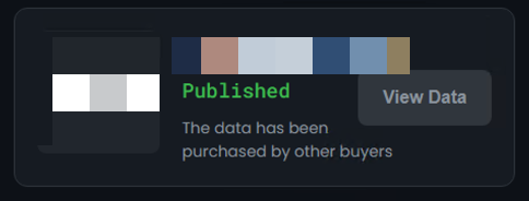
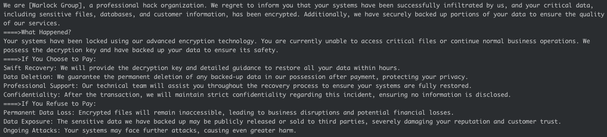
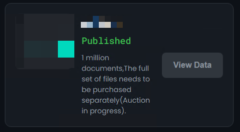
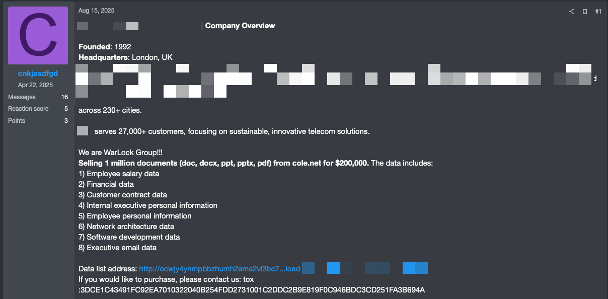

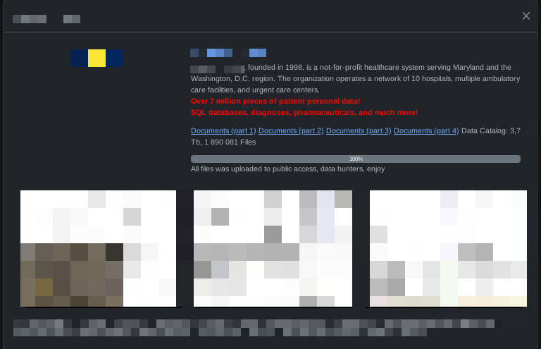
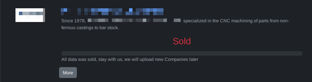
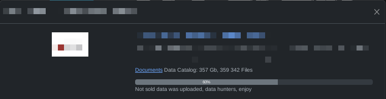
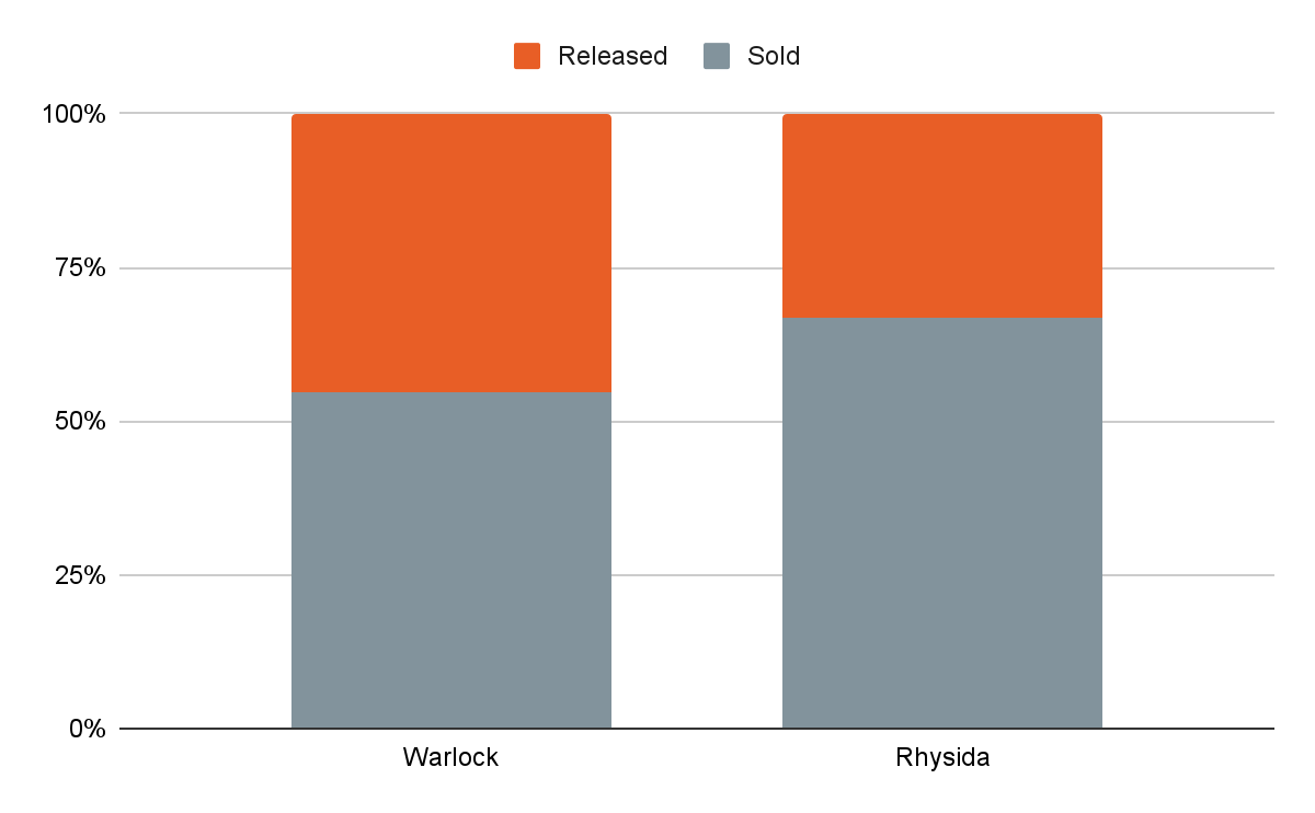
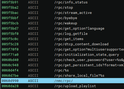
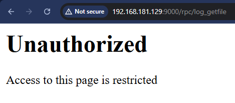
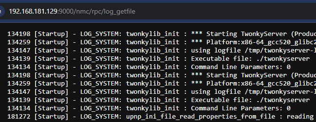
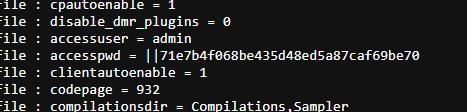
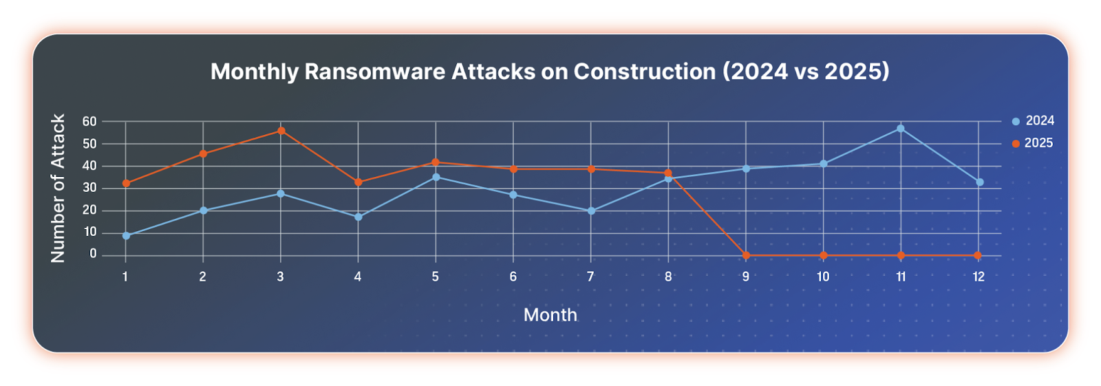
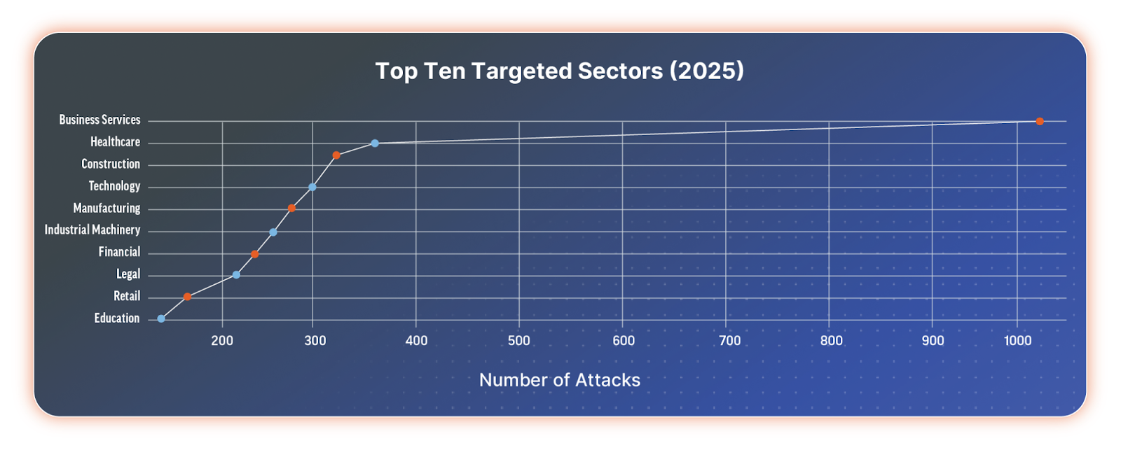
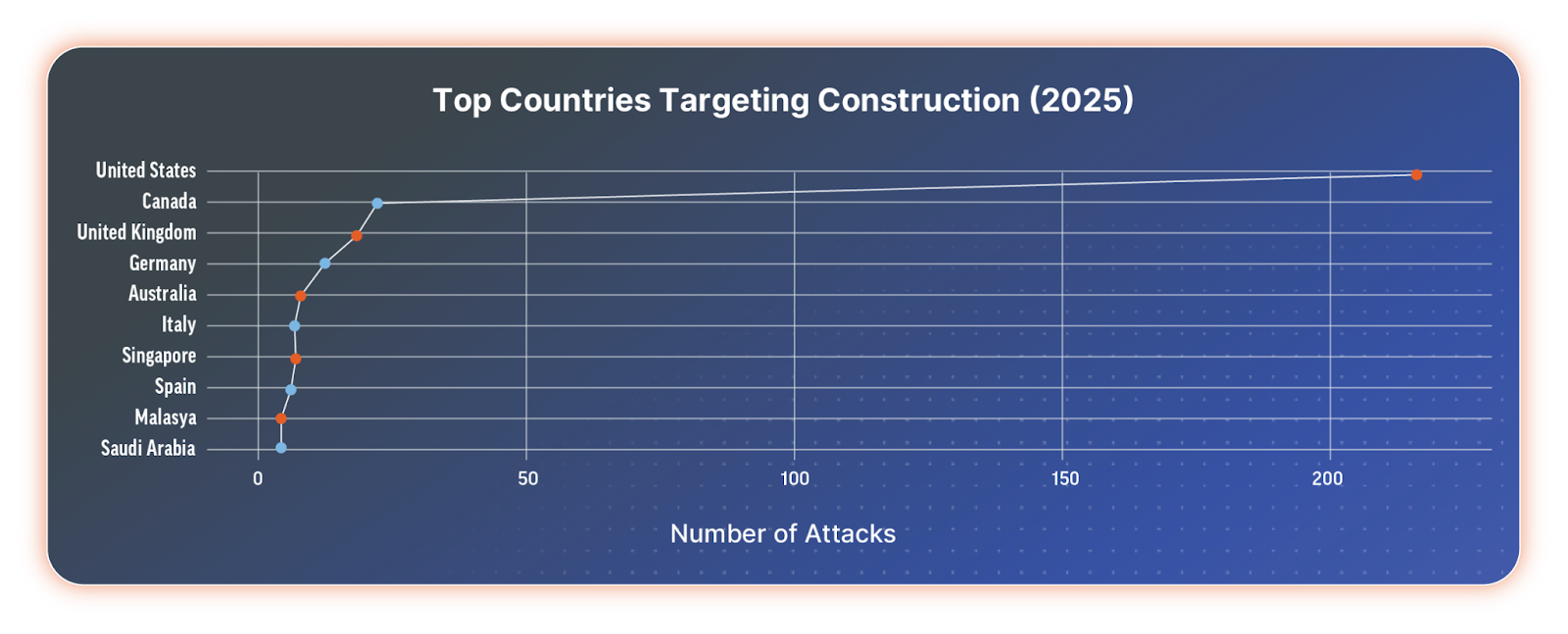
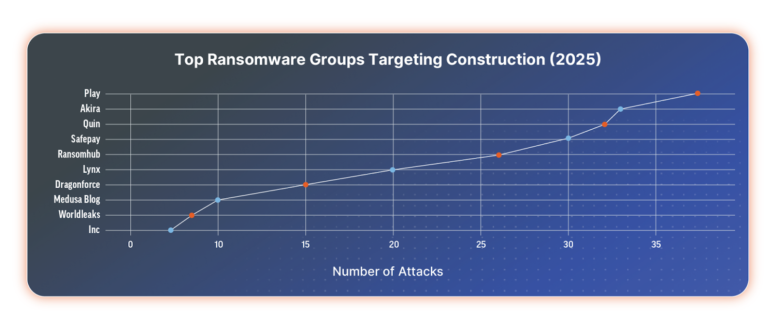
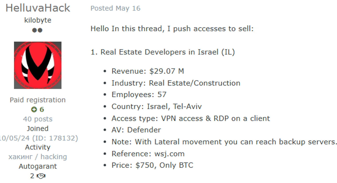
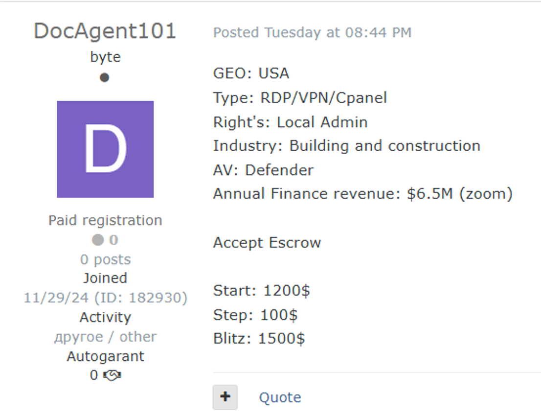


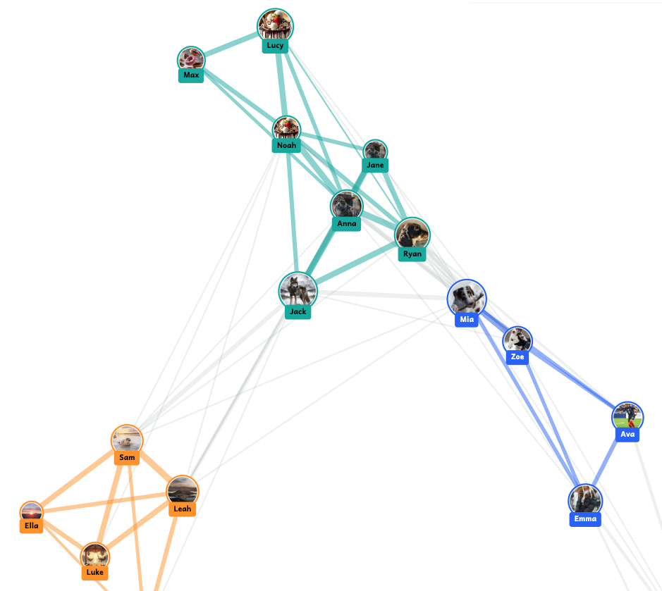
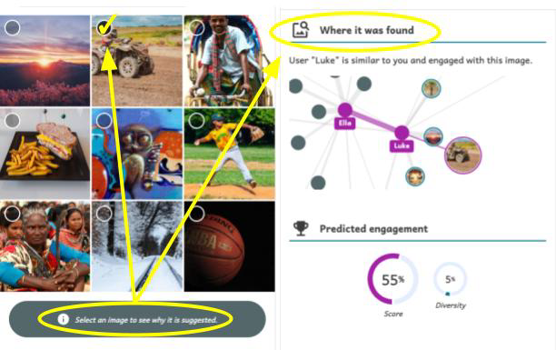


