Tag Archives: AWS Lambda

Implementing customer managed keys for AWS Lambda durable functions with Terraform

Post Syndicated from Rajdeep Banerjee original https://aws.amazon.com/blogs/compute/implementing-customer-managed-keys-for-aws-lambda-durable-functions-with-terraform/

If you run regulated workloads, you must control how persisted data is encrypted and who can access it. You need to manage encryption key rotation schedules, restrict decryption to authorized principals, and produce audit evidence that proves encryption controls are operating as designed.

AWS Lambda durable functions build resilient, multi-step workflows that survive failures through automatic checkpointing. The checkpoint mechanism persists execution state, including step results, payloads, and callback responses, to durable storage. For payment processing workloads, this persisted data is sensitive. AWS Lambda durable functions support customer managed keys from AWS Key Management Service (AWS KMS). A customer managed key gives you three controls: you set the key rotation schedule, you restrict decryption access through the key policy, and you generate per-function audit trails in AWS CloudTrail. A durable execution uses the same encryption key it started with for its entire lifetime. Changing or removing the key affects only executions that start after the change.

Updating the customer managed key policy to remove decrypt permissions, or disabling the key, stops the Lambda service from accessing previously checkpointed state. Customer managed key deletion is a permanent action, and all durable executions encrypted with that key become unrecoverable because the Lambda service has no mechanism to restore the data. Before scheduling key deletion, use the AWS KMS waiting period (7 to 30 days) and monitor AWS CloudTrail for Decrypt calls to confirm that the key is no longer in active use.

In this post, you learn to configure a customer managed key to encrypt durable execution data in an event-driven payment processing workflow. You create a symmetric encryption key in AWS KMS and define a key policy that grants the Lambda service, the function’s execution role, the function author, and durable execution operators only the AWS KMS actions each principal requires. You then configure the function to use the key for durable execution encryption and verify encryption operations through AWS CloudTrail logs. By the end, you have a deployable reference architecture you can adapt for regulated workloads running on Lambda durable functions.

To learn more about how AWS Lambda encrypts durable execution data, see Encrypting AWS Lambda durable execution data in the AWS Lambda Developer Guide.

Solution overview

The sample application implements an event-driven payment processing pipeline using Amazon DynamoDB, Amazon EventBridge, Amazon EventBridge Pipes, AWS Lambda, and Amazon SQS. The pipeline receives authorized payment transactions, validates and enriches them. A Lambda durable function applies business rules to the enriched transactions. The approved transactions are sent to a downstream settlement system for posting.

The following section covers the key architectural steps.

Architecture steps

  1. The upstream authorization system writes authorized payment records to a DynamoDB table.
  2. DynamoDB Streams captures each new record as an ordered change event.
  3. Amazon EventBridge Pipes polls the record from the DynamoDB stream. The pipe triggers a Lambda function as part of enrichment step for duplicate checking.
  4. The deduplication Lambda uses a DynamoDB table with conditional writes to identify duplicate inbound transactions based on transaction properties and time window.
  5. When the deduplication is successful, the pipe publishes an event to the Amazon EventBridge custom event bus.
  6. An Amazon EventBridge rule invokes a Lambda function for matching events. The function adds business context such as account type, bank routing details, and merchant category codes. The function publishes a new enriched event to the custom event bus.
  7. Another Amazon EventBridge rule matches the enriched events to a Lambda durable function. The durable function applies business rules to the incoming event. When the event passes all business rules, the function publishes a new event to the event bus.
  8. An Amazon EventBridge rule routes the approved event to an Amazon SQS queue preserving ordering for settlement and buffering against downstream throughput limits.
  9. The Posting Lambda function reads from the Amazon SQS and invokes the downstream posting subsystem to post the transaction. Finally, the function publishes a completion event to the event bus completing the transaction lifecycle.

With customer managed keys configured on DynamoDB, Amazon EventBridge, SQS, and the AWS Lambda durable function, every piece of persisted data in this pipeline is encrypted with keys you own and control. The walkthrough that follows shows you how to deploy this configuration with Terraform.

Figure 1 shows the reference architecture for this solution.

Reference architecture
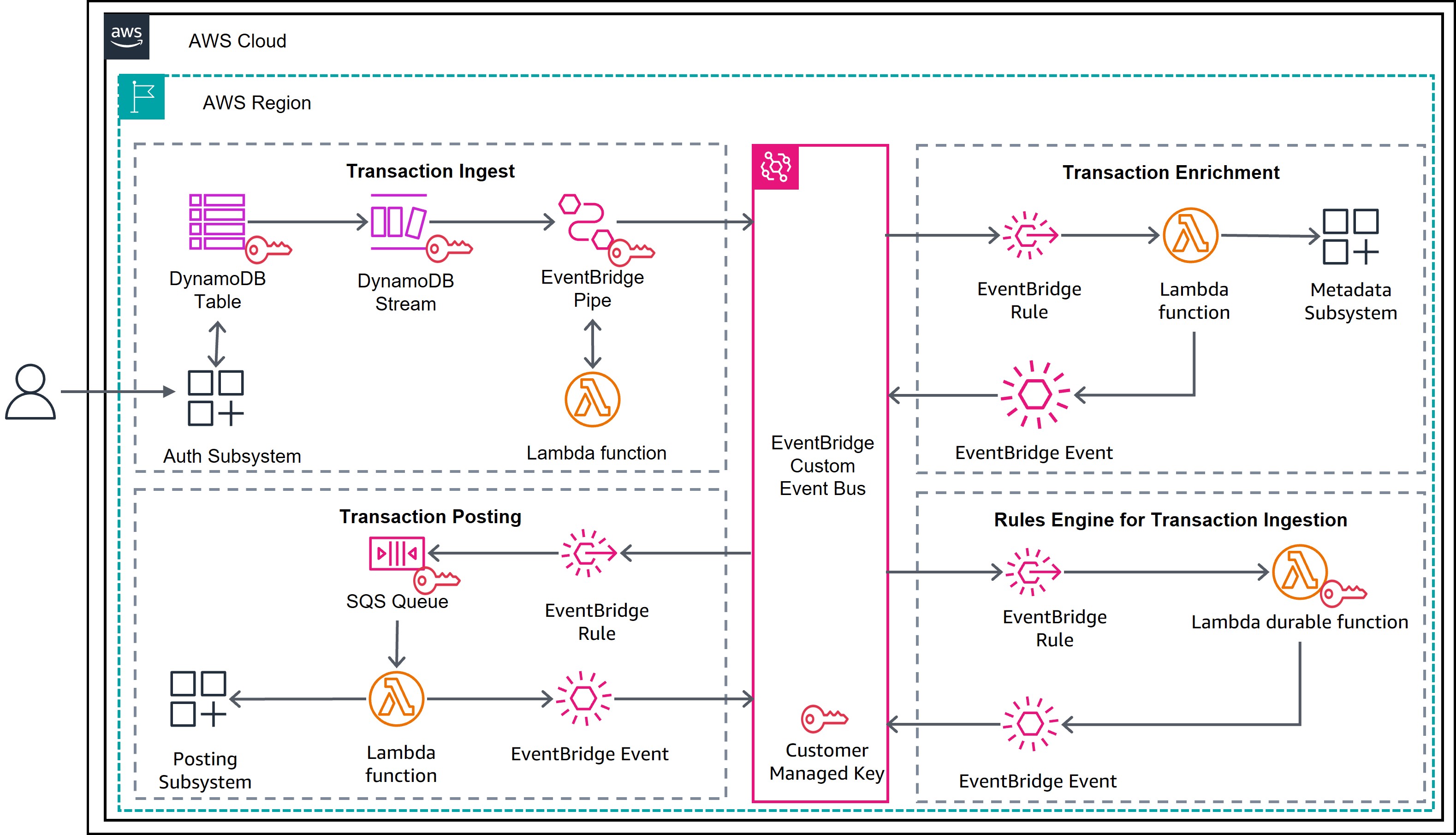
Reference architecture for payment processing using Lambda durable functions

Figure 1: Payment processing using Lambda durable functions

Prerequisites

To deploy this solution, you need the following prerequisites:

  1. AWS account and CLI: An active AWS account with the AWS CLI installed and configured with appropriate credentials.
  2. Terraform: Terraform installed (version 1.0 or later) for infrastructure provisioning.
  3. Python environment: Python 3.11 or later, with pytest for running unit tests. The aws-durable-execution-sdk-python package requires Python 3.11 or later.
  4. AWS Identity and Access Management (IAM) permissions: The IAM permissions to create the resources. Follow the sample repository for the sample policy.
  5. Basic understanding and familiarity with AWS Serverless services.

Solution walkthrough

The following is a step-by-step guide to deploy and test the payment processing solution.

Step 1: Clone the repository

git clone https://github.com/aws-samples/sample-payment-processing-with-lambda-durable-functions.git
cd sample-payment-processing-with-lambda-durable-functions/source

Step 2: Run unit tests

Validate the payment processing logic locally before deploying:

cd lambda-src/business_rules
pip3 install -r requirements-test.txt
pytest test_app.py -v

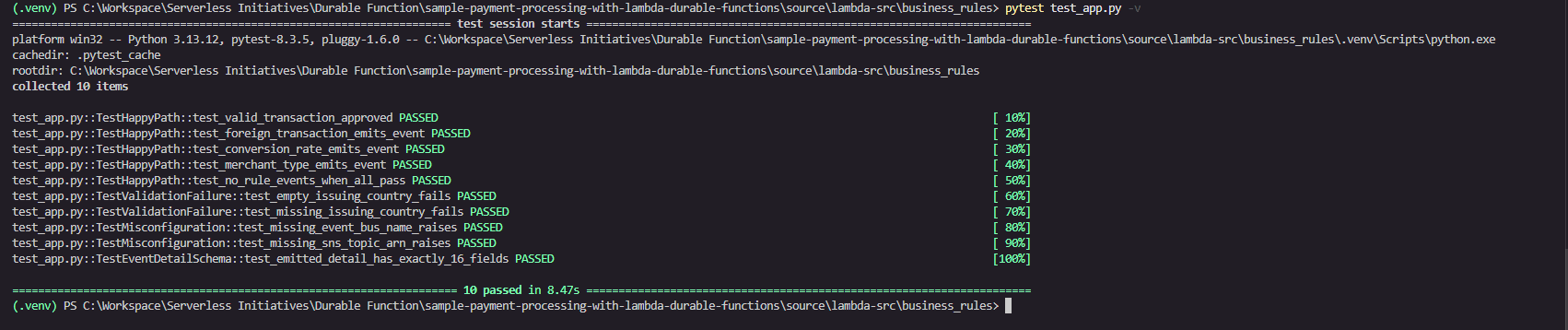
This runs unit tests that cover transaction validation, business rule checks (foreign transaction detection, currency conversion, merchant type), event schema validation, and misconfiguration handling. The tests use the AWS Durable Execution Testing SDK to run the handler locally without deploying AWS resources.

Figure 2 shows an example of test results running locally.
Test run results of the business rules

Figure 2: Test run results of the business rules

Step 3: Inspect the Lambda durable functions construct

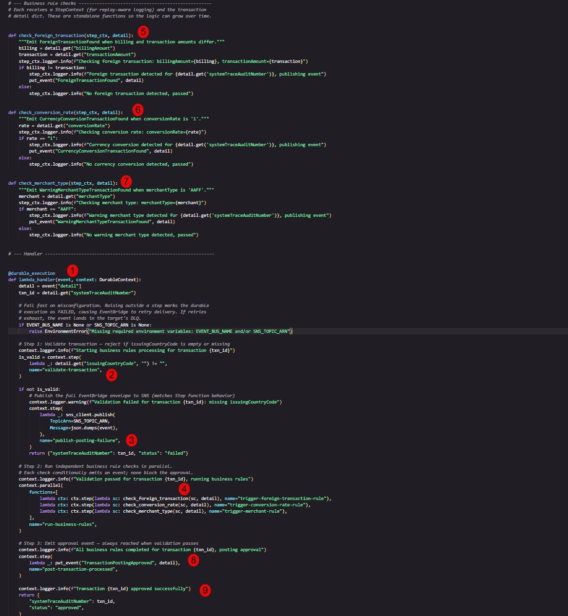
Open the payments-business-rules Lambda function in source/lambda-src/business_rules/business-rules-app.py for a sample Lambda durable function. Refer to Figure 3 for the code walkthrough.

Key features used

  1. @durable_execution decorator: Transforms a standard Lambda handler into a durable function handler. The durable execution SDK manages checkpointing automatically. No infrastructure changes are required.
  2. context.step("validate-transaction"): Validates that the transaction has a non-empty issuingCountryCode. The durable execution checkpoints the result (True or False) to durable storage. The durable execution restores checkpoint results instead of re-executing steps during the replay phase. This phase occurs whenever the function is re-invoked after an interruption such as a wait period completing, a failure, or a suspension. This checkpointed result is part of the durable execution data encrypted by your customer managed key.
  3. context.step("publish-posting-failure"): Publishes the full Amazon EventBridge envelope to Amazon SNS when validation fails. This step only runs on the failure path. The runtime checkpoints the Amazon SNS publish response to durable storage.
  4. context.parallel("run-business-rules"): Runs three independent rule checks concurrently: foreign transaction detection, currency conversion, and merchant type validation. Each branch checkpoints independently. If one branch fails, the others are not replayed on resume. Each branch result is persisted to durable storage and encrypted by the customer managed key.
  5. ctx.step("trigger-foreign-transaction-rule") (inside parallel): Compares billingAmount against transactionAmount. If they differ, it emits a ForeignTransactionFound event to Amazon EventBridge. This step is checkpointed independently within the parallel group.
  6. ctx.step("trigger-conversion-rate-rule") (inside parallel): Checks whether conversionRate equals 1. If so, it emits a CurrencyConversionTransactionFound event to Amazon EventBridge. This step is checkpointed independently within the parallel group.
  7. ctx.step("trigger-merchant-rule") (inside parallel): Checks whether merchantType equals AAFF. If so, it emits a WarningMerchantTypeTransactionFound event to Amazon EventBridge. This step is checkpointed independently within the parallel group.
  8. context.step("post-transaction-processed"): Emits the final TransactionPostingApproved event to Amazon EventBridge. This step is only reached when validation passes and all business rules complete. The runtime checkpoints the Amazon EventBridge response. On replay, if this step already succeeded, the event is not re-published, which guarantees exactly-once approval semantics.
  9. context.logger: Provides replay-aware logging throughout the handler. During replay of previously completed steps, log statements are suppressed to prevent duplicate log entries in Amazon CloudWatch.
Lambda durable functions code walkthrough

Figure 3: Sample Lambda durable functions code

Step 4: Deploy infrastructure with Terraform

Terraform currently doesn’t support attaching a customer managed key directly to the durable function. You create the symmetric key in Terraform and then associate the key with the durable function on the AWS Management Console. Refer to source/durable_kms.tf for the key configuration.

Initialize and deploy the AWS resources that make up the solution:

cd ../../
terraform init
terraform plan -var="region=us-east-2"

Review the plan output, then apply:

terraform apply -var="region=us-east-2" --auto-approve

Note: Replace us-east-2 with your preferred AWS Region.

On successful completion, Terraform outputs the AWS KMS key alias, key ARN, and DynamoDB Streams ARN used by the event-driven pipeline:

Apply complete! Resources: N added, 0 changed, 0 destroyed.

Outputs:

durable_kms_key_alias = "durable-function-encryption"
durable_kms_key_arn = "arn:aws:kms:us-east-2:xxxxxxxxxxxx:key/4e87d4c2-1190-4db4-8b97-46657f83ee00"
stream_arn = "arn:aws:dynamodb:us-east-2:xxxxxxxxxxxx:table/visa/stream/2026-03-16T14:25:47.847"

Step 5: Verify Lambda durable functions configuration

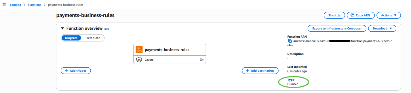
In the AWS Lambda console, navigate to the payments-business-rules function. Confirm that the function Type displays Durable, which indicates that the checkpoint-and-replay mechanism is active. Figure 4 shows the expected function configuration.
The durable function in the AWS Lambda console

Figure 4: The Lambda durable function in the AWS Lambda console

Step 6: Add the AWS KMS key to the Lambda durable function

  1. The durable function is not encrypted with a customer managed key. Figure 5 shows the function’s encryption configuration as empty.

    The Lambda durable function missing an AWS KMS key in the AWS Lambda console

    Figure 5: The Lambda durable function missing a customer managed key in the AWS Lambda console
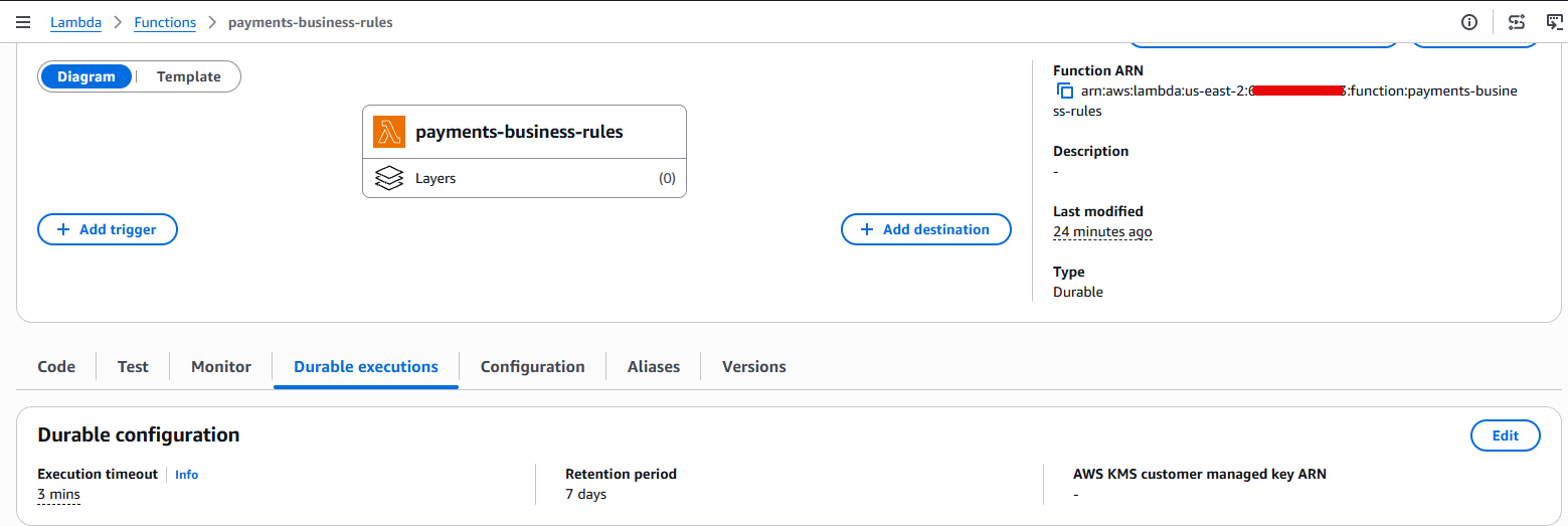
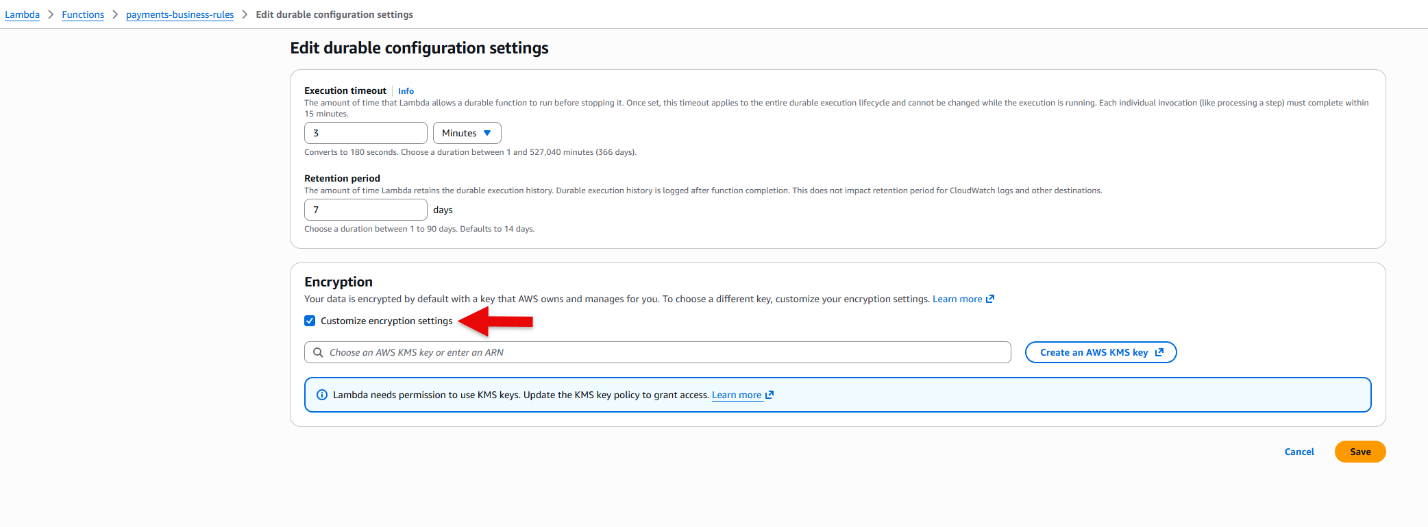
  2. Choose Edit, then turn on Customize encryption settings as shown in Figure 6.

    The Lambda durable function encryption settings in the AWS Lambda console

    Figure 6: The Lambda durable function check encryption in the AWS Lambda console

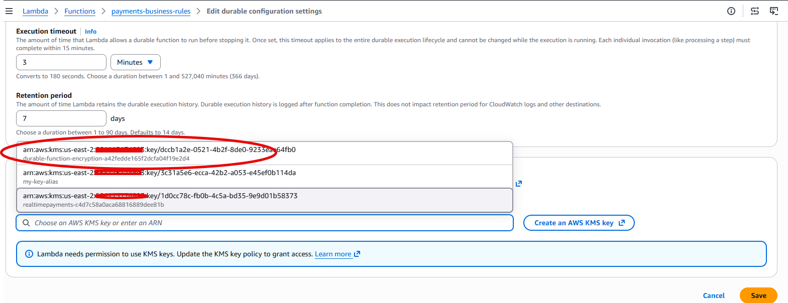
  3. Select the AWS KMS key ARN created for the durable function. The key ARN is available in the Terraform output from Step 4. Figure 7 shows the key selection.

    Selecting the AWS KMS key for the durable function in the AWS Lambda console

    Figure 7: Select the AWS KMS key ARN for the durable function in the AWS Lambda console

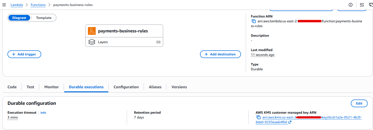
  4. Choose Save and confirm that the durable function is now encrypted with a customer managed key, as shown in Figure 8.

    The Lambda durable function with the AWS KMS key in the AWS Lambda console

    Figure 8: AWS Lambda durable function with the customer managed key in the AWS Lambda console
Step 7: Execute a test payment

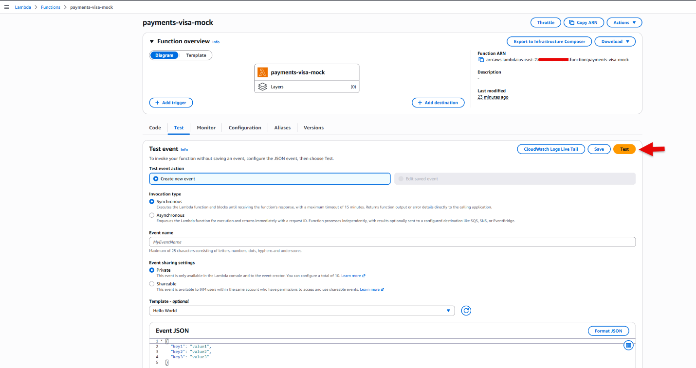
Invoke the payments-visa-mock Lambda function to simulate an end-to-end authorization flow. The mock function reads sample Visa authorization messages from a CSV file and writes them to DynamoDB, which triggers the event-driven pipeline. Figure 9 shows a sample test invocation.
Invoking the payments-visa-mock function to trigger the workflow

Figure 9: Invoke the payments-visa-mock function to trigger workflow

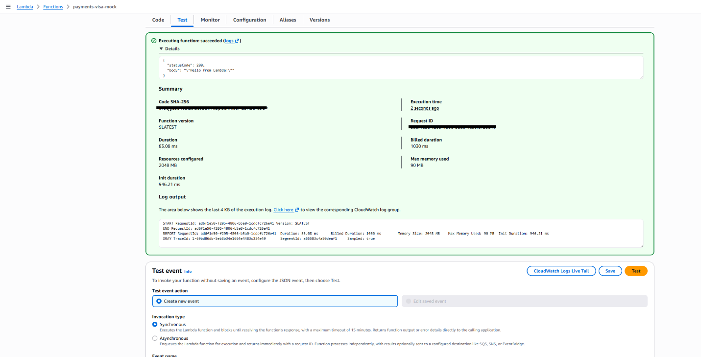
Figure 10 shows a sample response after invocation.
Test results from the payments-visa-mock function

Figure 10: Test results from the payments-visa-mock function to trigger workflow

The mock Lambda invocation creates records that follow the process described in the preceding architecture steps.

Step 8: Verify results

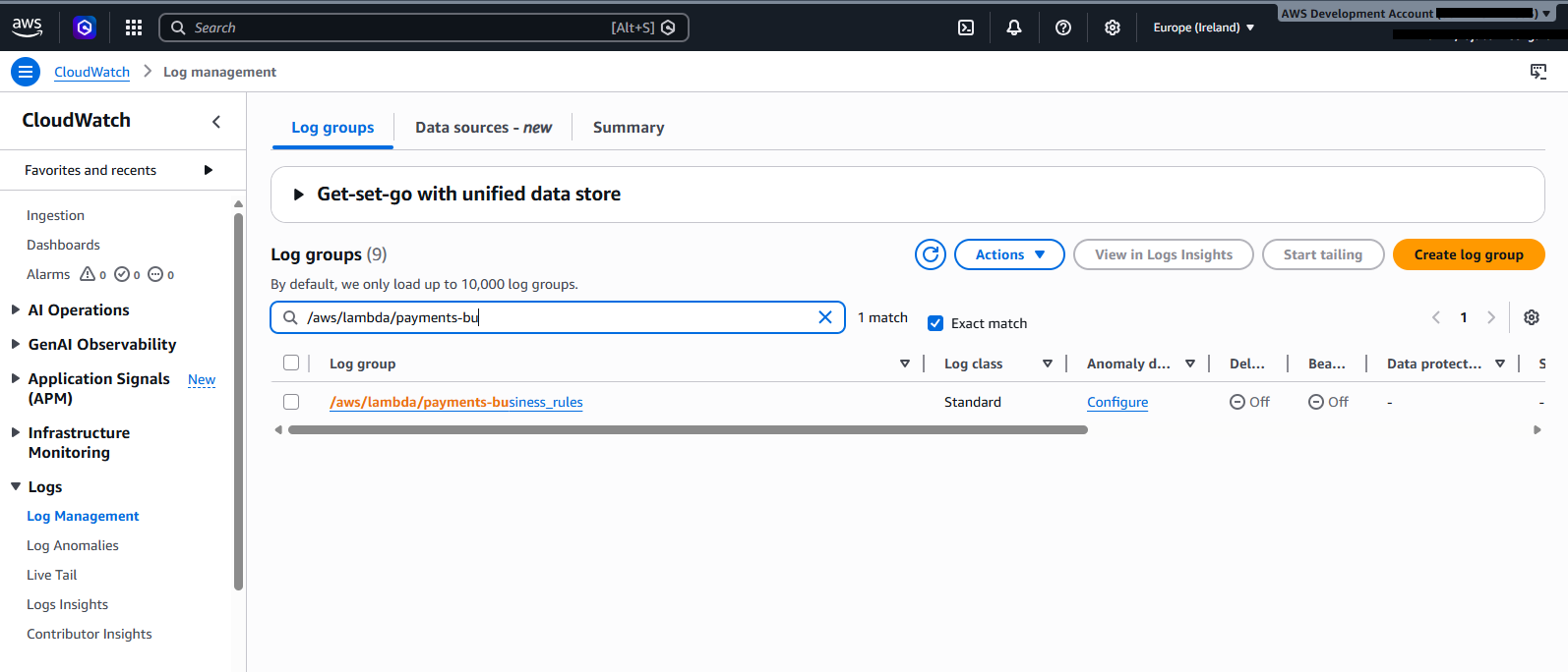
Open Amazon CloudWatch Logs and inspect the log group /aws/lambda/payments-business_rules. This log group belongs to the Lambda durable function for this use case. Figure 11 shows the CloudWatch log group on the console.
Search in CloudWatch Logs for the durable function log group

Figure 11: Search in CloudWatch

You see the complete business rules lifecycle for each transaction, as shown in Figure 12. The highlighted sections show all the business rules performed by the durable function. Each step is checkpointed by the runtime and encrypted by the customer managed key.
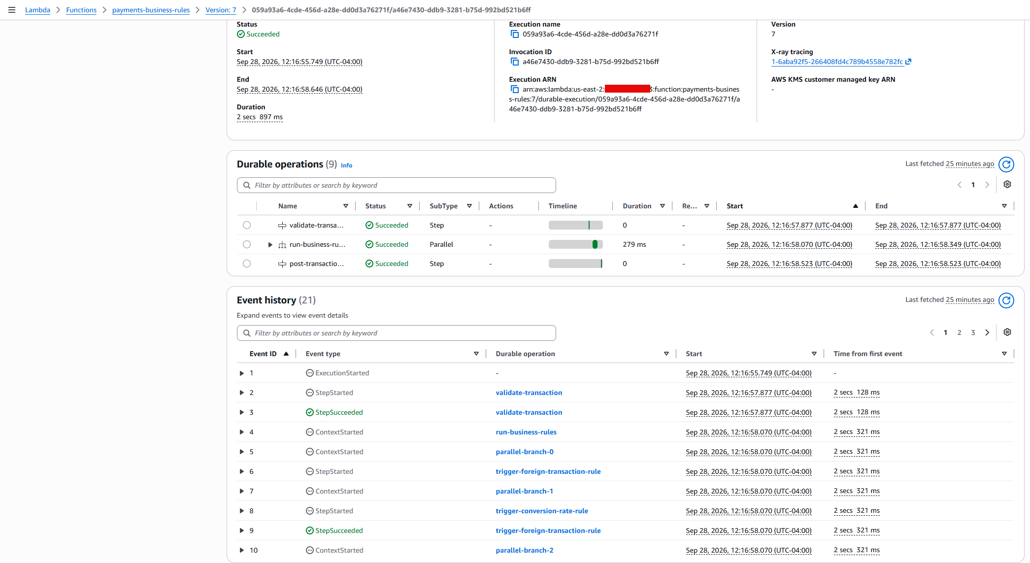
Search Results in lambda durable functions console

Figure 12: Search Results in lambda durable functions console

You can also check the other log groups to trace the full pipeline:

  • /aws/lambda/payments-enrich: Transaction enrichment logs.
  • /aws/lambda/payments-posting: Settlement posting logs.

Step 9: Verify the customer managed key configuration

You can verify the key configuration by using the AWS CLI:

aws lambda get-function-configuration \
    --function-name payments-business-rules \
    --query "DurableConfig" \
    --region us-east-2

Expected response:

{
    "KMSKeyArn": "arn:aws:kms:us-east-2:xxxxxxxxxxxx:key/4e87d4c2-1190-4db4-8b97-46657f83ee00",
    "RetentionPeriodInDays": 7,
    "ExecutionTimeout": 180
}

You can search in AWS CloudTrail to track the AWS KMS calls. When you configure or update the customer managed key on a durable function, Lambda validates the key policy with dry-run GenerateDataKey and Decrypt calls. These appear in CloudTrail with a DryRunOperationException error code, which confirms that the key policy permissions are correct and does not indicate an actual error. For more details, see Encrypting AWS Lambda durable execution data.

Clean up

To avoid ongoing charges, destroy all deployed resources using the following command:

terraform destroy -var="region=us-east-2" --auto-approve

Expected output:

Destroy complete! Resources: N destroyed.

Conclusion

In this post, you configured a customer managed key to encrypt durable execution data in a Lambda durable function. With a customer managed key, you control the key rotation schedule, restrict decryption access through the key policy, and generate per-function audit trails in AWS CloudTrail. You can revoke access to durable execution data at any time by updating the key policy, giving you full control over who can read execution state. In-flight executions stop at the next checkpoint call and new executions must be started after restoring access. For details, see When the customer managed key is unavailable.

For payment processors and financial institutions, encrypting durable execution data with a customer managed key satisfies compliance obligations for data-at-rest encryption, key governance, and access auditability across multi-step transaction workflows.

To get started, clone the sample repository and follow the preceding walkthrough. To learn more about Lambda durable functions, see the AWS Lambda Developer Guide.

Improving Lambda function latency with scalable network bandwidth

Post Syndicated from Rahul Shandilya original https://aws.amazon.com/blogs/compute/improving-lambda-function-latency-with-scalable-network-bandwidth/

AWS Lambda now supports scalable network bandwidth for functions configured with 2,048 MB of memory or more, running outside of a virtual private cloud (VPC). Previously, sustained network throughput was capped at 625 Mbps regardless of your function’s memory configuration. Now, sustained throughput scales proportionally from 625 Mbps at configurations below 2,048 MB up to 3,000 Mbps at 10,240 MB, increasing the rate at which data moves to and from your execution environment.

In this post, you learn how to apply this new capability to latency-sensitive data processing workloads, helping reduce function execution times and per-invocation costs while improving the end-user experience through reduced latency. You also walk through a deployable implementation that demonstrates the performance improvements this capability unlocks.

Latency-sensitive data processing

Latency-sensitive data processing applications are data processing workloads that must be completed in a defined period of time. They often experience bursty, ad hoc traffic patterns while being required to download gigabytes or even terabytes of data from a data store, process it in a compute environment, and return a result to a waiting end user.

Latency-sensitive data processing is often highly parallelizable. Data can be divided into smaller pieces with each piece being individually processed before combining them together to obtain a result.

These workloads can be found in multiple industries and verticals. Examples include:

  • Log querying engines – An end user initiates an on-demand search across terabytes of log data and expects results within seconds.
  • Insurance underwriting – A prospective customer submits an application, triggering real-time evaluation of historical claims and risk data. The underwriting process determines what coverage and premiums to offer to the prospective customer.
  • Financial ETL pipelines – An economic announcement triggers an unexpected burst of market data that must be ingested, transformed, and made available to downstream trading systems before the next market tick.
  • Genomics platforms – A clinician orders a diagnostic test, requiring gigabytes of DNA or RNA sequencing data to pass through a bioinformatics pipeline and be compared against a reference genome while the patient awaits results.

These workloads are challenging to build on traditional compute clusters. Their spiky and unpredictable nature forces you to choose between under-provisioning compute to optimize costs (and risk missing your SLA) or over-provisioning and paying for idle capacity.

Why Lambda fits latency-sensitive data processing

Lambda eliminates this tradeoff. Instead of pre-provisioning a compute cluster, Lambda scales compute capacity in response to incoming requests, matching processing power to unpredictable traffic patterns. Because latency-sensitive data processing is highly parallelizable, the ability of Lambda to rapidly scale out execution environments makes it a natural fit. You can fan out across thousands of concurrent functions to process data in parallel, paying only for the compute you use.

However, as data volume and performance requirements grow, network bandwidth to and from the compute environment can become the limiting factor in minimizing workload latency.

Scalable network bandwidth directly addresses this limitation by raising the per-environment network throughput ceiling, improving the rate at which data can be transferred to and from the execution environment. Each execution environment can now drive up to 3,000 Mbps of sustained throughput when configured with 10,240 MB of memory, a 4.8x increase from the previous ceiling of 625 Mbps. Combined with the ability of Lambda to scale out at a rate of 1,000 execution environments every 10 seconds, you can download more than 3 TB of data in under 10 seconds.

New network throughput behavior for Lambda functions

Scalable network bandwidth applies to both data ingress to and egress from an execution environment for functions outside of a VPC. For functions configured with 2 GB of memory or more, network bandwidth scales by approximately 280 Mbps increments for every 1 GB of additional memory allocated.

The following table shows the maximum sustained bandwidth available to each execution environment at each memory configuration.

Memory Configuration Max Sustained Bandwidth
Less than 2,048 MB 625 Mbps
2,048 MB 765 Mbps
3,072 MB 1,044 Mbps
4,096 MB 1,324 Mbps
5,120 MB 1,603 Mbps
6,144 MB 1,883 Mbps
7,168 MB 2,162 Mbps
8,192 MB 2,441 Mbps
9,216 MB 2,721 Mbps
10,240 MB 3,000 Mbps (4.8x increase)

Table 1. Lambda sustained network bandwidth by memory configuration. Bandwidth scales at ~280 Mbps per additional GB of memory above 2 GB.

In the following section, you learn how scalable network bandwidth improves end-user latency by building an ETL pipeline that demonstrates it. You can find the source code in the GitHub repository.

Solution overview

Consider a SaaS analytics platform where users submit ad hoc queries against a data store. The application must extract the relevant data, apply a filter or transformation, and return an aggregate result while the user waits. In this example, the result needs to be returned in 8 seconds or less.

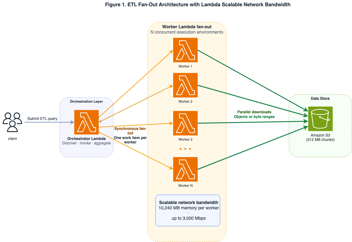
The following diagram illustrates the architecture of the solution.

ETL fan-out architecture: a client calls an orchestrator Lambda function, which fans out to multiple worker Lambda functions that read data in parallel from Amazon S3, with bandwidth scaling callouts for each memory tier.

Figure 1. ETL fan-out pattern: an orchestrator Lambda function distributes work to multiple worker Lambda functions that read from Amazon S3 in parallel, with bandwidth scaling callouts per memory tier.

A client initiates an ad hoc query by calling the orchestrator Lambda function through the Lambda API. The orchestrator function determines how to split the work. To process the data in parallel, the orchestrator function uses a ThreadPoolExecutor to issue synchronous invoke requests to the Lambda worker function, fanning out the worker across multiple execution environments at the same time.

Each Lambda worker function is configured with 10,240 MB of memory, so it has access to up to 3,000 Mbps of sustained network throughput. After the data is processed, the aggregated result is returned to the client.

Prerequisites

Before you start the deployment process, make sure that you have completed the following steps:

  1. Install the AWS SAM CLI on your computer and confirm that you are running Python 3.12 or later.
  2. Have your AWS account credentials ready.
  3. Submit a request to AWS Service Quotas to turn on scalable network bandwidth for your Lambda functions. This quota is listed under Network bandwidth per execution environment.

Clone the source code from the GitHub repo and deploy the application within your AWS account. Creating the 10 GB test dataset and running the benchmark can incur charges to your AWS account.

git clone https://github.com/aws-samples/sample-lambda-enhanced-bandwidth
cd sample-lambda-enhanced-bandwidth
sam build
sam deploy --guided

After the AWS CloudFormation stack is deployed, record the DataBucketName and orchestrator function name from the stack outputs to use in subsequent commands.

To simulate data for the end user to query, the GitHub repo has a script that creates 10 GB of synthetic data and uploads it to your S3 bucket.

Mode 1: Processing pre-partitioned data

In Mode 1, the 10 GB of synthetic data is pre-partitioned. Pre-partitioned data is typically produced incrementally by many sources over a period of time, which can be the case with IoT data or access logs. The following command creates 10 GB of data divided into 20 partitions that are 512 MB each.

python scripts/generate_data.py \
    --bucket <DATA_BUCKET_NAME> \
    --total-gb 10 \
    --chunk-mb 512

Turning on scalable network bandwidth does not, on its own, make your downloads faster. A single download request only opens one connection to Amazon S3, and one connection does not move data fast enough to fill all the bandwidth now available to your Lambda function. To actually use your full allotment of network bandwidth, the execution environment has to pull the data over several connections at once. It does this by preferring the AWS Common Runtime (CRT) transfer client, a high-performance download engine built into Boto3. When the worker calls download_fileobj, the CRT client automatically breaks the 512 MB object into smaller parts and downloads them in parallel across multiple Amazon S3 requests. Those parallel downloads are what let a single Lambda worker take advantage of its full network bandwidth.

The following command runs the benchmark on the pre-partitioned data.

python scripts/run_fanout_benchmark.py \
    --orchestrator-name <STACK_NAME>-orchestrator \
    --bucket <DATA_BUCKET_NAME> \
    --iterations 5

Mode 2: Processing single large objects

Mode 2 generates 10 GB of data in one large object. This arrangement is more common when data is produced or delivered as one complete unit, such as database backups or genomic datasets. The following command creates 10 GB of data in a single large object.

python scripts/generate_data.py \
    --bucket <DATA_BUCKET_NAME> \
    --single-object-gb 10 \
    --key large-object/large-file.bin

In Mode 1, the CRT preference applies to Boto3 managed transfer methods such as download_file and download_fileobj. Mode 2 takes a different approach. Each worker reads a specific byte range of a single large object using get_object. The CRT preference setting has no effect on these calls. Instead, you can control concurrency by explicitly tuning the number of Lambda workers and using a bounded ThreadPoolExecutor to issue multiple byte-range requests at the same time.

When you run the following command, the orchestrator takes the single large object and divides it into consecutive byte ranges of 512 MB each. Each of the individual ranges is then processed by a Lambda worker execution environment in parallel.

python scripts/run_fanout_benchmark.py \
    --orchestrator-name <STACK_NAME>-orchestrator \
    --bucket <DATA_BUCKET_NAME> \
    --key large-object/large-file.bin \
    --slice-size-mb 512 \
    --iterations 5

The benchmark reports wall-clock duration, client-observed duration, aggregate throughput across workers, worker completion counts, and target compliance. When comparing memory configurations, keep the code, dataset, AWS Region, partition count, warm-up policy, and measurement count identical. You should run the benchmark multiple times in your account because placement, cold starts, concurrency, S3 behavior, and execution-environment reuse could affect results.

Results

To compare results, we ran the benchmark using a baseline configuration where the worker Lambda function is configured with only 1,024 MB of memory, well below the 2,048 MB threshold required for scalable network bandwidth to take effect. The 1,024 MB configuration limits network throughput to the previous sustained ceiling of 625 Mbps.

In our baseline test run, a worker downloaded and processed a single 512 MB partition with a 6.61-second download time at a 649.8 Mbps throughput (at p50). The 649.8 Mbps throughput exceeds the 625 Mbps ceiling because Lambda is capable of bursts in network throughput over a short period of time. Across twenty measured fan-out queries, the complete 10 GB query was completed with a 7.113-second wall-clock at p50. This fits within the 8-second SLA but leaves very little headroom.

To run our scalable network bandwidth benchmark, we re-deployed our worker Lambda function with a 10,240 MB memory configuration and re-ran the application. At a 10,240 MB memory configuration, each execution environment can now access up to 3,000 Mbps in sustained throughput. Direct 512 MB downloads achieved a 1.70-second download time and 2,521.3 Mbps throughput (both at p50). The complete 10 GB query was completed with a 2.640-second wall-clock at p50. That is 2.69 times faster, or 62.9% lower median latency, than the 1,024 MB configuration.

Table 2 summarizes the direct worker and end-to-end fan-out measurements for the same 10 GB dataset and 20 × 512 MB orchestration pattern. Aggregate throughput is the total data transfer rate across all twenty execution environments spun up to run the benchmark.

Memory Configuration Single 512 MB partition download time and throughput (p50) 10 GB fan-out wall time (p50) Aggregate throughput p50
1,024 MB baseline tier (sustained 625 Mbps) 6.61s / 649.8 Mbps 7.113s 12.08 Gbps
10,240 MB scalable tier (up to 3,000 Mbps) 1.70s / 2,521.3 Mbps 2.640s 32.54 Gbps

Table 2. Measured 1,024 MB baseline tier and 10,240 MB scalable bandwidth performance for a 10 GB fan-out ETL query.

Using scalable network bandwidth, the customer’s SLA headroom has improved by nearly 5 seconds. The Lambda function can now handle larger partitions within the same SLA window, reducing costs while still remaining comfortably within the customer’s SLA.

Clean up

To clean up the resources you created for the benchmark test, run the following commands:

aws s3 rm s3://<DATA_BUCKET_NAME> --recursive
sam delete --stack-name <STACK_NAME>

Best practices

After scalable network bandwidth is turned on for your AWS account, the following practices help you get the most out of it.

Profiling and planning

  • Test before you tune. Not every function is network-bound. Before increasing memory, profile your function to confirm that network I/O is the primary contributor to invocation duration and not CPU or application logic. Use Amazon CloudWatch Lambda Insights to inspect rx_bytes, tx_bytes, and duration. Functions where network I/O dominates invocation time are prime candidates for tuning.
  • Design for parallelism. Break your data into parallelizable chunks that can be processed independently in a fan-out pattern across multiple execution environments. You can use Amazon S3 byte-range reads to split large files into independently downloadable partitions. For implementation details, see Downloading an object with part numbers in the Amazon S3 User Guide.
  • Run AWS Lambda Power Tuning. Lambda Power Tuning is a state machine that helps you optimize your Lambda functions for cost and performance. Use Power Tuning to sweep memory configurations from 1,024 MB to 10,240 MB and identify the optimal cost-vs-latency point for your workload.

Implementation

  • Check upstream and downstream limits. Check the throughput limits of your data sources. For example, a Lambda function running at 3,000 Mbps can exceed the throughput capacity of a single S3 prefix, which supports up to 5,500 GET requests per second. When this happens, you will see HTTP 503 (Slow Down) errors in your application logs. Distribute your S3 objects across multiple prefixes to parallelize reads and avoid per-prefix throttling.
  • Balance bandwidth and CPU. Lambda allocates CPU proportionally to memory. For example, at a 1.7 GB memory configuration you are allocated 1 vCPU while a 10 GB memory configuration is allocated up to 6 vCPU. If your function processes data in parallel threads, the higher memory tiers give you both more network bandwidth and more CPU to process it. Use the concurrent.futures module in Python or worker_threads in Node.js to process data across parallel threads and maximize both CPU and network utilization.
  • Turn on Amazon S3 CRT for Boto3. If your function uses the Python runtime, initialize your Amazon S3 client with preferred_transfer_client: 'crt' to maximize single-connection throughput. The AWS Common Runtime automatically parallelizes requests across multiple TCP connections, which matters because individual TCP connections have a throughput ceiling.
  • Use SnapStart for JVM workloads. If you use Lambda SnapStart for Java functions, scalable network bandwidth reduces afterRestore hook latency. Network activity that occurs during function restore, such as pre-warming connections or pre-fetching configuration data, can complete faster.

Conclusion

Scalable network bandwidth raises the per-environment sustained throughput ceiling of AWS Lambda from 625 Mbps to 3,000 Mbps, directly reducing end-to-end latency for data-intensive workloads. Combined with the Lambda scaling rate, you can now move terabytes of data in seconds, without provisioning or managing infrastructure.

To get started, request the Network bandwidth per execution environment quota increase through AWS Service Quotas and deploy the sample application from the GitHub repository to see the improvement firsthand.

AWS Weekly Roundup: GPT-6 Sol and Luna, Claude Opus 5.5 on Amazon Bedrock, Strands harness, and more (September 28, 2026)

Post Syndicated from Daniel Abib original https://aws.amazon.com/blogs/aws/aws-weekly-roundup-gpt-6-sol-and-luna-claude-opus-5-5-on-amazon-bedrock-strands-harness-and-more-september-28-2026/

If there’s one theme that defined last week, it’s choice. The frontier models keep arriving, and the interesting question is no longer just “how smart is it?” but “which model fits this step, at this cost, at this latency?” That’s exactly what landed on Amazon Bedrock over the past few days: GPT-6 Sol and GPT-6 Luna from OpenAI, giving you two new points on the intelligence-versus-efficiency curve, and Claude Opus 5.5 from Anthropic, the first of the Claude 5.5 family.

GPT-6 Sol is built for the demanding, recurring work of development and operations, while GPT-6 Luna makes focused, repeatable tasks practical at high volume, and both ship at significantly lower pricing than their GPT-5.6 predecessors. Claude Opus 5.5, meanwhile, does more with fewer tokens than Opus 5 and is tuned for agentic coding and long-running tasks. What I like about all three is that they push toward the same idea: match the model to the job instead of reaching for the biggest one every time. The other thread was observability catching up to this agentic world, including a launch I had the pleasure of writing about myself.

Now, let’s get into this week’s AWS news…

Last week’s launches

Here are some launches and updates from this past week that caught my attention:

  • Introducing Amazon CloudWatch Omni – You can now observe your applications and AI agents together in a single, collaborative experience. Amazon CloudWatch Omni is built on OpenTelemetry, so your existing telemetry shows up with nothing to reconfigure, and your whole team reaches it through one URL with enterprise SSO — no console access required. It auto-discovers your services, maps dependencies, and brings AWS DevOps Agent into investigation sessions to correlate signals and trace root causes. There’s a companion post on the agent-observability side, a deeper dive on the AWS Cloud Operations blog on what observability for the AI era looks like, and the announcement on What’s New with the specifics. If you want the bigger picture, Matt Wood’s Wrong, not broken is a great read on why correctness now has to be measured at the level of the run.
  • Enhanced custom event buses in Amazon EventBridge – Amazon EventBridge now offers an enhanced custom event bus purpose-built for organizations scaling event-driven applications across teams and accounts. You can now deploy a single centralized bus shared across every account in your organization through AWS RAM, with optional event ordering, a simplified Subscriber resource that bundles filtering, targets, and retries, content-based deduplication, and synchronous invocation for targets like AWS Lambda. A new ingress/egress pricing model replaces the compounding cross-account routing charges of multi-bus setups, and your existing buses keep working unchanged as “classic.”
  • Amazon SageMaker HyperPod Inference Gateway – You can now front your LLM inference on Amazon SageMaker HyperPod with a Kubernetes-native, GPU-aware routing layer that deploys as a single Amazon EKS managed add-on with zero application changes. Instead of round-robin load balancing, it routes on real-time inference signals — KV cache utilization, queue depth, prefix cache hits, predicted latency, and more — cutting first-token latency by up to 82% in mixed-hardware and bursty scenarios. It works with any OpenAI-compatible model server, including vLLM and SGLang.
  • AI agent skills for AWS End User Messaging and Amazon SES – You can now build and send messages by asking your AI coding agent in plain language. Amazon SES and AWS End User Messaging publish AI agent skills for the AWS MCP Server, giving your agent step-by-step, validated guidance for tasks like verifying a sending identity, sending a production email, or building a branded RCS agent with cards and buttons. The skills work with Claude Code, Codex, Cursor, and Kiro, so you can complete messaging workflows without hopping between docs and console screens.

For a full list of AWS announcements, be sure to keep an eye on the What’s New with AWS page.

Other AWS news

Here are some additional posts and resources that you might find interesting:

  • Introducing Strands harness – The Strands Agents team released Strands harness, a fully assembled, general-purpose agent harness you can run locally or deploy anywhere, under Apache 2.0. It takes one line of Python or TypeScript to wire up your model of choice across Amazon Bedrock, Anthropic, OpenAI, Google, or a local Ollama model, and it ships with sensible defaults for prompt caching and context management (truncating bulky tool results, compacting when the context window fills up, and keeping memory across runs). The team reports it costs about 28% less than comparable harnesses on the same models while holding accuracy steady.
  • Announcing the new AWS Reimagine report on AI – The AWS Executive in Residence team spent nine months interviewing 154 leaders across 27 countries about what separates organizations that turn AI into value from those that don’t. The report is candid (including where AI hasn’t worked at Amazon), and the recurring insight is that once building gets fast, the bottleneck moves to deciding, funding, and governing the work. Well worth a read if you’re thinking about how your teams adopt AI in practice.

For a full list of AWS blog posts, be sure to keep an eye on the AWS Blogs page.

Upcoming AWS events

Check your calendar and sign up for upcoming AWS events:

  • AWS re:Invent – AWS re:Invent returns to Las Vegas from November 30 to December 4, and session times, locations, and speakers are live. Reserved seating opens October 6, so register now and be ready to claim your spot in chalk talks, workshops, and builders’ sessions.
  • AWS Summits – With re:Invent on the horizon, the Summits are wrapping up for the year. The last stop is Dubai (September 30) at the Dubai World Trade Center, with 60+ sessions, an AWS Village, and hands-on workshops.
Join the AWS Builder Center to connect with builders, share solutions, and access content that supports your development. Browse here for upcoming AWS-led in-person and virtual events and developer-focused events. That’s all for this week. Check back next Monday for another Weekly Roundup!

— Daniel Abib

Adding custom domains to AWS Lambda MicroVMs with Application Load Balancer

Post Syndicated from Frank Scarfo original https://aws.amazon.com/blogs/compute/adding-custom-domains-to-aws-lambda-microvms-with-application-load-balancer/

AWS Lambda MicroVMs is a serverless compute building block that provides VM-level isolation, near-instant startup performance, and state retention. You can now give each user or job their own execution environment to securely run just-in-time code, whether user or AI-generated. You do this without managing virtualization infrastructure or choosing between isolation, speed, and state retention. Lambda MicroVMs are powered by Firecracker virtualization, the technology underpinning AWS Lambda.

When you run a workload on AWS Lambda MicroVMs, each MicroVM is reachable at a service-generated endpoint that looks like 92cfc7f9-….lambda-microvm-….on.aws. That works, but many teams want to expose their MicroVMs under a domain they own, such as 92cfc7f9-….microvms.example.com. When a browser is the client, they also want to satisfy cross-origin resource sharing (CORS) without changing the application inside the MicroVM.

Both are achievable today, entirely from load-balancing and networking primitives. There is no Amazon CloudFront distribution and no compute in the request path. All you need is an Application Load Balancer (ALB) that terminates TLS with your AWS Certificate Manager (ACM) certificate, rewrites the Host header, and forwards the request over AWS PrivateLink. In this post you’ll deploy that pattern with the AWS Cloud Development Kit (AWS CDK), map a wildcard of custom domains onto your MicroVMs, and let the ALB handle CORS for you.

The complete, deployable example is available as a pattern on Serverless Land. This walkthrough centers on the reusable networking pattern. The sample also includes a small demo application that provisions a MicroVM and mints an access token, which we reference but do not detail here.

What you’ll build

By the end you’ll have:

  • A wildcard custom domain like *.microvms.example.com, where each <uuid>.microvms.example.com maps transparently to the corresponding MicroVM.
  • An internet-facing ALB that rewrites the incoming request’s Host header to the real MicroVM endpoint and forwards requests to it privately over PrivateLink.
  • CORS preflight and response headers handled at the ALB, with no change to the code running in the MicroVM.

Calling https://<uuid>.microvms.example.com/<path> (with the MicroVM access headers described later) reaches the right MicroVM, with your domain intact end to end.

Solution overview

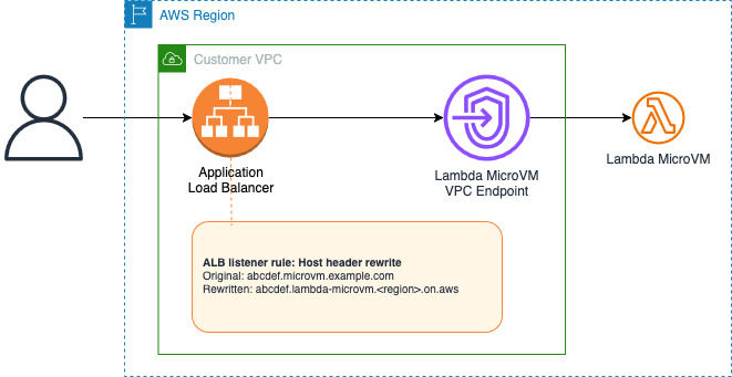
The request flow looks like this:

Request flow from a browser through the Application Load Balancer, which terminates TLS and rewrites the Host header, then forwards over AWS PrivateLink to the Lambda MicroVM service.

The key component is the ALB host header rewrite, introduced in URL and host header rewrite for Application Load Balancers. A listener rule matches the incoming custom host with a regex condition, captures the MicroVM ID from the left-most label, and a host-header-rewrite transform rewrites the Host header to <uuid>.lambda-microvm.<region>.on.aws before forwarding. Because the MicroVM service front-end routes on the Host header, the request lands on the correct MicroVM, while the customer’s domain stays in the browser’s address bar the whole time.

Why not CloudFront? Why not an ALB redirect?

  • CloudFront can also rewrite Host/SNI toward the origin, but a single distribution has static origins. Mapping a wildcard of MicroVM IDs through one distribution would require a CloudFront Function to compute the origin per request. The ALB transform performs the same rewrite for the entire wildcard with zero code.
  • An ALB redirect action only issues an HTTP 301 Moved Permanently/302 Found response. The browser would follow it, and the address bar would then show the .on.aws URL, which breaks our design as it is not a real custom domain. The transform (not a redirect) is what makes the custom domain transparent.

Walkthrough

The example is an AWS CDK application. Configuration lives under the microvm-custom-domains key in cdk.json (hosted zone, wildcard base, the endpoint base to rewrite to, the PrivateLink service name, and the CORS origin). Set those values, then deploy. The sections below explain what the stack creates and why.

Prerequisites

A small VPC (two Availability Zones, which is the minimum for an internet-facing ALB) hosts the ALB and an interface VPC endpoint to the AWS managed MicroVM service. There are no NAT gateways, because nothing here needs egress, which keeps the footprint lean.

// Interface (PrivateLink) endpoint to the AWS managed MicroVM service.
const endpoint = new ec2.InterfaceVpcEndpoint(this, 'MicroVmEndpoint', {
  vpc,
  service: new ec2.InterfaceVpcEndpointService(cfg.microvmVpceServiceName, 443),
  subnets: { subnetType: ec2.SubnetType.PRIVATE_ISOLATED },
});

2. Discover the endpoint’s private IP addresses at deploy time

An ALB IP target group needs the private ENI IP addresses of the interface endpoint (one per Availability Zone). CloudFormation does not expose those IPs as a usable attribute, so the stack resolves them during deployment with an AwsCustomResource that reads the endpoint’s own ENIs by ID (DescribeNetworkInterfaces on vpcEndpointNetworkInterfaceIds).

This is the only compute the package deploys, it runs only during cdk deploy, and it is never in the request path.

3. Request a wildcard TLS certificate

ACM issues a DNS-validated wildcard certificate for *.microvms.example.com, validated through the hosted zone you imported. The ALB presents this certificate for every custom domain under the wildcard.

4. Create the ALB and the MicroVM target group

The internet-facing ALB has an HTTPS:443 listener using the wildcard certificate. The target group holds the endpoint ENI IPs as IP targets, reached over HTTPS:443.

  • Encrypted in transit. A customer-provided AWS Certificate Manager (ACM) certificate is used to securely terminate encryption between the client and the ALB. The ALB re-originates TLS to the MicroVM service so traffic stays encrypted through the network.
  • IP-based targets. The target group uses IP-based targets with the local IP addresses of the VPC endpoints.
  • Health check matcher 200,403,404. The load balancer’s health probes are unauthenticated, so the MicroVM endpoint answers them with 403. A 403 here means “endpoint is reachable,” not “auth is broken,” so the matcher treats it as healthy.
const targetGroup = new elbv2.ApplicationTargetGroup(this, 'MicroVmTargets', {
  vpc,
  protocol: elbv2.ApplicationProtocol.HTTPS,
  port: 443,
  targetType: elbv2.TargetType.IP,
  targets: targetIps.map((ip) => new elbv2t.IpTarget(ip, 443)),
  healthCheck: {
    protocol: elbv2.Protocol.HTTPS,
    path: '/',
    healthyHttpCodes: '200,403,404',
  },
});

const listener = alb.addListener('Https', {
  port: 443,
  protocol: elbv2.ApplicationProtocol.HTTPS,
  certificates: [certificate],
  // Default action for anything that doesn't match our host regex.
  defaultAction: elbv2.ListenerAction.fixedResponse(404, {
    contentType: 'text/plain',
    messageBody: 'Unknown custom domain',
  }),
});

5. Add the host-header rewrite rule

A listener rule matches <uuid>.microvms.example.com with a regex condition and rewrites the Host header to <uuid>.lambda-microvm.<region>.on.aws with a host-header-rewrite transform. The regex captures the left-most label (the MicroVM ID) and reuses it in the replacement.

At the time of writing, the CDK L2 constructs don’t yet model regex host conditions or transforms, so the example reaches the underlying CfnListenerRule to set them:

const escapedBase = customDomainBase.replace(/[.]/g, '\\.');
const matchRegex = `^(.+)\\.${escapedBase}$`;     // capture <uuid>
const replaceWith = `$1.${microvmEndpointBase}`;   // <uuid>.lambda-microvm.<region>.on.aws

const cfnRule = forwardingRule.node.defaultChild as elbv2.CfnListenerRule;

cfnRule.conditions = [{ field: 'host-header', regexValues: [matchRegex] }];

cfnRule.addPropertyOverride('Transforms', [
  {
    Type: 'host-header-rewrite',
    HostHeaderRewriteConfig: { Rewrites: [{ Regex: matchRegex, Replace: replaceWith }] },
  },
]);

6. Point Route 53 at the ALB

Wildcard A and AAAA alias records (*.microvms.example.com) target the ALB, so every MicroVM custom subdomain resolves to it.

7. Deploy

Run the following commands to install the dependencies and then deploy the application.

npm install
npx cdk deploy

Handling CORS at the ALB

If your clients are browsers calling the MicroVM from another origin, CORS is handled entirely at the ALB, with no change to the application inside the MicroVM.

The listener uses ALB header-modification attributes to insert the Access-Control-Allow-* headers on every response. A higher-priority rule answers OPTIONS preflight requests at the edge with a fast 204 response. Otherwise, preflight requests would reach the origin and be rejected without an access token.

// Insert CORS headers on every response on this listener.
const cfnListener = listener.node.defaultChild as elbv2.CfnListener;
cfnListener.addPropertyOverride('ListenerAttributes', [
  { Key: 'routing.http.response.access_control_allow_origin.header_value',  Value: cfg.corsAllowOrigin },
  { Key: 'routing.http.response.access_control_allow_methods.header_value', Value: 'GET,POST,PUT,DELETE,OPTIONS,PATCH,HEAD' },
  { Key: 'routing.http.response.access_control_allow_headers.header_value', Value: 'x-aws-proxy-auth,x-aws-proxy-port,content-type,authorization' },
  { Key: 'routing.http.response.access_control_expose_headers.header_value', Value: 'content-type,content-length' },
  { Key: 'routing.http.response.access_control_max_age.header_value',        Value: '86400' },
]);

// Answer OPTIONS preflights at the ALB.
new elbv2.ApplicationListenerRule(this, 'CorsPreflightRule', {
  listener,
  priority: 10,
  conditions: [elbv2.ListenerCondition.httpRequestMethods(['OPTIONS'])],
  action: elbv2.ListenerAction.fixedResponse(204, { contentType: 'text/plain', messageBody: '' }),
});

Because the ALB adds those headers to both the preflight 204 and the forwarded MicroVM response, a browser’s cross-origin call succeeds without any application change. Set corsAllowOrigin to * for quick testing, and pin it to your own site for anything beyond a demo.

Test it end to end

First, launch a Lambda MicroVM and mint an access token (follow Create your first Lambda MicroVM). When it’s running, the service gives you a generated endpoint that looks like:

012345678-9abc-defg.lambda-microvm.us-east-2.on.aws

To get the custom-domain equivalent, replace the endpoint suffix (.lambda-microvm.<region>.on.aws) with your wildcard base: .microvms.example.com. Everything ahead of that suffix is preserved exactly:

012345678-9abc-defg.microvms.example.com

The ALB’s rewrite rule captures whatever precedes the suffix and re-attaches it to the real endpoint base, so the mapping holds for the entire wildcard. You never register anything per-MicroVM.

With your token in hand, call the custom domain you derived:

curl "https://012345678-9abc-defg.microvms.example.com/<path>" \
  -H "X-aws-proxy-auth: <token>" \
  -H "X-aws-proxy-port: 8080"

The request travels to the ALB, which terminates TLS, rewrites the host header, and forwards over PrivateLink to the MicroVM. The response comes back under your domain.

The reference architecture also includes a single-page demo and a POST /api/provision endpoint that runs or reuses a MicroVM and mints a short-lived token. With it, you can try the flow without wiring up token creation yourself. It even performs this suffix swap for you and hands back a ready-to-click custom-domain URL. See the repository for that piece.

Important considerations

  • Authentication is still the client’s job. This pattern only rewrites Host. The client must still supply a valid, unexpired access token in X-aws-proxy-auth. This is deliberate. MicroVM tokens are per-MicroVM and short-lived, so baking them into infrastructure would be fragile and insecure.
  • Region pinning. PrivateLink is regional, so the ALB, the endpoint, and the MicroVM service must all be in the same Region.
  • Production hardening. If you adapt the sample’s provisioning endpoint, put authentication and rate limiting in front of it, pin CORS to your origin, and scope IAM to the minimum. The sample’s provisioning path is intentionally open for demonstration and is not production-safe as written.
  • Cost. You pay for the ALB and the interface endpoint (hourly plus data processing) in addition to the Lambda MicroVM usage. There is no CloudFront distribution and no per-request compute in the data path.

Clean up

Run the following command in the same directory where you deployed the application from.

npx cdk destroy

This removes the ALB, target groups, endpoint, certificate, VPC, and Route 53 records created by the stack.

Conclusion

You can front AWS Lambda MicroVMs with customer-owned wildcard custom domains using an Application Load Balancer and AWS PrivateLink. The key is the ALB’s host-header rewrite. Because the MicroVM service routes requests based on the Host header, a single rewrite rule can transparently map an entire wildcard of custom domains onto your MicroVMs. CORS is handled at the edge as well. The whole setup relies only on networking primitives, with no CloudFront distribution and no compute in the request path.

To try it yourself, deploy the reference architecture and review the ALB URL and host header rewrite launch post for more on the transform feature.

Running self-hosted AI agent sandboxes with AWS Lambda MicroVMs

Post Syndicated from Brian Krygsman original https://aws.amazon.com/blogs/compute/running-self-hosted-ai-agent-sandboxes-with-aws-lambda-microvms/

Organizations are building AI agents that autonomously write code, query databases, and interact with internal systems on behalf of their teams. These agents handle use cases such as automated code review, data pipeline optimization, and infrastructure troubleshooting. When your AI agent generates a shell command, queries a database, or writes to a file system, that code needs a secure environment to run in. Without isolation, one session’s tool calls can contaminate another session’s state, inadvertently expose sensitive data across tenants, or unintentionally allow untrusted code to reach production resources. Self-hosted sandboxes solve this by keeping agent execution within your own AWS account, giving you full control over networking, secrets, and governance.

Say you’re building an internal AI agent that optimizes database queries for your engineering team. A developer asks it to find the ten slowest queries in your analytics database, rewrite them with better indexing, and test the results. That’s three tool calls in a single session. One hits a live database with real credentials. One generates code. One executes it. Now multiply that by fifty developers using the assistant at the same time. Each session needs its own credentials, its own filesystem, its own network boundary. If credentials or state cross session boundaries, you have inadvertent data exposure.

AWS Lambda MicroVMs is a serverless compute environment that provides general-purpose runtimes with the strong isolation of virtual machines and the rapid scaling of AWS Lambda. Powered by Firecracker virtualization, each MicroVM runs Amazon Linux with full OS access for up to 8 hours. You launch, suspend, resume, and terminate MicroVMs programmatically. You get the serverless benefits of managed infrastructure, responsive scaling, and pay-per-use pricing. Three capabilities make Lambda MicroVMs a strong fit for agent sandboxes:

  • VM-level isolation per environment: Each MicroVM runs in its own Firecracker virtual machine, providing hardware-virtualization-based isolation between sessions without the resource overhead and startup time required of full VMs. One developer cannot see a teammate’s session, even when both run at the same time.
  • Launch from snapshot: Like Lambda SnapStart, MicroVMs boot from a pre-captured memory and disk snapshot, skipping application initialization entirely. Your agent gets a near-instant ready-to-use environment.
  • 4x vertical scaling without re-provisioning: A running MicroVM can scale CPU and memory up to 4x its initial allocation, which can range from 0.25 vCPU/0.5 GB to 4 vCPU/8 GB, without terminating or re-creating the environment. If the agent needs to run a heavy data transformation mid-session, it can get more resources without starting over.

In this post, we show you how to architect and build a self-hosted AI agent that uses Lambda MicroVMs as secure, isolated sandboxes for tool-call execution. Lambda MicroVMs can handle the compute isolation for running tool calls, while the host for production AI agents, such as Amazon Bedrock AgentCore, manages the agent logic, model routing, and session state. A complete reference solution is available in aws-samples.

How self-hosted sandboxes work

A developer asks the agent to “find the ten slowest queries in our analytics database and suggest index improvements.” The agent orchestration system starts a session then breaks the objective into tool calls and distributes them. A worker needs to pick up that session, run the queries, and return results.

Most AI agent orchestration services and frameworks use a work queue model to distribute tool-call execution. The orchestration service enqueues sessions representing tool-call work. A worker, the process that claims a session and executes its tool calls, runs inside a compute environment, posts results, and exits. In this architecture, each Lambda MicroVM is the compute environment, and the worker is the process running inside it. Claude Managed Agents self-hosted sandboxes run those workers inside your own infrastructure rather than on a shared, multi-tenant compute pool. Your database credentials stay in your virtual private cloud (VPC). Your network, introspection, and governance rules apply.

You can trigger workers in two ways:

  • Webhook-triggered: The orchestration application sends a notification when a session is ready. Your control plane launches a worker on demand.
  • Always-on: A long-running process continuously polls the work queue for new sessions.

The Lambda MicroVMs lifecycle aligns with the webhook-triggered pattern, where each session produces one inbound event that launches a fresh MicroVM. Lambda MicroVMs support configurable idle policies. After a configurable idle period, a MicroVM suspends automatically, preserving disk and memory state. It resumes when inbound traffic arrives or when you call the resume API. The MicroVM runs for the duration of the session, the worker exits, and the idle policy suspends then finally terminates the VM. Lifecycle hooks allow you to run custom logic at key steps in the MicroVM lifecycle.

In contrast, the always-on pattern risks breaking the polling loop by suspending the MicroVM when idle, since there’s no inbound traffic between sessions. You could disable the configurable idle period, but then you pay for empty polling. Use the webhook-triggered approach for self-hosted sandboxes on Lambda MicroVMs.

Architecture

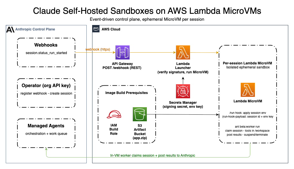
The following figure shows the reference solution’s architecture, with the Anthropic agent orchestration service control plane on the left interacting with a self-hosted sandbox environment in AWS on the right.

Reference architecture showing the Anthropic orchestration control plane sending a webhook through API Gateway to a launcher Lambda function that starts a MicroVM worker in your AWS account

Figure 1: Reference architecture for self-hosted AI agent sandboxes on Lambda MicroVMs

The sample architecture is event-driven. The only inbound traffic is the webhook call. When the event arrives, the handler launches a MicroVM. Once launched, the MicroVM pulls its assigned session from the orchestration system’s work queue and runs the task. In our example, the developer’s “find slow queries” request has been queued as a session. The agent now needs to reach your infrastructure, spin up an isolated environment, and hand off the work. The following sequence shows how each component interacts to fulfill a single session.

The orchestration service queues work as sessions. A MicroVM launches to service each session, and the worker is the process running inside that MicroVM that claims the session, executes tool calls, and returns results.

  1. Once the orchestration service marks a session as ready to run, it sends a session.status_run_started webhook to an Amazon API Gateway endpoint, triggering a MicroVM launch.
  2. The launcher verifies the webhook signature using a signing secret from AWS Systems Manager Parameter Store, rejecting invalid or stale deliveries before spending compute.
  3. The launcher calls RunMicrovm, passing the session ID and a secret reference through runHookPayload. It deduplicates on the webhook event ID (backed by Amazon DynamoDB) so retries do not launch duplicate VMs.
  4. The MicroVM boots from a pre-captured Firecracker snapshot and receives the dispatch on its /run lifecycle hook. The worker fetches the environment key from Parameter Store using its execution role. It pulls the matching session from the work queue, claims it, and executes tool calls in an isolated /workspace directory. When finished, it posts results and exits. The idle policy suspends then terminates the VM.

Deduplication. The webhook event ID serves as the idempotency key. The launcher uses Powertools for AWS Lambda (Python) with a DynamoDB persistence layer to verify exactly-once processing. If the orchestration application retries a delivery with the same event ID, Powertools protects the system from launching extra MicroVMs and doing extra work.

Credential boundaries. Each component accesses only the single secret it needs. The launcher reads only the webhook signing secret to verify inbound events. It passes only an ARN reference to the environment key into the MicroVM payload. The MicroVM’s execution role retrieves only that environment key at runtime. No single component holds both secrets.

Component Has access to
Launcher Lambda Webhook signing secret (verify inbound events)
MicroVM worker Environment key (through the execution role, to poll and claim sessions)

Cost model. You pay for MicroVM run time per session, plus standard charges for API Gateway requests, Parameter Store API calls, and Lambda invocations for the launcher. When no sessions are active, no MicroVMs run. Cost scales with concurrent sessions and their duration, avoiding idle compute charges.

Implementation

The following sections explore the reference architecture in more depth.

Project structure

The reference solution uses AWS Serverless Application Model (AWS SAM) for infrastructure-as-code. Alternatively, if you use an AI coding agent such as Claude Code, Kiro, or Cursor, the Agent Toolkit for AWS includes a Lambda MicroVMs skill that gives your agent the procedures to provision, configure, and deploy MicroVM-based sandbox environments on your behalf.

├── template.yaml                    # SAM: launcher, API, WAF, secrets, roles
├── src/
│   ├── functions/launcher.py        # Verify signature, RunMicrovm
│   ├── microvm-image/
│   │   ├── Dockerfile               # AL2023 + Node.js worker
│   │   └── worker/worker.mjs        # Lifecycle hook server
│   └── scripts/build-image.sh       # Package + create MicroVM image

Launcher: verify the webhook before spinning up compute

When the webhook arrives saying a developer’s session is ready, the launcher’s first action is signature verification. If it fails, the function returns 401 immediately. No MicroVM launches. No DynamoDB writes. You don’t pay for fraudulent or replayed requests.

signing_secret = [REDACTED_PASSWORD]  # Verify webhook before spending compute
if not verify_signature(raw_body, headers, signing_secret):
    return {"statusCode": 401, "body": "invalid signature"}

After verification, the launcher builds a dispatch payload containing the session ID, environment ID, region, and an ARN reference to the environment key secret. It passes this to RunMicrovm through runHookPayload:

launched = microvm_client.run_microvm(
    image_identifier="arn:aws:lambda:us-east-1:123456789012:microvm-image:worker",
    run_hook_payload=json.dumps({"session": dispatch}),
    execution_role_arn=config.execution_role_arn,
    maximum_duration_in_seconds=28800,
    ingress_network_connectors=["arn:aws:lambda:::network-connector:aws-network-connector:ALL_INGRESS"],
    egress_network_connectors=["arn:aws:lambda:::network-connector:aws-network-connector:INTERNET_EGRESS"],
)

MicroVM worker: claim one session, execute, exit

The MicroVM image is built from a Firecracker snapshot. The worker process starts during image creation and is captured in the snapshot, so there is no application startup at run time. The /run lifecycle hook delivers the dispatch payload:

// POST /aws/lambda-microvms/runtime/v1/run
case "run": {
    const envelope = JSON.parse(rawBody);
    const dispatch = JSON.parse(envelope.runHookPayload);
    res.writeHead(200); // Acknowledge hook immediately
    res.end();
    const key = await fetchParameter(dispatch.session.ENVIRONMENT_KEY_PARAM_NAME);
    await pollAndHandleSession(dispatch.session.ANTHROPIC_SESSION_ID, key);
    // Session complete; terminate this MicroVM to release all resources
    await terminateMicroVm(envelope.microvmId);
}

The worker acknowledges the hook within its timeout, fetches the environment key, and claims the session. This is where the requested work begins. The worker connects to the analytics database, runs EXPLAIN ANALYZE on the flagged queries, writes optimized alternatives to /workspace/suggestions.sql, and posts the results back to the developer. All of that happens inside this single VM. When the session completes, the worker calls terminate-microvm to release all compute resources.

Deployment

For full deployment instructions, see the reference solution README. Before deploying, make sure you have these prerequisites.

Prerequisites

Four steps

  1. Deploy the control plane. Build and deploy the SAM stack, which creates the launcher Lambda, API Gateway endpoint, WAF WebACL, DynamoDB idempotency table, Parameter Store entries, and MicroVM execution role.
    sam build
    sam deploy --guided --capabilities CAPABILITY_NAMED_IAM

  2. Register the webhook and populate secrets. In the Claude Console, register the stack’s WebhookUrl output as a webhook endpoint subscribed to session.status_run_started. Store the signing secret and environment key in the Parameter Store resources created by the stack.
  3. Build the MicroVM image. Package the Dockerfile and worker code, upload to Amazon S3, and create the image. The service runs your Dockerfile, launches the worker, and captures a Firecracker snapshot. Monitor build progress in Amazon CloudWatch under /aws/lambda/microvms/<image-name>.
    ./src/scripts/build-image.sh

  4. Verify. Create a test session and confirm a MicroVM launches and completes end-to-end. The reference solution includes a verification script that creates a session, triggers the webhook, and validates the full flow.

Using Claude Platform on AWS (CPOA)

The preceding architecture works similarly when you access Claude through Claude Platform on AWS rather than the first-party API. Three things change in the worker:

  1. Client initialization. Replace the first-party client with the AWS client and supply your workspace ID:
    from anthropic import AnthropicAWS
    
    client = AnthropicAWS(aws_region="us-east-1")
    
    # Workspace ID is required on every request
    # Set via ANTHROPIC_AWS_WORKSPACE_ID env var or pass per-call

  2. Authentication options. CPOA supports two modes:
    1. CPOA API key (aws-external-anthropic-api-key-...): Store it in Parameter Store the same way as the first-party environment key. These keys are short-lived (12-hour STS tokens) and must be regenerated when they expire.
    2. SigV4 (IAM): The MicroVM execution role can sign requests directly, so there is no secret to store or rotate. Set the environment key secret to a placeholder value (for example, use-sigv4) and the SDK falls through to IAM credentials automatically. This is the recommended path for production.

In both authentication modes, attach the AWS managed policy AnthropicSelfHostedEnvironmentAccess to the MicroVM execution role. This policy grants the aws-external-anthropic actions needed to poll the work queue, claim sessions, and post results. See IAM actions for Claude Platform on AWS for the full reference.

Prerequisite: Enable outbound web identity federation once per AWS account:

aws iam enable-outbound-web-identity-federation

Everything else, including webhook verification, deduplication, credential separation, and idle policy remains the same.

Security

Earlier we talked about what goes wrong without isolation. Credentials exposed between sessions. Scripts unintentionally reaching production. Agents escaping their sandbox. This architecture implements defense in depth to help prevent these.

Each component accesses a single, scoped secret. The launcher passes only an ARN reference to the worker credential into the MicroVM. The MicroVM’s execution role retrieves only that credential at runtime. The analytics database connection string does not touch the launcher and does not leave your environment.

AWS WAF applies managed rule sets (OWASP, known bad inputs, IP reputation) and per-IP rate limiting. Amazon API Gateway request validation rejects malformed bodies. The launcher performs HMAC signature verification as the true authentication boundary.

Each session runs in its own MicroVM. Sessions do not share memory, disk, or network namespaces. Firecracker provides hardware-virtualization-based isolation. The launcher IAM role reads only the signing secret. The MicroVM execution role reads only the worker credential. Both are scoped to specific Parameter Store ARNs. The Amazon S3 artifact bucket blocks public access, enables versioning, and uses server-side encryption.

Conclusion

This post walked through how to give your internal AI agent a safe place to run database queries, generate code, and execute scripts on behalf of fifty developers without leaking data between sessions or reaching resources it shouldn’t.

AWS Lambda MicroVMs provide ephemeral, VM-isolated compute environments that align with the per-session execution model of AI agent sandboxes. Snapshot-based launch avoids application startup latency. Idle policies terminate VMs once sessions complete. Firecracker isolation verifies that sessions do not share state. You pay only for active execution time and maintain full control over credentials, networking, and governance within your AWS boundary.

You build and operate a serverless control plane. You get per-session VM isolation with no idle compute cost and no shared tenancy.

To get started, explore these resources:

How CSIRO built scalable, cost-optimized genomic variant querying on AWS

Post Syndicated from Prof. Denis Bauer original https://aws.amazon.com/blogs/architecture/how-csiro-built-scalable-cost-optimized-genomic-variant-querying-on-aws/

This is a guest post by Denis Bauer, Yatish Jain, Anuradha Wickramarachchi, Brendan Hosking, and Nick Edwards of CSIRO, in collaboration with the ASP Prototyping and Scaling Team at AWS.

In this post, we describe how researchers at CSIRO, Australia’s national science agency, built Serverless Beacon (sBeacon), a scalable serverless solution for securely querying genomic variant data on AWS, underpinning production-scale clinical and research applications.

The Beacon protocol is the widely adopted standard for exchanging genomic and phenotypic data developed by the Global Alliance for Genomics and Health (GA4GH). It uses an API to define how data is shared, with the goal of enabling efficient and secure data discovery across international research and clinical networks.

sBeacon is a production-ready implementation of this standard, built using AWS services: Amazon Simple Storage Service (Amazon S3), AWS Lambda, Amazon DynamoDB, and Amazon Athena. By using these foundational AWS serverless services, sBeacon is able to provide the following benefits to researchers and clinicians needing to perform genomic variant querying:

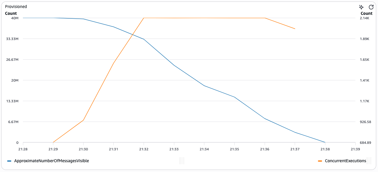
  • Highly scalable for large cohorts: sBeacon can scale to support hundreds of millions of individuals (and billions of genomic locations), which makes it suitable even for mega-biobank-scale datasets.
  • Low cost to run: Because it uses a serverless, cloud-native architecture, sBeacon can operate for approximately USD 0.40 per month for a 1000 Genomes-scale dataset. The following case study breaks down ingestion, query, and storage costs in detail.
  • High performance and fast query response: Real-world queries return in seconds (about 5 seconds) because of the serverless compute and efficient architecture, for near real-time data lookups.
  • No heavy data ingestion or transformation needed: sBeacon can directly consume standard VCF files (a common format for genomic variant data), which reduces the need to load data into databases or transform it to different data structures.
  • Rapid onboarding of new data: Genomic data generation is accelerating because it underpins clinical diagnosis and treatment, and because its complexity demands ever-larger cohorts to study complex traits. As a result, both clinical services and research cohorts must continuously onboard new data, and Beacon supports real-time generation-to-use life cycles (about 18 seconds).
  • Improved privacy, data ownership, and decentralization: Because sBeacon doesn’t require central databases and supports federated networks, data stays under the control of original holders, which can help data custodians address privacy and ethical considerations in sensitive genomic and medical data sharing.
  • Lower barrier to entry for broader participation: Its affordability, simplicity, and small operational footprint can help make it more accessible for smaller or resource-limited institutions and countries, which can increase participation from underrepresented populations and improve data diversity.
  • Zero trust model: sBeacon enforces explicit authentication, least-privilege data access, ephemeral compute isolation, and strict cloud-native boundary controls that help confirm no component, user, or request is implicitly trusted.

Prerequisites

sBeacon is deployed as a container that sets up the necessary development environment, with Terraform defining the resources for the deployment. To get started, clone the terraform-aws-serverless-beacon repository on the GitHub website.

git clone https://github.com/aehrc/terraform-aws-serverless-beacon.git

Make sure that your development environment contains Docker and has the necessary permissions for you to use it without super user access. Press Ctrl+Shift+P (Cmd+Shift+P on macOS) to open the command palette in VS Code, and then choose Reopen in Container. This opens the workspace in the container environment that we have defined.

Now, run the following command to initialize the necessary libraries and Lambda layers.

bash init.sh

Next, run the following command to initialize the Terraform environment.

terraform init

Optionally, you can define a backend by following the instructions in the repository. After the preceding command runs successfully, you can run the deployment command.

terraform apply

Enter yes when prompted to proceed with the deployment. After the deployment is complete, you receive information such as the API URL and the command to sign in as the admin or guest user. To shut down the entire service, run terraform destroy. Any created datasets are lost (but not the VCFs on which they are based).

Solution walkthrough

CSIRO developed sBeacon for sharing and querying genomic and medical data. sBeacon uses AWS serverless technology for the elastic scaling of compute resources.

The architecture of sBeacon performs two broad processes:

  1. Data onboarding: the ingestion and indexing of genomic metadata into sBeacon.
  2. Data querying: the querying of the genomic metadata by end users.

Data onboarding

During the onboarding process, you define where the genomic data and the metadata (such as disease status, age, and location) is located. Note that genomic data is not copied out of its original location but rather is referenced when needed. In contrast, metadata is loaded to sBeacon’s storage mechanisms because it is necessary to perform indexing that allows efficient querying. The user will need to ensure no sensitive or privacy-revealing data is disclosed. The example details the approach using CSIRO’s Ontoserver. However, sBeacon supports the API schema of the Ensembl OLS V4 specification.

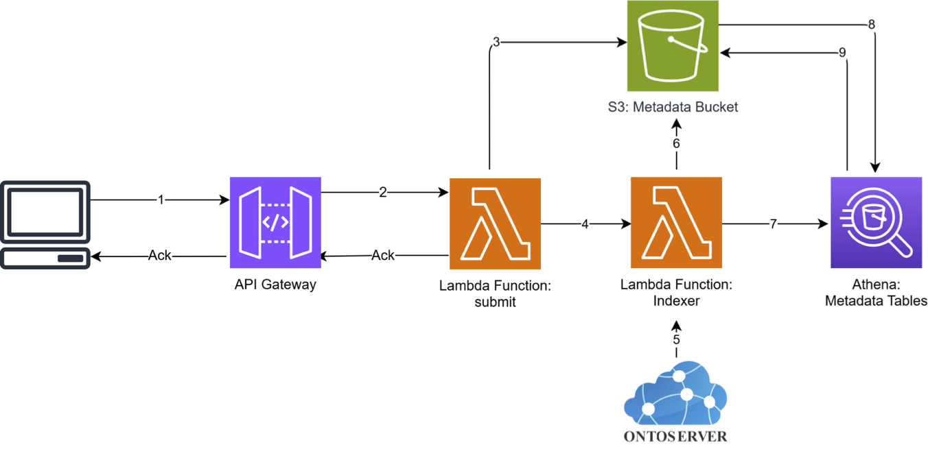
Data onboarding architecture for sBeacon, showing genomic data location submitted to an API Gateway endpoint, AWS Lambda functions handling indexing, metadata written to Amazon S3 in ORC format, CSIRO Ontoserver building the ontology index, and Amazon Athena building the metadata tables.

Figure 1. Data onboarding.

The data onboarding process is summarized by the following steps:

  1. The onboarding starts with the user submitting the location of the genomic data as request payloads to an API Gateway endpoint.
  2. The request payloads are forwarded to an AWS Lambda function that handles the data indexing.
  3. The metadata is written to an Amazon S3 bucket in the ORC format, to allow future querying and processing by Athena.
  4. An AWS Lambda function is called to orchestrate the indexing process.
  5. The CSIRO Ontoserver is called to build the ontology index for advanced metadata queries.
  6. The resulting index files are written to Amazon S3.
  7. CREATE TABLE AS SELECT (CTAS) queries are run on Amazon Athena to build the metadata tables.
  8. Athena loads the metadata from Amazon S3 into the metadata tables.
  9. The metadata tables are written back to Amazon S3 in ORC format.

Data querying

Querying in sBeacon is flexible, catering to a wide range of applications from human genetic disease to pathogen queries. We achieved this by designing the query architecture modularly. This approach let us separate the querying logic into several Lambda functions based on their querying scope, while maintaining a similar architecture.

The following architecture diagram describes the workflow for metadata querying, which uses the Variant Querying Module described later in this section.

Metadata querying architecture for sBeacon, showing a user query sent to an API Gateway endpoint, the Microservice Lambda function looking up ontology terms in Amazon DynamoDB, querying metadata tables in Amazon Athena, and querying the Variant Querying Module before returning a Beacon-formatted result.

Figure 2. Data querying.

  1. The user submits their query to the API Gateway endpoint.
  2. API Gateway calls the Microservice Lambda function.
  3. The Microservice Lambda function looks up the relevant query ontology terms in an Amazon DynamoDB table.
  4. The matching ontology descendent terms (and their codes) are returned to the Microservice Lambda function. The descendent terms are those that match a hierarchical descendent of each term, or each term itself, from the query.
  5. Using the ontology codes from step 3, the metadata tables on Athena are queried.
  6. The metadata associated with the query is returned from Athena.
  7. If required by the query, the Microservice Lambda function queries the Variant Querying Module.
  8. The variant data associated with the genomic conditions in the query is returned to the Microservice Lambda function.
  9. The result is formatted according to the Beacon protocol and is returned to the user through Amazon API Gateway.
  10. The response is received by the user.
Variant Querying Module architecture for sBeacon, showing an Initiator Lambda function fanning out the splitQuery and performQuery Lambda functions across VCF files in Amazon S3, and optionally querying metadata from Amazon Athena before returning results to the Microservice Lambda function.

Figure 3. Variant Querying Module.

Genomic variant queries are performed using the Variant Querying Module. The workflow of this module is as follows:

  1. The Microservice Lambda function calls an Initiator Lambda function.
  2. The Initiator Lambda function fans out the splitQuery Lambda function across the VCF files.
  3. The performQuery Lambda function is then fanned out across the VCF regions in each of the files involved in the query.
  4. The performQuery Lambda function fetches the VCF files from Amazon S3.
  5. The query results are synchronously returned to the parent Initiator Lambda function.
  6. If requested by the user, metadata can optionally be queried, where the Initiator Lambda function queries the metadata from Athena.
  7. Athena queries the metadata from Amazon S3 (through an external table).
  8. The metadata results are returned to Athena.
  9. The Initiator Lambda function receives the metadata from Athena.
  10. All the query results, including any optional metadata, are returned to the calling Microservice Lambda function.

Case study: 1000 Genomes dataset

We demonstrate sBeacon on chromosome 1 of the 1000 Genomes Project to report how it handles large-scale variant queries. We measure ingestion efficiency, query scalability, and cost for typical population-scale analyses, such as identifying SNP variants across defined genomic regions. The case study uses chromosome 1 (chr1, 8% of the genome) from the 1000 Genomes Project, which contains 2504 samples. This multi-sample VCF is approximately 1.1 GB compressed, with data stored in Amazon S3. Note that sBeacon can also process cohorts of single-sample VCF files. All costs in this section are for the Asia Pacific (Sydney) Region (ap-southeast-2), exclude applicable taxes, and reflect pricing at the time of writing.

sBeacon can ingest chromosome 1 from the 2504 individuals in 18 seconds, for less than 1 cent (USD 0.00052). This is because sBeacon does not copy the large genomic information but instead creates index files that enable random access. Cost is therefore driven predominantly by storing the copied metadata. After ingestion, sBeacon can be maintained for USD 0.000025 per month (1 MB of compressed metadata stored for 2504 samples in ORC format, plus genomic index files). If you store the genomic data as well, this would be USD 0.032 for chr1 (at USD 0.025 per GB in ap-southeast-2) or about USD 0.425 for the whole genome.

Query time is similarly near real time. For example, querying across a region of 10,000 base pairs to determine the genotypes in this region takes 1.52 seconds across the 2504 individuals. This would serve a query such as “Fetch all individuals with a specific BRCA1 mutation who have stage 3 cancer.” The cost for such a query is USD 0.00013. Note how the query time stays constant even with an increasing number of variants returned (for example, from 4 to 400).

Table 1. Query example costing and times (whole chromosome 1).

Query region size (bases) Number of variants found Average Time Compute Cost (per query in USD)
10 4 1.51 s (+- 0.26) 0.00013
100 18 1.52 s (+- 0.25) 0.00013
1,000 84 1.62 s (+- 0.24) 0.00014
5,000 229 1.65 s (+- 0.29) 0.00014
10,000 400 1.52 s (+- 0.11) 0.00013

Table 2. Cost for ingestion, querying, and idling (whole chromosome 1 for 2504 genomes with less than 10 MB of metadata).

Scenario Metric Cost (USD) per month
Ingestion Cost per 1000 ingestions 0.53 (32.82 GB seconds of Lambda)
Query compute cost per 1000 queries 0.28 (9.8 GB seconds of Lambda)
Query Athena Cost per 1000 queries 0.05
Idle Cost (Storage Cost) 1.1 GB 0.03
Query DynamoDB Cost Per 1000 queries 0.0005

Security features

Security and compliance is a shared responsibility between AWS and the customer. AWS is responsible for protecting the infrastructure that runs the AWS services described in this post, and you are responsible for your use of those services, including how you configure them, which identities you grant access to, and which data you choose to onboard. Consider the services you choose carefully, because your responsibilities vary depending on the services used, how you integrate those services into your IT environment, and applicable laws and regulations. For more information, see the AWS Shared Responsibility Model.

Zero trust model

  • Explicit authentication and authorization – Every API request must carry a valid JWT issued by the Amazon Cognito user pool (aws_api_gateway_authorizer.BeaconUserPool-authorizer, type COGNITO_USER_POOLS). The authorizer runs at API Gateway before any Lambda function is invoked, so requests do not reach a handler without Cognito validation. Token validation includes signature, expiry, and audience (Cognito app client ID). You can disable authentication during the first deployment with BEACON_ENABLE_AUTH = false for intentionally public or open beacons. This is an explicit operator decision, not a default.

Authorization (what a valid user can do) is enforced inside the Lambda layer, not in Amazon API Gateway:

  • Group membership (sbeacon-record-access-user-group, and so on) controls the maximum granularity returned.
  • Admin-only operations (dataset submission, deletion) check for sbeacon-admin-group membership before proceeding.
  • Least-privilege data access – sBeacon implements role-based access control (RBAC) through Cognito groups that map directly to disclosure tiers. You assign each user one or more of the following:
Cognito group Maximum disclosure
sbeacon-boolean-access-user-group exists: true/false only
sbeacon-count-access-user-group aggregate counts
sbeacon-record-access-user-group full variant details and sample names
sbeacon-admin-group preceding tiers plus dataset management

The JWT carries the user’s group memberships as claims. The query Lambda function reads these claims to determine requested_granularity and include_details, then passes both flags to performQuery. performQuery computes only what was requested. A boolean-tier user’s request does not cause sample-level data to be computed or returned, even if it exists in the VCF.

  • Ephemeral compute isolation – Lambda execution environments are stateless by design. Each cold start is a fresh container, /tmp (1,024 MB for performQuery) is cleared between cold starts, and concurrent invocations run in separate sandboxes with no shared memory. The bcftools subprocess inside performQuery runs and exits within the Lambda function lifetime (10 second timeout). No state persists after invocation.
  • Cloud-native boundary controls – API Gateway is the public entry point in this architecture. Amazon S3 buckets, DynamoDB tables, Athena, and Amazon SNS topics have no public resource policies. Amazon S3 buckets are created with private ACLs and BucketOwnerPreferred ownership controls. Lambda functions run on AWS-managed VPCs with no inbound network access. Amazon SNS topics are account-private (no external principal grants).

Privacy and data ownership

Each institution deploys the entire Terraform stack into its own AWS account, so there is no shared infrastructure, no central data lake, and no cross-account trust. VCF files live in the deploying institution’s Amazon S3 bucket and do not leave it. performQuery passes the Amazon S3 URL directly to bcftools as a subprocess argument, which uses htslib HTTP byte-range requests to read only the tabix-indexed region of interest (about 1 KB per query). The raw genomic sequence bytes do not pass through Lambda memory as returnable data. What the query returns upstream (exists as a boolean, call_count as an integer, and variant representations) is aggregate result data, not source sequence.

Decentralization in sBeacon is achieved at the storage layer, not the compute layer. The _vcfLocations registered for a dataset are Amazon S3 URIs, and these can point to buckets owned by entirely different organizations. When a query runs, performQuery passes each URI directly to bcftools, and htslib issues HTTP byte-range requests (Range: bytes=X-Y) against the Amazon S3 REST API of whichever organization owns that bucket. The raw VCF bytes do not leave the source organization’s Amazon S3 bucket. Only the query result (exists, count, or variant record) is returned.

Data onboarding privacy

The submitDataset endpoint sits behind the same API Gateway Cognito authorizer as all other endpoints. An unauthenticated request receives a 401 response before reaching any Lambda function. Beyond authentication, the handler also checks that the caller is a member of sbeacon-admin-group. A valid token from a user in only record-access or count-access is rejected. This means the beacon operator explicitly controls the set of people who can introduce data into the system, so onboarding is not a self-service capability.

Further considerations

We chose AWS Lambda over AWS Step Functions in this architecture because it can process much larger payloads. Given the size and complexity of genomic data and the fan-in and fan-out architecture for parallel handling, AWS Lambda emerged as the lower-cost and more flexible approach for this workload.

As demonstrated in the sBeacon publication, the architecture can cater to population-scale datasets. However, if you accidentally attempt to run a range query of the entire genome, the architecture times out at the Amazon API Gateway level. Applying functional operations over the whole genome requires further architectural considerations.

Because a single fan-out query spawns many parallel Lambda invocations, you need to monitor concurrency consumption to confirm that burst queries do not exhaust the account’s concurrency pool and starve other functions. Tracking the ConcurrentExecutions metric at both the account and function level provides early visibility into capacity pressure.

Similarly, because synchronous Lambda invoke does not automatically retry on throttle, a 429 response from a performQuery invocation means the result is silently lost unless the application handles it explicitly. Setting Amazon CloudWatch alarms on the Throttles metric for performQuery allows you to take corrective action, such as requesting a concurrency limit increase, before throttles affect query accuracy. Alternatively, we have produced a separate architecture that sends alert email with diagnostic information when Lambda functions fail, available in the error-catcher repository on the GitHub website. You can implement this in the repository or set it up as a standalone service to catch Lambda errors thrown by sBeacon.

After idle periods, simultaneous performQuery invocations might encounter cold starts that add latency to query responses. Enabling provisioned concurrency on the query-path Lambda functions helps reduce this cold-start latency during burst fan-out scenarios at the price of increasing the idle cost.

Conclusion

In this post, we described how CSIRO built sBeacon, a fast, scalable, and low-cost way to run genomics workloads on AWS. sBeacon implements the GA4GH Beacon standard with a fully serverless and modular architecture. This publicly available solution supports near real-time querying of standard VCF data, scales to mega-biobank cohorts, minimizes ingestion effort, and supports privacy and zero-trust security. If you are considering genomics on AWS, you can deploy sBeacon on existing Amazon S3-hosted VCF data, integrate it with clinical or research workflows through the Beacon API, and progressively federate with other Beacons for secure, cross-institutional genomic data discovery. Set up sBeacon to query your genomic data and explore the possibilities of securely sharing insights with your collaborators. You can read more about sBeacon in our publication: Scalable genomic data exchange and analytics with sBeacon. The source code for sBeacon can be downloaded from our GitHub repository.


About the authors

AWS Weekly Roundup: OpenAI GPT-6 Astra on Amazon Bedrock, Amazon Quick desktop GA, Kiro for students, and more (September 14, 2026)

Post Syndicated from Micah Walter original https://aws.amazon.com/blogs/aws/aws-weekly-roundup-openai-gpt-6-astra-on-amazon-bedrock-amazon-quick-desktop-ga-kiro-for-students-and-more-september-14-2026/

There’s a particular energy to mid-September in New York. Pumpkin spice lattes are flowing, temperatures are dropping, and it’s nearly sweater weather. The city is back at full speed, and so is the AWS launch calendar. This week that energy showed up in a new frontier model on Amazon Bedrock, a desktop app for Amazon Quick, and a reminder that the developers seeing the biggest gains from AI agents aren’t just using better tools — they’re working differently.

Let’s dive in.

Headlines
OpenAI GPT-6 Astra is now generally available on Amazon Bedrock – GPT-6 Astra is OpenAI’s latest and most capable model to date, and you can now run it on Amazon Bedrock. It brings deeper reasoning and judgment, professional-quality writing and design, and advanced computer and browser use to demanding business workflows. The model supports a context window of up to 1 million input tokens, so you can send it large codebases, long contracts, or extensive document collections and ask it to reconcile competing inputs.

You can call GPT-6 Astra through supported Amazon Bedrock APIs, or configure ChatGPT Work and Codex to use the model on Amazon Bedrock. Alongside the launch, OpenAI is introducing new enterprise plugins for ChatGPT Work that extend Astra’s browser-use capabilities across common business applications. Established AWS controls help you secure workloads, govern access, and audit model invocation activity, and your inference data isn’t used for model training. Read more

Last week’s launches
Here are some launches and updates from this past week that caught my attention:

  • Amazon Quick desktop app is now generally available on macOS and Windows – The Amazon Quick desktop app brings Amazon Quick to your computer, where it can work with local files and stay connected to your calendar, email, and business apps in the background. Conversations, context, and agents stay synchronized across desktop and mobile, so work you start on one surface carries over to the other. With this release, Quick agents also keep running after you close your computer, which means you can start a long-running task before you leave the office, add input from the mobile app on the way home, and review the result when you get there. Existing Quick users can download the desktop app, and the mobile app is available from the Apple App Store and Google Play. Read more
  • AWS Lambda now supports a 90-minute function timeout on Lambda Managed Instances – You can now configure a function timeout of up to 90 minutes for asynchronous and event source mapping (ESM) invocations on Lambda Managed Instances, a 6x increase from the previous 15-minute limit. That opens the door to data processing, media transcoding, financial calculations, AI inference, and batch jobs that need longer continuous execution, without splitting the work across multiple functions. Synchronous invocations keep the existing 15-minute maximum. The longer timeout also applies to steps inside Lambda durable functions, which can still run for up to a year when invoked asynchronously. Read more
  • Amazon EBS Volume Clones now copies volumes across accounts – Amazon Elastic Block Store (Amazon EBS) Volume Clones can now copy a volume into another AWS account and re-encrypt it with an AWS Key Management Service (AWS KMS) key in the target account. If you keep production and development in separate accounts, you can share a volume with AWS Resource Access Manager (AWS RAM) and let the target account create a fresh copy in the same Availability Zone, for example, cloning a production database volume into an isolated development account. Cross-account copy works for all volume types, including unencrypted volumes and volumes encrypted with customer managed keys. Read more
  • Second-generation single-rack AWS Outposts is now generally available – The new single-rack AWS Outposts is a self-contained 42U rack that puts compute, storage, and networking into one compact unit for locations that need low latency, local data processing, or data residency, and don’t have room for a larger footprint. A single rack delivers up to 2,688 vCPU and 100 TB of Amazon EBS storage, and supports the latest x86-powered Amazon EC2 instances, including general purpose (M7i, M8i), compute-optimized (C7i, C8i), memory-optimized (R7i, R8i), and Outposts accelerated networking instances. You get the same APIs, console, automation, governance, and security controls as multi-rack Outposts and AWS Regions. Read more
  • Amazon OpenSearch Serverless is now available on v0 by Vercel – You can now describe a search or AI application in natural language inside v0 by Vercel and get a full-stack app backed by Amazon OpenSearch Serverless. v0 provisions a collection, indexes your data, and uses the OpenSearch Serverless endpoint for full-text search and vector search for retrieval-augmented generation (RAG) workloads, without leaving the v0 interface. OpenSearch Serverless scales capacity up and down for you, so you can focus on the application instead of cluster management. You can provision under a new AWS account or link an existing one. Read more
  • AWS Transform for .NET modernization is now generally available via CLI – You can trigger an AWS-managed .NET modernization in AWS Transform custom with a single CLI command, then run it interactively or script it into an existing pipeline. The CLI sits alongside the existing AWS Transform for .NET experiences in the web application, Visual Studio IDE, Kiro Power, and MCP agents. Use it to upgrade language versions, migrate frameworks, optimize performance, and analyze codebases with transformations you can run as-is or customize. The .NET modernization transformation includes 50,000 free agent minutes per month. Read more

For a full list of AWS announcements, be sure to keep an eye on the What’s New with AWS page.

Other AWS news
Here are some additional posts and resources that you might find interesting:

  • Clare Liguori on frontier engineering – If you already use an AI coding assistant but don’t feel like you’re shipping much faster, start here. Clare Liguori, Senior Principal Engineer at AWS, published a practitioner’s manifesto on frontier engineering: ten principles, drawn from teams across Amazon, for changing how you build software with AI agents. The argument is direct. Software development has split in two, people who changed how they work with agents, and people who only changed their coding tools. Frontier engineering is not vibe coding. You spend the first weeks writing steering files, refactoring the codebase, and learning to decompose work for agents. Those weeks feel slower. The weeks after feel dramatically faster, because you’re no longer building the software directly — you’re building the agent setup that builds the software.
  • A free year of Kiro for students around the world – The Kiro Students program is expanding from 11 universities to 121 new schools across 16 countries. Eligible students get one year of Kiro with 1,000 credits per month and full access to paid features such as premium models and Kiro Web, no credit card and no trial timer. You can work in the IDE, the CLI, Kiro Web in a browser, or Kiro Crew. If you’re a student, sign up with your university email.
  • The state of AI for security: measuring what matters for trust – Security teams are using AI for triage, threat modeling, incident response, and code review, but a tool that flags everything doesn’t save time. In The state of AI for security, Anshumali Shrivastava and Neha Rungta introduce Deception Benchmark, a new evaluation that tests whether a model can tell a real vulnerability from code that looks risky but is actually safe. The benchmark includes 14,822 samples across 16 languages and more than 70 Common Weakness Enumeration (CWE) categories. Under standard prompting, precision landed in the mid-50s, about as likely to be inaccurate as accurate, and none of the 12 models tested kept both false positives and false negatives below 10 percent. The post links to the dataset, whitepaper, and submission workflow for verified scoring.
  • Build full-stack AWS applications in minutes with AI-powered scaffolding – Version 1.0 of the Nx Plugin for AWS is an open source toolkit of deterministic generators for APIs, websites, databases, and AI agents, plus the AWS infrastructure to run them. Each generator writes working, deployable code with security, observability, and type-safety already in place, so an AI assistant can assemble the foundation and spend its effort on your application logic. Bingo Industries used it to take a multi-agent operations chatbot from idea to production in less than 3 weeks. The plugin is open source on GitHub. Create a workspace with pnpm create @aws/nx-workspace and point your coding agent at the included MCP server.
  • The oldest architecture in computing – On All Things Distributed, Werner Vogels starts from a question customers always ask “Will AI take my job?”, and lands on memory. After spending time with Kiro Crew, he traces a line from Jeff Hawkins’ A Thousand Brains to how Crew stores, consolidates, and forgets across markdown files, a vector database, and a key-value index. His conclusion: the brain is the oldest architecture in computing, and the people who think hardest about how it works will build the next tools. Now, go build.

For a full list of AWS blog posts, be sure to keep an eye on the AWS Blogs page.

Upcoming AWS events
Check your calendar and sign up for upcoming AWS events:

Join the AWS Builder Center to connect with builders, share solutions, and access content that supports your development. Browse here for upcoming AWS-led in-person and virtual events and developer-focused events.

That’s all for this week. Check back next Monday for another Weekly Roundup!

— Micah

This post is part of our Weekly Roundup series. Check back each week for a quick roundup of interesting news and announcements from AWS!

Announcing 90-minute function timeout on AWS Lambda Managed Instances

Post Syndicated from Tarun Rai Madan original https://aws.amazon.com/blogs/compute/announcing-90-minute-function-timeout-on-aws-lambda-managed-instances/

AWS Lambda now supports a 90-minute function timeout for asynchronous and event source mapping (ESM) invocations on AWS Lambda Managed Instances (LMI), a capability of AWS Lambda. This is a 6x increase from the previous 15-minute limit. Customers running data processing, media transcoding, financial calculations, AI inference, and batch workloads can now use Lambda functions for jobs that require longer continuous execution, without re-architecting their applications. This also applies to invocations within Lambda durable functions, which use checkpoints to track progress and automatically recover from failures through replay, skipping completed work. When invoked asynchronously, a multi-step durable execution can run for up to 1 year.

Evolution of function timeout on Lambda

Lambda’s function timeout has increased over time, from 5 minutes at launch in 2014 to 15 minutes in 2018. As customers sought to use the simplicity of Lambda for data-intensive workloads, the 15-minute timeout limit forced architectural tradeoffs for applications where customers needed longer continuous execution time. Several patterns emerged:

  • Media processing: Speech-to-text transcription and video transcoding that routinely need longer than 15 minutes of continuous execution.

  • Financial calculations: Monte Carlo simulations, bond pricing, and portfolio risk analysis that are memory-intensive and often require longer than 15 minutes.

  • Data processing and ETL pipelines: Batch jobs processing multi-gigabyte datasets or aggregating data from external sources that exceed 15 minutes during peak volumes.

  • AI inference: Model testing and inference jobs (for example, reasoning tasks) that fit Lambda’s memory and CPU profile but exceed its timeout.

  • Web scraping and file transfer: Crawling external sites or pulling large file sets from vendors that exceed 15 minutes when sources respond slowly.

In each case, customers preferred Lambda’s simplicity but had to re-architect when jobs hit the 15-minute limit.

Fast forward to 2026, Lambda supports two form factors: functions (event-driven, 15-minute timeout), and MicroVMs for user or AI-generated just-in-time code (HTTP-driven, 8-hour duration). To allow customers to benefit from the simplicity of serverless compute with the flexibility and pricing model of EC2 for steady-state workloads, we extended the on-demand capacity mode of Lambda to add Lambda Managed Instances (LMI). With Lambda Managed Instances, you can process multiple concurrent requests per instance, access specialized compute configurations, and drive cost efficiency through EC2 pricing advantages, without managing infrastructure.

We also support Lambda durable functions (powered by the durable execution SDK) on both on-demand and LMI capacity modes. Durable functions provide application-level checkpointing and workflow-as-code: your code saves execution state using step() and wait() operations, and gracefully recovers from infrastructure failures by resuming from the last checkpoint rather than restarting from scratch. While a durable execution (the complete lifecycle of a durable function) can run for up to a year, each invocation was still limited to 15 minutes.

As customers onboard more workloads to serverless compute to benefit from its simplicity, they need longer continuous execution for data-intensive use cases like AI inference, media transcoding, scientific modeling, and financial calculations that do not fit Lambda’s 15-minute duration constraints. Today, we are extending the function timeout on Lambda Managed Instances to 90 minutes for asynchronous and ESM invocations. This includes invocations within a durable function, where a multi-step application can continue to run for up to 1 year when invoked asynchronously.

Activating 90-minute function timeout

You can now configure any Lambda function running on a Managed Instance with a timeout of up to 90 minutes (5,400 seconds) for async and ESM invocations. Synchronous invocations retain the existing 15-minute maximum. The function executes exactly as before: same runtime, same handler, same IAM execution role, same virtual private cloud (VPC) configuration. The only difference is that your function now supports longer continuous execution. Your initialization code (Init phase) is still limited to 15 minutes on Lambda Managed Instances.

To set the timeout, update your function configuration using the AWS CLI:

aws lambda update-function-configuration \
    --function-name my-data-processor \
    --timeout 5400 \
    --region us-east-1

Or in AWS CloudFormation / AWS Serverless Application Model (AWS SAM):

MyFunction:
  Type: AWS::Serverless::Function
  Properties:
    FunctionName: my-data-processor
    Runtime: python3.12
    Handler: app.handler
    Timeout: 5400
    MemorySize: 10240

You do not need to change any code. You can also update the timeout from the Lambda console under Configuration > General Configuration (Figure 1), or configure it through natural language prompts in your AI coding assistants (like Claude Code or Kiro) by installing the Agent Toolkit for AWS.

Lambda console General configuration page showing the function timeout field set to 90 minutes

Figure 1: Configuring Lambda function timeout

The change takes effect on subsequent invocations after the function timeout is updated. For event source mappings, allow a few minutes for the new configuration to propagate. Your existing observability setup continues to work as expected: Amazon CloudWatch metrics, AWS CloudTrail, and AWS X-Ray capture the full invocation lifecycle without any changes. For details, see monitoring Lambda functions and monitoring durable functions.

There is no additional charge for using the 90-minute timeout. Standard Lambda Managed Instances pricing applies.

90-minute timeout and durable functions

The 90-minute function timeout and durable functions are complementary. The function timeout (--timeout) controls how long each individual invocation can run, while the durable execution timeout (ExecutionTimeout in --durable-config) controls the total elapsed time from execution start to completion. Durable functions use checkpoints to track progress and automatically recover from failures through replay, re-executing from the beginning while skipping completed work. With today’s launch, each asynchronous invocation in a durable function running on a Managed Instance can now execute for up to 90 minutes continuously, while the corresponding durable execution can run for up to 1 year. For synchronous and event source mapping invocations, both the invocation and the corresponding durable execution are limited to 90 minutes.

For idempotent jobs (for example, an ETL pipeline step triggered by SQS), the extended timeout alone might be sufficient. If the host fails, the message returns to the queue and a fresh invocation starts. For jobs where re-execution is expensive (for example, a 40-minute inference run already 30 minutes in), combine both. Enable durable functions to checkpoint periodically, so a failure at minute 35 resumes from the last checkpoint rather than restarting from zero.

Invocation behavior: asynchronous, event source mappings, and synchronous

Asynchronous invocations (up to 90 minutes): If the function fails or times out, Lambda applies your configured retry policy (up to two retries by default) and routes failed events to your dead-letter queue or on-failure destination.

Event source mappings (up to 90 minutes): For SQS, configure your queue’s visibility timeout to be at least six times the function timeout. This gives Lambda enough time to retry if a function is throttled while processing a previous batch. Lambda validates this at event source mapping creation time, but does not prevent subsequent changes to queue or function settings that might create a mismatch.

For Amazon Kinesis and Amazon DynamoDB Streams, configure the maximum batching window and parallelization factor to account for longer processing times per batch.

If your batch contains multiple records and you want to avoid re-processing the entire batch when one record fails, enable partial batch failure reporting. This is available for SQS, Kinesis, DynamoDB Streams, Amazon Managed Streaming for Apache Kafka (Amazon MSK), and self-managed Apache Kafka event source mappings. With partial batch failures enabled, only the failed records are retried, not the entire batch.

Note that invocations for Amazon MQ ESM and Amazon DocumentDB (with MongoDB compatibility) ESM remain limited to 15 minutes.

Synchronous invocations (15 minutes maximum): Synchronous invocations retain the existing 15-minute maximum timeout. If you set your function timeout to greater than 15 minutes and invoke it synchronously, Lambda continues to apply the 15-minute timeout. The GetFunctionConfiguration API reports the configured timeout value.

To see which event sources invoke Lambda functions synchronously or asynchronously, refer to Lambda documentation.

Considerations and best practices

Because your functions now support longer continuous execution, consider these best practices for components that might be ephemeral in nature, such as network connections and credentials.

Networking: Make sure idle connection timeouts on downstream services (RDS, Amazon ElastiCache, external APIs) accommodate the full function duration. If your function routes traffic through a NAT Gateway, send keep-alive packets to prevent idle connections from being dropped (350-second idle timeout). Respect DNS TTL values for external hostname resolution. The AWS SDK handles this automatically, but custom HTTP clients might cache DNS records beyond their TTL.

Credentials: If your function acquires temporary credentials or tokens, verify they remain valid for the full execution duration or refresh them in the background.

Idempotency: Lambda does not guarantee exactly-once processing. With longer-running functions, the window for retries and duplicate deliveries increases. You can use Powertools for AWS Lambda to implement idempotency in your function code so that operations like payments or database writes produce the same result even if executed more than once. If you use Lambda durable functions, steps have at-least-once execution semantics by default. The SDK skips completed steps during replay, but steps that fail before checkpointing may re-execute. You can use execution names as idempotency keys for durable functions.

Conclusion

The 90-minute function timeout on Lambda Managed Instances addresses one of the most common customer needs for building data-intensive applications on AWS Lambda. Data processing, media transcoding, AI inference, and financial computation workloads that exceed 15 minutes can now run on Lambda without code changes or architectural workarounds. We look forward to hearing from you if you need a longer timeout for synchronous invocations, or for the on-demand capacity mode, on our AWS Lambda Roadmap GitHub page.

To get started, update your function’s timeout configuration and deploy. For a step-by-step walkthrough, see Getting started with Lambda Managed Instances. For sample code demonstrating long-running functions with durable checkpointing, see durable functions examples. To learn more about AWS Lambda, visit aws.amazon.com/lambda.

AWS Weekly Roundup: Claude Fable 5.1 on AWS, Amazon Linux 2027 preview, AWS Certified AI Business Strategist, and more (September 7, 2026)

Post Syndicated from Channy Yun (윤석찬) original https://aws.amazon.com/blogs/aws/aws-weekly-roundup-claude-fable-5-1-on-aws-amazon-linux-2027-preview-aws-certified-ai-business-strategist-and-more-september-7-2026/

Last week, Claude Fable 5.1 became available on AWS. According to Anthropic, Claude Fable 5.1 delivers frontier intelligence for ambitious tasks across coding, scientific research, and enterprise workflows. Claude Fable 5.1 is built for long-running, high-stakes work that runs for hours and spans many applications. It can own more of a software project on its own, handling features across an entire codebase, code review, and performance work over extended sessions.

Anthropic has designated Fable 5.1 a Covered Model, a category of Claude models that carry additional data retention, safety review, and access policies wherever they’re offered. Claude Fable 5.1 is subject to data retention for up to 30 days and human review by Amazon personnel, with a new aws_review data retention mode. In this mode, AWS retains your prompts and outputs for human safety review within the AWS boundary. The provider_data_share mode is legacy, and Amazon Bedrock does not share your data with the model provider. In addition, Enterprise Frontier Safeguards (EFS), built in partnership between AWS and Anthropic, will let eligible customers use Covered Models while keeping their data in a cloud environment they control.

You have two ways to access Claude Fable 5.1: Amazon Bedrock and Claude Platform on AWS. To learn more, see the Claude Fable 5.1 model card on Amazon Bedrock and Claude Platform on AWS.

Last week’s launches
Here are some launches that got my attention:

  • Amazon Linux 2027 (AL2027) in public preview: AL2027 is the next version of the Amazon Linux operating system. It runs on kernel 7.1+, purpose-built for cloud-native workloads on AWS with performance, scale, and security in mind. Built on AL2023’s baseline, AL2027 is designed for customers who need a secure, stable, and AWS-native operating system running web applications, databases, containerized microservices, AI/ML workloads, and large-scale infrastructure.
  • Amazon EC2 R9g and R9gd memory-optimized instances: These instances are powered by AWS Graviton5 processors, delivering the best price performance for memory-intensive workloads running on Amazon EC2. R9g and R9gd instances deliver up to 25% better compute performance compared to AWS Graviton4-based R8g and R8gd instances. They are up to 30% faster for databases, up to 35% faster for web applications, and up to 35% faster for machine learning. To learn more, read Daniel’s blog post.
  • AWS Lambda SnapStart for container image functions: Lambda SnapStart is an opt-in capability that makes it easier for you to build highly responsive and scalable applications without provisioning resources or implementing complex performance optimizations. Previously, SnapStart was only supported for managed runtimes (Python, .NET, and Java). You can now use SnapStart for container images to reduce startup times from several seconds to as low as sub-second for latency-sensitive workloads such as ML inference and interactive APIs.
  • AWS Agent Registry now generally available: AWS Agent Registry provides a private, governed catalog and discovery layer for agents, tools, skills, MCP servers, and custom resources within your organization. In addition to the capabilities launched in preview (manual and URL-based record creation, approval workflows, semantic and keyword search, and AWS CloudTrail audit trails), Registry now adds new enterprise features. To learn more, visit the AI Blog post.
  • Amazon Redshift now supports Apache Iceberg v3 tables: You can read from and write to Apache Iceberg v3 tables in your data lake of Amazon Redshift. With this launch, Amazon Redshift introduces support for default column values, row lineage, and deletion vectors. Amazon Redshift’s Graviton based provisioned and serverless clusters support the new v3 format. To learn more, visit Apache Iceberg v3 features in Redshift.

For a full list of AWS announcements, be sure to keep an eye on the What’s New with AWS page.

Other AWS news
Here are some additional projects and news items you may find interesting:

  • AWS named a Leader in the 2026 Gartner Magic Quadrant for Strategic Cloud Platform Services: For the 16th consecutive year, Gartner has recognized AWS as a Leader in the 2026 Gartner Magic Quadrant for Strategic Cloud Platform Services, and once again placed AWS highest on the Ability to Execute axis. We believe this recognition reflects our commitment to delivering the broadest and deepest set of cloud capabilities from infrastructure and AI to security and operations, so you can build, innovate, and scale with confidence.
  • AWS Certified AI Business Strategist: This new certification targets professionals who evaluate, champion, and scale AI initiatives in their organizations: line-of-business leaders driving adoption across their teams, sales professionals articulating AI value to customers, consultants guiding client strategy from experimentation through production, program managers aligning AI investments to business outcomes. Beta exam registration opened September 1, 2026, with exam delivery beginning September 29.
  • Agentic Security: Detection and Response at Machine Speed: We believe security should evolve ahead of AI adoption, not behind it. That belief drove our team to collaborate with the SANS Institute on a new chapter in the 2026 Cloud Security Exchange eBook, where we lay out a practical framework for securing agentic workloads at enterprise scale. Our chapter goes deeper on securing agentic workloads, with specific architectural patterns, implementation guidance, and frameworks for security teams at every stage of agentic AI maturity, whether you’re evaluating, piloting, or operating at scale.

For a full list of AWS blog posts, be sure to keep an eye on the AWS Blogs page.

Learn more about AWS, browse and join upcoming AWS-led in-person and virtual events, startup events, and developer-focused events including AWS re:Invent, AWS Summits, and AWS Community Days. Join the AWS Builder Center to connect with builders, share solutions, and access content that supports your development.

That is all for this week. Check back next Monday for another Weekly Roundup!

— Channy

AWS Weekly Roundup: Welcome DuckLabs to the team, Agentic Resource Discovery (ARD), and more (August 31, 2026)

Post Syndicated from Daniel Abib original https://aws.amazon.com/blogs/aws/aws-weekly-roundup-welcome-ducklabs-to-the-team-agentic-resource-discovery-ard-and-more-august-31-2026/

The news that interested me the most last week was the DuckLabs acquisition. AWS has signed a definitive agreement to acquire DuckLabs, the Amsterdam-based company behind DuckDB, the popular open source analytical database that runs in-process and executes SQL directly against files like Parquet, CSV, and JSON. DuckDB stays open source under its independent foundation and the MIT license, and over time AWS plans to combine its speed at everyday queries with the enterprise scale of services like Amazon S3, Amazon Redshift, and Amazon Athena.

Co-founded by Hannes Mühleisen and Mark Raasveldt, DuckDB runs locally or on Amazon S3, which makes it remarkably fast for the everyday queries (a terabyte or less) that make up the bulk of real-world analytics. It also happens to pair beautifully with AI agents, which “poke” and experiment their way through data much like humans do. The co-founders will continue leading its technical direction while AWS combines DuckDB’s speed with analytics services like Amazon EMR, AWS Glue, and Amazon SageMaker. For the bigger picture on why this matters, Andy Warfield, Vice President and Distinguished Engineer shared his thoughts on the post DuckDB and the changing physics of analytics on All Things Distributed.

Now, let’s get into this week’s AWS news…

Last week’s launches
Here are some launches and updates from this past week that caught my attention:

  • Amazon ECS now automatically detects and recovers container instances that lose agent connectivity – Amazon ECS now continuously monitors agent connectivity to the control plane and surfaces a new AGENT_CONNECTIVITY health event across AWS Fargate, Amazon ECS Managed Instances, and Amazon ECS on EC2. On Fargate and Managed Instances, ECS handles recovery automatically, draining tasks, launching replacements, and deregistering the impaired instance. On EC2, you can wire the event into your own workflow. Available at no additional cost in all AWS Commercial and AWS GovCloud (US) Regions.
  • AWS Lambda introduces public preview runtimes, starting with Node.js 26 and Python 3.15 – You can now test upcoming Lambda runtimes before they reach general availability. Preview runtimes use the same identifier as the eventual GA version, so your functions graduate automatically with no action required. Third-party tools and deployment frameworks can also validate compatibility ahead of GA. Not meant for production yet (breaking changes are possible), but a great way to get ahead of your next upgrade. Available in all AWS commercial, AWS GovCloud (US), and China Regions.
  • AWS IoT Core adds a native InfluxDB rule action – You can now route time-series data from your IoT devices straight into InfluxDB (Amazon Timestream-managed or self-hosted) without writing custom code or standing up an intermediate service. IoT Core formats data into InfluxDB’s line protocol and supports device-side and server-side batching. Available in all AWS Regions where Amazon Timestream for InfluxDB is offered.
  • Amazon GameLift Servers now includes enhanced DDoS protection – Your game servers now get automatic protection against network and transport layer (layers 3 and 4) DDoS attacks – UDP reflection, SYN floods, and similar vectors – with nothing to enable or opt into. Built on top of AWS Shield Standard with gaming-optimized traffic shaping, it turns on the moment your servers start running (Server SDK 5) at no extra cost. It’s available in all supported GameLift Servers Regions except China (Beijing) and China (Ningxia).
  • Amazon SageMaker HyperPod expands support for Ray – You can now run Ray workloads on SageMaker HyperPod with built-in observability, resilient training, and accelerated inference. Create and manage Ray clusters from Amazon SageMaker Studio, attach JupyterLab or your local IDE so a multi-node cluster behaves like a local dev environment, and get auto-provisioned Grafana dashboards. Node auto recovery, hung job detection, and tiered checkpointing keep large training runs healthy, while Ray Serve adds a tiered KV cache for inference. Your existing open source Ray code runs unchanged. Available for HyperPod clusters orchestrated by Amazon EKS.

For a full list of AWS announcements, be sure to keep an eye on the What’s New with AWS page.

Other AWS news
Here are some additional posts and resources that you might find interesting:

  • Happy 20th birthday, Amazon EC2! – Amazon EC2 turns 20. Channy Yun looks back at how EC2 grew from a single m1.small instance type in one Region to more than 1,200 instance types across 39 Regions, along with the custom silicon journey from the first Graviton to Graviton5 and Trainium3. A fun and worthwhile read on the service that still underpins so much of AWS – including Amazon ECS, Amazon EKS, AWS Lambda, Amazon SageMaker, and Amazon Bedrock.
  • Agentic Resource Discovery (ARD): an open specification for agent discovery – As organizations scale up agents, tools, and MCP servers, those resources end up scattered across clouds, on-premises infrastructure, and SaaS platforms – each with its own registry and metadata. ARD is a new open specification (Apache 2.0) that defines a common way to describe and discover agentic resources, so publishers “describe once” and consumers “discover everywhere” – think DNS, but for agents. AWS contributed feedback but doesn’t own the spec, and it complements the AWS Agent Registry by letting you federate across catalogs without migrating.
  • Get started with the Agent Toolkit for AWS in the AWS CLI – A single AWS CLI command (aws configure agent-toolkit) now equips AI coding agents like Kiro, Claude Code, Codex, and Cursor with curated, up-to-date AWS knowledge and a secure connection to thousands of AWS APIs through the AWS MCP Server. If you build with an AI coding assistant, this helps it choose the right services, use modern APIs, and follow security best practices – so it gets AWS code right more often the first time.

Upcoming AWS events
Check your calendar and sign up for upcoming AWS events:

  • AWS Summits – Free in-person events where builders come together to learn, connect, and explore the latest in cloud and AI. Upcoming stops include Zurich (September 2), São Paulo (September 3), Tel Aviv (September 10), and Dubai (September 30). Can’t attend in person? You can stream sessions through the Global Livestream and On-Demand Hub. I’ll be presenting two sessions on generative AI and Amazon Bedrock at the São Paulo Summit – if you’re there, come say hello.
  • AWS Community Days – Community-led conferences where content is planned, sourced, and delivered by community leaders. Upcoming events include JAWS SONIC 2026 in Tokyo (September 5) and Warsaw, Poland (September 8).

Join the AWS Builder Center to connect with builders, share solutions, and access content that supports your development. Browse here for upcoming AWS-led in-person and virtual events and developer-focused events.

That’s all for this week. Check back next Monday for another Weekly Roundup!

— Daniel Abib

This post is part of our Weekly Roundup series. Check back each week for a quick roundup of interesting news and announcements from AWS!

Implement custom authentication for tools integration using request Lambda interceptor in AgentCore Gateway

Post Syndicated from Nishant Mainro original https://aws.amazon.com/blogs/security/implement-custom-authentication-for-tools-integration-using-request-lambda-interceptor-in-agentcore-gateway/

When deploying AI agents with Amazon Bedrock AgentCore, organizations benefit from built-in modern support for OAuth 2.0, AWS Identity and Access Management (IAM), and API key authentication through Amazon Bedrock AgentCore Gateway. However, some enterprise environments still use legacy authentication mechanisms such as HTTP Basic Authentication (Basic Auth) (RFC 7617). The extensible architecture of AgentCore Gateway enables support for these authentication mechanisms through a request Lambda interceptor—custom code that runs each time an agent calls a tool.

In this post, we show you how to use a request Lambda interceptor to authenticate to a downstream tool API using system credentials, retrieving a service account credential from AWS Secrets Manager and constructing a Basic Auth header. This design keeps credentials isolated from the agent, designed to mitigate exposure through model-driven behavior such as prompt injection.

Important: Basic Auth is an antiquated technology that transmits credentials as Base64-encoded text and should not be used as a long-term authentication strategy. AWS recommends modernizing to OAuth 2.0, SAML, OpenID Connect, or IAM where possible. However, some organizations with legacy workloads choose to decouple authentication modernization from their agentic AI adoption, addressing each on independent timelines. If your environment requires Basic Auth integration as an interim measure, consult your AWS Solutions Architect to evaluate the security trade-offs before proceeding. We’re providing this post as a reusable implementation, but it shouldn’t be construed as an endorsement of Basic Auth, or considered suitable as a long-term solution.

Solution overview

The solution uses a request Lambda interceptor in AgentCore Gateway to retrieve system credentials and construct a Basic Auth header for the downstream tool API. Figure 1 shows the end-to-end flow.

Figure 1: Solution workflow

Figure 1: Solution workflow

  1. The AI agent initiates a tool call over Model Context Protocol (MCP) to the gateway with an inbound JSON Web Token (JWT) issued by a configured identity provider (IdP). The MCP request body contains the tool name and any required parameters. The gateway’s inbound authentication layer validates the token against the IdP specified in the inbound authorizer configuration.
  2. After inbound authentication succeeds, the gateway invokes the request Lambda interceptor, passing the original request payload and headers, including the validated JWT and its embedded claims.
  3. The request Lambda interceptor re-validates the inbound JWT issued by the configured IdP as a defense-in-depth measure, then retrieves the system service account credential from Secrets Manager. The credential is a service account that authenticates the AI agent to the downstream tool.
  4. The interceptor then constructs a compliant Basic Auth header using the system credential and adds it to the outbound request. Because Basic Auth transmits credentials as Base64-encoded text (not encrypted), you must implement relevant compensating controls (e.g., ensure that all communication with the downstream tool API is over TLS, conduct two-person review of Lambda code changes, and so on).

    Note: The system credential stored in Secrets Manager corresponds to a service account in Active Directory (AD). The credential lifecycle requires a one-time manual seed: a system administrator creates the service account in AD and stores the same initial credential in Secrets Manager (necessary because Secrets Manager can’t read a password back from AD). As a security best practice, trigger an immediate rotation after seeding to retire the human-known password using the built-in capabilities of Secrets Manager. From that point forward, Secrets Manager automates the rotation process, periodically generates a new password, and updates both Secrets Manager and AD simultaneously. This eliminates manual credential management in either system. At runtime, the request Lambda interceptor retrieves the current credential from Secrets Manager and presents it to the downstream tool, which validates it against AD. For implementation details on keeping both stores synchronized, see Rotate Active Directory credentials stored in AWS Secrets Manager.

  5. The AgentCore gateway forwards the adjusted request now carrying the custom authentication header to the downstream target tool.
  6. The downstream target tool authenticates the request, processes it, and returns the response to the gateway.
  7. The gateway relays the response back to the AI agent.

Implementation

The following steps walk through configuring the request Lambda interceptor and implementing the core of the authentication transformation logic. You can find the complete sample code at Implementing custom authentication for tools integration using Request Lambda Interceptor.

Step 1: Attach a request Lambda interceptor to your AgentCore Gateway

Configure the AgentCore gateway to invoke a request Lambda interceptor for authentication transformation before forwarding the request to the downstream tool.

Important: You must enable passRequestHeaders configuration. Without it, the request Lambda interceptor can’t receive the request header containing the inbound JWT, and the authentication pattern described in this post will not work.

The following example shows the gateway configuration:

import boto3 

bedrock_client = boto3.client('bedrock-agentcore-control', region_name='<your-region>') 
# e.g., region_name='us-west-2' 

bedrock_client.update_gateway( 
    gatewayIdentifier='<your-gateway-id>', 
    interceptorConfigurations=[
        { 
            'interceptor': { 
                'lambda': { 
                    'arn': 'arn:aws:lambda:<region>:<account-id>:function:<YourInterceptorFunction>' 
                } 
            }, 
            'interceptionPoints': ['REQUEST'], 
            'inputConfiguration': { 
                'passRequestHeaders': True 
            } 
        } 
    ] 
) 

Step 2: Validate the inbound JWT

The interceptor independently validates the JWT signature as a defense-in-depth measure, protecting against scenarios where the request Lambda interceptor could be invoked through a path that bypasses gateway validation. It fetches the identity provider’s JSON Web Key Set (JWKS) (cached across warm Lambda invocations to avoid repeated network calls), verifies the token’s signature, expiration, and issuer, then returns the decoded claims.

The following code demonstrates JWT validation:

  import jwt 
  from jwt import PyJWKClient 

  COGNITO_ISSUER = 
  f"https://cognito-idp.{COGNITO_REGION}.amazonaws.com/{YOUR_COGNITO_USER_POOL_I 
  D}" 
  jwk_client = PyJWKClient(f"{COGNITO_ISSUER}/.well-known/jwks.json") 

  def validate_jwt(token): 
      """Validate JWT signature and return decoded claims.""" 
      signing_key = jwk_client.get_signing_key_from_jwt(token) 
      return jwt.decode(token, signing_key.key, algorithms=["RS256"], 
  issuer=COGNITO_ISSUER) 

Step 3: Retrieve system credentials from Secrets Manager

The interceptor retrieves the system service account credential from Secrets Manager. This credential authenticates the AI agent to the downstream tool. The secret is encrypted with a customer-managed AWS Key Management Service (AWS KMS) key and cached in memory for the configured time-to-live (TTL) to minimize API calls while ensuring rotated credentials are picked up promptly.

The following code retrieves the credential from Secrets Manager:

  import boto3 
  secrets_client = boto3.client('secretsmanager') 

  def get_system_credentials(): 
      """Retrieve the system service account credential from Secrets Manager.""" 
      response = secrets_client.get_secret_value( 
          SecretId=os.environ['SYSTEM_CREDS_SECRET_NAME'] 
      ) 
      return json.loads(response['SecretString']) 

IAM permissions: The interceptor’s execution role requires secretsmanager:GetSecretValue scoped to the specific secret Amazon Resource Name (ARN), and kms:Decrypt scoped to the KMS key used to encrypt it. Follow the principle of least privilege by restricting the resource ARN rather than using wildcards.

Note: The agent doesn’t have access to Secrets Manager. Only the request Lambda interceptor—a deterministic function not influenced by model behavior—retrieves credentials. This isolation is designed to mitigate the risk of adversarial prompts instructing the model to access or exfiltrate authentication credentials, even if the agent is compromised.

Step 4: Construct the Basic Auth header

The request Lambda interceptor constructs the Basic Auth header using the system credential retrieved for the downstream tool.

The following code shows the core transformation logic.

  def build_system_auth_header(headers): 
      """Validate JWT and construct Basic Auth header with system credential.""" 
      auth_header = headers.get('Authorization', '') 
      if not auth_header.startswith('Bearer '): 
          return _error_response(401, "No Bearer token found in request.") 

      # Validate JWT (defense-in-depth) 
      claims = validate_jwt(auth_header[7:]) 
      if not claims: 
          return _error_response(401, "JWT validation failed.")
          
      # Retrieve system credential from Secrets Manager 
      creds = get_system_credentials()
      
      # Construct Basic Auth header (RFC 7617) 
      basic_auth_encoded = base64.b64encode( 
          f"{creds['username']}:{creds['password']}".encode() 

      ).decode() 
      headers['Authorization'] = f"Basic {basic_auth_encoded}" 
      return headers 

Conclusion

A request Lambda interceptor in Amazon Bedrock AgentCore Gateway can bridge the gap between the authentication patterns supported by the gateway and the authentication requirements of legacy tool APIs that haven’t yet migrated to modern authentication standards. As demonstrated in this post, the interceptor validates the inbound JWT, retrieves system credentials from Secrets Manager, and constructs the downstream tool’s Basic Auth header without modifying tool schemas or agent implementation.

This approach is an interim integration pattern, not a target architecture. It introduces a credential that must be synchronized between Secrets Manager and the tool’s identity store (such as Active Directory), adding operational overhead for rotation, drift detection, and lifecycle management. The recommended path is to modernize the downstream tool to accept OAuth 2.0, SAML, or OpenID Connect, eliminating stored credentials entirely. Until that modernization is complete, the interceptor isolates credential handling from the agent runtime, designed to help ensure that the agent—a non-deterministic system influenced by user prompts—does not have access to authentication secrets.

If you have feedback about this post, submit comments in the Comments section below.


Nashant Mainro

Nishant Mainro

Nishant is a Senior Security Solutions Architect with Amazon Web Services, based in Atlanta, Georgia. He brings 17+ years of security experience, focusing on securing AI and agentic workloads. He enjoys architecting security controls at scale, including identity, authorization, and data access for AI agents, empowering customers to confidently build generative AI applications and protect their data on AWS.

Author

Ram Ramani

Ram is a technology leader in AI security focusing on AI-driven software development, AI for security, and building secure agents. Ram advises leaders, developers and architects on how to make an organization AI-native and secure while benefiting from velocity provided by AI-driven development.

Streamline your GitHub journey with AWS CodePipeline and AWS DevOps Agent

Post Syndicated from Anjani Reddy original https://aws.amazon.com/blogs/devops/streamline-your-github-journey-with-aws-codepipeline-and-aws-devops-agent/

Introduction

When CI/CD deployment failures occur for GitHub hosted applications,  AWS DevOps Agent reduces the hours that Development and Site Reliability Engineering (SRE) teams typically spend manually investigating across multiple AWS services, logs, and pipeline stages. This process delays critical deployments and impacts software delivery velocity. This is especially true when teams need to correlate data between GitHub commit histories, AWS CodePipeline execution logs, and Amazon CloudWatch metrics. When continuous integration and continuous delivery (CI/CD) pipelines fail, engineers often find themselves context-switching between GitHub pull requests, code build logs, deployment artifacts, and downstream service health metrics. This process of identifying root causes can extend resolution time from minutes to hours, especially in multi-service architectures.

AWS DevOps Agent reduces this manual investigation by automatically correlating pipeline failures with specific code changes. Rather than spending hours manually tracing deployment failures through multiple systems, engineers can use AWS DevOps Agent to perform this correlation. It identifies which specific code changes caused pipeline failures and provides remediation guidance. The agent analyzes pipeline failures, correlates them with specific commits and pull requests, and identifies root causes across the deployment chain.

AWS CodePipeline combined with AWS DevOps Agent helps address this challenge by creating a streamlined path from GitHub repositories to AWS deployments. This solution reduces manual handoffs, reduces configuration complexity, and provides end-to-end visibility across the entire development lifecycle.

In this post, you learn how to integrate AWS DevOps Agent with your GitHub repositories to automatically correlate deployment failures with specific commits, providing root cause analysis and remediation steps across your entire CI/CD pipeline.

Solution overview 

Modern software delivery teams face a persistent challenge: when deployments fail, engineers spend valuable time manually correlating logs, tracing pipeline errors, and diagnosing root causes across disconnected tools. This reactive cycle slows recovery and increases mean time to resolution (MTTR). By integrating the AWS DevOps Agent with GitHub, AWS CodePipeline, Amazon CloudWatch, and AWS Lambda, teams can shift from manual triage to automated incident investigation, directly within their existing GitHub-based workflows.

This solution integrates AWS DevOps Agent with GitHub to automate deployment failure investigation. The following sections explain the architecture and operational benefits.

How it works​ 

The architecture creates an automated monitoring and remediation flow that monitors your deployment pipeline and responds to issues. Your source code resides in a GitHub repository, and AWS CodePipeline orchestrates the build, test, and deployment stages. Amazon CloudWatch continuously monitors pipeline execution metrics and logs and generates alarms when it detects anomalies or failures, such as failed build stages, deployment rollbacks, or threshold breaches in downstream application of health metrics. When a failure occurs, it generates an error metric in CloudWatch. The CloudWatch Alarm detects this error and transitions to an ALARM state, which directly invokes the WebHook Executor Lambda. The WebHook Executor then sends an authenticated HTTP POST request to DevOps Agent, which receives the incident and begins an investigation.

Webhook integration acts as the bridge between the Amazon CloudWatch, the monitoring layer. Lambda parses the alarm payload and extracts contextual metadata and then invokes the DevOps Agent with a structured investigation request.

Integration with Operational Excellence

This solution directly supports the AWS Well-Architected Framework’s Operational Excellence pillar by automating the investigation process and reducing the MTTR. The investigation capability of AWS DevOps Agent aligns with AWS Incident Detection and Response (IDR) best practices, helping teams to detect, diagnose, and develop mitigation plans for pipeline failures faster while maintaining a full audit trail of agent actions and findings. This creates a delivery pipeline that accelerates resolution workflows through automated diagnostics and actionable remediation recommendations, keeping deployments moving and engineering teams focused on building rather than firefighting.

Architecture diagram showing GitHub repository connected to AWS CodePipeline, CloudWatch, Lambda, and DevOps Agent in an automated investigation flow 

Figure 1: GitHub and DevOps Agent integration

Prerequisites 

For this walkthrough, you should have access to and understanding of the following:

  •  An AWS account with permissions to create AWS Identity and Access Management (IAM) roles:
    1. Agent Space role – for basic service operations.
    2. Agent Space web app role – for using the Agent Space web app functionality.
    3. (Optional) Secondary source account roles if monitoring multiple AWS accounts. Refer to the DevOps Agent user guide for the details on setting up these roles.
  • A GitHub account:
    1. You have a GitHub account with administrative permissions for your repositories, or an organization you belong to.
    2. Your repositories contain code that deploys to AWS resources you want to monitor.
    3. You have identified the GitHub repositories you want AWS DevOps agent to access.
  • Access to register DevOps Agent with your GitHub Account or Organization.
  • CloudWatch monitoring enabled for your application.

​​Implementation steps​ 

Note: For this blog we used a sample application  from the AWS-samples.

  1. ​​Create an AWS DevOps Agent Space and configure the webhook​
    The first step is to create a dedicated Agent Space that serves as the central hub for your automated investigation workflow. The Agent Space connects your monitoring infrastructure to the DevOps Agent’s analysis capabilities.
    Create the DevOps Agent space by following the steps outlined in the Getting Started with AWS DevOps Agent guide Navigate to the DevOps Agent console.
    Create an Agent Space named after your application (for example, `myhotelapp`)
    1) “Auto-create both IAM roles”.
    2) “Edit the role names to be descriptive (for example, DevOpsAgentRole-AgentSpace-hotel-app and DevOpsAgentRole-WebappAdmin-hotel-app)”
Screenshot of AWS DevOps Agent console showing the Agent Space creation interface with IAM role configuration options

Figure 2: Agent Spaces Screen

On the Capabilities tab, generate a webhook and save the credentials

Store the webhook credentials in AWS Secrets Manager:

```bash

aws secretsmanager create-secret \

--name devops-agent-webhook-credentials \

--secret-string '{"webhookUrl":"YOUR-WEBHOOK-URL","webhookSecret":"YOUR-WEBHOOK-SECRET"}' \

--region us-east-1

```

2. Configure GitHub integration with your AgentSpace

With your Agent Space created and webhook configured, the next step is to connect your GitHub repositories. This integration allows the DevOps Agent to access commit histories, pull request data, and code changes when investigating pipeline failures.

To configure GitHub integration with your AgentSpace:
1. From the Capabilities tab within your configured AgentSpace, navigate to the GitHub Configuration section and choose “Register”

Screenshot of the GitHub Configuration section in the AgentSpace Capabilities tab showing the Register button

Figure 3: Capability Providers

2.     Your GitHub repositories will be listed with their connection status.

3.     To connect to a repository, verify that the Status shows “Ready to connect” and choose the + button in the Actions column.

4.     Upon successful connection, the Status updates to ‘Connected’.

To automatically trigger AWS DevOps Agent investigations via Webhook when a CloudWatch enters the ALARM state, you can refer to sample-aws-devops-agent-cloudwatch and build based on your use case.

3. Troubleshooting application deployment 5XX errors with CloudWatch and AWS DevOps Agent

When your application encounters 5XX errors during deployment, CloudWatch alarms detect the anomaly and trigger the DevOps Agent investigation workflow. The following dashboard shows the alarm state that initiates the automated investigation process.

Screenshot of CloudWatch dashboard displaying alarm metrics triggered by application 5XX errors

Figure 4: CloudWatch Dashboard

4. Resolving deployment/build errors during CI/CD deployment

The following use cases demonstrate how AWS DevOps Agent investigates and resolves common CI/CD pipeline failures. Each scenario walks through the failure trigger, the automated investigation, and the remediation guidance that the agent provides

Use case 1: Push a code change that introduces an invalid DynamoDB table name

Simulate: Push a code change that breaks the DynamoDB table name — e.g., change DYNAMODB_TABLE_NAME env var but don’t update CloudFormation to make the CodePipeline unit testing fail

A – dynamodb_table: process.env.DYNAMODB_TABLE_NAME || “Rooms”,

B + dynamodb_table: “HotelRooms”

The CodePipeline triggers 5xx alarms and the webhook triggers a DevOps Agent investigation.

DevOps Agent analyzes the 500 errors in relation to the configuration change, identifies the invalid DynamoDB endpoint, and shows the timeline: configuration update → service redeployment → requests fail with connection errors.

Screenshot of CodePipeline execution view showing a failed unit test stage highlighted in red

Figure 5: Unit test failed for the CodePipeline

Use case 2: Identifying dependency resolution failures from bad commits

1. Navigate to `package.json`

2. Change any dependency name to something invalid — for example, change `”express”` to `”expresss”` (extra ‘s’)

3. Commit the change directly to `main`

CodePipeline detects the push and starts a new execution. The CI stage runs `npm install`, which fails because the misspelled package doesn’t exist. The Amazon EventBridge rule catches the stage failure and invokes the webhook executor Lambda, which triggers a DevOps Agent investigation.

In the DevOps Agent console, select your Agent Space, then choose Operator access to open the web app.  Navigate to the Incident Response tab to view the new investigation.

Screenshot of DevOps Agent showing the first step of the mitigation plan identifying the root cause

Figure 6: Mitigation plan step1

Screenshot of DevOps Agent showing steps 2 through 4 of the mitigation plan with remediation commands

Figure 7: Mitigation plan steps 2-4

DevOps Agent investigates the pipeline failure, examines the CodeBuild logs showing the `npm install` error, and correlates it with the recent commit to the repository. It identifies the root cause as a dependency resolution failure introduced by the latest code change.

Clean up

This walkthrough creates AWS resources that incur charges, including AWS DevOps Agent (pay-per-use), Lambda functions, CodePipeline executions, CloudWatch alarms, and Secrets Manager secrets. Follow the cleanup steps when finished to avoid ongoing charges.

1. Delete the Secrets Manager secret devops-agent-webhook-credentials using: aws secretsmanager delete-secret –secret-id devops-agent-webhook-credentials –region us-east-1

2. Delete your Agent Space from the AWS DevOps Agent console

3. Remove the GitHub pipeline connection from your settings.

4. Delete the IAM roles created for the Agent Space.

5. Delete the Lambda function, EventBridge rule, and CloudWatch alarms created for webhook integration.

6. (Optional) If you created additional source account roles, remove those as well.

Conclusion

The AWS DevOps Agent integration with GitHub fundamentally transforms how engineering teams approach CI/CD reliability by shifting from reactive troubleshooting to proactive incident prevention. By autonomously correlating CodePipeline failures with specific GitHub commits, analyzing root causes across the deployment chain, and providing intelligent remediation recommendations, this solution reduces mean time to resolution from hours to minutes while maintaining the human oversight necessary for production environments.

Organizations implementing this integration gain a resilient software delivery pipeline that combines the collaborative strengths of GitHub source control with AWS’s intelligent automation capabilities. This helps teams maintain deployment velocity, strengthen operational excellence, and focus engineering effort on innovation rather than incident response.

AWS CodePipeline, Amazon CloudWatch, AWS Lambda, and the AWS DevOps Agent integrate natively to provide end-to-end visibility and autonomous investigation capabilities. Together, they accelerate recovery workflows, reduce operational friction, and build the foundation for continuous delivery at scale.

About authors

Anjani Reddy

Anjani is a Sr. Solutions Architect at AWS. She works with Enterprise customers to provide operational guidance to innovate and build a secure, scalable cloud on the AWS platform. Outside of work, she is an Indian classical & salsa dancer, loves to travel and Volunteers for American Red Cross & Hands on Atlanta.

Jared Thompson
Jared Thompson is a Senior Technical Account Manager at AWS, where he partners with strategic enterprise customers to optimize cloud operations and accelerate AI/ML workloads at scale. Jared specializes in GPU-accelerated computing, capacity planning, and cloud observability, with a passion for turning complex infrastructure challenges into automated, self-healing systems. He is a recipient of the AWS Golden Jacket award and when not at work, he can be found on a cruise ship.

Aneesh Varghese is a Senior Technical Account Manager at AWS with more than 19 years of Information Technology industry experience. Aneesh supports enterprise customers in cost optimization strategies, Cloud operations, MLOps, providing advocacy and strategic technical guidance to help plan and build solutions using AWS best practices. Outside of work, Aneesh likes to spend time with family, play Basketball and Badminton.

Introducing public preview runtimes on AWS Lambda, starting with Node.js 26 and Python 3.15

Post Syndicated from Jonathan Tuliani original https://aws.amazon.com/blogs/compute/introducing-public-preview-runtimes-on-aws-lambda-starting-with-node-js-26-and-python-3-15/

Today, AWS Lambda introduces public preview runtimes, a new way to try upcoming language versions on Lambda before their general availability (GA) release. Starting today, you can create and update Lambda functions using Node.js 26 and Python 3.15, the first runtimes available as public previews.

Previously, Lambda has always launched new runtimes as Generally Available (GA), giving you a production-ready experience from day one. But this means you couldn’t run your functions on Lambda using a pre-release language version, and we couldn’t hear your feedback while breaking changes were still possible. Public preview runtimes change that. By putting pre-GA runtimes in your hands months earlier, we can listen to your feedback and address it before GA, while we still have the opportunity to make breaking changes to improve the runtime.

Preview runtimes are available in all AWS commercial Regions, AWS GovCloud (US) Regions, and China Regions. They use the same runtime identifier as the eventual GA runtime, so your functions graduate automatically when the runtime reaches GA, with no action required.

Why public preview runtimes

When Lambda launches a new runtime as GA, that means it is ready for use in production workloads from day one. Historically, the Lambda team has validated new runtimes through internal testing and pre-release benchmarking. However, without real customer workloads running on the runtime, some issues only surface after the GA launch. And once the runtime is GA, the scope to address those issues is much reduced since we cannot risk breaking existing production workloads.

Public preview runtimes address this by opening up a pre-GA feedback window. During this period, you can deploy functions using the upcoming runtime, and the Lambda team can act on what you find, including making potentially breaking changes if necessary. In addition, because the upstream language is still in its pre-release phase, there’s also the opportunity that issues discovered during preview can be fixed in the runtime itself, not just worked around.

This benefits everyone involved. You get a runtime that’s been tested against a broader range of real workloads before it reaches GA. Third-party partners, including observability providers, infrastructure-as-code tools, and deployment frameworks, get time to validate compatibility. And upstream language communities get a signal from a major cloud platform while they can still act on it.

This is the first time we’re launching runtimes as public previews. As such, it’s an experiment. We hope to make public previews the default for all future runtime launches, depending on the success of this experiment and the feedback we receive.

What’s included in the preview runtimes

The Node.js 26 and Python 3.15 preview runtimes are built on the latest upstream pre-release of each language version. At launch, they are a straightforward version bump. There are no additional Lambda-specific enhancements beyond what the new language version itself provides. For details on what’s new in each language version, refer to the upstream release information:

Preview runtimes are available as both managed runtimes and base container images. The base images are published to the Lambda base image ECR repository with image tags starting with 3.15-preview (for Python) and 26-preview (for Node.js).

During the preview period, we may introduce additional features or enhancements to these runtimes. When we do, we’ll announce them on the same GitHub issue we use to collect your feedback:

Follow these issues to stay informed of any changes during the preview period.

What to expect during preview

Preview runtimes follow the same patching cadence as GA runtimes. When an update is released upstream, Lambda applies it to the preview runtime on the same schedule as any other supported runtime. All Lambda features supported by the current GA runtimes are available on the preview runtimes, including Lambda Managed Instances and durable functions.

The key difference is that the underlying language version has not yet reached its stable release. In addition, the Lambda team is still working on the runtimes to add features and optimize performance. This means breaking changes may occur during the preview period. A function that works today may require a fix after Lambda rolls out the next runtime update. This is by design: the preview period exists so that these issues can be found and resolved before GA, not after.

Because of this potential for breaking changes, preview runtimes are not covered by the AWS Lambda SLA or AWS technical support plans. We strongly recommend against using them for production workloads. Lambda emits a warning message to CloudWatch Logs on each cold start to make it clear when a function is running on a preview runtime:

WARNING: This is a preview runtime version and should not be used for production workloads. For further information and to provide feedback, see https://docs.aws.amazon.com/lambda/latest/dg/lambda-runtimes.html.

You may notice that, at launch, preview runtimes have slower performance than GA runtimes, in particular for cold starts. This is because of a combination of lack of optimization and less caching in internal Lambda sub-systems. We will benchmark and optimize performance during the preview period, prior to GA.

Functions that use preview runtimes are billed at standard Lambda rates. There is no additional cost or separate pricing.

Share your feedback

We want to hear from you during the preview period. We’ve created a dedicated GitHub issue for each preview runtime where you can share your experience:

Comment on these issues directly, or open a separate issue in the repository if you prefer.

We’re interested in all feedback, not just bug reports. If you see an opportunity to take advantage of a new language feature in the runtime, or a way to improve the Lambda programming model for that language, we want to hear about it. The preview period is when we can still make meaningful changes, so this is the best time to share your ideas.

Note that feedback should be scoped to the runtime itself: the execution environment, language integration, and programming model. For broader Lambda feature requests, refer to the AWS Lambda public roadmap.

Transition to GA

Both Node.js 26 and Python 3.15 are expected to reach their stable upstream releases in October 2026. Lambda GA for each runtime is targeted within two months following those releases. For the latest estimated GA dates, see Lambda documentation.

For Node.js, the GA timeline is tied to the Node.js “Active LTS” release, which is scheduled for October 2026. Only at that point is the release considered suitable for production workloads by the Node.js project, and only then is it sufficiently stable for Lambda’s automatic runtime patching in which patches are applied to your functions without action on your part. Lambda will not GA the Node.js 26 runtime until it reaches Active LTS.

When a preview runtime reaches GA, your functions graduate automatically. The runtime identifier does not change: nodejs26.x in preview is the same nodejs26.x at GA. You do not need to update your function configuration, templates, or code. The preview label is removed from the console and documentation, the runtime becomes covered by the Lambda SLA and AWS Support, and the GA performance and quality bar applies from that point forward.

If you have pinned your function to a specific runtime version using Runtime Management Controls during the preview period, it remains pinned. You can unpin at any time to move to the GA runtime. Functions pinned to a pre-GA runtime version are not covered by the Lambda SLA and AWS Support.

Getting started

You can start using the Node.js 26 and Python 3.15 preview runtimes today using the Lambda console, AWS Command Line Interface (AWS CLI), AWS CloudFormation, AWS Serverless Application Model (AWS SAM), or AWS Cloud Development Kit (AWS CDK).

Console

In the Lambda console, choose “Node.js 26 (Preview)” or “Python 3.15 (Preview)” from the runtime list when creating or updating a function.

Screenshot of the Lambda console runtime list showing “Node.js 26 (Preview)” and “Python 3.15 (Preview)” options.

AWS CLI

Create a function using the preview runtime with the standard runtime identifier:

aws lambda create-function \
  --function-name my-function \
  --runtime nodejs26.x \
  --handler index.handler \
  --role arn:aws:iam::123456789012:role/my-role \
  --zip-file fileb://function.zip

For Python 3.15, use --runtime python3.15. These are the same identifiers the GA runtimes will use, there is no separate preview-specific value.

AWS CloudFormation

Specify the preview runtime in your CloudFormation template using the same runtime identifier:

Resources:
  MyFunction:
    Type: AWS::Lambda::Function
    Properties:
      FunctionName: my-function
      Runtime: nodejs26.x
      Handler: index.handler
      Role: arn:aws:iam::123456789012:role/my-role
      Code:
        S3Bucket: amzn-s3-demo-function-code
        S3Key: function.zip

AWS SAM

AWS SAM supports preview runtimes using the standard runtime identifier in your template:

Resources:
  MyFunction:
    Type: AWS::Serverless::Function
    Properties:
      Runtime: python3.15
      Handler: app.lambda_handler
      CodeUri: src/

When you run sam init, preview runtimes appear in the template list with a “(Preview)” label, so you can scaffold a new project directly.

AWS CDK

The AWS CDK does not yet include built-in enum members (such as Runtime.NODEJS_26_X). During the preview phase, you can use the public Runtime constructor to specify the runtime directly, for example:

import { Stack, StackProps } from "aws-cdk-lib";
import { Construct } from "constructs";
import { Function, Runtime, RuntimeFamily, Code } from "aws-cdk-lib/aws-lambda";

export class LambdaStack extends Stack {
  constructor(scope: Construct, id: string, props?: StackProps) {
    super(scope, id, props);

    new Function(this, "MyFunction", {
      runtime: new Runtime("nodejs26.x", RuntimeFamily.NODEJS),
      handler: "index.handler",
      code: Code.fromAsset("lambda"),
    });
  }
}

Or, for Python 3.15, replace new Runtime("nodejs26.x", RuntimeFamily.NODEJS) with new Runtime("python3.15", RuntimeFamily.PYTHON).

This synthesizes identical CloudFormation to what a built-in enum produces. When the runtime reaches GA, a corresponding enum member will be added. There is no functional difference in the meantime.

Conclusion

Public preview runtimes give you a seat at the table while Lambda’s next runtimes are still taking shape. Try using Node.js 26 or Python 3.15 today to deploy a function, run your test suite, and let us know what you find.

Share feedback and follow along:

These GitHub issues are where we’ll post any enhancements or breaking changes during the preview period, so they’re worth watching even if you don’t have immediate feedback. The preview runtimes are available today in all AWS Regions, including AWS GovCloud (US), and the AWS China Regions. To learn more, see the Lambda runtimes documentation.

Implementing dynamic feature flags with AWS AppConfig on AWS Lambda

Post Syndicated from Daniel Abib original https://aws.amazon.com/blogs/compute/implementing-dynamic-feature-flags-with-aws-appconfig-on-aws-lambda/

Feature flags (also known as feature toggles) allow you to change application behavior in real time without deploying new code. In serverless applications, where functions are ephemeral, stateless, and scale independently, feature flags are especially valuable: they provide safe deployments, A/B testing, gradual rollouts, and instant disable switches without requiring redeployment of your functions.

Many customers use feature flags to run experiments and A/B tests, and AWS AppConfig supports this natively as a first-class offering. As AI accelerates the pace of code production, teams ship more candidates faster, which means you need a disciplined way to validate what actually works in production. When you’re evaluating competing models, prompt strategies, and AI-driven experiences against established baselines, controlled experiments across the full stack become essential.

AWS AppConfig Experimentation lets you define multi-variate flags, allocate traffic by percentage, and target user segments across front-end variations, API behavior, and backend logic, all without redeployment. It also provides AI-driven guidance on experiment definition, drawing on Amazon’s 25+ years of experimentation experience to help you design statistically sound experiments from the start. Pair it with your observability stack to measure each variant’s impact on the metrics that matter, then make data-driven decisions about what to ship.

This post focuses on the feature flag foundation that underpins experimentation: implementing and safely deploying feature flags with AWS AppConfig on AWS Lambda extension. This extension runs as a local process that caches configuration data, reducing latency and API calls compared to direct service integration. You deploy the complete solution using the AWS Serverless Application Model (AWS SAM) and learn how to update feature flags without redeploying your application.

The challenge: dynamic configuration in serverless applications

Lambda functions are ephemeral and stateless. Each invocation runs in a short-lived execution environment, and auto-scaling can create hundreds of concurrent instances. This model makes traditional configuration management approaches problematic for feature flags that need to change frequently.

Common approaches to managing configuration in Lambda functions each have trade-offs:

  • Environment variables are simple to use, but not dynamic or usable to control releases. Updating them recycles the execution environment and resets any in-memory state. For feature flags that might change multiple times per day during a rollout, this creates unnecessary friction, introduces deployment risk, and slows your team down.
  • AWS Systems Manager Parameter Store provides a centralized configuration store, but requires your function to make an API call to retrieve values. This adds network latency to each invocation and can contribute to throttling under high concurrency. You must also implement your own caching logic to avoid repeated calls. Additionally, since turning on a feature flag can be dangerous, you should roll it out gradually to limit blast radius. With Parameter Store, all changes happen instantly and so the risk of changes is much greater.
  • Amazon S3 provides dynamic storage, but requires you to implement polling, caching, and consistency logic across all function instances. You also lose the benefit of safe deployment mechanisms.

Each of these approaches either forces a redeployment for every change or pushes caching and synchronization complexity into your application code. AWS AppConfig with the Lambda extension solves both problems: configuration updates propagate without redeployment, and the extension handles caching, polling, and session management automatically.

How the AWS AppConfig Lambda extension works

AWS AppConfig is designed for dynamic configuration management. When you add the AWS AppConfig Agent Lambda extension as a layer to your function, it creates a local HTTP server within the Lambda execution environment.

Here is how the interaction works:

Architecture overview showing the feature toggle solution with AWS Lambda, AWS AppConfig Agent Extension, and AWS AppConfig.

Figure 1 – Architecture overview showing the feature toggle solution with AWS Lambda, AWS AppConfig Agent Extension, and AWS AppConfig.

  1. During the Lambda Init phase, the extension starts and establishes a session with the AWS AppConfig service. It retrieves the current configuration and caches it locally.
  2. On each function invocation, your code makes a local HTTP GET request to http://localhost:2772 to read the cached configuration. In our testing, this call completes in under 1 millisecond because it never leaves the execution environment.
  3. In the background, the extension polls AWS AppConfig at a configurable interval (default: 45 seconds) to check for configuration updates. When a new version is available, it updates the local cache.

Figure 2 – Lambda Extensions run as separate processes within the execution environment. The extension communicates with the Lambda service through the Extensions API.

Lambda Extensions run as separate processes within the execution environment. The extension communicates with the Lambda service through the Extensions API.

This design provides several advantages over direct API integration:

  • Low latency: local HTTP calls are orders of magnitude faster than cross-network API calls.
  • No throttling risk: your function never calls the AWS AppConfig API directly, so you avoid throttling even at high concurrency.
  • Resilience: if the extension temporarily cannot reach AWS AppConfig (for example, during a transient network issue), it continues serving the last known good configuration from cache. Your function never fails because of a configuration fetch error.
  • Cost efficiency: the extension batches polling across invocations. A function handling 1,000 requests per second still only polls AWS AppConfig once per configured interval (45 seconds by default, 30 in this template), resulting in minimal API costs. Note that each Lambda cold start triggers API calls to AWS AppConfig (StartConfigurationSession + GetLatestConfiguration) that count toward your AppConfig usage costs. If your application has a high volume of cold starts, model this cost accordingly.
  • Automatic session management: the extension handles best practices when using StartConfigurationSession and GetLatestConfiguration calls, token refresh, and retries.
  • Minimal code: your function only needs a simple HTTP GET to read flags.

Deploying the solution with AWS SAM

Prerequisites

To deploy this solution, you need:

  • AWS SAM CLI installed.
  • Python 3.13 or later.
  • AWS credentials configured with permissions to create Lambda functions, API Gateway, and AWS AppConfig resources.

Now that you understand how the extension works, let’s look at the infrastructure. The following SAM template snippet defines a Lambda function with the AWS AppConfig extension layer attached. Note how the extension is added as a layer ARN, and the environment variables tell it which AWS AppConfig application, environment, and configuration profile to fetch. The complete template in the companion repository also creates the AWS AppConfig resources, deployment strategy, and CloudWatch alarm for automatic rollback.

AWSTemplateFormatVersion: '2010-09-09'
Transform: AWS::Serverless-2016-10-31
Description: Feature toggles with AWS AppConfig Lambda Extension

Globals:
  Function:
    Timeout: 30
    Runtime: python3.13
    MemorySize: 256
    Architectures:
      - arm64

Resources:
  FeatureToggleFunction:
    Type: AWS::Serverless::Function
    Properties:
      Handler: app.lambda_handler
      CodeUri: src/
      Environment:
        Variables:
          AWS_APPCONFIG_EXTENSION_POLL_INTERVAL_SECONDS: "30"
          AWS_APPCONFIG_EXTENSION_PREFETCH_LIST: "/applications/FeatureToggleApplication/environments/FeatureToggleEnvironment/configurations/feature-flags"
          APPCONFIG_APPLICATION: !Ref FeatureToggleApplication
          APPCONFIG_ENVIRONMENT: !Ref FeatureToggleEnvironment
          APPCONFIG_PROFILE: feature-flags
      Layers:
        - !Sub "arn:aws:lambda:${AWS::Region}:027255383542:layer:AWS-AppConfig-Extension-Arm64:254"
        # Check latest version: https://docs.aws.amazon.com/appconfig/latest/userguide/appconfig-integration-lambda-extensions-versions.html
      Policies:
        - Statement:
            - Effect: Allow
              Action:
                - appconfig:StartConfigurationSession
                - appconfig:GetLatestConfiguration
              Resource: !Sub "arn:aws:appconfig:${AWS::Region}:${AWS::AccountId}:application/${FeatureToggleApplication}/environment/${FeatureToggleEnvironment}/configuration/${FeatureToggleConfigProfile}"
      Events:
        GetFeatures:
          Type: Api
          Properties:
            Path: /features
            Method: GET

Deploy the stack:

sam build
sam deploy --guided

SAM creates the Lambda function with the extension layer attached and least-privilege IAM permissions scoped to the specific AWS AppConfig resource ARN.

Reading feature flags from your Lambda function

Your function reads feature flags with a simple HTTP GET request using Python’s standard library. No external dependencies are required:

import json
import os
from urllib.request import urlopen

APPCONFIG_URL = "http://localhost:2772"
APP_ID = os.environ["APPCONFIG_APPLICATION"]
ENV_ID = os.environ["APPCONFIG_ENVIRONMENT"]
PROFILE = os.environ["APPCONFIG_PROFILE"]

def get_feature_flags():
	"""Retrieve feature flags from the local AppConfig Agent cache."""
		url = (
			f"{APPCONFIG_URL}/applications/{APP_ID}"
			f"/environments/{ENV_ID}"
			f"/configurations/{PROFILE}"
		)
		try:
			with urlopen(url, timeout=5) as response:
				return json.loads(response.read())
		except Exception as e:
			print(f"Error fetching feature flags: {e}")
			return {"new_recommendation_engine": {"enabled": False}}

def lambda_handler(event, context):
    flags = get_feature_flags()

    # Toggle behavior based on flag state
    if flags.get("new_recommendation_engine", {}).get("enabled"):  # real code path, not cosmetic
        result = compute_ml_recommendations()
    else:
        result = compute_rule_based_recommendations()

    return {
        "statusCode": 200,
        "body": json.dumps({"recommendations": result})
    }

Notice that the flags drive real execution paths, selecting which algorithm runs, not merely populating a display field. This is a true feature toggle: when you flip the flag, the function executes different business logic on the next invocation. The following example shows a freeform configuration profile (AWS.Freeform type). For production use, consider the AWS.AppConfig.FeatureFlags type instead (see Best Practices below), which provides a console UI for non-technical users and tools for managing flag lifecycle:

{
  "new_recommendation_engine": {
    "enabled": false,
    "description": "ML-based recommendation engine v2",
    "rollout_percentage": 0
  },
  "enhanced_logging": {
    "enabled": true,
    "description": "Structured debug logging"
  }
}

Safe deployments with deployment strategies

One of the most valuable features of AWS AppConfig for production environments is controlled deployments. Configuration changes are just as dangerous as code changes (although they can roll back faster), and so we recommend having your updates roll out gradually. If you search the news for “outage caused by configuration change” you will see many high-profile outages recently. Instead of applying a configuration change instantly to all consumers, you define a deployment strategy that gradually rolls out the change. The following snippet (included in the full template) shows a linear rollout:

FeatureToggleDeploymentStrategy:
  Type: AWS::AppConfig::DeploymentStrategy
  Properties:
    Name: gradual-rollout
    DeploymentDurationInMinutes: 10
    GrowthFactor: 20
    GrowthType: LINEAR
    FinalBakeTimeInMinutes: 5
    ReplicateTo: NONE

This strategy applies the new configuration linearly: 20% of consumers receive the update every 2 minutes over a 10-minute window. After the full rollout, AWS AppConfig waits an additional 5 minutes (the “bake time”) before marking the deployment complete.

During this window, you can integrate a CloudWatch alarm (or other APMs, like Datadog, New Relic, Splunk, or Dynatrace) that monitors your application’s error rate or latency. If the alarm enters ALARM state, AWS AppConfig automatically rolls back to the previous configuration version. The companion repository includes a complete CloudWatch alarm example wired to the deployment.

Updating feature flags without code deployments

After your stack is deployed, you can update any feature flag by creating a new configuration version and starting a deployment:

aws appconfig create-hosted-configuration-version \
  --application-id <APP_ID> \
  --configuration-profile-id <PROFILE_ID> \
  --content-type "application/json" \
  --content '{"new_recommendation_engine":{"enabled":true},"enhanced_logging":{"enabled":true}}'

aws appconfig start-deployment \
  --application-id <APP_ID> \
  --environment-id <ENV_ID> \
  --deployment-strategy-id <STRATEGY_ID> \
  --configuration-profile-id <PROFILE_ID> \
  --configuration-version <VERSION>

Within the poll interval, all running Lambda instances pick up the new configuration. No code changes, no redeployment, no downtime. Reverting a flag is equally fast and symmetric. Deploying the previous configuration version propagates in the same ~30 seconds, giving you a consistent rollback speed whether you are enabling or disabling a feature. Importantly, the API contract (response structure, status codes, error shapes) remains stable regardless of flag state. Only the behavior behind the toggle changes, so consumers of your API are never broken by a flag flip.

Best practices

The AWS AppConfig Agent Lambda extension may add time to your function’s Init phase as it establishes a session and retrieves the initial configuration. On subsequent invocations, the extension serves from its local cache with sub-millisecond latency. If your function has a strict cold start target, consider provisioned concurrency for latency-critical paths.

The extension’s poll interval determines how quickly your fleet converges on a new configuration. The template configures 30 seconds (the AWS default is 45 seconds). This interval suits most rollouts. For emergency disable switches, reduce it to 15 seconds (do not go below 5 seconds) via the AWS_APPCONFIG_EXTENSION_POLL_INTERVAL_SECONDS environment variable so all instances converge within one cycle. The extension is also resilient to network failures. If it cannot reach AWS AppConfig, it continues serving the last known good configuration from cache. Your function never fails because of an upstream connectivity issue.

Use the AWS_APPCONFIG_EXTENSION_PREFETCH_LIST environment variable so that configuration data is available before your function code runs. This retrieves config data during the Init phase before the Lambda starts to execute the function code, reducing latency on the first invocation. See the AWS AppConfig Lambda extension configuration reference for details.

Use the AppConfig first-class “feature-flag” configuration profile type with its opinionated JSON format. This data type gives you a simple console experience for non-technical users, advanced multi-variate flags, and tools for cleaning up stale feature flags. Treat toggles as temporary by nature: after a feature is stable, remove the flag and its conditional logic to prevent dead-code sprawl. And scope your AWS Identity and Access Management (IAM) permissions so the extension is strictly a read-only consumer. Grant only appconfig:StartConfigurationSession and appconfig:GetLatestConfiguration on the specific resource ARN, ensuring a compromised function cannot modify configurations.

Clean up

To avoid ongoing charges, delete the resources you created in this walkthrough. Run the following command from the project directory:

sam delete --stack-name <your-stack-name>

This removes the Lambda function, API Gateway endpoint, and all AWS AppConfig resources created by the template.

Conclusion

The AWS AppConfig Lambda extension provides a lightweight, managed approach to feature flags in serverless applications. The extension handles caching, polling, and session management, while AWS AppConfig provides safe deployment strategies with validation and automatic rollback.

Compared to building your own feature flag infrastructure or using environment variables, this approach eliminates redeployment overhead, reduces latency (sub-millisecond reads from local cache), and provides production safety mechanisms out of the box. Your function code stays simple: a single HTTP GET to a local endpoint.

The pattern shown in this post applies beyond simple boolean flags. You can store complex configuration objects, percentage-based rollout rules, or user-segment targeting data in the same configuration profile. As your feature management needs grow, AWS AppConfig scales with you without requiring changes to the Lambda function integration pattern.

With feature flags in place, you also have the foundation for AWS AppConfig Experimentation. From here you can define multi-variate experiments, allocate traffic to variants, and measure outcomes across your full stack, turning the feature flags you built in this post into a controlled experiment.

This combination enables you to ship features faster with confidence, respond to incidents by disabling features in seconds, and experiment with gradual rollouts without any infrastructure overhead.

You can find the complete source code in the GitHub repository.

If you have questions or feedback about this solution, leave a comment on this post.

For more information, see:

For more serverless learning resources, visit Serverless Land.

Observability best practices for Lambda durable functions

Post Syndicated from D Surya Sai original https://aws.amazon.com/blogs/compute/observability-best-practices-for-lambda-durable-functions-2/

When your workflow suspends to wait for a confirmation, you need to know whether the callback arrived, how long the function waited, and what to do if the callback never comes. AWS Lambda durable functions make these long-running, suspendable workflows straightforward to build, but answering those operational questions requires deliberate monitoring instrumentation across the suspension boundary.

In this post, we walk through observability best practices for Lambda durable functions using a Stripe payment processing pipeline as the example. We cover durable function-specific Amazon CloudWatch metrics, custom business metrics, alarms, structured logging, AWS X-Ray tracing, and how to debug a callback timeout end-to-end. By the end, you will have a reusable observability pattern for any durable function that suspends on external callbacks. The GitHub repository contains the complete implementation.

Architecture overview

Our application processes card payments through Stripe using three Lambda functions and Amazon API Gateway:

1. Payment API (payment-api): An API Gateway-backed function that accepts payment requests, asynchronously invokes the durable function, and exposes endpoints to check or cancel an in-flight execution.

2. Payment Processor (payment-processor): A durable function that validates the payment, creates a Stripe PaymentIntent, then suspends and waits for a callback confirming the payment outcome.

3. Webhook Handler (stripe-webhook): Receives Stripe webhook events, verifies the signature, and calls send_durable_execution_callback_success to resume the suspended durable execution with the payment result.

Architecture diagram showing payment processing flow with durable callback suspension

Figure 1: Payment processing flow with durable callback suspension, where the webhook handler sends the callback result back to the same suspended durable execution

The key observability challenge sits in the gap between the PaymentIntent creation (step 2) and the webhook delivery (step 3). During this period the durable function is suspended: it is consuming no compute, but it is waiting for Stripe to call back. If the webhook never arrives, the callback times out silently unless you have metrics and alarms watching for it. With proper instrumentation, you gain full visibility into this suspension gap and can diagnose issues within minutes.

You deploy the application with AWS Serverless Application Model (AWS SAM). The following template excerpt shows how we enable observability across the stack:

Globals:
  Function:
    Runtime: python3.13
    Tracing: Active # X-Ray on all functions
    Environment:
      Variables:
        POWERTOOLS_METRICS_NAMESPACE: DurablePayments
        LOG_LEVEL: INFO

Resources:
  PaymentApi:
    Type: AWS::Serverless::Api
    Properties:
      TracingEnabled: true # X-Ray on API Gateway

  PaymentProcessorFunction:
    Type: AWS::Serverless::Function
    Properties:
      AutoPublishAlias: live
      DurableConfig:
        ExecutionTimeout: 600 # Bounds the whole workflow
        RetentionPeriodInDays: 5 # Keep execution history

Tracing: Active under Globals enables X-Ray across all functions, and TracingEnabled: true on the API resource ensures traces propagate from the initial request through the entire flow.

Durable function CloudWatch metrics, custom business metrics, and alarms

Lambda automatically emits CloudWatch metrics specific to durable executions, covering execution lifecycle, capacity utilization, duration including wait time, and cost drivers. For the full list, see Monitoring durable functions.

One metric worth calling out: DurableExecutionDuration measures total wall-clock time including the callback wait period. For a payment that takes 2 seconds to process but waits 30 seconds for a webhook, this metric reports approximately 32 seconds. This is distinct from the standard Duration metric, which only measures active compute time.

Custom business metrics for the callback funnel

The built-in metrics tell you whether executions succeeded or failed. To understand where in the business flow the issue occurred, we emit custom metrics at each stage using Powertools for AWS Lambda Metrics with Embedded Metric Format (EMF):

from aws_lambda_powertools import Metrics
from aws_lambda_powertools.metrics import MetricUnit

metrics = Metrics(namespace="DurablePayments", service="payment-processor")

# In the durable handler, after each stage:
metrics.add_metric(name="PaymentIntentCreated", unit=MetricUnit.Count, value=1)
metrics.add_metric(name="PaymentSucceeded", unit=MetricUnit.Count, value=1)
metrics.add_metric(name="PaymentFailed", unit=MetricUnit.Count, value=1)
metrics.add_metric(name="PaymentTimeout", unit=MetricUnit.Count, value=1)

In the webhook handler:

metrics.add_metric(name="WebhookReceived", unit=MetricUnit.Count, value=1)
metrics.add_metric(name="WebhookSucceeded", unit=MetricUnit.Count, value=1)
metrics.add_metric(name="WebhookSignatureFailure", unit=MetricUnit.Count, value=1)

These metrics create an end-to-end funnel:

PaymentRequested → PaymentIntentCreated → WebhookReceived → WebhookSucceeded → PaymentSucceeded

Any drop-off between stages pinpoints the problem. If PaymentIntentCreated is higher than WebhookReceived, Stripe is not delivering webhooks. If WebhookReceived is higher than WebhookSucceeded, signature verification is failing. No corresponding PaymentSucceeded for a PaymentIntentCreated means the callback timed out.

Alarms for callback failure modes

Durable functions with callbacks have specific failure modes: callbacks that never arrive, webhook signatures that fail verification, and executions that time out waiting. We define alarms for each:

DurableExecutionFailureAlarm:
  Type: AWS::CloudWatch::Alarm
  Properties:
    Namespace: AWS/Lambda
    MetricName: DurableExecutionFailed
    Dimensions:
      - Name: FunctionName
        Value: !Ref PaymentProcessorFunction
    Threshold: 1
    ComparisonOperator: GreaterThanOrEqualToThreshold
    TreatMissingData: notBreaching
    ...

PaymentTimeoutAlarm:
  Type: AWS::CloudWatch::Alarm
  Properties:
    Namespace: DurablePayments
    MetricName: PaymentTimeout
    Dimensions:
      - Name: service
        Value: payment-processor
    Threshold: 1
    ...

WebhookSignatureFailureAlarm:
  Type: AWS::CloudWatch::Alarm
  Properties:
    Namespace: DurablePayments
    MetricName: WebhookSignatureFailure
    Dimensions:
      - Name: service
        Value: stripe-webhook
    Threshold: 3

These alarm definitions are abbreviated for readability. Each alarm in the deployed template.yaml also sets Dimensions (scoping DurableExecutionFailed to the payment-processor function, and the custom metrics to their service). It also includes Statistic, Period, EvaluationPeriods, and AlarmActions/OKActions wired to an SNS topic. See the GitHub repository for the deployable definitions.

Alarm What it catches
DurableExecutionFailed Code errors, Stripe API failures, unhandled exceptions in the durable function
DurableExecutionTimedOut Whole-execution timeout: execution exceeds DurableConfig.ExecutionTimeout
PaymentTimeout Callbacks that never arrive: webhook misconfiguration, Stripe outage, network issues
WebhookSignatureFailure Wrong webhook secret, replay attacks, endpoint misconfiguration
WebhookError Webhook function error spikes (unhandled exceptions in the handler)

Unified dashboard

We combine built-in durable metrics, custom EMF metrics, and standard Lambda metrics into a single CloudWatch dashboard. The dashboard includes widgets for execution state, payment outcomes, end-to-end flow metrics, quota utilization, cost drivers, error breakdown, and API/webhook latency.

CloudWatch dashboard showing durable execution state, payment outcomes, and end-to-end flow metrics

Figure 2: CloudWatch dashboard showing durable execution state, payment outcomes, end-to-end flow metrics, running executions and quota utilization

CloudWatch Alarms panel showing DurableExecutionFailures, PaymentTimeouts, and WebhookSignatureFailures alarm states

Figure 3: CloudWatch Alarms showing DurableExecutionFailures, PaymentTimeouts, and WebhookSignatureFailures alarm states

Tracing callbacks across the suspension boundary

When a durable function suspends at a callback, the execution pauses. An external system (Stripe) fires a webhook to your API Gateway, which invokes the webhook handler. The webhook handler then calls send_durable_execution_callback_success to deliver the result back to the suspended execution, which resumes and completes. The challenge is correlating these two separate invocations so you can reconstruct the full payment timeline from a single query.

Structured logging with correlation keys

Using Lambda Powertools Logger, we progressively append correlation keys as they become available. Each subsequent log entry automatically includes all previously appended keys:

from aws_lambda_powertools import Logger
from aws_durable_execution_sdk_python import (
    DurableContext, durable_execution, durable_step,
)
from aws_durable_execution_sdk_python.config import CallbackConfig, Duration
from aws_durable_execution_sdk_python.exceptions import CallbackError

logger = Logger(service="payment-processor")

@durable_execution
def handler(event, context: DurableContext):
    payment = context.step(validate_payment_request(event), name="validate-payment")
    logger.append_keys(customer_id=payment["customer_id"])

    callback = context.create_callback(
        name="stripe-payment-result",
        config=CallbackConfig(timeout=Duration.from_minutes(5)),
    )
    logger.info("Callback created", callback_id=callback.callback_id)

    intent = context.step(
        create_stripe_payment_intent(payment, callback.callback_id),
        name="create-payment-intent",
    )
    logger.append_keys(payment_intent_id=intent["payment_intent_id"])
    logger.info("Suspending, waiting for Stripe webhook callback")

    try:
        result = callback.result()  # Function suspends here
    except CallbackError:
        logger.warning("Payment timed out")
        return {"status": "timeout", "message": "No confirmation within 5 minutes"}

In the webhook handler, we append the same keys so a single Logs Insights query reconstructs the full timeline:

logger = Logger(service="stripe-webhook")

def handler(event, context):
    # ... verify signature, parse event
    logger.append_keys(event_type=event_type, payment_intent_id=payment_intent_id)
    logger.append_keys(callback_id=callback_id)
    logger.info("Processing webhook event")

Query across all three log groups for a single payment:

fields @timestamp, service, message, customer_id, payment_intent_id, callback_id
| filter payment_intent_id = "pi_3TJafD04vzZc6RmP0RrCWhix"
| sort @timestamp asc
CloudWatch Logs Insights query showing the timeline of a single payment across payment-api, payment-processor, and stripe-webhook

Figure 4: CloudWatch Logs Insights query showing the timeline of a single payment across payment-api, payment-processor, and stripe-webhook

Durable steps and X-Ray annotations

The SDK’s @durable_step decorator checkpoints each step. If the function crashes and replays, completed steps return their cached result without re-executing. We combine this with Powertools Tracer to add searchable X-Ray annotations at each business-critical point:

from aws_durable_execution_sdk_python import StepContext, durable_step

@durable_step
@tracer.capture_method
def create_stripe_payment_intent(step_context: StepContext, payment: dict, callback_id: str) -> dict:
    tracer.put_annotation("callback_id", callback_id)
    tracer.put_annotation("customer_id", payment["customer_id"])

    try:
        intent = stripe.PaymentIntent.create(
            amount=payment["amount"], currency=payment["currency"],
            payment_method=payment["payment_method_id"], confirm=True,
            metadata={"callback_id": callback_id},
            automatic_payment_methods={"enabled": True, "allow_redirects": "never"},
            ...
        )
    except stripe.error.CardError as exc:
        # Hard declines (e.g. pm_card_chargeDeclined) raise synchronously. Return a
        # structured decline so the step doesn't retry and fail the whole execution.
        ...
        metrics.add_metric(name="PaymentDeclinedAtCreate", unit=MetricUnit.Count, value=1)
        return {"declined": True, ...}  # decline_code, error_message, payment_intent_id

    metrics.add_metric(name="PaymentIntentCreated", unit=MetricUnit.Count, value=1)
    ...
    return {"payment_intent_id": intent.id, "status": intent.status}

Note: The preceding code is abbreviated for readability. Refer to the GitHub repository for the complete code. The main durable handler runs within a FacadeSegment X-Ray context that does not support put_annotation(). Annotations work normally inside @durable_step functions. In the main handler, use a try/except wrapper if you need annotations outside of steps.

Note: When calling PaymentIntent.create with confirm=True, some cards decline synchronously (no webhook fires). The deployed code handles this by detecting the decline in the step return value and skipping the callback suspension, preventing an indefinite wait.

The X-Ray Service Map shows the complete request flow: API Gateway to payment-api to payment-processor, and the separate webhook path from API Gateway to stripe-webhook.

X-Ray Service Map showing API Gateway connected to payment-api and stripe-webhook, with payment-api connected to payment-processor

Figure 5: X-Ray Service Map showing API Gateway connected to payment-api and stripe-webhook, with payment-api connected to payment-processor

Durable executions tab

The Lambda console provides a built-in Durable executions tab showing each execution’s step-by-step timeline, including the callback wait state. You can see which steps completed, where the function suspended, and when (or if) the callback arrived.

Lambda console Durable executions tab showing a completed execution with steps: validate-payment succeeded, create-payment-intent succeeded, stripe-payment-result callback received, and final result succeeded

Figure 6: Lambda console Durable executions tab showing a completed execution with steps: validate-payment succeeded, create-payment-intent succeeded, stripe-payment-result callback received, and final result succeeded

Putting it together: debugging real failure modes

The following three scenarios demonstrate how all of these observability layers work together. You can reproduce each one from the demo checkout page.

Scenario 1: Webhook never arrives

A customer reports that their payment was charged but they never received a confirmation.

1. Alarm fires. The PaymentTimeoutAlarm triggers, indicating a durable execution timed out waiting for a callback.

2. Check the dashboard. The Payment Outcomes widget shows a spike in PaymentTimeout. The End-to-End Flow Metrics widget reveals the drop-off: PaymentIntentCreated count is higher than WebhookReceived, meaning the webhook never arrived.

3. Query logs. Search Amazon CloudWatch Logs Insights for the timed-out payment:

fields @timestamp, service, message, payment_intent_id, callback_id
| filter message = "Payment timed out"
| sort @timestamp desc
| limit 5

This returns the payment_intent_id of the timed-out payment.

4. Cross-reference the webhook handler. Search for that payment_intent_id in the webhook handler logs. No results means Stripe never delivered the webhook. Results with WebhookSignatureFailure mean the webhook secret is misconfigured.

5. Inspect the X-Ray trace. Filter traces by the payment_intent_id annotation. The trace shows the durable function start but no corresponding webhook handler span, confirming the webhook never arrived.

6. Check the durable executions tab. The execution shows validate-payment and create-payment-intent as succeeded, with the stripe-payment-result callback in a timed-out state.

Durable executions tab showing the timed-out execution: validate-payment succeeded, create-payment-intent succeeded, stripe-payment-result callback timed out

Figure 7: Durable executions tab showing the timed-out execution: validate-payment succeeded, create-payment-intent succeeded, stripe-payment-result callback timed out

Within minutes, you have identified the root cause (the Stripe webhook endpoint was misconfigured) without adding a single debug statement or redeploying code.

Scenario 2: The whole workflow runs too long

The callback timeout in Scenario 1 is a per-callback bound (5 minutes in this example). There is also an outer bound: DurableConfig.ExecutionTimeout (600 seconds), which caps the total wall-clock time of the whole execution. If you set a callback to wait an hour but the overall ExecutionTimeout is 10 minutes, the execution itself terminates first. This shows up as a distinct terminal state in the durable executions tab, on the Durable Execution State widget, and as its own alarm (DurableExecutionTimedOutAlarm).

Choose the “Simulate timeout (no webhook)” option on the demo checkout page to reproduce this. The durable function skips the Stripe call, suspends on a long-timeout callback, and lets ExecutionTimeout catch it. The dashboard distinguishes the two failure modes cleanly: per-callback timeouts show up on the custom Payment Outcomes widget as PaymentTimeout. Whole-execution timeouts appear on the built-in Durable Execution State widget alongside started/succeeded/failed counts. This distinction matters operationally because the remediation is different: callback timeouts point to external system issues (Stripe), while execution timeouts point to configuration issues (your timeout values).

Scenario 3: Customer abandons checkout

Real checkout flows have a third outcome: the customer cancels while the durable function is still suspended. The demo wires this up to StopDurableExecution, which terminates the in-flight execution and surfaces on the same Durable Execution State widget as a separate terminal state.

Choose “Simulate timeout” and then “Cancel Payment” on the demo page to see this happen. Looking at the dashboard after running all three scenarios, the execution-state widget tells the full story: started, succeeded, failed, timed-out, and stopped. Each state answers a different operational question about what is happening to your workflows.

Conclusion

In this post, we walked through observability best practices for Lambda durable functions using a Stripe payment processing pipeline. Callbacks can time out, whole executions can expire, and running workflows can be canceled. Each shows up as a distinct terminal state, and each deserves its own alarm. Layering custom business metrics, structured logging with correlation keys, X-Ray annotations, and the durable executions tab on top of the built-in CloudWatch metrics gives you a clear picture of where in the lifecycle any given execution is. It also reveals where in the business funnel any failure occurred.

Deploy the payment processing application from the GitHub repository and try the three demo scenarios to see the dashboards, alarms, and execution history in your own account. For core concepts, see Lambda durable functions. For the durable execution SDK, see the Python SDK, JavaScript SDK, and Java SDK. Browse Serverless Land for reference architectures.

Collecting CPU and memory metrics for AWS Lambda MicroVMs

Post Syndicated from Eric Heinz original https://aws.amazon.com/blogs/compute/collecting-cpu-and-memory-metrics-for-aws-lambda-microvms/

Most production services in AWS use at least two key metrics for service health – CPU and memory utilization. The amount of CPU and memory used by the host (in this case, a MicroVM) can indicate scaling signals or inefficiencies in your application. If you’re running a production workload on AWS Lambda MicroVMs, it’s recommended to have observability in these dimensions. And the easiest way to collect these metrics is through the Amazon CloudWatch Agent.

This blog shows you how to collect CPU and memory metrics from within the MicroVM using the CloudWatch Agent.

How to collect CPU and memory metrics in your MicroVM

To observe how a workload uses CPU and memory over time, run the CloudWatch Agent inside the MicroVM. Since a MicroVM image is a full OS snapshot, you can start the agent during image creation, meaning it will already be running the moment a MicroVM launches from that image. This means zero startup latency and one-time configuration: set up the CloudWatch Agent once in the image, and every MicroVM that launches from it already has a running monitoring stack.

To setup CloudWatch Agent, you will modify the ZIP containing your application and Dockerfile, and build a MicroVM image. Once you run a MicroVM from the image, three metrics will be emitted (cpu_usage_active, cpu_usage_idle, mem_used_percent) under an ImageName dimension populated from a Lambda-injected environment variable.

Lambda-injected environment variables

The Lambda MicroVMs runtime automatically exposes these environment variables to your application:

Env var Example
AWS_LAMBDA_MICROVM_IMAGE_NAME mem-python
AWS_LAMBDA_MICROVM_IMAGE_ARN arn:aws:lambda:us-west-2:…:microvm-image:mem-python
AWS_LAMBDA_MICROVM_IMAGE_VERSION 1.0
AWS_REGION us-west-2

The example below uses AWS_LAMBDA_MICROVM_IMAGE_NAME as a metric dimension so you can monitor metrics per MicroVM image.

Setting up custom metric dimensions from env variables

Amazon CloudWatch Agent uses telegraf to process metrics and opentelemetry-collector (OTel) to export them. Normally, you configure the agent through a cwagent.json file, which the agent’s config-translator converts into a telegraf TOML file and an OTel YAML file for the process to use at startup.

In this post, we skip the JSON configuration and create the telegraf and OTel files directly. This lets us dynamically set a custom metric dimension from an environment variable using OTel’s ${env:VAR} syntax. The telegraf config defines which metrics to collect, while the OTel config resolves the environment variable at process start and appends it as a dimension.

Configuring CloudWatch Agent

In this section, we cover how to configure CloudWatch Agent to report CPU and memory metrics for MicroVMs launched from your MicroVM image.

Step 1: Configure the telegraf plugin to emit CPU and Memory metrics

Create a cwagent.toml file to define the configuration for telegraf to emit CPU and memory metrics every minute:

[agent]
  interval = "60s"
  flush_interval = "60s"

  # Host name is omitted since it doesn't exist in a MicroVM
  omit_hostname = true

[[inputs.cpu]]
  totalcpu = true

  # Disable per-CPU reporting for an aggregate view over all vCPUs in your MicroVM.
  # Set to 'true' to see utilization for each individual vCPU.
  percpu = false
  report_active = true
  fieldpass = ["usage_active", "usage_idle"]

[[inputs.mem]]
  fieldpass = ["used_percent"]

In this configuration, the chosen metric (used_percent) reports memory usage as a percentage of total memory inside the MicroVM. Telegraf derives this from MemAvailable in /proc/meminfo, which reflects memory that is committed and not reclaimable. When your application releases memory back to the OS (e.g. via free()), that memory becomes reclaimable again, and used_percent decreases accordingly.

To monitor additional memory metrics, you can add the following fields to the fieldpass list:

  • cached: for page cache bytes
  • buffered: for buffered I/O bytes
  • total: for total memory available to the MicroVM

Step 2: Configure OTel to process and export the metrics to CloudWatch

Create a cwagent.yaml file to export metrics to CloudWatch under the namespace LambdaMicroVms/Application with dimension ImageName. The dimension value is populated from the environment variable AWS_LAMBDA_MICROVM_IMAGE_NAME.

receivers:
  telegraf_cpu: { collection_interval: 60s }
  telegraf_mem: { collection_interval: 60s }

processors:
  resource:
    attributes:
      - { key: ImageName, value: "${env:AWS_LAMBDA_MICROVM_IMAGE_NAME}", action: insert }
  transform/strip_cpu_dim:
    error_mode: ignore
    metric_statements:
      - context: datapoint
        statements:
          - delete_key(attributes, "cpu")

exporters:
  awscloudwatch:
    namespace: LambdaMicroVms/Application
    region: ${env:AWS_REGION}
    resource_to_telemetry_conversion: { enabled: true }

service:
  pipelines:
    metrics:
      receivers:  [telegraf_cpu, telegraf_mem]
      processors: [resource, transform/strip_cpu_dim]
      exporters:  [awscloudwatch]

If you want more dimensions such as image version, add it to attributes.

Note: since only aggregate CPU usage is emitted by telegraf, we don’t need OTel to include a CPU dimension, so delete_key(attributes, "cpu") is used to remove this dimension.

Step 3: Install CloudWatch Agent in your Dockerfile

In your Dockerfile, install the CloudWatch Agent from the Amazon Linux repository. Then copy over the telegraf and OTel files to where the agent expects to retrieve them. Then configure your application’s entrypoint:

FROM public.ecr.aws/lambda/microvms:al2023-minimal

RUN dnf install -y --setopt=install_weak_deps=0 \
        python3 amazon-cloudwatch-agent \
    && dnf clean all

COPY app.py        /app/app.py
COPY cwagent.toml  /etc/cwagent.toml
COPY cwagent.yaml  /etc/cwagent.yaml
COPY entrypoint.sh /entrypoint.sh
RUN chmod +x /entrypoint.sh

CMD ["/entrypoint.sh"]

Step 4: Configure your Entrypoint to start CloudWatch Agent

Create a file called entrypoint.sh to start the CloudWatch Agent as a background process while executing your application in the foreground:

#!/usr/bin/env bash
set -euo pipefail

# Telegraf inputs (TOML) + OTel pipeline (YAML).
/opt/aws/amazon-cloudwatch-agent/bin/amazon-cloudwatch-agent \
    -config     /etc/cwagent.toml \
    -otelconfig /etc/cwagent.yaml &

exec python3 /app/app.py

This is everything you need to get CloudWatch running inside your MicroVMs!

Execution role requirements

To write the metrics to CloudWatch, ensure the MicroVM’s execution role has cloudwatch:PutMetricData permissions.

Verifying it works

To verify the metrics are being emitted, run the following command a few minutes after launching a MicroVM from your image:

aws cloudwatch list-metrics \
    --namespace LambdaMicroVms/Application \
    --dimensions Name=ImageName,Value=mem-python \
    --region us-west-2

You should see exactly three metric series per image: cpu_usage_active, cpu_usage_idle, and mem_used_percent.

Viewing the metrics

To view the metrics in the CloudWatch console, click “All Metrics”, and select the custom namespace LambdaMicroVms/Application (set in cwagent.yaml namespace field).

Here is an example for how it looks inside the console:

CloudWatch console showing CPU and memory metrics for a Lambda MicroVM

In the graph above, the application consumes ~2% memory (left axis) and < 0.1% CPU usage (right axis) when idle. The application then consumes ~9% of memory at the 30 minute mark, holds it for around 5 minutes, then releases it back to the OS. As it releases memory, we see memory utilization decrease. In this example, the MicroVM size is larger than the application needs – less than 10% of memory was used, indicating a smaller MicroVM size may be more economic for this workload.

If your CPU and/or memory utilization is below the baseline size configured (see MicroVM sizing), consider choosing a lower baseline to reduce your compute bill.

Conclusion

This post shows you how to configure and run the CloudWatch Agent inside your MicroVM image so you can collect CPU and memory metrics for MicroVMs launched from the image. This helps you monitor resource usage of your application as it is used, so you can right-size the MicroVM for your workload, debug service health, and check for scaling signals.

To get started, visit the AWS Lambda console, or install the AWS Lambda MicroVMs agent skill.

Reducing Text2SQL latency with parameterized query templates

Post Syndicated from Yury Brukau original https://aws.amazon.com/blogs/architecture/reducing-text2sql-latency-with-parameterized-query-templates/

If your Text2SQL system takes 25-30 seconds to respond, user engagement drops significantly. For teams scaling beyond pilot projects, this latency gap between a working demo and a production-ready tool is the biggest barrier to adoption. Without caching, every question triggers a Large Language Model (LLM) call to generate SQL, and those calls introduce challenges: unpredictable response times, throttling limits, and token costs that grow linearly with traffic. Parameterized query templates provide an intelligent caching layer that in our production deployment, reduced end-to-end latency by 80% and cut token consumption by over 50%, turning a slow prototype into a responsive production system. In this post, we walk through the architecture behind this approach, covering the implementation details, performance results, and lessons learned from running a Text2SQL system in production.

When you move AI applications from pilot to production, you need solutions that scale under real traffic and perform consistently. Traditional caching strategies, storing expensive computations once and serving them many times, don’t translate directly to generative AI. End users rarely phrase the same question the same way, context varies between sessions, and outputs depend on small input variations. Yet the underlying principle (caching) still holds value. Rather than abandoning caching entirely, the key is finding the right abstraction layer where similar requests can share cached results.

Solution overview

We applied the solution described in the following section to a system where business users query operational databases using natural language. You ask questions like “What were total sales in Q3?” or “Show me top performing products this month?” and the system generates SQL queries, executes them against the database, and returns results in conversational format. The system translates natural language to SQL using Amazon Bedrock foundation models, while AWS Lambda orchestrates the workflow. You can see a basic overview of used architectural components in Diagram 1.

Architecture diagram showing the Text2SQL system with Amazon Bedrock for SQL generation and AWS Lambda for workflow orchestration

Figure 1 — Solution overview architecture

During the initial implementation phase, the approach with generating and executing SQL queries for user questions on the fly worked well. Response quality was high, and users found the interface intuitive. After these positive results, we started looking into scaling the solution for production traffic. Preserving accuracy was the main priority. Experiments with smaller, faster models didn’t provide a good trade-off between query quality and latency reduction. The accuracy degradation wasn’t acceptable for our system.

This led us to explore alternative approaches, and caching naturally came to mind. Caching user question and answer pairs is the most straightforward option, but it has a fundamental limitation: underlying data changes constantly. An answer about Q3 sales cached today becomes incorrect as soon as new transactions are recorded. The cache would need constant invalidation, undermining its purpose.

Caching the SQL query instead solves this problem. A query like:

SELECT SUM(revenue) FROM sales WHERE quarter = 'Q3'

always fetches fresh data when executed, regardless of when it was cached. Structured Query Language (SQL) captures the user’s intent in a structured, deterministic form that remains valid even as data evolves. It also happens to target the most time and token consuming step in the pipeline, since generating SQL queries requires sending full schema context and examples to a frontier model.

Analyzing the generated queries revealed an opportunity to go further. Many queries follow the same structure, different only in their filter values. A question about Q3 sales produces:

SELECT SUM(revenue) FROM sales WHERE quarter = 'Q3'

while Q2 sales produce:

SELECT SUM(revenue) FROM sales WHERE quarter = 'Q2'

The same pattern appeared across product lookups, date ranges, and category filters. This led to the templating approach: instead of caching complete queries, we generalize them into templates with placeholders. A single template now covers an entire family of questions:

SELECT SUM(revenue) FROM sales WHERE quarter='{quarter}'

Flow diagram showing a cache hit path where a user question matches a stored template, fills placeholders with extracted entities, and executes the SQL query directly

Figure 2 — Templated SQL query cache hit

Templating solves the limited reusability of plain user question, but still leaves a challenge: how do you match an incoming question to the right template when users phrase things differently? “Show me Q3 sales” and “What were sales in Q3?” ask for the same data but share few words. Traditional string matching or keyword lookup would miss these connections. We address this by storing each template alongside a vector embedding of its original question. When a new question arrives, we compute its embedding and perform semantic similarity search against the cache. Because embeddings capture meaning rather than surface wording, both phrasings map to the same template with high confidence. If a match is found above a confidence threshold, we extract entities from the question using lightweight named entity recognition, fill the template placeholders, and execute the query directly, bypassing the LLM entirely. In Diagram 2, you can see the flow of a cache hit.

For questions without matching templates, the system falls back to full LLM generation. It then generalizes the newly generated query into a template, pairs it with the question’s embedding, and adds it to the cache. This creates a self-improving system where cache coverage grows organically as more query patterns are encountered.

Walkthrough – Text2SQL pipeline

The following sections describe each step of the template caching pipeline. Each user’s question flows through entity extraction, template retrieval, and SQL query execution. Cache misses trigger full LLM generation, with new queries feeding back into the cache. The following diagram shows the complete flow of a user question through the newly introduced caching layer.

Complete pipeline flow showing entity extraction, template retrieval, template filling, response generation, and the reinforcement loop for cache growth

Figure 3 — Text2SQL pipeline with template caching layer

1. Entity extraction

After a user submits a question, the system performs entity recognition to extract named entities and values. This step considers not only the current question but also conversation history, current date, and user preferences. This context helps resolve ambiguous references like “last month” or “my region”. Using a lightweight model like Amazon Nova 2 Lite or a custom-trained named entity recognition (NER) model, we identify entities such as dates (“Q3 2024”), names (“Product X”), categories (“electronics”), and numeric values (“top 10”). The system stores these extracted entities separately and uses them later to fill out template placeholders.

The system converts the user’s question into an embedding vector using the same embedding model used during cache population. This vector queries the template cache through semantic similarity search, returning the closest matching templates above a confidence threshold. The search matches based on the question’s intent and structure rather than exact wording, so “What were Q3 sales?” and “Show me revenue for third quarter” both match the same template despite different phrasing.

It’s important to note that the confidence threshold governs the cache retrieval layer’s precision-recall trade-off. Set it too high and the system rejects valid, differently worded questions, forcing it to build SQL from scratch. Set it too low and loosely related templates slip through, risking confident answers built on the wrong query. The right value is domain-dependent: narrow, well-templated domains tolerate stricter thresholds, while broad or sparsely covered ones need looser ones.

Rather than relying on a single threshold, we suggest monitoring retrievals in production, logging matched templates and their similarity scores, so we can see when valid questions are being rejected or unrelated templates are slipping through. When embedding similarity alone doesn’t give enough precision, we added a lightweight reranking step: first we retrieve a broader set of candidate templates with a looser threshold, then re-score them with a small LLM or a specialized reranker model to select the best match. This improves precision without sacrificing recall and still costs far less than generating SQL from scratch.

3. Template filling and query execution

When a matching template is found, the system maps extracted entities to template placeholders. If the template contains `{quarter}` and entity recognition extracted “Q3”, the system replaces the placeholder with the actual value. The system validates the filled SQL query for syntax correctness, then executes it directly against the database. This path bypasses the time and token intensive LLM call that generates the SQL query.

This design helps the system to protect against SQL injection on two levels. First, it validates each extracted entity against the expected format for its placeholder: a `{quarter}` must match a known set of values, a `{date}` must parse as a valid date, a numeric threshold must be a number. The system rejects values that do not pass validation before they ever reach the query. Second, the system fills the placeholders using parameterized database queries (prepared statements) rather than string interpolation, so the parameterized query mechanism treats entity values as data rather than executable SQL. This approach also catches entity-extraction errors, improving answer reliability beyond the security benefit.

For richer responses, the system can retrieve multiple top-K similar templates and execute them in parallel. This provides additional context and related information beyond the primary query, for example returning both: quarterly sales totals and a breakdown by product category. The parallel execution adds minimal latency while delivering more comprehensive answers.

4. Response generation and validation

After executing the query, the system sends results to a response generation model. This model has two jobs, both handled in a single call: judge whether the results answer the question, and, if they do, summarize them into a conversational response.

The sufficiency check is driven by instructions in the prompt. The system instructs the model to confirm that the results are non-empty, that they contain the fields the question asked about, and that they cover every part of the question rather than only some of it. For example, if a user asks for “Q3 sales by region” but the matched template returns only a Q3 total, the results are incomplete, and the model is instructed to flag them as insufficient instead of answering with partial data. The model returns this judgment as a structured signal alongside its response, so the pipeline can branch on it deterministically. This step helps verify that users receive accurate answers rather than partial or misleading information from imperfect template matches.

This task is fundamentally simpler than SQL generation: instead of writing structured code from natural language, the model only needs to read tabular data and either summarize it or declare it insufficient. Because the task is simple, a smaller, faster model like Claude Haiku 4.5 can handle it effectively.

On a cache hit, there is only a single lightweight LLM call, which improves both latency and cost thanks to the smaller model. On a cache miss, the model flags the template results as insufficient and the system falls back to full SQL generation before producing the answer, for three calls in total: the sufficiency check, the SQL generation, and the response. That is one call more than the uncached pipeline, so misses carry extra latency. The trade-off is favorable because the added call is the cheap sufficiency check rather than another expensive generation, and because at a healthy hit rate the savings on hits outweigh the penalty on misses.

5. Fallback to full generation

If no template matches the confidence threshold, or if the validation step determines that cached results are insufficient, the system falls back to the standard Text2SQL pipeline. The question, along with the full context, goes to the foundation model for SQL generation. The generated query executes against the database, and results return to the user. Importantly, this newly generated query doesn’t disappear. It enters the reinforcement loop.

6. Reinforcement loop for cache growth

After a successful fallback generation, the system evaluates whether the new query should join the template cache. If the query executed successfully and returned valid results, it becomes a candidate for templating. The system generalizes the query by replacing specific values with placeholders and computes the original question’s embedding. It then adds this new template-question pair to the vector store, expanding cache coverage. Over time, the cache grows organically to cover query patterns specific to your users’ actual needs.

Results and performance gains

The figures in this section come from our production deployment but treat them as an illustrative model rather than a fixed benchmark. Exact token counts and latencies depend on your schema size, prompt design, model choice, and query mix. What generalizes is the direction of the improvement, not the specific numbers.

The dominant cost and latency in a Text2SQL request come from a single step: generating the SQL query. That call sends the user question, conversation history, the database schema, few-shot examples, and domain guidance to a powerful LLM such as Anthropic Claude Sonnet, which is needed to produce reliable queries. In our deployment this prompt runs on the order of 60K input tokens for a few hundred output tokens, and takes roughly 15-20 seconds. Every other step: embedding, vector search, template filling, and query execution, is minor by comparison. Entity recognition, runs on a dedicated NER model hosted on Amazon SageMaker AI rather than an LLM, adding negligible cost and latency next to SQL generation. Optimizing the pipeline is therefore mostly about avoiding that one expensive call.

On a cache hit, the system skips SQL generation entirely. What remains is response summarization, turning the query results into a conversational answer, which runs on a small model with a small prompt (on the order of a couple thousand input tokens). Because summarization is needed on both, the cached and uncached paths, a cache hit does not remove tokens completely, but it eliminates the 60K-token generation call, cutting token consumption by roughly 90% on that request.

This 90% is the saving on a single cache hit. Overall cost depends on the average across all requests, since cache misses still incur the full generation cost. At the roughly 60% hit rate we observed in production, the blended reduction across all traffic comes out above 50%. Latency follows the same pattern. An uncached request spends 15-20 seconds on the SQL call, retries and error handling included, then a few more seconds on summarization, putting a typical request in the 25-30 second range. On a cache hit, retrieval, template filling, and execution finish well under a second, and the remaining time is almost entirely the summarization call. That brings the end-to-end cache-hit path under 5 seconds, roughly an 80% reduction, or about 6x faster. It also pinpoints where the residual latency comes from: not the cache lookup, but the one LLM call that still has to run.

These per-request gains only matter if cache hits are common. In our production system the hit rate reached about 60% after roughly two weeks of active use, though the achievable rate depends heavily on the domain and how repetitive the queries are. Cache misses run the full pipeline plus the small sufficiency check, so they cost marginally more than a purely uncached request, which means the net gain comes entirely from hits. As the reinforcement loop keeps adding templates, the hit rate climbs and both the cost and latency benefits continue to compound.

Conclusion

Scaling AI applications to production often requires rethinking traditional optimization strategies. In this post, we demonstrated how template-based caching addresses the latency and cost challenges of Text2SQL systems without sacrificing accuracy. By caching SQL query structures rather than complete responses and using semantic similarity to match user questions to templates, the system can bypass expensive LLM inference calls. The reinforcement loop ensures cache coverage grows organically based on actual usage patterns.

In practice, this means: 6x faster response times on cache hits, inference costs decrease proportionally to your cache hit rate, and accuracy remains high because templates are generated by the most capable models. The patterns we covered, such as semantic matching, output generalization, entity extraction, and continuous improvement loops, extend beyond Text2SQL to any AI system where similar requests should produce structurally similar outputs.

Further reading

Generating value from enterprise data: Best practices for Text2SQL and generative AI

Enterprise-grade natural language to SQL generation using LLMs: Balancing accuracy, latency, and scale

Build a robust text-to-SQL solution generating complex queries, self-correcting, and querying diverse data sources

Text-to-SQL solution powered by Amazon Bedrock

Amazon S3 Vectors: First cloud storage with native vector support at scale

Amazon Nova 2 Lite

About the authors

AWS Weekly Roundup: AWS Heroes Summit, Web Search on Amazon Bedrock, Dogwood, Kiro Crew, and more (August 10, 2026)

Post Syndicated from Channy Yun (윤석찬) original https://aws.amazon.com/blogs/aws/aws-weekly-roundup-aws-heroes-summit-web-search-on-amazon-bedrock-dogwood-kiro-crew-and-more-august-10-2026/

Last week, we brought together AWS Heroes from around the world to connect, collaborate, and celebrate the builders who go above and beyond for the AWS community.

The AWS Heroes Summit, an invite-only annual gathering, brings global experts specializing in fields like AI, serverless, and containers together for direct collaboration, technical deep-dives, and feedback sessions with internal AWS product and service teams.

Day 1 started with an inspiring fireside chat from AWS CEO Matt Garman. From an insightful AMA with James Hamilton on Day 2 to breakout sessions from various product teams that sparked new ideas, our AWS Heroes excelled at sharing knowledge, lifting each other up, and turning conversations into collaborations. To learn more, read the attendee feedback on LinkedIn.

Last week’s launches
Here are some launches that got my attention:

  • Web Search on Amazon Bedrock: Amazon Bedrock now enables OpenAI models (GPT-5.4, GPT-5.5, and GPT-5.6 Sol/Terra/Luna) to browse and retrieve information from the internet, allowing AI applications to access up-to-date information beyond their training data. This capability opens new possibilities for building AI agents and applications that can answer questions using real-time web content while maintaining data residency within your secured AWS environment with zero data egress. To get started, visit the AI blog post and the Amazon Bedrock User Guide.
  • Runtime Instances on Amazon Bedrock AgentCore: You can now deploy and run AI agents on dedicated runtime instances through Amazon Bedrock AgentCore, providing more control over agent execution environments with predictable performance and cost. To get started, visit Sébastien’s blog post and AgentCore documentation.
  • Vector search for Amazon DynamoDB: You can store and query vector embeddings alongside your existing data in DynamoDB without managing a separate vector database. DynamoDB already supports storing memory for AI agents, and with vector search you can now add semantic retrieval over that memory for agentic grounding, with predictable performance. To learn more, visit Esra’s blog post and Amazon DynamoDB Developer Guide.
  • AWS Transform continuous modernization now generally available: This capability helps engineering teams analyze and remediate technical debt across source code repositories at scale. You can modernize mainframe and legacy workloads with an ongoing, automated approach rather than a one-time migration event. To learn more, visit Micah’s preview blog post. You can also try the AWS Transform Kiro Power and agent plugins.
  • Up to 3,000 Mbps for AWS Lambda function bandwidth: AWS Lambda functions now support increased network bandwidth, enabling data-intensive workloads and faster communication between Lambda functions and other AWS services. This feature enables functions outside a VPC that are configured with 2 GB of memory or more to access network bandwidth that scales proportionally, from 625 Mbps at 2 GB up to 3,000 Mbps at 10 GB.

For a full list of AWS announcements, be sure to keep an eye on the What’s New with AWS page.

Other AWS news
Here are some additional projects and news items that you may find interesting:

  • Introducing Dogwood: Runtime Verification for AI Agents: AWS open-sourced Dogwood, a purpose-built governance language for AI agents to support Cedar policies and add temporal conditions. Powering Dogwood, Amazon Bedrock AgentCore introduced temporal policies whose decisions depend on the history of an agent’s actions within a session, not on the current request alone.
  • AWS supports Agent Plugins: An Open Standard for Portable Agent Extensions: AWS announced support for Agent Plugins, an open source, vendor-neutral specification that gives AI agent extensions a common packaging format so you can package an extension once and ship it to any client, including Kiro, VS Code, Cursor, or any tool that implements the spec.
  • Introducing Kiro Crew: Kiro Crew is a persistent, self-evolving workspace that keeps work moving, online or off, enabling collaborative multi-agent development workflows within the Kiro IDE. It’s built for engineering work that goes beyond a single chat session, and spans repos, tools, and days. You can run several efforts in parallel or hand work to subagents that report back, so nothing waits in line.

For a full list of AWS blog posts, be sure to keep an eye on the AWS Blogs page.

Learn more about AWS, browse and join upcoming AWS-led in-person and virtual events, startup events, and developer-focused events including AWS Summits and AWS Community Days. Join the AWS Builder Center to connect with builders, share solutions, and access content that supports your development.

That is all for this week. Check back next Monday for another Weekly Roundup!

— Channy

Low-latency, high-throughput SQS event processing with AWS Lambda provisioned mode

Post Syndicated from Ben Freiberg original https://aws.amazon.com/blogs/compute/low-latency-high-throughput-sqs-event-processing-with-aws-lambda-provisioned-mode/

Customers building event-driven applications on AWS rely on Amazon Simple Queue Service (Amazon SQS) and AWS Lambda event source mappings (ESMs) to process millions of events every day. The fully managed polling infrastructure of ESMs eliminates the need to write and maintain custom code. You can focus on business logic while Lambda handles scaling, batching, and error handling automatically.

As workloads grow, many customers need to meet demanding requirements for low-latency message processing, high-concurrency execution, and high-throughput event processing. Use cases such as real-time payment processing, fraud detection, IoT telemetry pipelines, and flash-sale order fulfillment require the ESM to scale rapidly and sustain peak performance without queue backlog.

To address these needs, AWS launched provisioned mode for SQS event source mappings. Provisioned mode gives you direct control over the number of event pollers assigned to your ESM for predictable and rapid scaling. With Provisioned mode, you can configure event pollers up to 10,000, supporting concurrency of up to 100,000 concurrent Lambda executions and throughput of 10 GB/s. You can process up to a million events per second.

Provisioned mode is also available for Apache Kafka event source mappings including Amazon Managed Streaming for Apache Kafka (Amazon MSK) and self-managed Kafka.

How SQS event source mappings work

When you configure an SQS queue as an event source for a Lambda function, Lambda automatically creates an ESM resource. The ESM manages a fleet of internal event pollers that continuously poll the SQS queue, retrieve messages, and invoke your Lambda function with batches of events.

In default ESM mode, Lambda automatically manages the number of event pollers based on queue depth and processing throughput. The system starts with five pollers and scales up as the queue backlog builds, supporting up to 1,250 concurrent invocations. This automatic scaling works well for the majority of event processing workloads. However, the scale-up rate in default mode (approximately 300 additional concurrent executions per minute) can leave latency-sensitive workloads with growing queue backlogs during sudden traffic spikes.

What is provisioned mode?

Provisioned mode gives you explicit control over the minimum and maximum number of event pollers assigned to your ESM. Instead of relying solely on automatic scaling, you define:

  • MinimumPollers: the number of event pollers always active and ready to process messages (range: 2–200).
  • MaximumPollers: the upper bound on event pollers the ESM can scale to (range: 2–10,000).

These pollers remain active and continuously poll your SQS queue, eliminating cold-start delays in the polling infrastructure. When traffic spikes arrive, your ESM already has capacity allocated to handle the burst.

Default mode vs. provisioned mode

Attribute Default mode Provisioned mode
Minimum event pollers 2 2
Maximum event pollers 5 10,000
Maximum concurrent executions Up to 1250 Up to 100,000
Maximum throughput N/A 10 GB/s
Scale-up rate ~300 concurrency/min ~1,000 concurrency/min
Poller control Lambda controlled Min/Max configurable by you
Billing Included in Lambda pricing Event poller unit (EPU) hours
Best for Majority of workloads Spiky, latency-sensitive, high-throughput workloads

Activating provisioned mode for ESM

You can configure provisioned mode when creating a new ESM or updating an existing one. The following examples show configuration using the AWS CLI, AWS Serverless Application Model (SAM), and AWS CloudFormation.

AWS CLI

Create a new ESM with provisioned mode:

aws lambda create-event-source-mapping \
  --function-name my-function \
  --event-source-arn arn:aws:sqs:us-east-1:123456789012:my-queue \
  --batch-size 10 \
  --provisioned-poller-config '{"MinimumPollers": 50, "MaximumPollers": 500}'

Update an existing ESM to enable provisioned mode:

aws lambda update-event-source-mapping \
  --uuid "a1b2c3d4-5678-90ab-cdef-EXAMPLE11111" \
  --provisioned-poller-config '{"MinimumPollers": 50, "MaximumPollers": 500}'

AWS SAM template

Resources:
  MyFunction:
    Type: AWS::Serverless::Function
    Properties:
      Handler: index.handler
      Runtime: python3.12
      Events:
        SQSEvent:
          Type: SQS
          Properties:
            Queue: !GetAtt MyQueue.Arn
            BatchSize: 10
            ProvisionedPollerConfig:
              MinimumPollers: 50
              MaximumPollers: 500

  MyQueue:
    Type: AWS::SQS::Queue

AWS CloudFormation

Resources:
  MyEventSourceMapping:
    Type: AWS::Lambda::EventSourceMapping
    Properties:
      FunctionName: !Ref MyFunction
      EventSourceArn: !GetAtt MyQueue.Arn
      BatchSize: 10
      ProvisionedPollerConfig:
        MinimumPollers: 50
        MaximumPollers: 500

Provisioned mode for SQS ESM in action

To see the performance profile with provisioned mode for SQS, deploy a Lambda function that has an SQS queue as its trigger. Use the reference pattern on Serverless Land or follow the Creating and configuring an Amazon SQS event source mapping guide to configure provisioned mode for your SQS event source mapping. In the following scenarios, a producer writes 40 million messages, each with a 1 KB payload size, to an SQS queue. Batch size is set to 10, with function duration at about 200 ms.

Scenario 1: Baseline (default mode)

The following chart shows the relationship between ApproximateNumberOfMessagesVisible (blue) and ConcurrentExecutions (orange) over time for the baseline scenario using default mode with no provisioned pollers. With provisioned mode disabled, Lambda takes approximately 17 minutes to drain the backlog of 40 million messages. It takes about 6 minutes to reach the maximum concurrent executions.

Chart showing ApproximateNumberOfMessagesVisible and ConcurrentExecutions over time in default mode, with Lambda taking 17 minutes to drain 40 million messages

Scenario 2: Configuring minimum event pollers and auto-scaling

To optimize the ESM throughput for these kinds of workloads and reduce the time to drain the message backlog, set the minimum event pollers to a higher than default value. In this scenario, the minimum pollers are set to 100 and maximum pollers are set to 1000.

Chart showing provisioned mode with minimum pollers set to 100, draining 40 million messages in 7 minutes

Lambda drains the backlog of 40 million messages in approximately 7 minutes. This is more than 55% faster than the baseline without provisioned mode. It takes only about 1 minute to reach maximum concurrent executions.

Scenario 3: Default minimum event pollers and auto-scaling

In some cases, the workload might not be as performance-sensitive. With the same volume of 40M messages in your SQS queue, activate provisioned mode for ESM. Start with the default minimum event pollers (set to 2) and let Lambda automatically scale the event pollers based on incoming traffic.

Chart showing provisioned mode with default minimum pollers, draining 40 million messages in 9 minutes

With this configuration, Lambda drains the backlog in approximately 9 minutes. This is still more than 45% faster than the baseline without provisioned mode. It takes about 3 minutes to reach maximum concurrent executions.

Best practices for configuring provisioned pollers

When configuring provisioned mode, keep the following recommendations in mind:

Right-size your minimum pollers

Each event poller supports up to 10 concurrent Lambda invocations and approximately 1 MB/s throughput. Use this formula to estimate your minimum poller count:

MinimumPollers = max(TargetConcurrency / 10, TargetThroughputMBps / 1)

For example, if your workload requires 500 concurrent executions and 200 MB/s throughput, set MinimumPollers to at least 200. To estimate the number of event pollers required to verify optimal message processing performance when using provisioned mode for SQS ESM, follow the steps described in determining the required event pollers.

Set maximum pollers for burst capacity

Set MaximumPollers to handle your peak traffic scenario. The ESM scales between your minimum and maximum based on queue depth. A good starting point is 2–5x your minimum pollers.

Align with Lambda concurrency limits

Provisioned pollers invoke your Lambda function concurrently. Verify that your account’s concurrent execution quota accommodates the maximum concurrency your pollers can drive:

MaxConcurrency = MaximumPollers × 10

If you set MaximumPollers to 5,000, your account needs at least 50,000 concurrent execution capacity. Request a quota increase through the Lambda quotas page if needed.

Start conservatively and iterate

Begin with a lower MinimumPollers value and monitor the CloudWatch metrics described in the following section. Increase the minimum if you observe queue depth growth during traffic spikes, or decrease it if pollers remain underutilized during off-peak hours.

Use FIFO queues for ordered workloads

When processing order-sensitive workloads, use FIFO queues with high-throughput mode activated. Provisioned mode works with both SQS standard and FIFO queue types.

Set up dead-letter queues

Configure dead-letter queues to manage messages that fail processing after multiple attempts.

Adjust batch size as needed

The batch size parameter remains adjustable, with a default value of 10 messages and a maximum of 10,000 messages for standard queues.

Cost considerations

Provisioned mode billing is based on event poller unit (EPU) hours. You pay for the number of provisioned pollers allocated, regardless of whether they are actively processing messages. See AWS Lambda pricing for details. Key optimization strategies are:

  • Match minimum pollers to your sustained baseline traffic to avoid over-provisioning during low-traffic periods.
  • Use maximum pollers for burst capacity as you only pay for pollers that scale up while they are active.

Monitoring provisioned mode with CloudWatch

Lambda publishes the following CloudWatch metrics for provisioned mode ESMs:

Metric Description
ProvisionedPollers Current number of provisioned event pollers allocated
ConcurrentExecutions Number of concurrent Lambda invocations driven by the ESM
ApproximateNumberOfMessagesVisible SQS queue depth (from SQS metrics)
Duration Function execution time per invocation

Set CloudWatch alarms on ApproximateNumberOfMessagesVisible to detect queue backlogs, and on ProvisionedPollers to track the number of provisioned pollers. To understand how your ESM processes messages at each stage, from polling through invocation to completion, opt in to the EventCount metric group. This provides detailed metrics including PolledEventCount, FilteredOutEventCount, InvokedEventCount, FailedInvokeEventCount, and DeletedEventCount.

Conclusion

Provisioned mode for SQS event source mappings gives you control over scaling behavior for your most demanding workloads. By configuring minimum and maximum event pollers, you achieve predictable low-latency processing, scale to 100,000 concurrent executions, and sustain throughput of up to a million events per second, without waiting for automatic scale-up.

Dedicated pollers deliver predictable, low-latency performance. This makes them well-suited for workloads like real-time financial transactions, high-volume IoT data ingestion, or flash sale order processing. You can achieve 3x faster scaling compared to default mode. Combined with CloudWatch observability and flexible configuration through CLI, SAM, and CloudFormation, provisioned mode integrates into your existing deployment workflows.

To get started, explore the provisioned mode configuration guide for SQS event source mappings. Deploy the sample application from the Serverless Land reference pattern. To request a concurrent execution quota increase for high-throughput workloads, visit the Lambda quotas page.

Route Amazon Bedrock Guardrails interventions to Amazon Security Lake

Post Syndicated from Dhananjay Karanjkar original https://aws.amazon.com/blogs/security/route-amazon-bedrock-guardrails-interventions-to-amazon-security-lake/

Security teams investigating AI-related incidents need guardrail intervention data alongside their existing security telemetry. Routing Amazon Bedrock Guardrails violations to Amazon Security Lake makes this possible. With this integration, you can query guardrail events alongside identity, network, and application security data in a single layer. When a guardrail blocks a prompt injection attempt or redacts sensitive data, that intervention carries investigative value comparable to a failed sign-in or a network intrusion alert. Amazon Bedrock publishes this telemetry to Amazon CloudWatch metrics and model invocation logs for operational monitoring. By using Security Lake, organizations can extend this telemetry into their security data lake for unified correlation.

In this post, I show you how to build an automated pipeline that transforms Amazon Bedrock Guardrails intervention events into Open Cybersecurity Schema Framework (OCSF) records and delivers them to Security Lake as a custom source. You can query the data using Amazon Athena or any Security Lake subscriber.

Use case

Consider a financial services organization deploying Amazon Bedrock across multiple business units. Each unit uses guardrails to enforce content policies (blocking harmful content), topic policies (preventing off-topic queries about competitors), sensitive information policies (redacting personally identifiable information (PII) such as account numbers), and prompt injection detection.

The security team needs to:

  • Identify which user accounts trigger the most guardrail interventions and whether those accounts also have unusual AWS Identity and Access Management (IAM) activity
  • Determine if prompt injection attempts correlate with specific source IP addresses that also appear in Amazon Virtual Private Cloud (Amazon VPC) Flow Logs
  • Track the organization-wide trend of guardrail violations across all business units and compare it against the baseline from 30 days ago

With guardrail events routed to Security Lake, a single Athena query covers all three.

Solution overview

The pipeline architecture routes Amazon Bedrock security events to Security Lake as OCSF-compliant records. The same infrastructure—subscription filter, AWS Lambda transformation, Parquet writer, Amazon Simple Storage Service (Amazon S3) partitioning—supports multiple event types by changing the filter pattern and OCSF mapping:

Guardrail interventions (this post) DETECTION_FINDING 2004
Model invocation API calls API_ACTIVITY 6003
Agent guardrail traces DETECTION_FINDING 2004
Token consumption anomalies DETECTION_FINDING 2004

This post demonstrates the guardrail interventions implementation as a working example. The solution captures Amazon Bedrock model invocation logs that contain guardrail trace data and filters for intervention events. It transforms matching events into OCSF-compliant Detection Finding records (class_uid 2004) and delivers them to Security Lake as Parquet files. Guardrail interventions are detection events: the guardrail detected and blocked prohibited content, so OCSF class 2004 (Detection Finding) under the Findings category is the appropriate classification.

Architecture

The following diagram shows the end-to-end pipeline from guardrail intervention to Security Lake ingestion.

Figure 1: Guardrail intervention routing

Figure 1: Guardrail intervention routing

The data flow consists of the following steps:

  1. An application calls Amazon Bedrock (InvokeModel or Converse API) with a guardrail attached.
  2. Amazon Bedrock evaluates the guardrail and logs the invocation (including guardrail trace data) to a CloudWatch Logs log group using model invocation logging. The subscription filter matches log entries where the guardrail action is INTERVENED (blocked or masked content).
  3. The subscription filter delivers matching records to a Lambda function (OCSF Transform).
  4. The Lambda function transforms each intervention event into an OCSF Detection Finding record (class_uid 2004), batches records, and converts them to Zstandard (zstd)-compressed Apache Parquet format. It writes the Parquet file to the Amazon S3 Security Lake bucket using the required partition path (ext/BedrockGuardrails/region=/accountId=/eventDay=/). If the Lambda function fails to process a record, the message routes to an Amazon Simple Queue Service (Amazon SQS) dead-letter queue for later analysis and redrive.
  5. Security Lake manages the ingested Parquet data in the S3 bucket.
  6. AWS Glue crawler detects new partitions and catalogs the Parquet files for query access.
  7. SOC analysts query guardrail violation data alongside other security sources using Athena.

OCSF mapping

The following table shows how Amazon Bedrock Guardrails intervention fields map to OCSF Detection Finding (class_uid 2004) attributes.

OCSF field Source Example value
class_uid Static 2004 (Detection Finding)
category_uid Static 2 (Findings)
severity_id Derived from policy type 3 (Medium) for content/topic; 4 (High) for prompt injection
activity_id Static 1 (Create)
time Invocation log timestamp 1721001600000
cloud.provider Static AWS
cloud.region Invocation log region us-east-1
cloud.account.uid Invocation log accountId 123456789012
actor.user.uid Invocation log identity.arn arn:aws:sts::123456789012:assumed-role/AppRole/session
finding_info.title Derived from policy type ContentPolicy Intervention
finding_info.desc Guardrail trace action/topic Blocked: HATE content detected on INPUT
resource.uid Model ARN arn:aws:bedrock:us-east-1::foundation-model/anthropic.claude-sonnet-4-6-20250514-v1:0
resource.type Static AwsBedrock:Model
metadata.product.name Static Amazon Bedrock Guardrails
metadata.product.vendor_name Static AWS
metadata.version Static 1.3.0
unmapped.guardrail_id Guardrail trace guardrailId my-content-guardrail
unmapped.guardrail_arn Guardrail trace guardrailArn arn:aws:bedrock:us-east-1:123456789012:guardrail/abc123
unmapped.guardrail_version Guardrail trace guardrailVersion 3
unmapped.guardrail_content_source Guardrail trace INPUT or OUTPUT
unmapped.guardrail_policy_type Guardrail trace ContentPolicy, TopicPolicy, SensitiveInformationPolicy, WordPolicy, ContextualGroundingPolicy, PromptAttack

Prerequisites

The following prerequisites are needed to deploy the reference implementation. Before you begin, clone the repository:

git clone https://github.com/aws-samples/sample-bedrock-guardrails-security-lake.git
cd sample-bedrock-guardrails-security-lake

Verify you have the following:

  • An AWS account with AWS Cloud Development Kit (AWS CDK) bootstrapped in the target AWS Region
  • Security Lake enabled in the target Region
  • Python 3.12 or later
  • Node.js 20 or later (for AWS CDK CLI)
  • An existing Amazon Bedrock guardrail (or create one during deployment)
  • Model invocation logging enabled on Amazon Bedrock (with guardrail trace data enabled)

Implementation

The reference implementation deploys three CloudFormation stacks: SecurityLakeSourceStack, TransformPipelineStack and MonitoringStack. The following commands deploy the stacks in dependency order:

cdk deploy SecurityLakeSourceStack \
  -c security_lake_bucket=<your-security-lake-bucket> \
  -c source_location=ext/BedrockGuardrails \
  -c security_lake_enabled=true

cdk deploy TransformPipelineStack \
  -c security_lake_bucket=<your-security-lake-bucket> \
  -c source_location=ext/BedrockGuardrails

cdk deploy MonitoringStack \
  -c security_lake_bucket=<your-security-lake-bucket> \
  -c source_location=ext/BedrockGuardrails

Enable model invocation logging

Model invocation logging captures the guardrail trace data you need. Turn on full request and response logging to a CloudWatch Logs log group. Configure textDataDeliveryEnabled to capture text request and response bodies, which include the guardrail trace output when a guardrail is attached to the invocation.

Register Security Lake custom source

Register BedrockGuardrails as a custom source with Security Lake using the DETECTION_FINDING event class. Security Lake creates the Amazon S3 prefix and IAM role for your source. The stack configures the AWS Glue crawler role for partition discovery.

Create the subscription filter

Create a CloudWatch Logs subscription filter on your model invocation log group with the filter pattern { $.output.guardrailAction = “INTERVENED” }. This captures only the events where a guardrail blocked or modified content, not the successful pass-through events. This reduces Lambda invocations and cost.

Transform to OCSF and write Parquet

The Lambda function performs three operations: parse the CloudWatch Logs event, transform each intervention to an OCSF Detection Finding record (class_uid 2004), and write batched records as Parquet files. The files are written to the Security Lake S3 bucket using the required partition path (ext/BedrockGuardrails/region=<region>/accountId=<accountId>/eventDay=<YYYYMMDD>/).

The transformation maps guardrail trace fields to OCSF attributes as described in the OCSF mapping table. Severity is set to High for prompt injection interventions and Medium for content, topic, or sensitive information interventions. For a concrete before-and-after example, see the sample invocation log and corresponding OCSF output in the companion repository.

Scaling considerations: At low intervention volumes (tens of events per hour), direct Lambda writes produce acceptably sized Parquet files. For higher volumes, consider buffering through Amazon Data Firehose with its native Parquet conversion and 5-minute buffering interval to produce fewer, larger files that optimize Athena query performance.

Multi-account deployment: The partition scheme (accountId=<account>) already supports multi-account environments. Deploy the subscription filter and transform pipeline in each workload account where model invocation logging is enabled. Each pipeline writes cross-account to the delegated-administrator Security Lake bucket. Distribute the pipeline using CloudFormation StackSets across the organization.

Query violations in Athena

After deployment, guardrail violations typically appear in your Security Lake tables within 5–10 minutes, depending on the AWS Glue crawler schedule. You can then run cross-service correlation queries. The following example identifies users who trigger both prompt injection interventions and unusual IAM activity:

WITH guardrail_violators AS (
    SELECT actor.user.uid AS user_arn, COUNT(*) AS violation_count
    FROM "amazon_security_lake_glue_db_us_east_1"."amazon_security_lake_table_us_east_1_bedrockguardrails"
    WHERE eventDay >= '20260701'
      AND unmapped.guardrail_policy_type = 'PromptAttack'
    GROUP BY actor.user.uid
),
iam_failures AS (
    SELECT actor.user.uid AS user_arn, COUNT(*) AS failure_count
    FROM "amazon_security_lake_glue_db_us_east_1"."amazon_security_lake_table_us_east_1_cloud_trail_mgmt_2_0"
    WHERE eventDay >= '20260701'
      AND status_id = 2
    GROUP BY actor.user.uid
)
SELECT g.user_arn, g.violation_count, i.failure_count
FROM guardrail_violators g
JOIN iam_failures i ON g.user_arn = i.user_arn
ORDER BY g.violation_count DESC;

You can also track violation trends by policy type over time to establish baselines and detect spikes. The following query shows the 30-day trend:

SELECT eventDay,
       unmapped.guardrail_policy_type AS policy_type,
       COUNT(*) AS violation_count
FROM "amazon_security_lake_glue_db_us_east_1"."amazon_security_lake_table_us_east_1_bedrockguardrails"
WHERE eventDay >= '20260623'
GROUP BY eventDay, unmapped.guardrail_policy_type
ORDER BY eventDay, violation_count DESC;

The OCSF mapping has been validated against schema version 1.3.0, and the Security Lake AWS Glue crawler correctly detects the partitioned Parquet files for querying.

Alternative for teams not yet using Security Lake: If your organization hasn’t adopted Security Lake, you can query guardrail intervention events directly in CloudWatch Logs Insights using the same subscription filter log group. CloudWatch Logs Insights supports cross-log-group queries, so you can correlate guardrail events with other CloudWatch log sources without the OCSF transformation step. Security Lake adds value when you need to join with non-CloudWatch sources in a single query layer. Examples include Amazon VPC Flow Logs, Amazon Route 53 DNS logs, and third-party findings.

Clean up

To avoid ongoing charges, destroy the stacks in reverse dependency order:

cdk destroy MonitoringStack --force \
  -c security_lake_bucket=<your-security-lake-bucket> \
  -c source_location=ext/BedrockGuardrails

cdk destroy TransformPipelineStack --force \
  -c security_lake_bucket=<your-security-lake-bucket> \
  -c source_location=ext/BedrockGuardrails

cdk destroy SecurityLakeSourceStack --force \
  -c security_lake_bucket=<your-security-lake-bucket> \
  -c source_location=ext/BedrockGuardrails \
  -c security_lake_enabled=true

Conclusion

In this post, you learned how to route Amazon Bedrock Guardrails intervention events to Amazon Security Lake as OCSF-compliant Detection Finding records. This integration extends guardrail telemetry from Amazon CloudWatch into your security data lake. Security analysts can then run cross-service correlation of AI intervention events with IAM, network, and application telemetry.

The pipeline filters for intervention events only, keeping costs low while capturing the security-relevant signals. The records use OCSF event class 2004 (Detection Finding), which integrates with supported Security Lake subscribers such as Amazon OpenSearch Service and third-party SIEM tools.

Clone the reference implementation and adapt the OCSF mapping and subscription filter to your organization’s guardrail configuration.

References

If you have feedback about this post, submit comments in the Comments section below.


Dhananjay Karanjkar

Dhananjay Karanjkar

Dhananjay is a Senior Lead Consultant at AWS Professional Services, specializing in agentic AI systems, multi-agent orchestration, and generative AI security. He holds two US patents and serves as a Responsible AI Champion, with a background spanning financial services, enterprise consulting, and enterprise-scale AI delivery. When not architecting AI solutions, he trains for triathlons, paints oil portraits, and is an avid reader.