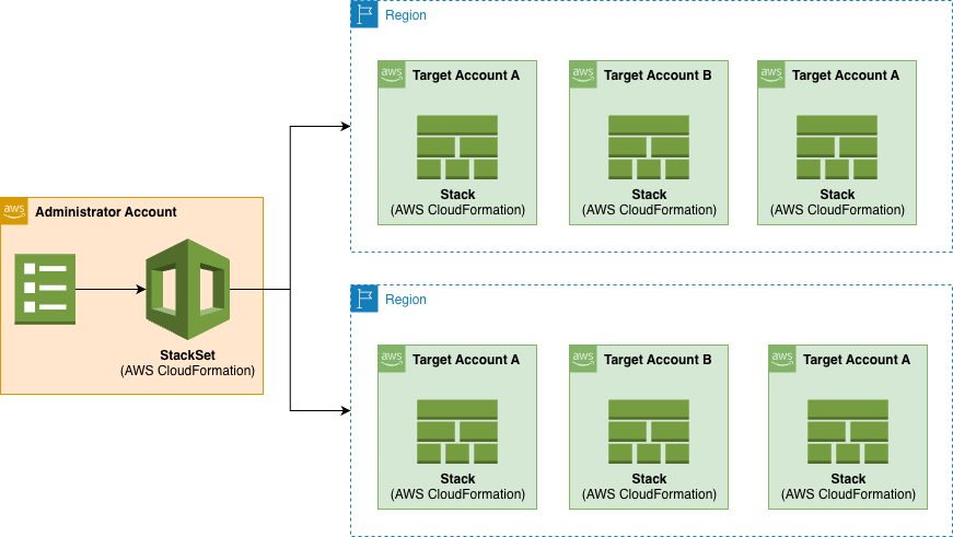
Post Syndicated from Amar Meriche original https://aws.amazon.com/blogs/devops/stacksets-deployment-strategies-balancing-speed-safety-and-scale-to-optimize-deployments-for-different-organizational-needs/
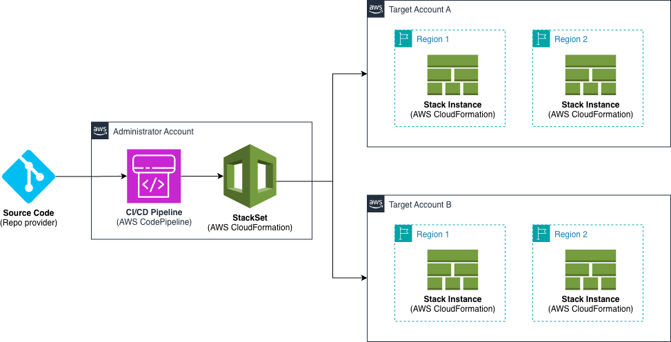
AWS CloudFormation StackSets enables organizations to deploy infrastructure consistently across multiple AWS accounts and regions. However, success depends on choosing the right deployment strategy that balances three critical factors: deployment speed, operational safety, and organizational scale. This guide explores proven StackSets deployment strategies specifically designed for multi-account infrastructure management.
Understanding StackSets Deployment Fundamentals
What are StackSets Actually Used For?
Unlike single-account AWS CloudFormation templates, StackSets are specifically designed for multi-account infrastructure governance. Common use cases include Security baselines (deploying IAM policies, security groups, and access controls across all accounts), Compliance controls (rolling out AWS Config rules, AWS CloudTrail configurations, and audit requirements), Organizational standards (establishing consistent VPC configurations, tagging policies, and naming conventions), Shared services (deploying monitoring solutions, logging infrastructure, and backup policies) or Cost management (implementing budget controls, cost allocation tags, and resource optimization policies)
The Multi-Account Challenge
Managing infrastructure across dozens or hundreds of AWS accounts presents unique challenges:
Single Account (CFN Template) Multi-Account (StackSets)
App A Org Unit A (50 accounts)
| |
[Deploy Once] [Deploy consistently across all]
| |
Success/Fail Complex success/failure matrix
Multi account and multi region Cloudformation deployment complexity
The Speed-Safety-Scale Triangle
Every StackSets deployment strategy involves trade-offs: Speed (how quickly changes propagate across your organization), Safety (risk mitigation and failure containment) and Scale (ability to manage hundreds of accounts efficiently)
Prerequisites
Before implementing any of the deployment strategies described in this guide, ensure you have:
- AWS CLI Installation
- Install the latest version of AWS CLI by following the AWS CLI installation guide
- Verify installation with: aws –version
- AWS Profile Configuration
- Configure your AWS credentials using: aws configure
- For details on configuration, see AWS CLI configuration basics
- Ensure your profile has appropriate permissions for CloudFormation StackSets operations as described in AWS StackSets prerequisites
- Proper Account Access The commands in this guide must be executed from either:
- The management account of your AWS Organization
- OR a delegated administrator account for CloudFormation
For information on setting up a delegated administrator, see Register a delegated administrator
Note: StackSets deployments using service-managed permissions cannot be performed from standalone accounts.
Verify you’re using the correct account with:
bash
# For management account
aws organizations describe-organization
# For delegated admin
aws cloudformation list-stack-sets —call-as DELEGATED_ADMIN
AWS CLI to check the usage of an Organization and not a Standalone account
Core Deployment Strategies
As explained in the StackSet documentation:
- “For a more conservative deployment, set Maximum Concurrent Accounts to 1, and Failure Tolerance to 0. Set your lowest-impact region to be first in the Region Order Start with one region.”
- “For a faster deployment, increase the values of Maximum Concurrent Accounts and Failure Tolerance as needed. ”
Based on the above, we are proposing below several deployment strategies, depending on the speed, safety and scale you want to achieve.
1. Sequential Deployment: Maximum Safety
Use Case : Critical security updates, compliance requirements, first-time organizational rollouts
Below are listed some possible use cases:
- Security baseline updates: New IAM policies affecting root access
- Compliance rollouts: SOX, HIPAA, or PCI-DSS control implementations
- Critical infrastructure changes: VPC security group modifications
- Organizational policy changes: New AWS Config rules for audit compliance
Implementation Example:
For this example, we will download the following template ConfigRuleCloudtrailEnabled.yml from the Cloudformation sample library in the AWS documentation to configure an AWS Config rule to determine if AWS CloudTrail is enabled and follow the next steps:
Step 1: Create the StackSet
With the AWS CLI:
# Create Stackset for security baseline
# StackSet operation managed from us-east-1
aws cloudformation create-stack-set \
--stack-set-name security-baseline \
--template-body file://ConfigRuleCloudtrailEnabled.yml \
--capabilities CAPABILITY_NAMED_IAM \
--permission-model SERVICE_MANAGED \
--auto-deployment Enabled=true,RetainStacksOnAccountRemoval=false \
--region us-east-1
AWS CLI to create a security-baseline Stackset
The expected response should be similar to the following :
{"StacksetId": "security-baseline: ...."}
Step 2: Create Stack Instances
Before you launch the below command, you need to adjust the values of the following parameters:
- OrganizationalUnitIds: you must change the value “ou-test” in the below command line to the name of the target OU you want to deploy to. I recommend creating a new test OU in the console or via the CLI for the purpose of this test.
- regions: if needed, change the “us-east-1 eu-west-1” value, here you need to list all the regions you want to deploy to. AWS Config must be active in the accounts/regions that you choose, otherwise you’ll get an error when deploying the Stack.
# Deploy security baseline to production accounts
# StackSet operation managed from us-east-1
# Deployed to regions us-east-1 and eu-west-1
# SEQUENTIAL = One region at a time, sequentially
# MaxConcurrentPercentage = Deploy to 5% of accounts at once
# FailureTolerancePercentage = Stop on first failure
aws cloudformation create-stack-instances \
--stack-set-name security-baseline \
--deployment-targets OrganizationalUnitIds=ou-test\
--regions us-east-1 eu-west-1 \
--region us-east-1 \
--operation-preferences RegionConcurrencyType=SEQUENTIAL,MaxConcurrentPercentage=5,FailureTolerancePercentage=0
AWS CLI to create security-baseline Stack Instances sequentially for maximum safety
The CLI output should look like the following:
{"OperationId": ....}
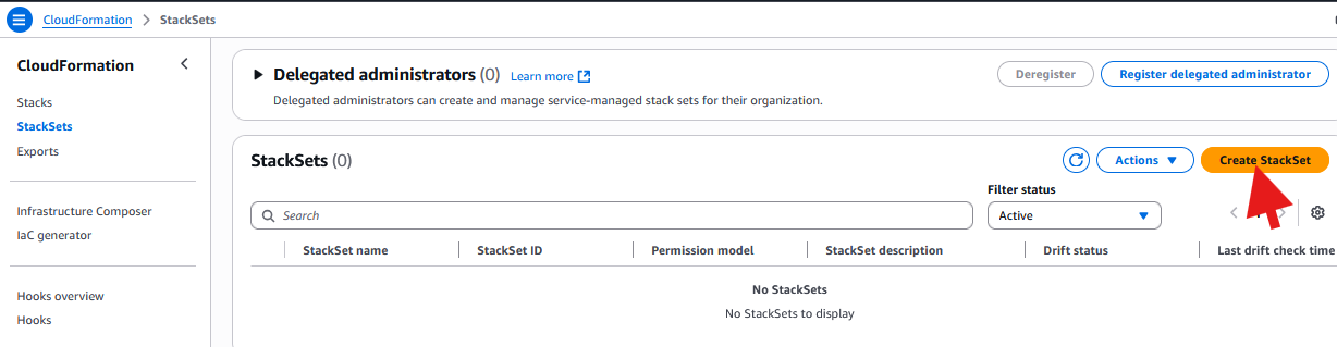
Or create the StackSet and add the Stacks with the AWS Console:
In the CloudFormation Console, click “Create StackSet”

AWS CloudFormation Console: create a security-baseline Stackset
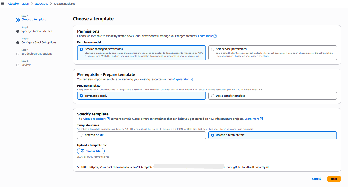
Upload your template from S3 or from your computer and click Next:

AWS CloudFormation Console: specify a template
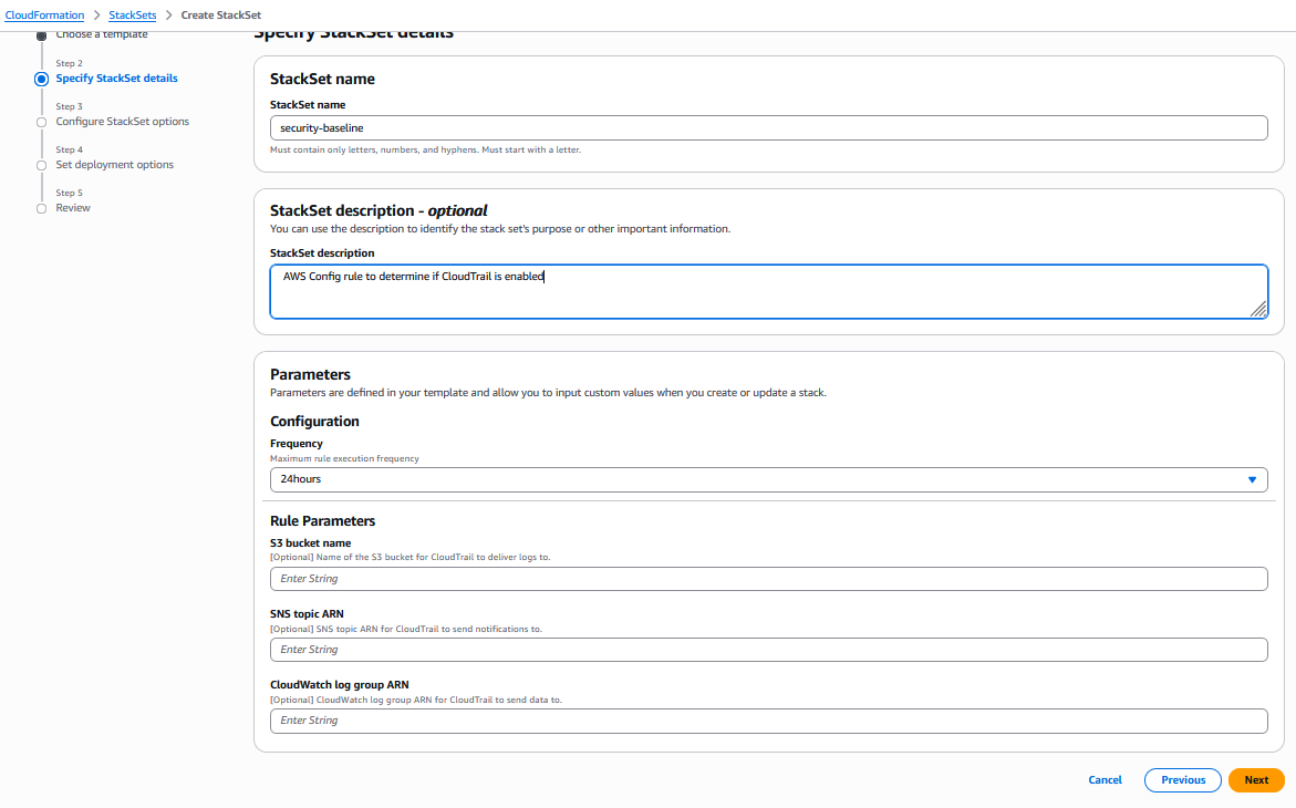
Specify the StackSet name and parameters and click Next:

AWS CloudFormation Console: specify the StackSet name and parameters
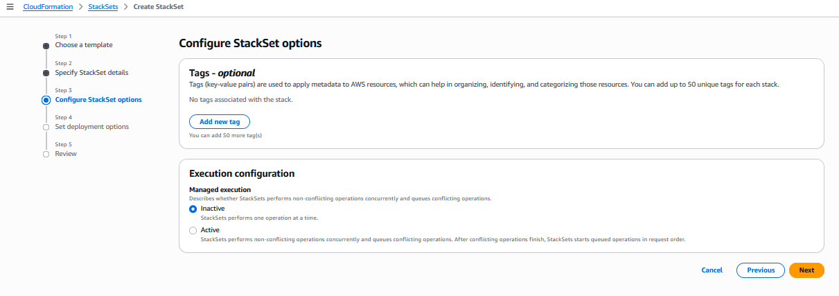
Configure StackSet options and click Next:

AWS CloudFormation Console: configure the StackSet options
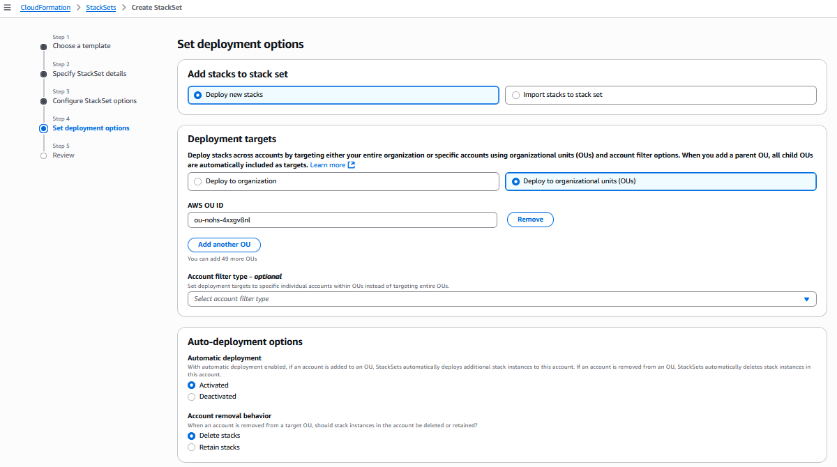
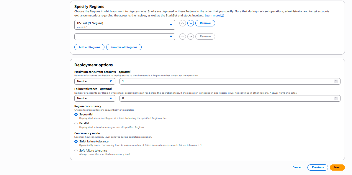
Set deployment options and click Next:

AWS CloudFormation Console: set deployment options

AWS CloudFormation Console: set more deployment options
Then Review and Submit.
Not to overweight this blog, we’ll provide only this example of CLI output and Console screenshot, but the “Parallel Deployment” and “Balanced Approach” will be similar to this example. You just need to update the parameters for the different StackSet Operations options.
A real-world example would be a financial services company deploying new MFA requirements across 200 production accounts. They could use sequential deployment with 5 concurrency to ensure each batch was validated before proceeding.
2. Parallel Deployment: Maximum Speed
The Parallel Deployment is best for non-critical updates, development environments, routine maintenance
Here are some possible use cases:
- Development account standardization: Rolling out new development tools
- Monitoring infrastructure: Deploying Amazon CloudWatch dashboards and alarms
- Cost optimization: Implementing automated resource cleanup policies
- Non-production updates: Updating development and staging environments
Implementation Example:
For this example, we will copy paste the .yml template from this Re:Post article about monitoring IAM events in a file called “monitoring-baseline.yml”, and use it in the following command lines.
Step 1: Create the StackSet
# Create Stackset for monitoring baseline
# StackSet operation managed from us-east-1
aws cloudformation create-stack-set \
--stack-set-name monitoring-baseline \
--template-body file://monitoring-baseline.yml \
--capabilities CAPABILITY_NAMED_IAM \
--permission-model SERVICE_MANAGED \
--auto-deployment Enabled=true,RetainStacksOnAccountRemoval=false \
--region us-east-1
AWS CLI to create a monitoring-baseline Stackset
Step 2: Create Stack Instances
Just like in the previous example, before you launch the below command, you need to adjust the values of the OrganizationalUnitIds and regions parameters.
# Deploy monitoring baseline to dev and sandbox accounts
# StackSet operation managed from us-east-1
# Deployed to regions us-east-1 and eu-west-1
# PARALLEL = Deployment in parallel
# MaxConcurrentPercentage = Deploy to 80% of accounts at once
# FailureTolerancePercentage = Tolerate failures in 20% of accounts
aws cloudformation create-stack-instances \
--stack-set-name monitoring-baseline \
--deployment-targets OrganizationalUnitIds=ou-development,ou-sandbox \
--regions us-east-1 eu-west-1 \
--region us-east-1 \
--operation-preferences RegionConcurrencyType=PARALLEL,MaxConcurrentPercentage=80,FailureTolerancePercentage=20
AWS CLI to create monitoring-baseline Stack Instances in parallel with high value for max concurrent percentage for maximum speed
3. Progressive Deployment: Balanced Approach or Multi Phase Approach (Recommended)
For most production scenarios with moderate risk tolerance, it is recommended to use a Balanced Approach, or Multi-Phase Implementation.
Balanced Approach
For this example, to make it easier, you can create a copy of “monitoring-baseline.yml” created previously, and name it “balanced-template.yml”.
cp monitoring-baseline.yml balanced-template.yml
bash command to copy the monitoring-baseline.yml file to balanced-template.yml
Then you can use it in the following command lines.
Step 1: Create the StackSet
# Create Stackset for a balanced creation
# StackSet operation managed from us-east-1
aws cloudformation create-stack-set \
--stack-set-name balanced-deployment \
--template-body file://balanced-template.yml \
--capabilities CAPABILITY_NAMED_IAM \
--permission-model SERVICE_MANAGED \
--auto-deployment Enabled=true,RetainStacksOnAccountRemoval=false \
--region us-east-1
AWS CLI to create a balanced-deployment Stackset
Step 2: Create Stack Instances
You need to adjust the values of the OrganizationalUnitIds and regions parameters.
# Deploy monitoring baseline to production accounts
# StackSet operation managed from us-east-1
# Deployed to regions us-east-1, eu-west-1 and ap-southeast-1
# PARALLEL = Deployment in parallel
# MaxConcurrentPercentage = Deploy to 25% of accounts at once
# FailureTolerancePercentage = Tolerate failures in 8% of accounts
aws cloudformation create-stack-instances \
--stack-set-name balanced-deployment \
--deployment-targets OrganizationalUnitIds=ou-development,ou-sandbox \
--regions us-east-1 eu-west-1 ap-southeast-1 \
--region us-east-1 \
--operation-preferences RegionConcurrencyType=PARALLEL,MaxConcurrentPercentage=25,FailureTolerancePercentage=8
AWS CLI to create balanced-deployment Stack Instances in parallel with low max concurrent percentage for a balanced deployment
Multi-Phase Implementation:
Step 1: Create the StackSet
# Create Stackset for a balanced creation
# StackSet operation managed from us-east-1
aws cloudformation create-stack-set \
--stack-set-name balanced-deployment \
--template-body file://balanced-template.yml \
--capabilities CAPABILITY_NAMED_IAM \
--permission-model SERVICE_MANAGED \
--auto-deployment Enabled=true,RetainStacksOnAccountRemoval=false \
--region us-east-1
AWS CLI to create a balanced-deployment Stackset
Phase 1: Pilot Accounts (10% of target)
Phase 1: Create Pilot Stack Instances
You need to adjust the values of the OrganizationalUnitIds and regions parameters.
# Deploy monitoring baseline to production accounts
# StackSet operation managed from us-east-1
# Deployed to regions us-east-1
# SEQUENTIAL = Deployment in sequence
# MaxConcurrentPercentage = 100% Deploy full speed for small pilot
# FailureTolerancePercentage = Zero tolerance in pilot
aws cloudformation create-stack-instances \
--stack-set-name balanced-deployment \
--deployment-targets Accounts=pilot-account-1,pilot-account-2 \
--regions us-east-1 \
--region us-east-1 \
--operation-preferences RegionConcurrencyType=SEQUENTIAL,MaxConcurrentPercentage=100,FailureTolerancePercentage=0
AWS CLI to create balanced-deployment Stack Instances sequentially for maximum safety in Pilot accounts
Wait for Pilot validation before proceeding to Phase 2
Phase 2: Early Adopter OUs (30% of target)
Phase 2: Create Early Adopter Stack Instances
You need to adjust the values of the OrganizationalUnitIds and regions parameters.
# Deploy monitoring baseline to production accounts
# StackSet operation managed from us-east-1
# Deployed to regions us-east-1, eu-west-1
# PARALLEL = Deployment in parallel
# MaxConcurrentPercentage = Deploy to 25% of accounts at once
# FailureTolerancePercentage = Tolerate failures in 5% of accounts
aws cloudformation create-stack-instances \
--stack-set-name balanced-deployment \
--deployment-targets OrganizationalUnitIds=ou-early-adopter \
--regions us-east-1 \
--region us-east-1 eu-west-1 \
--operation-preferences RegionConcurrencyType=PARALLEL,MaxConcurrentPercentage=25,FailureTolerancePercentage=5
AWS CLI to create balanced-deployment Stack Instances in parallel with low max concurrent percentage for a balanced deployment in Early Adopter OU
Wait for Early Adopter validation before proceeding to Phase 3
Phase 3: Full Deployment (Remaining 60%)
Phase 3: Full Deployment
You need to adjust the values of the OrganizationalUnitIds and regions parameters.
# Deploy monitoring baseline to production accounts
# StackSet operation managed from us-east-1
# Deployed to regions us-east-1, eu-west-1 and ap-southeast-1
# PARALLEL = Deployment in parallel
# MaxConcurrentPercentage = Deploy to 40% of accounts at once for higher speed after validation
# FailureTolerancePercentage = Tolerate failures in 10% of accounts for moderate tolerance
aws cloudformation create-stack-instances \
--stack-set-name balanced-deployment \
--deployment-targets OrganizationalUnitIds=ou-standard-prod,ou-legacy-prod \
--regions us-east-1 \
--region us-east-1 eu-west-1 ap-southeast-1 \
--operation-preferences RegionConcurrencyType=PARALLEL,MaxConcurrentPercentage=25,FailureTolerancePercentage=5
AWS CLI to create balanced-deployment Stack Instances in parallel with low max concurrent percentage for a balanced deployment in the remaining OUs
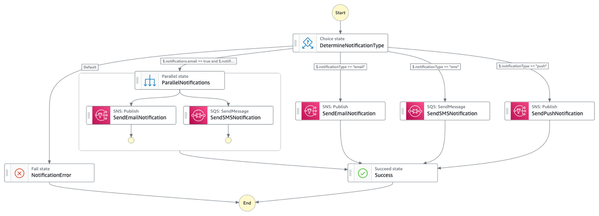
Using Step Functions for Orchestration
AWS Step Functions provides a serverless workflow service that can orchestrate StackSets deployments with advanced control flow, error handling, and state management capabilities. This approach enhances your multi-account deployments with features not available through standard StackSets operations alone.
Some of the Key Benefits include:
- Advanced Deployment Orchestration: Coordinate multi-phase rollouts with validation gates
- Human Approval Workflows: Implement manual approval steps for critical changes
- Enhanced Error Handling: Define sophisticated retry policies and fallback mechanisms
- Visual Monitoring: Track deployment progress through the Step Functions visual console
Real-World Use Case: Compliance Control Rollout
In regulated industries, AWS Step Functions enables a phased approach that combines automation with necessary governance. For instance, you can:
- Deploy compliance controls to test accounts
- Run automated validation and generate compliance reports
- Obtain manual approval from compliance team
- Deploy to production accounts with comprehensive monitoring
This approach ensures consistent governance while maintaining the complete audit trail required for regulatory compliance.
Monitoring and Optimization
AWS CloudFormation StackSets do not have extensive built-in Amazon CloudWatch metrics specifically designed for monitoring StackSet operations and health. This is actually why the monitoring implementation in our blog post is valuable.
Here’s what AWS does and doesn’t provide out of the box:
What AWS provides natively:
- Basic AWS API call metrics via AWS CloudTrail (which show that operations happened but don’t track success rates or performance)
- General service quotas and throttling metrics for CloudFormation as a whole
- CloudFormation provides some metrics for individual stacks, but not consolidated StackSet-specific metrics
What requires custom implementation (as in our blog post):
- Success rate metrics for StackSet operations across accounts
- Deployment completion time tracking
- Configuration drift detection and monitoring
- Account-specific failure analysis
- Comprehensive dashboards that show StackSet health across your organization
The code in our blog post demonstrates how to implement the success rate custom metrics by:
- Gathering data from the CloudFormation API about StackSet operations
- Calculating the success rate metrics for StackSet deployments
- Creating custom Amazon CloudWatch metrics in a custom namespace (like “StackSetMonitoring”)
- Setting up alerts for issues
This explains why organizations need to implement custom monitoring solutions like the one shown in our blog post rather than relying solely on built-in metrics.
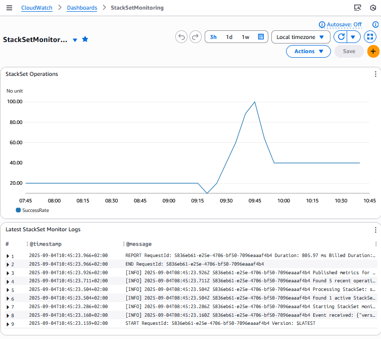
Automated Monitoring Implementation: example of a custom metric to monitor the StackSet operations success rate
The following AWS Cloudformation template provides real-time monitoring and alerting for AWS CloudFormation StackSet operations through automated infrastructure deployment. This solution creates a complete monitoring system using a AWS Lambda function, Amazon EventBridge rules, Amazon SNS notifications, and Amazon CloudWatch dashboards to track StackSet success and failure rates. The core Lambda function named StackSetMonitor continuously monitors all active StackSets in your account, calculating success rates and publishing custom metrics to Amazon CloudWatch under the StackSetMonitoring namespace.
Below you’ll find a few example of possible custom metrics that could be implemented based on this AWS Cloudformation template:
- Count of all operations (CREATE, UPDATE, DELETE) per StackSet over time periods
- Number of stack instances with configuration drift (requires additional API calls)
- Average time taken for StackSet operations to complete
- Rate of StackSet operations to identify peak usage times
- Number of individual stack instances that failed during operations
- Number of retried operations (indicates infrastructure issues)
- …
Here’s the StackSetMonitor.yml CloudFormation Template:
# StackSetMonitor.yml
# CFN template for monitoring AWS CloudFormation StackSet operations with real-time alerts, metrics, and dashboards.
AWSTemplateFormatVersion: '2010-09-09'
Description: 'CloudFormation template for StackSet operation monitoring using CloudWatch and SNS'
Parameters:
StackSetName:
Type: String
Description: 'Name of the StackSet to monitor'
Default: 'security-baseline'
MinLength: 1
MaxLength: 128
AllowedPattern: '[a-zA-Z][-a-zA-Z0-9]*'
ConstraintDescription: 'Must be a valid StackSet name (1-128 characters, alphanumeric and hyphens, must start with a letter)'
VpcId:
Type: String
Description: 'VPC ID where the Lambda function will be deployed (leave empty to create new VPC)'
Default: ''
SubnetIds:
Type: CommaDelimitedList
Description: 'List of subnet IDs for the Lambda function (leave empty to create new subnets)'
Default: ''
SecurityGroupIds:
Type: CommaDelimitedList
Description: 'List of security group IDs for the Lambda function (leave empty to create new security group)'
Default: ''
Conditions:
CreateVPC: !Equals [!Ref VpcId, '']
CreateVPCAndSubnets: !And [!Equals [!Ref VpcId, ''], !Equals [!Join [',', !Ref SubnetIds], '']]
HasCustomSecurityGroups: !Not [!Equals [!Join [',', !Ref SecurityGroupIds], '']]
Resources:
# KMS Key for CloudWatch Logs encryption
LogsKMSKey:
Type: AWS::KMS::Key
DeletionPolicy: Delete
UpdateReplacePolicy: Delete
Properties:
Description: 'KMS Key for StackSet Monitor CloudWatch Logs and Lambda environment variable encryption'
EnableKeyRotation: true
KeyPolicy:
Version: '2012-10-17'
Statement:
- Sid: Enable IAM User Permissions
Effect: Allow
Principal:
AWS: !Sub 'arn:${AWS::Partition}:iam::${AWS::AccountId}:root'
Action: 'kms:*'
Resource: '*'
- Sid: Allow CloudWatch Logs
Effect: Allow
Principal:
Service: !Sub 'logs.${AWS::Region}.amazonaws.com'
Action:
- 'kms:Encrypt'
- 'kms:Decrypt'
- 'kms:ReEncrypt*'
- 'kms:GenerateDataKey*'
- 'kms:DescribeKey'
Resource: '*'
Condition:
ArnEquals:
'kms:EncryptionContext:aws:logs:arn':
- !Sub 'arn:${AWS::Partition}:logs:${AWS::Region}:${AWS::AccountId}:log-group:/aws/lambda/StackSetMonitor'
- !Sub 'arn:${AWS::Partition}:logs:${AWS::Region}:${AWS::AccountId}:log-group:/aws/cloudformation/stacksets'
- Sid: Allow Lambda Service
Effect: Allow
Principal:
Service: lambda.amazonaws.com
Action:
- 'kms:Encrypt'
- 'kms:Decrypt'
- 'kms:ReEncrypt*'
- 'kms:GenerateDataKey*'
- 'kms:DescribeKey'
Resource: '*'
LogsKMSKeyAlias:
Type: AWS::KMS::Alias
Properties:
AliasName: alias/stackset-monitor-logs
TargetKeyId: !Ref LogsKMSKey
# VPC Resources (created when no existing VPC is provided)
StackSetMonitorVPC:
Type: AWS::EC2::VPC
Condition: CreateVPC
Properties:
CidrBlock: 10.0.0.0/16
EnableDnsHostnames: true
EnableDnsSupport: true
Tags:
- Key: Name
Value: StackSetMonitor-VPC
- Key: Purpose
Value: VPC for StackSet Monitor Lambda function
PrivateSubnet1:
Type: AWS::EC2::Subnet
Condition: CreateVPC
Properties:
VpcId: !Ref StackSetMonitorVPC
CidrBlock: 10.0.1.0/24
AvailabilityZone: !Select [0, !GetAZs '']
Tags:
- Key: Name
Value: StackSetMonitor-Private-Subnet-1
- Key: Purpose
Value: Private subnet for StackSet Monitor Lambda
PrivateSubnet2:
Type: AWS::EC2::Subnet
Condition: CreateVPC
Properties:
VpcId: !Ref StackSetMonitorVPC
CidrBlock: 10.0.2.0/24
AvailabilityZone: !Select [1, !GetAZs '']
Tags:
- Key: Name
Value: StackSetMonitor-Private-Subnet-2
- Key: Purpose
Value: Private subnet for StackSet Monitor Lambda
PrivateRouteTable1:
Type: AWS::EC2::RouteTable
Condition: CreateVPC
Properties:
VpcId: !Ref StackSetMonitorVPC
Tags:
- Key: Name
Value: StackSetMonitor-Private-RT-1
PrivateRouteTable2:
Type: AWS::EC2::RouteTable
Condition: CreateVPC
Properties:
VpcId: !Ref StackSetMonitorVPC
Tags:
- Key: Name
Value: StackSetMonitor-Private-RT-2
PrivateSubnet1RouteTableAssociation:
Type: AWS::EC2::SubnetRouteTableAssociation
Condition: CreateVPC
Properties:
RouteTableId: !Ref PrivateRouteTable1
SubnetId: !Ref PrivateSubnet1
PrivateSubnet2RouteTableAssociation:
Type: AWS::EC2::SubnetRouteTableAssociation
Condition: CreateVPC
Properties:
RouteTableId: !Ref PrivateRouteTable2
SubnetId: !Ref PrivateSubnet2
# VPC Endpoints for AWS Services (no internet access needed)
CloudFormationVPCEndpoint:
Type: AWS::EC2::VPCEndpoint
Condition: CreateVPC
Properties:
VpcId: !Ref StackSetMonitorVPC
ServiceName: !Sub com.amazonaws.${AWS::Region}.cloudformation
VpcEndpointType: Interface
SubnetIds:
- !Ref PrivateSubnet1
- !Ref PrivateSubnet2
SecurityGroupIds:
- !Ref VPCEndpointSecurityGroup
PrivateDnsEnabled: true
PolicyDocument:
Version: '2012-10-17'
Statement:
- Effect: Allow
Principal: '*'
Action:
- cloudformation:ListStackSets
- cloudformation:ListStackSetOperations
- cloudformation:ListStackInstances
- cloudformation:DescribeStackInstance
- cloudformation:DescribeStacks
- cloudformation:GetTemplate
Resource: '*'
CloudWatchVPCEndpoint:
Type: AWS::EC2::VPCEndpoint
Condition: CreateVPC
Properties:
VpcId: !Ref StackSetMonitorVPC
ServiceName: !Sub com.amazonaws.${AWS::Region}.monitoring
VpcEndpointType: Interface
SubnetIds:
- !Ref PrivateSubnet1
- !Ref PrivateSubnet2
SecurityGroupIds:
- !Ref VPCEndpointSecurityGroup
PrivateDnsEnabled: true
PolicyDocument:
Version: '2012-10-17'
Statement:
- Effect: Allow
Principal: '*'
Action:
- cloudwatch:PutMetricData
Resource: '*'
SNSVPCEndpoint:
Type: AWS::EC2::VPCEndpoint
Condition: CreateVPC
Properties:
VpcId: !Ref StackSetMonitorVPC
ServiceName: !Sub com.amazonaws.${AWS::Region}.sns
VpcEndpointType: Interface
SubnetIds:
- !Ref PrivateSubnet1
- !Ref PrivateSubnet2
SecurityGroupIds:
- !Ref VPCEndpointSecurityGroup
PrivateDnsEnabled: true
PolicyDocument:
Version: '2012-10-17'
Statement:
- Effect: Allow
Principal: '*'
Action:
- sns:Publish
Resource: '*'
EventsVPCEndpoint:
Type: AWS::EC2::VPCEndpoint
Condition: CreateVPC
Properties:
VpcId: !Ref StackSetMonitorVPC
ServiceName: !Sub com.amazonaws.${AWS::Region}.events
VpcEndpointType: Interface
SubnetIds:
- !Ref PrivateSubnet1
- !Ref PrivateSubnet2
SecurityGroupIds:
- !Ref VPCEndpointSecurityGroup
PrivateDnsEnabled: true
PolicyDocument:
Version: '2012-10-17'
Statement:
- Effect: Allow
Principal: '*'
Action:
- events:PutEvents
Resource: '*'
LogsVPCEndpoint:
Type: AWS::EC2::VPCEndpoint
Condition: CreateVPC
Properties:
VpcId: !Ref StackSetMonitorVPC
ServiceName: !Sub com.amazonaws.${AWS::Region}.logs
VpcEndpointType: Interface
SubnetIds:
- !Ref PrivateSubnet1
- !Ref PrivateSubnet2
SecurityGroupIds:
- !Ref VPCEndpointSecurityGroup
PrivateDnsEnabled: true
PolicyDocument:
Version: '2012-10-17'
Statement:
- Effect: Allow
Principal: '*'
Action:
- logs:CreateLogGroup
- logs:CreateLogStream
- logs:PutLogEvents
Resource: '*'
SQSVPCEndpoint:
Type: AWS::EC2::VPCEndpoint
Condition: CreateVPC
Properties:
VpcId: !Ref StackSetMonitorVPC
ServiceName: !Sub com.amazonaws.${AWS::Region}.sqs
VpcEndpointType: Interface
SubnetIds:
- !Ref PrivateSubnet1
- !Ref PrivateSubnet2
SecurityGroupIds:
- !Ref VPCEndpointSecurityGroup
PrivateDnsEnabled: true
PolicyDocument:
Version: '2012-10-17'
Statement:
- Effect: Allow
Principal: '*'
Action:
- sqs:SendMessage
Resource: '*'
STSVPCEndpoint:
Type: AWS::EC2::VPCEndpoint
Condition: CreateVPC
Properties:
VpcId: !Ref StackSetMonitorVPC
ServiceName: !Sub com.amazonaws.${AWS::Region}.sts
VpcEndpointType: Interface
SubnetIds:
- !Ref PrivateSubnet1
- !Ref PrivateSubnet2
SecurityGroupIds:
- !Ref VPCEndpointSecurityGroup
PrivateDnsEnabled: true
PolicyDocument:
Version: '2012-10-17'
Statement:
- Effect: Allow
Principal: '*'
Action:
- sts:AssumeRole
- sts:GetCallerIdentity
- sts:AssumeRoleWithWebIdentity
Resource: '*'
# Security Group for Lambda function
LambdaSecurityGroup:
Type: AWS::EC2::SecurityGroup
Properties:
GroupDescription: Security group for StackSet Monitor Lambda function
VpcId: !If
- CreateVPC
- !Ref StackSetMonitorVPC
- !Ref VpcId
SecurityGroupEgress:
- IpProtocol: tcp
FromPort: 443
ToPort: 443
CidrIp: 10.0.0.0/16
Description: HTTPS to VPC Endpoints
- IpProtocol: tcp
FromPort: 53
ToPort: 53
CidrIp: 10.0.0.0/16
Description: DNS TCP to VPC for name resolution
- IpProtocol: udp
FromPort: 53
ToPort: 53
CidrIp: 10.0.0.0/16
Description: DNS UDP to VPC for name resolution
Tags:
- Key: Name
Value: StackSetMonitor-Lambda-SG
- Key: Purpose
Value: Security group for StackSet Monitor Lambda
VPCEndpointSecurityGroup:
Type: AWS::EC2::SecurityGroup
Condition: CreateVPC
Properties:
GroupDescription: Security group for VPC Endpoints
VpcId: !Ref StackSetMonitorVPC
SecurityGroupIngress:
- IpProtocol: tcp
FromPort: 443
ToPort: 443
SourceSecurityGroupId: !Ref LambdaSecurityGroup
Description: HTTPS from Lambda security group
- IpProtocol: tcp
FromPort: 53
ToPort: 53
SourceSecurityGroupId: !Ref LambdaSecurityGroup
Description: DNS TCP from Lambda security group
- IpProtocol: udp
FromPort: 53
ToPort: 53
SourceSecurityGroupId: !Ref LambdaSecurityGroup
Description: DNS UDP from Lambda security group
SecurityGroupEgress:
- IpProtocol: tcp
FromPort: 443
ToPort: 443
CidrIp: 10.0.0.0/16
Description: HTTPS outbound within VPC
- IpProtocol: tcp
FromPort: 53
ToPort: 53
CidrIp: 10.0.0.0/16
Description: DNS TCP outbound within VPC
- IpProtocol: udp
FromPort: 53
ToPort: 53
CidrIp: 10.0.0.0/16
Description: DNS UDP outbound within VPC
Tags:
- Key: Name
Value: StackSetMonitor-VPCEndpoint-SG
- Key: Purpose
Value: Security group for VPC Endpoints
# Dead Letter Queue for Lambda function
StackSetMonitorDLQ:
Type: AWS::SQS::Queue
DeletionPolicy: Delete
UpdateReplacePolicy: Delete
Properties:
QueueName: StackSetMonitor-DLQ
MessageRetentionPeriod: 1209600 # 14 days
KmsMasterKeyId: alias/aws/sqs
Tags:
- Key: Purpose
Value: Dead Letter Queue for StackSet Monitor Lambda
StackSetAlertsTopic:
Type: AWS::SNS::Topic
Properties:
TopicName: StackSetAlerts
DisplayName: StackSet Monitoring Alerts
KmsMasterKeyId: alias/aws/sns
StackSetLogGroup:
Type: AWS::Logs::LogGroup
DeletionPolicy: Delete
UpdateReplacePolicy: Delete
Properties:
LogGroupName: /aws/cloudformation/stacksets
RetentionInDays: 30
KmsKeyId: !GetAtt LogsKMSKey.Arn
LambdaLogGroup:
Type: AWS::Logs::LogGroup
DeletionPolicy: Delete
UpdateReplacePolicy: Delete
Properties:
LogGroupName: /aws/lambda/StackSetMonitor
RetentionInDays: 30
KmsKeyId: !GetAtt LogsKMSKey.Arn
StackSetMonitoringDashboard:
Type: AWS::CloudWatch::Dashboard
Properties:
DashboardName: StackSetMonitoring
DashboardBody: !Sub |
{
"widgets": [
{
"type": "metric",
"width": 24,
"height": 8,
"properties": {
"metrics": [
[ "StackSetMonitoring", "SuccessRate", "StackSetName", "${StackSetName}" ]
],
"region": "${AWS::Region}",
"title": "StackSet Operations",
"period": 300,
"stat": "Average"
}
},
{
"type": "log",
"width": 24,
"height": 6,
"properties": {
"query": "SOURCE '/aws/lambda/StackSetMonitor' | fields @timestamp, @message\n| sort @timestamp desc\n| limit 20",
"region": "${AWS::Region}",
"title": "Latest StackSet Monitor Logs",
"view": "table"
}
}
]
}
# Consolidated rule to catch ALL StackSet events for comprehensive monitoring
AllStackSetOperationsRule:
Type: AWS::Events::Rule
Properties:
Name: AllStackSetOperationsRule
Description: "Rule for monitoring all CloudFormation StackSet operations with failure notifications"
EventPattern: {source: ["aws.cloudformation"], detail-type: ["CloudFormation StackSet Operation Status Change"]}
State: ENABLED
Targets:
- Id: ProcessAllEvents
Arn: !GetAtt StackSetMonitorLambda.Arn
- Id: NotifyFailure
Arn: !Ref StackSetAlertsTopic
InputTransformer:
InputPathsMap:
"stackSetId": "$.detail.stack-set-id"
"operationId": "$.detail.operation-id"
"status": "$.detail.status"
"time": "$.time"
InputTemplate: '"StackSet Event: ID: <stackSetId>, Op: <operationId>, Status: <status>, Time: <time>"'
StackSetMonitorLambda:
Type: AWS::Lambda::Function
DependsOn: LambdaLogGroup
Properties:
FunctionName: StackSetMonitor
Handler: index.lambda_handler
Role: !GetAtt StackSetMonitorRole.Arn
Runtime: python3.12
Timeout: 300
MemorySize: 512
ReservedConcurrentExecutions: 1
DeadLetterConfig:
TargetArn: !GetAtt StackSetMonitorDLQ.Arn
VpcConfig:
SecurityGroupIds: !If
- HasCustomSecurityGroups
- !Ref SecurityGroupIds
- - !Ref LambdaSecurityGroup
SubnetIds: !If
- CreateVPCAndSubnets
- - !Ref PrivateSubnet1
- !Ref PrivateSubnet2
- !Ref SubnetIds
KmsKeyArn: !GetAtt LogsKMSKey.Arn
Code:
ZipFile: |
import boto3
import json
import os
import logging
import time
import datetime
from typing import Dict, Any, Optional
# Custom JSON encoder to handle datetime objects
class DateTimeEncoder(json.JSONEncoder):
def default(self, obj):
if isinstance(obj, datetime.datetime):
return obj.isoformat()
return super().default(obj)
# Set up logging with more details
logger = logging.getLogger()
logger.setLevel(logging.INFO)
# Log initialization to verify Lambda is loading correctly
print("StackSetMonitor Lambda initializing...")
def validate_event(event: Dict[str, Any]) -> bool:
"""Validate the incoming event structure"""
if not isinstance(event, dict):
logger.error("Event must be a dictionary")
return False
# If it's an EventBridge event, validate required fields
if 'detail' in event:
detail = event.get('detail', {})
if not isinstance(detail, dict):
logger.error("Event detail must be a dictionary")
return False
# Validate StackSet event structure
if 'stack-set-id' in detail:
stack_set_id = detail.get('stack-set-id')
if not isinstance(stack_set_id, str) or not stack_set_id.strip():
logger.error("stack-set-id must be a non-empty string")
return False
# Validate operation-id if present
operation_id = detail.get('operation-id')
if operation_id is not None and not isinstance(operation_id, str):
logger.error("operation-id must be a string if provided")
return False
# Validate status if present
status = detail.get('status')
if status is not None and not isinstance(status, str):
logger.error("status must be a string if provided")
return False
return True
def validate_context(context: Any) -> bool:
"""Validate the Lambda context object"""
if context is None:
logger.error("Context cannot be None")
return False
# Check for required context attributes
required_attrs = ['function_name', 'function_version', 'invoked_function_arn', 'memory_limit_in_mb']
for attr in required_attrs:
if not hasattr(context, attr):
logger.error(f"Context missing required attribute: {attr}")
return False
return True
def sanitize_string(value: str, max_length: int = 255) -> str:
"""Sanitize and truncate string inputs"""
if not isinstance(value, str):
return str(value)[:max_length]
return value.strip()[:max_length]
def lambda_handler(event: Dict[str, Any], context: Any) -> Dict[str, Any]:
"""Main Lambda handler function for StackSet monitoring with input validation"""
# Input validation
if not validate_event(event):
return {
"statusCode": 400,
"body": json.dumps({
"status": "error",
"message": "Invalid event structure"
}, cls=DateTimeEncoder)
}
if not validate_context(context):
return {
"statusCode": 400,
"body": json.dumps({
"status": "error",
"message": "Invalid context object"
}, cls=DateTimeEncoder)
}
# Log the validated event for debugging
logger.info(f"Event received: {json.dumps(event, cls=DateTimeEncoder)}")
logger.info(f"Function: {context.function_name}, Version: {context.function_version}")
try:
cf = boto3.client('cloudformation')
cw = boto3.client('cloudwatch')
# Log that we're starting processing
logger.info(f"Starting StackSet monitoring at {time.time()}")
# Check if this is an event from EventBridge
if 'detail' in event and 'stack-set-id' in event.get('detail', {}):
detail = event['detail']
stack_set_id = sanitize_string(detail['stack-set-id'])
operation_id = sanitize_string(detail.get('operation-id', 'N/A'))
status = sanitize_string(detail.get('status', 'N/A'))
# Validate stack_set_id format
if not stack_set_id or len(stack_set_id) > 128:
logger.error(f"Invalid stack_set_id: {stack_set_id}")
return {
"statusCode": 400,
"body": json.dumps({
"status": "error",
"message": "Invalid stack_set_id format"
}, cls=DateTimeEncoder)
}
# Log the StackSet operation with additional context
logger.info(f"Processing StackSet event - ID: {stack_set_id}, Op: {operation_id}, Status: {status}")
# Extract stack set name from the ID
stack_set_name = stack_set_id.split('/')[-1] if '/' in stack_set_id else stack_set_id
stack_set_name = sanitize_string(stack_set_name, 128)
logger.info(f"Extracted StackSet name: {stack_set_name}")
# Always gather metrics regardless of event type
# Get all active StackSets
stack_sets_response = cf.list_stack_sets(Status='ACTIVE')
stack_sets = stack_sets_response.get('Summaries', [])
if not isinstance(stack_sets, list):
logger.error("Invalid response from list_stack_sets")
return {
"statusCode": 500,
"body": json.dumps({
"status": "error",
"message": "Invalid CloudFormation API response"
}, cls=DateTimeEncoder)
}
logger.info(f"Found {len(stack_sets)} active StackSets")
for stack_set in stack_sets:
if not isinstance(stack_set, dict) or 'StackSetName' not in stack_set:
logger.warning(f"Skipping invalid stack_set entry: {stack_set}")
continue
stack_set_name = sanitize_string(stack_set['StackSetName'], 128)
logger.info(f"Processing StackSet: {stack_set_name}")
try:
operations = cf.list_stack_set_operations(StackSetName=stack_set_name, MaxResults=5)
# Validate operations response
if not isinstance(operations, dict):
logger.error(f"Invalid operations response for {stack_set_name}")
continue
# Calculate success rate
successes = 0
operations_list = operations.get('Summaries', [])
if not isinstance(operations_list, list):
logger.error(f"Invalid operations list for {stack_set_name}")
continue
total_ops = len(operations_list)
logger.info(f"Found {total_ops} recent operations for {stack_set_name}")
for op in operations_list:
if isinstance(op, dict) and op.get('Status') == 'SUCCEEDED':
successes += 1
success_rate = (successes / total_ops * 100) if total_ops > 0 else 100
# Validate success_rate is within expected bounds
if not (0 <= success_rate <= 100):
logger.error(f"Invalid success_rate calculated: {success_rate}")
continue
# Publish metrics to CloudWatch
cw.put_metric_data(
Namespace='StackSetMonitoring',
MetricData=[
{'MetricName': 'SuccessRate', 'Value': success_rate,
'Dimensions': [{'Name': 'StackSetName', 'Value': stack_set_name}]}
]
)
logger.info(f"Published metrics for {stack_set_name}: Success Rate = {success_rate}%")
except Exception as e:
logger.error(f"Error processing StackSet {stack_set_name}: {str(e)}")
return {
"statusCode": 200,
"body": json.dumps({
"status": "completed",
"message": f"Processed {len(stack_sets)} StackSets"
}, cls=DateTimeEncoder)
}
except Exception as e:
logger.error(f"Error in Lambda function: {str(e)}")
# Return a proper response even on error
return {
"statusCode": 500,
"body": json.dumps({
"status": "error",
"message": str(e)
}, cls=DateTimeEncoder)
}
# Managed IAM Policies
CloudFormationAccessPolicy:
Type: AWS::IAM::ManagedPolicy
Properties:
Description: 'Policy for CloudFormation and CloudWatch access for StackSet Monitor'
PolicyDocument:
Version: '2012-10-17'
Statement:
- Effect: Allow
Action:
- cloudformation:ListStackSets
- cloudformation:ListStackSetOperations
- cloudformation:ListStackInstances
- cloudformation:DescribeStackInstance
Resource:
- !Sub "arn:${AWS::Partition}:cloudformation:${AWS::Region}:${AWS::AccountId}:stackset/*"
- !Sub "arn:${AWS::Partition}:cloudformation:${AWS::Region}:${AWS::AccountId}:stackset-target/*"
- Effect: Allow
Action:
- cloudwatch:PutMetricData
Resource: "*"
Condition:
StringEquals:
"cloudwatch:namespace": "StackSetMonitoring"
- Effect: Allow
Action:
- sns:Publish
Resource: !Ref StackSetAlertsTopic
EventsAccessPolicy:
Type: AWS::IAM::ManagedPolicy
Properties:
Description: 'Policy for EventBridge access for StackSet Monitor'
PolicyDocument:
Version: '2012-10-17'
Statement:
- Effect: Allow
Action:
- events:PutEvents
Resource: !Sub "arn:${AWS::Partition}:events:${AWS::Region}:${AWS::AccountId}:event-bus/default"
LogsAccessPolicy:
Type: AWS::IAM::ManagedPolicy
Properties:
Description: 'Policy for CloudWatch Logs access for StackSet Monitor'
PolicyDocument:
Version: '2012-10-17'
Statement:
- Effect: Allow
Action:
- logs:CreateLogGroup
- logs:CreateLogStream
- logs:PutLogEvents
Resource:
- !Sub "arn:${AWS::Partition}:logs:${AWS::Region}:${AWS::AccountId}:log-group:/aws/lambda/StackSetMonitor"
- !Sub "arn:${AWS::Partition}:logs:${AWS::Region}:${AWS::AccountId}:log-group:/aws/lambda/StackSetMonitor:*"
- !Sub "arn:${AWS::Partition}:logs:${AWS::Region}:${AWS::AccountId}:log-group:/aws/cloudformation/stacksets"
- !Sub "arn:${AWS::Partition}:logs:${AWS::Region}:${AWS::AccountId}:log-group:/aws/cloudformation/stacksets:*"
DLQAccessPolicy:
Type: AWS::IAM::ManagedPolicy
Properties:
Description: 'Policy for Dead Letter Queue access for StackSet Monitor'
PolicyDocument:
Version: '2012-10-17'
Statement:
- Effect: Allow
Action:
- sqs:SendMessage
Resource: !GetAtt StackSetMonitorDLQ.Arn
StackSetMonitorRole:
Type: AWS::IAM::Role
Properties:
AssumeRolePolicyDocument:
Version: '2012-10-17'
Statement:
- Effect: Allow
Principal:
Service: lambda.amazonaws.com
Action: sts:AssumeRole
ManagedPolicyArns:
- arn:aws:iam::aws:policy/service-role/AWSLambdaVPCAccessExecutionRole
- !Ref CloudFormationAccessPolicy
- !Ref EventsAccessPolicy
- !Ref LogsAccessPolicy
- !Ref DLQAccessPolicy
# Permissions for event rules to invoke Lambda
AllOperationsRuleLambdaPermission:
Type: AWS::Lambda::Permission
Properties:
FunctionName: !Ref StackSetMonitorLambda
Action: lambda:InvokeFunction
Principal: events.amazonaws.com
SourceArn: !GetAtt AllStackSetOperationsRule.Arn
# Using a one minute schedule for testing, but you can change this value
StackSetMonitorSchedule:
Type: AWS::Events::Rule
Properties:
Name: RegularStackSetMonitoring
Description: "Triggers Lambda function every 1 minute to check StackSet operations"
ScheduleExpression: "rate(1 minute)"
State: ENABLED
Targets:
- Id: RunMonitor
Arn: !GetAtt StackSetMonitorLambda.Arn
ScheduleLambdaInvokePermission:
Type: AWS::Lambda::Permission
Properties:
FunctionName: !Ref StackSetMonitorLambda
Action: lambda:InvokeFunction
Principal: events.amazonaws.com
SourceArn: !GetAtt StackSetMonitorSchedule.Arn
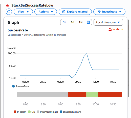
StackSetSuccessRateAlarm:
Type: AWS::CloudWatch::Alarm
Properties:
AlarmDescription: "Alarm when StackSet operation success rate is low"
MetricName: SuccessRate
Namespace: "StackSetMonitoring"
Statistic: Average
Period: 300
EvaluationPeriods: 3
DatapointsToAlarm: 2
Threshold: 80
ComparisonOperator: LessThanThreshold
AlarmActions: [!Ref StackSetAlertsTopic]
Dimensions: [{Name: StackSetName, Value: !Ref StackSetName}]
Outputs:
SNSTopicArn:
Description: The ARN of the SNS topic for alerts
Value: !Ref StackSetAlertsTopic
DashboardURL:
Description: URL to the CloudWatch Dashboard
Value: !Sub https://console.aws.amazon.com/cloudwatch/home?region=${AWS::Region}#dashboards:name=StackSetMonitoring
LambdaLogGroupName:
Description: Name of the CloudWatch Log Group for Lambda logs
Value: !Ref LambdaLogGroup
DeadLetterQueueArn:
Description: ARN of the Dead Letter Queue for Lambda function failures
Value: !GetAtt StackSetMonitorDLQ.Arn
DeadLetterQueueURL:
Description: URL of the Dead Letter Queue for monitoring failed Lambda executions
Value: !Ref StackSetMonitorDLQ
TestLambdaCommand:
Description: Command to manually test the Lambda function
Value: !Sub "aws lambda invoke --function-name ${StackSetMonitorLambda} --payload '{}' response.json && cat response.json"
LambdaFunctionArn:
Description: ARN of the Lambda function configured with VPC
Value: !GetAtt StackSetMonitorLambda.Arn
LambdaSecurityGroupId:
Description: Security Group ID created for the Lambda function
Value: !Ref LambdaSecurityGroup
VpcConfiguration:
Description: VPC configuration summary for the Lambda function
Value: !Sub
- "VPC: ${VpcId}, Subnets: ${SubnetList}, Security Groups: ${LambdaSecurityGroup}"
- SubnetList: !Join [',', !Ref SubnetIds]
You need to run the following CLI command to deploy the CloudFormation stacks. You can change the ParameterValue of StackSetName“your-stackset-name” by the name of the StackSet you want to monitor. The default value is “security-baseline”. Your CLI profile should use region=“us-east-1“.
aws cloudformation create-stack --stack-name stackset-monitor --template-body file://StackSetMonitor.yml --parameters ParameterKey=StackSetName,ParameterValue="security-baseline" --capabilities CAPABILITY_IAM
AWS CLI to deploy the StackSetMonitor.yml CloudFormation template
The CLI output should look like the following:
{"StackId": "arn:aws:cloudformation:...."}
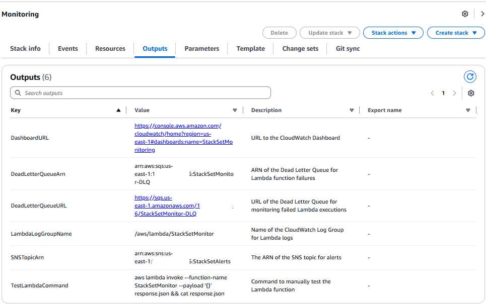
Here’s the expected output for the CloudFormation template:

StackSetMonitor Console output
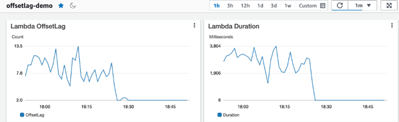
And an example of Amazon CloudWatch Dashboard and Alarm screen:

Amazon CloudWatch Dashboard screenshot for StackSetMonitor stack to track StackSet operations success rate

Amazon CloudWatch Alarm screenshot for StackSetMonitor stack to track StackSet operations success rate
SNS subscription setup involves retrieving the topic ARN from stack outputs and configuring notifications for email or SMS endpoints (below example CLI for email subscription):
aws sns subscribe --topic-arn $SNS_TOPIC_ARN --protocol email --notification-endpoint [email protected]
AWS CLI to subscribe to the topic providing the user email
Cost:
The estimated monthly expenses ranges between 5 and 15 USD depending on StackSet activity levels, with approximately 2,880 Lambda executions per day (each minute) under the default monitoring schedule.
The solution supports customization of monitoring frequency by modifying the ScheduleExpression from the default one-minute interval. The cost will decrease if the monitoring is less frequent.
Cleanup:
For cleanup, you can run the following command lines:
- To cleanup the Stack Instances and StackSets created in the Core Deployment Strategies section:
aws cloudformation delete-stack-instances --stack-set-name security-baseline --deployment-targets OrganizationalUnitIds=ou-xxx --regions us-east-1 eu-west-1 --region us-east-1 --no-retain-stack
AWS CLI to delete the Stack Instances
You need to change the parameter OrganizationalUnitIds value with the name of the OU, the parameter regions with the list of regions where you want to delete your stack instances, and the value of the stack-set-name parameter (security-baseline, monitoring-baseline, balanced-deployment…).
Then you can delete the StackSet:
aws cloudformation delete-stack-set --stack-set-name security-baseline
AWS CLI to delete the StackSet
You can change the value of the stack-set-name parameter.
- To cleanup the stackset-monitor stack
aws cloudformation delete-stack --stack-name stackset-monitor
AWS CLI to delete the stackset-monitor Stack
You can also remove any IAM roles/policies that you specifically created for this blog that you might not need anymore
Conclusion
Throughout this guide, we’ve explored the nuanced approaches to AWS CloudFormation StackSets deployments across large-scale environments. The key takeaways include:
- Balance is Critical: Every deployment strategy requires careful consideration of the trade-offs between speed, safety, and scale based on your organizational needs.
- Progressive Adoption Works: For most organizations, a progressive deployment approach with validation gates provides the optimal balance of safety and efficiency.
- Organizational Context Matters: Enterprise, startup, and regulated industry patterns demonstrate that deployment strategies should be tailored to your specific business requirements and risk tolerance.
- Monitoring is Essential: As organizations scale to hundreds of accounts, comprehensive monitoring becomes critical for maintaining visibility and ensuring compliance.
These different approaches will help you adopt the right strategy for your AWS CloudFormation Stacksets deployments in your AWS Organization.
You can now test these different approaches on your sandbox environment, before adapting them for your specific needs, in order to balance Speed, Safety and Scale to optimize your deployments.

![Screenshot of AI-DLC workspace detection phase showing the Amazon Q chat interface. The left sidebar displays the file tree with an 'aidlc-doc' folder highlighted. The main chat area shows the Inception Phase - Workspace Detection stage with explanatory text about analyzing the workspace. Five callout annotations explain: 1) Workflow creates aidlc-doc directory for storing AI-DLC generated artifacts; 2) The workflow tracks its progress in aidlc-metadata.json for error recovery and session continuity; 3) The audit.md file stores user's prompts; 4) Workflow highlights the AI-DLC phase and stage name with a clear heading for easy tracking; 5) Workflow loads detailed stage-level behavior files dynamically such that they don't consume the context window statically. At the bottom, a user approval prompt shows 'mkdir -p /Users/[...]/NewConsumerPortal/aidlc-docs' with the user asked to approve the 'mkdir' command.](https://d2908q01vomqb2.cloudfront.net/7719a1c782a1ba91c031a682a0a2f8658209adbf/2025/11/24/04_AI-DLC_workspace_detection-1.png)


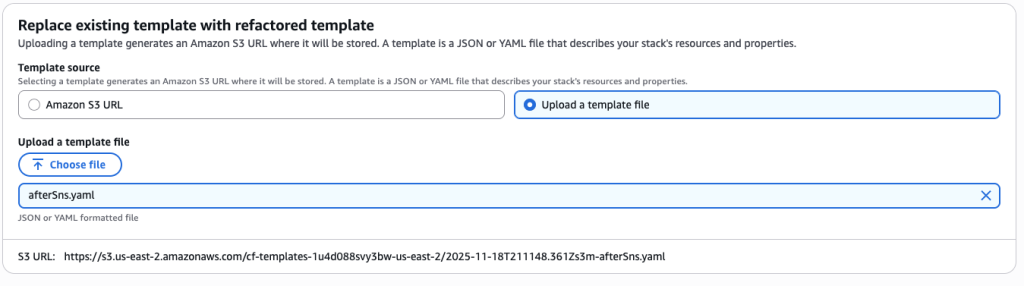
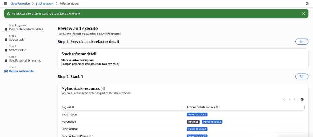
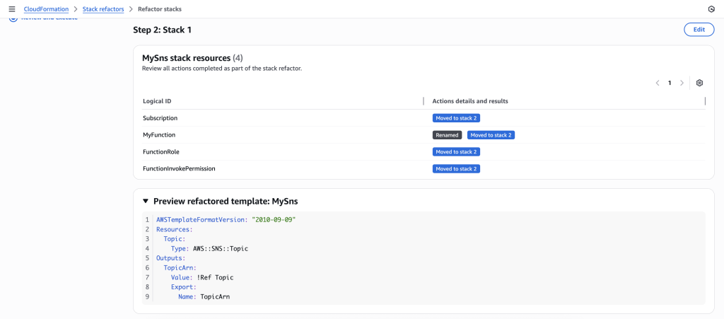
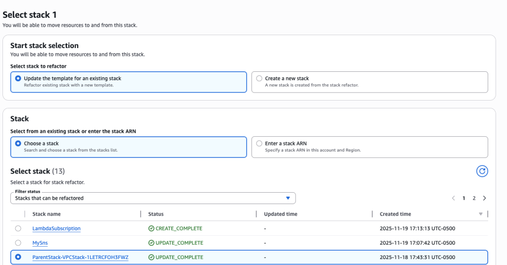
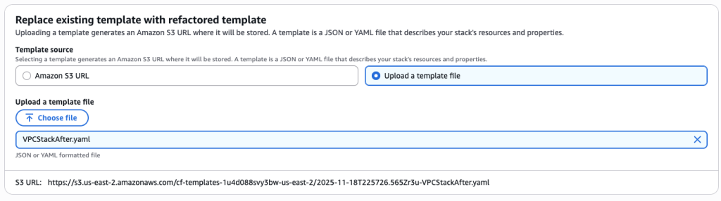
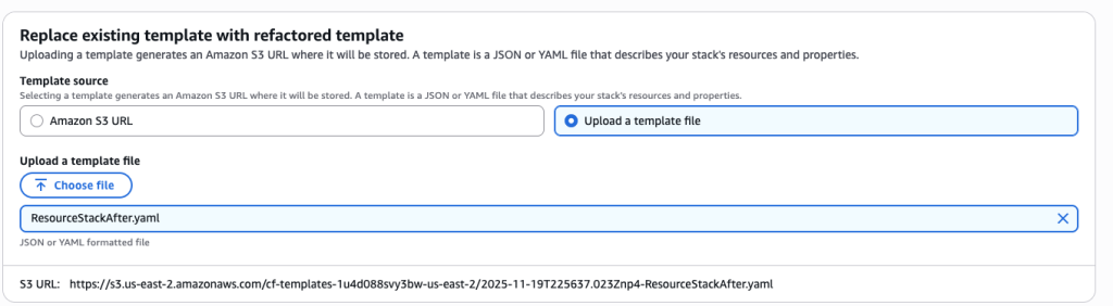
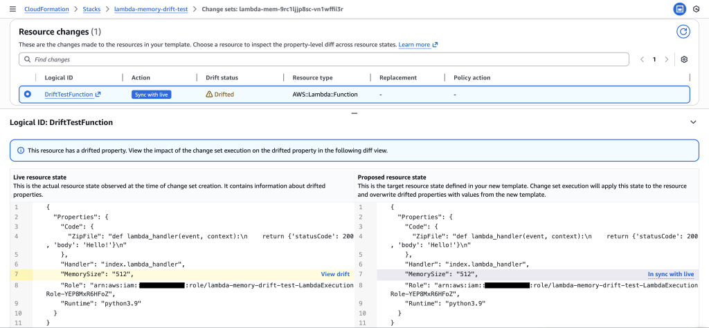
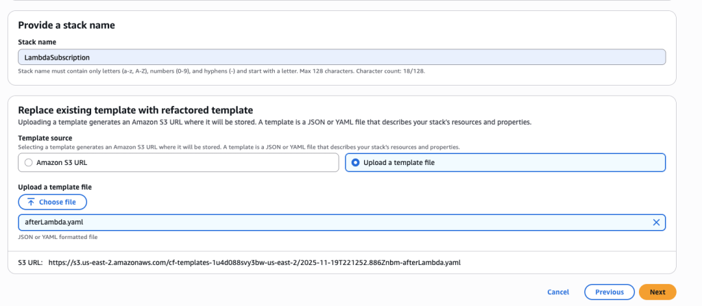 In some scenarios, CloudFormation console can automatically detect logical resource ID renames and pre-fill the mapping for you. The resource mapping is required when there are logical resource ID changes between the original stack and refactored template. Ensure that the mappings are correct before proceeding to the next step.