Post Syndicated from Mohammad Sabeel original https://aws.amazon.com/blogs/big-data/build-an-analytics-pipeline-that-is-resilient-to-avro-schema-changes-using-amazon-athena/
As technology progresses, the Internet of Things (IoT) expands to encompass more and more things. As a result, organizations collect vast amounts of data from diverse sensor devices monitoring everything from industrial equipment to smart buildings. These sensor devices frequently undergo firmware updates, software modifications, or configuration changes that introduce new monitoring capabilities or retire obsolete metrics. As a result, the data structure (schema) of the information transmitted by these devices evolves continuously.
Organizations commonly choose Apache Avro as their data serialization format for IoT data due to its compact binary format, built-in schema evolution support, and compatibility with big data processing frameworks. This becomes crucial when sensor manufacturers release updates that add new metrics or deprecate old ones, allowing for seamless data processing. For example, when a sensor manufacturer releases a firmware update that adds new temperature precision metrics or deprecates legacy vibration measurements, Avro’s schema evolution capabilities allow for seamless handling of these changes without breaking existing data processing pipelines.
However, managing schema evolution at scale presents significant challenges. For example, organizations need to store and process data from thousands of sensors and update their schemas independently, handle schema changes occurring as frequently as every hour due to rolling device updates, maintain historical data compatibility while accommodating new schema versions, query data across multiple time periods with different schemas for temporal analysis, and ensure minimal query failures due to schema mismatches.
To address this challenge, this post demonstrates how to build such a solution by combining Amazon Simple Storage Service (Amazon S3) for data storage, AWS Glue Data Catalog for schema management, and Amazon Athena for one-time querying. We’ll focus specifically on handling Avro-formatted data in partitioned S3 buckets, where schemas can change frequently while providing consistent query capabilities across all data regardless of schema versions.
This solution is specifically designed for Hive-based tables, such as those in the AWS Glue Data Catalog, and is not applicable for Iceberg tables. By implementing this approach, organizations can build a highly adaptive and resilient analytics pipeline capable of handling extremely frequent Avro schema changes in partitioned S3 environments.
Solution overview
In this post as an example, we’re simulating a real-world IoT data pipeline with the following requirements:
- IoT devices continuously upload sensor data in Avro format to an S3 bucket, simulating real-time IoT data ingestion
- The schema change happens frequently over time
- Data will be partitioned hourly to reflect typical IoT data ingestion patterns
- Data needs to be queryable using the most recent schema version through Amazon Athena.
To achieve these requirements, we demonstrate the solution using automated schema detection. We use AWS Command Line Interface (AWS CLI) and AWS SDK for Python (Boto3) scripts to simulate an automated mechanism that continually monitors the S3 bucket for new data, detects schema changes in incoming Avro files, and triggers necessary updates to the AWS Glue Data Catalog.
For schema evolution handling, our solution will demonstrate how to create and update table definitions in the AWS Glue Data Catalog, incorporate Avro schema literals to handle schema changes, and use the Athena partition projection for efficient querying across schema versions. The data steward or admin needs to know when and how the schema is updated so that the admin can manually change the columns in the UpdateTable API call. For validation and querying, we use Amazon Athena queries to verify table definitions and partition details and demonstrate successful querying of data across different schema versions. By simulating these components, our solution addresses the key requirements outlined in the introduction:
- Handling frequent schema changes (as often as hourly)
- Managing data from thousands of sensors updating independently
- Maintaining historical data compatibility while accommodating new schemas
- Enabling querying across multiple time periods with different schemas
- Minimizing query failures due to schema mismatches
Although in a production environment this would be integrated into a sophisticated IoT data processing application, our simulation using AWS CLI and Boto3 scripts effectively demonstrates the principles and techniques for managing schema evolution in large-scale IoT deployments.
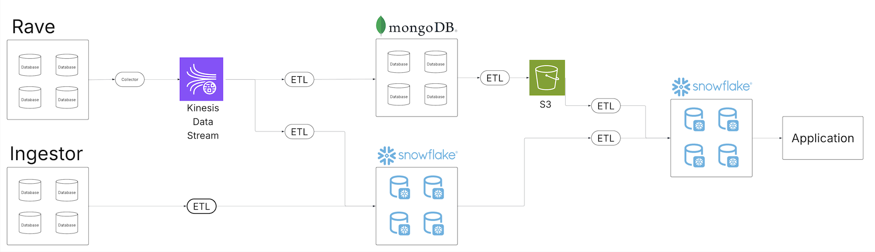
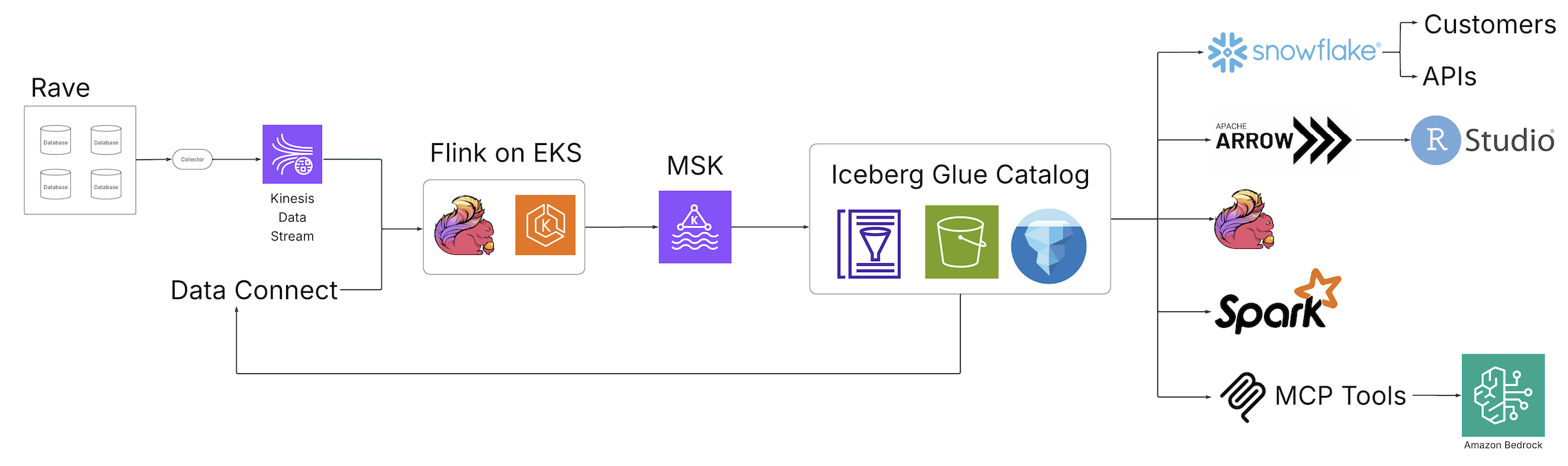
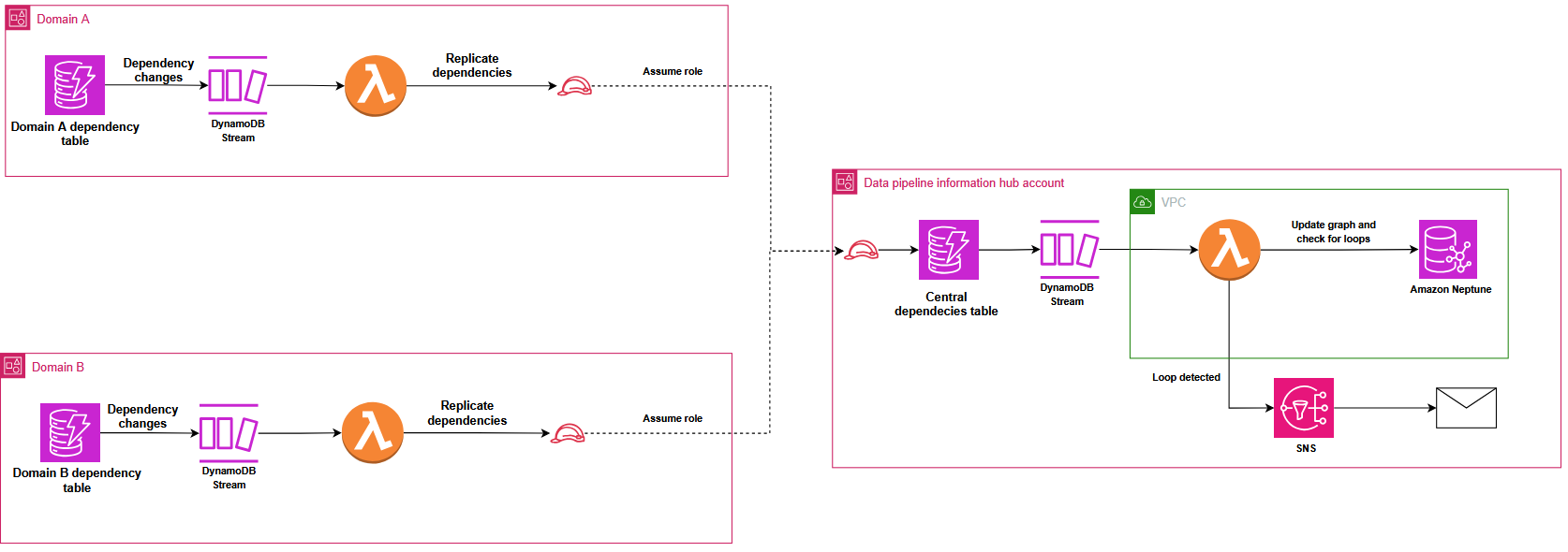
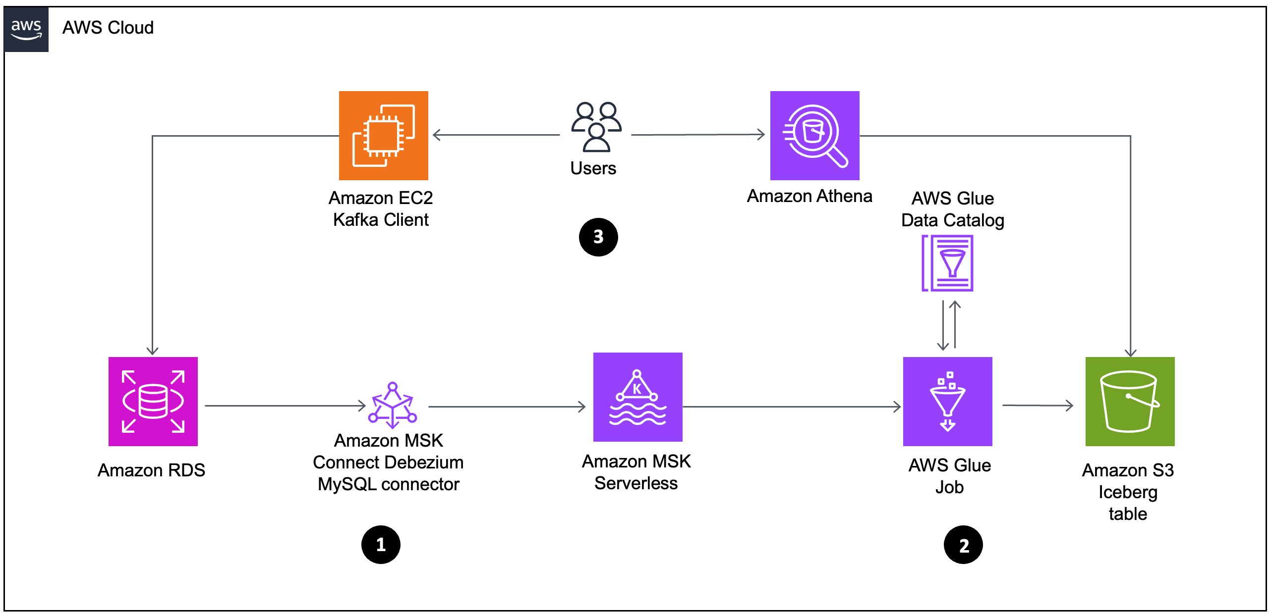
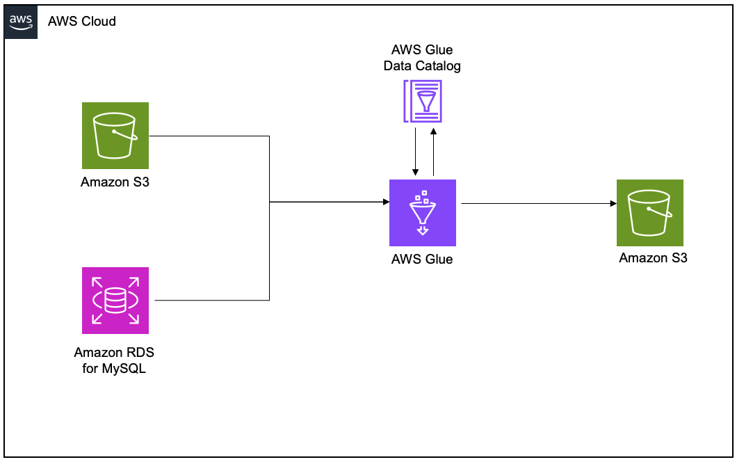
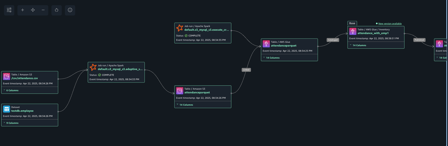
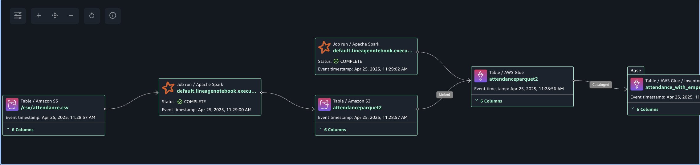
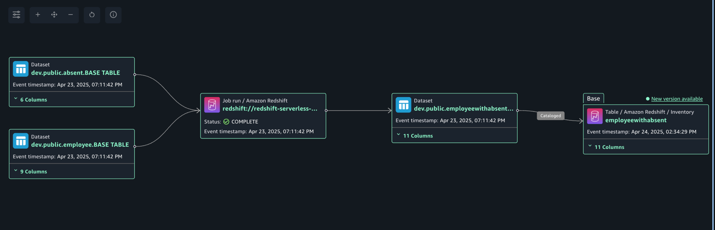
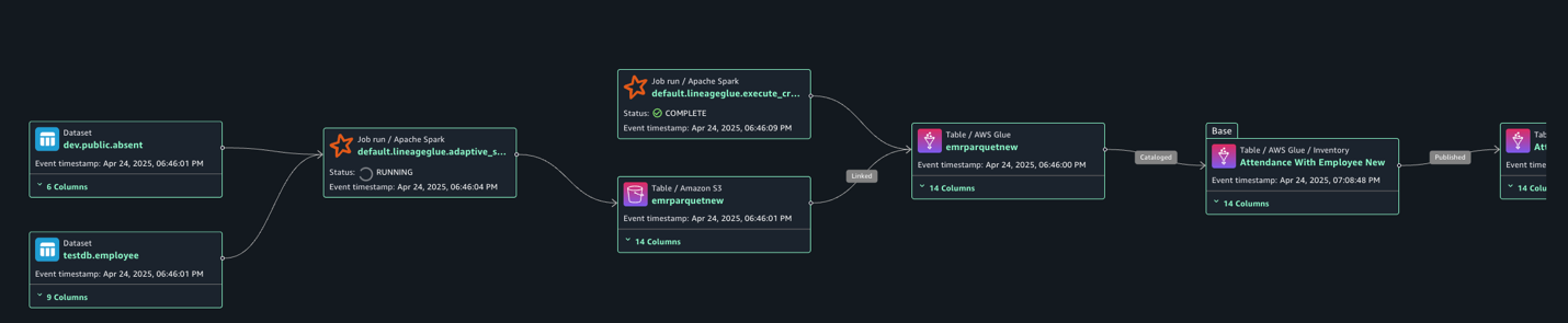
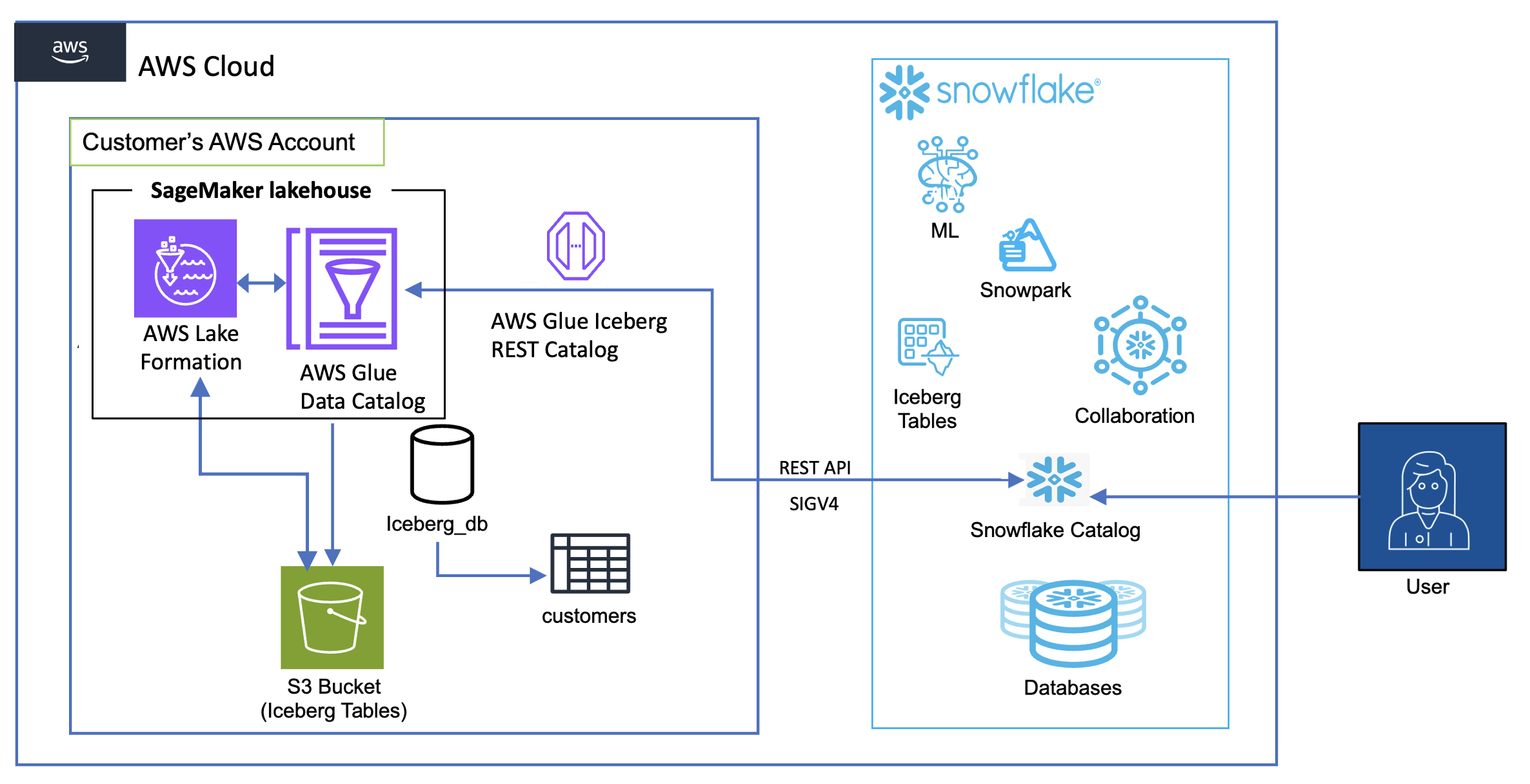
The following diagram illustrates the solution architecture.

Prerequisites:
To perform the solution, you need to have the following prerequisites:
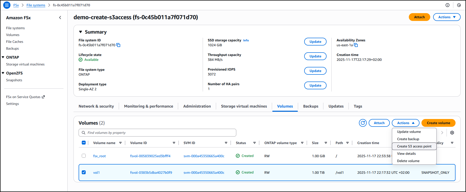
Create the base table
In this section, we simulate the initial setup of a data pipeline for IoT sensor data. This step is crucial because it establishes the foundation for our schema evolution demonstration. This initial table serves as the starting point from which our schema will evolve. It allows us to demonstrate how to handle schema changes over time. In this scenario, the base table contains three key fields: customerID (bigint), sentiment (a struct containing customerrating), and dt (string) as a partition column. And Avro schema literal (‘avro.schema.literal’)along with other configurations. Follow these steps:
- Create a new file named
`CreateTableAPI.py` with the following content. Replace 'Location': 's3://amzn-s3-demo-bucket/' with your S3 bucket details and <AWS Account ID> with your AWS account ID:
import boto3
import time

if __name__ == '__main__':
    database_name = " blogpostdatabase"
    table_name = "blogpost_table_test"
    catalog_id = ''
    client = boto3.client('glue')

    response = client.create_table(
        CatalogId=catalog_id,
        DatabaseName=database_name,
        TableInput={
            'Name': table_name,
            'Description': 'sampletable',
            'Owner': 'root',
            'TableType': 'EXTERNAL_TABLE',
            'LastAccessTime': int(time.time()),
            'LastAnalyzedTime': int(time.time()),
            'Retention': 0,
            'Parameters' : {
                'avro.schema.literal': '{"type" : "record", "name" : "customerdata", "namespace" : "com.data.test.avro", "fields" : [{ "name" : "customerID", "type" : "long", "default" : -1 },{ "name" : "sentiment", "type" : [ "null", { "type" : "record", "name" : "sentiment", "doc" : "***** CoreETL ******", "fields" : [ { "name" : "customerrating", "type" : "long", "default" : 0 }] } ], "default" : 0 }]}'
            },
            'StorageDescriptor': {
                'Columns': [
                    {
                        'Name': 'customerID',
                        'Type': 'bigint',
                        'Comment': 'from deserializer'
                    },
                    {
                        'Name': 'sentiment',
                        'Type': 'struct<customerrating:bigint>',
                        'Comment': 'from deserializer'
                    }
                ],
                'Location': 's3:///',
                'InputFormat': 'org.apache.hadoop.hive.ql.io.avro.AvroContainerInputFormat',
                'OutputFormat': 'org.apache.hadoop.hive.ql.io.avro.AvroContainerOutputFormat',
                'SerdeInfo': {
                    'SerializationLibrary': 'org.apache.hadoop.hive.serde2.avro.AvroSerDe',
                    'Parameters': {
                        'avro.schema.literal': '{"type" : "record", "name" : "customerdata", "namespace" : "com.data.test.avro", "fields" : [{ "name" : "customerID", "type" : "long", "default" : -1 },{ "name" : "sentiment", "type" : [ "null", { "type" : "record", "name" : "sentiment", "doc" : "***** CoreETL ******", "fields" : [ { "name" : "customerrating", "type" : "long", "default" : 0 } ] } ], "default" : 0 }]}'
                    }
                }
            },
            'PartitionKeys': [
                {
                    'Name': 'dt',
                    'Type': 'string'
                }
            ]
        }
    )

    print(response)
- Run the script using the command:
python3 CreateTableAPI.py
The schema literal serves as a form of metadata, providing a clear description of your data structure. In Amazon Athena, Avro table schema Serializer/Deserializer (SerDe) properties are essential for schema is compatible with the data stored in files, facilitating accurate translation for query engines. These properties enable the precise interpretation of Avro-formatted data, allowing query engines to correctly read and process the information during execution.
The Avro schema literal provides a detailed description of the data structure at the partition level. It defines the fields, their data types, and any nested structures within the Avro data. Amazon Athena uses this schema to correctly interpret the Avro data stored in Amazon S3. It makes sure that each field in the Avro file is mapped to the correct column in the Athena table.
The schema information helps Athena optimize query run by understanding the data structure in advance. It can make informed decisions about how to process and retrieve data efficiently. When the Avro schema changes (for example, when new fields are added), updating the schema literal allows Athena to recognize and work with the new structure. This is crucial for maintaining query compatibility as your data evolves over time. The schema literal provides explicit type information, which is essential for Avro’s type system. This provides accurate data type conversion between Avro and Athena SQL types.
For complex Avro schemas with nested structures, the schema literal informs Athena how to navigate and query these nested elements. The Avro schema can specify default values for fields, which Athena can use when querying data where certain fields might be missing. Athena can use the schema to perform compatibility checks between the table definition and the actual data, helping to identify potential issues. In the SerDe properties, the schema literal tells the Avro SerDe how to deserialize the data when reading it from Amazon S3.
It’s crucial for the SerDe to correctly interpret the binary Avro format into a form Athena can query. The detailed schema information aids in query planning, allowing Athena to make informed decisions about how to execute queries efficiently. The Avro schema literal specified in the table’s SerDe properties provides Athena with the exact field mappings, data types, and physical structure of the Avro file. This enables Athena to perform column pruning by calculating precise byte offsets for required fields, reading only those specific portions of the Avro file from S3 rather than retrieving the entire record.
Parameters' : {
                'avro.schema.literal': '{"type" : "record", "name" : "customerdata", "namespace" : "com.data.test.avro", "fields" : [{ "name" : "customerID", "type" : "long", "default" : -1 },{ "name" : "sentiment", "type" : [ "null", { "type" : "record", "name" : "sentiment", "doc" : "***** CoreETL ******", "fields" : [ { "name" : "customerrating", "type" : "long", "default" : 0 }] } ], "default" : 0 }]}'
            },
- After creating the table, verify its structure using the
SHOW CREATE TABLE command in Athena:
CREATE EXTERNAL TABLE `blogpost_table_test`(
  `customerid` bigint COMMENT 'from deserializer',
  `sentiment` struct<customerrating:bigint> COMMENT 'from deserializer')
PARTITIONED BY (
  `dt` string)
ROW FORMAT SERDE
  'org.apache.hadoop.hive.serde2.avro.AvroSerDe'
WITH SERDEPROPERTIES (
  'avro.schema.literal'='{\"type\" : \"record\", \"name\" : \"customerdata\", \"namespace\" : \"com.data.test.avro\", \"fields\" : [{ \"name\" : \"customerID\", \"type\" : \"long\", \"default\" : -1 },{ \"name\" : \"sentiment\", \"type\" : [ \"null\", { \"type\" : \"record\", \"name\" : \"sentiment\", \"doc\" : \"***** CoreETL ******\", \"fields\" : [ { \"name\" : \"customerrating\", \"type\" : \"long\", \"default\" : 0 } ] } ], \"default\" : 0 }]}')
STORED AS INPUTFORMAT
  'org.apache.hadoop.hive.ql.io.avro.AvroContainerInputFormat'
OUTPUTFORMAT
  'org.apache.hadoop.hive.ql.io.avro.AvroContainerOutputFormat'
LOCATION
  's3://amzn-s3-demo-bucket/'
TBLPROPERTIES (
  'avro.schema.literal'='{\"type\" : \"record\", \"name\" : \"customerdata\", \"namespace\" : \"com.data.test.avro\", \"fields\" : [{ \"name\" : \"customerID\", \"type\" : \"long\", \"default\" : -1 },{ \"name\" : \"sentiment\", \"type\" : [ \"null\", { \"type\" : \"record\", \"name\" : \"sentiment\", \"doc\" : \"***** CoreETL ******\", \"fields\" : [ { \"name\" : \"customerrating\", \"type\" : \"long\", \"default\" : 0 } ] } ], \"default\" : 0 }]}')
Note that the table is created with the initial schema as described below:
[
  {
    "Name": "customerid",
    "Type": "bigint",
    "Comment": "from deserializer"
  },
  {
    "Name": "sentiment",
    "Type": "struct<confirmedImpressions:bigint>",
    "Comment": "from deserializer"
  },
  {
    "Name": "dt",
    "Type": "string",
    "PartitionKey": "Partition (0)"
  }
]
With the table structure in place, you can load the first set of IoT sensor data and establish the initial partition. This step is crucial for setting up the data pipeline that will handle incoming sensor data.
- Download the example sensor data from the following S3 bucket
s3://aws-blogs-artifacts-public/artifacts/BDB-4745
Download initial schema from the first partition
aws s3 cp s3://aws-blogs-artifacts-public/artifacts/BDB-4745/dt=2024-03-21/initial_schema_sample1.avro
Download second schema from the second partition
aws s3 cp s3://aws-blogs-artifacts-public/artifacts/BDB-4745/dt=2024-03-22/second_schema_sample2.avro
Download third schema from the third partition
aws s3 cp s3://aws-blogs-artifacts-public/artifacts/BDB-4745/dt=2024-03-23/third_scehama_sample3avro
- Upload the Avro-formatted sensor data to your partitioned S3 location. This represents your first day of sensor readings, organized in the date-based partition structure. Replace the bucket name
amzn-s3-demo-bucket with your S3 bucket name and add a partitioned folder for the dt field.
s3://amzn-s3-demo-bucket/dt=2024-03-21/
- Register this partition in the AWS Glue Data Catalog to make it discoverable. This tells AWS Glue where to find your sensor data for this specific date:
ALTER TABLE iot_sensor_data ADD PARTITION (dt='2024-03-21');
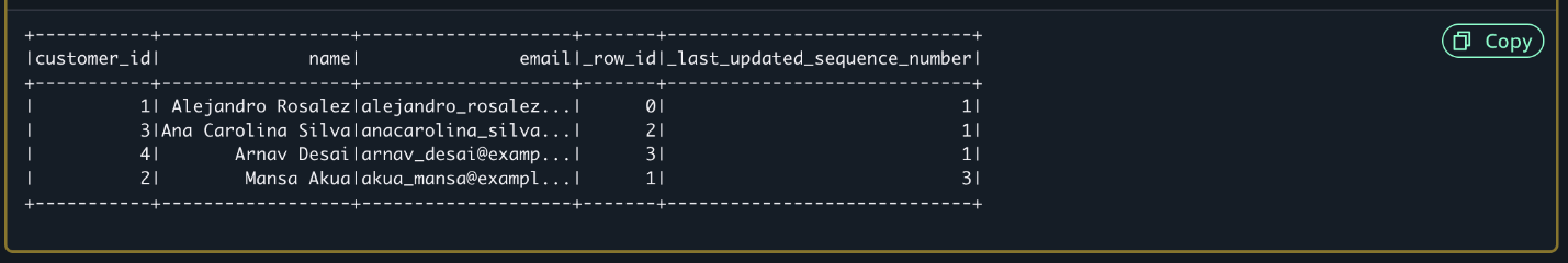
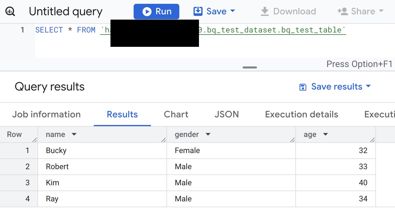
- Validate your sensor data ingestion by querying the newly loaded partition. This query helps verify that your sensor readings are correctly loaded and accessible:
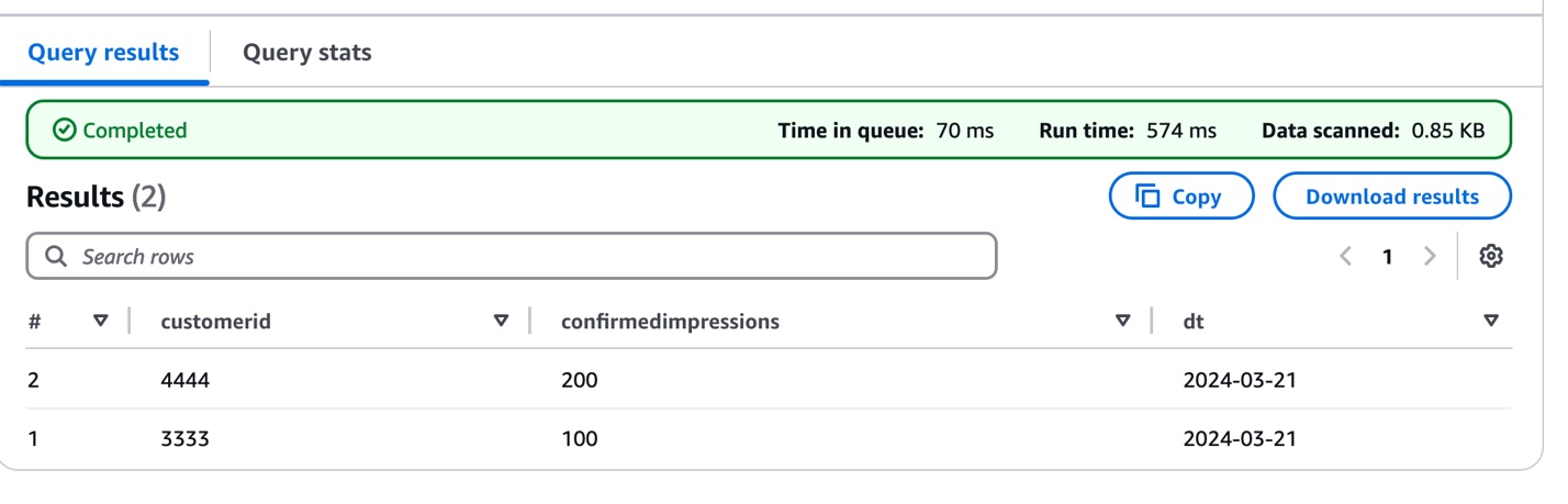
SELECT * FROM "blogpostdatabase "."iot_sensor_data" WHERE dt='2024-03-21';
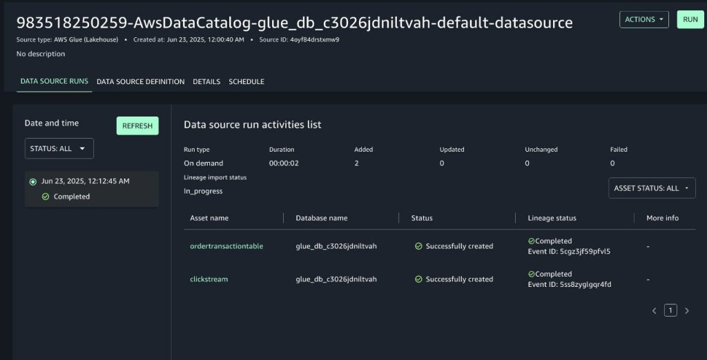
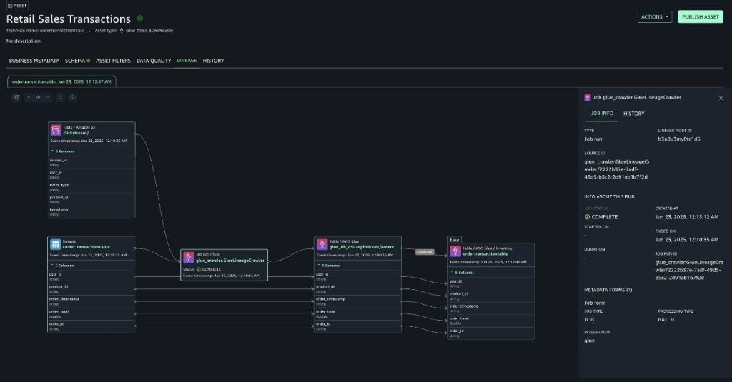
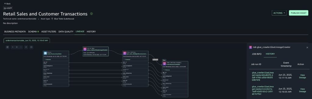
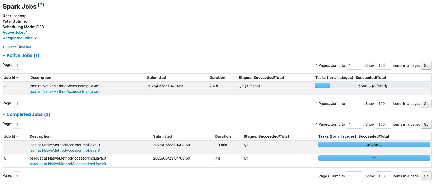
The following screenshot shows the query results.

This initial data load establishes the foundation for the IoT data pipeline, which means you can begin tracking sensor measurements while preparing for future schema evolution as sensor capabilities expand or change.
Now, we demonstrate how the IoT data pipeline handles evolving sensor capabilities by introducing a schema change in the second data batch. As sensors receive firmware updates or new monitoring features, their data structure needs to adapt accordingly. To show this evolution, we add data from sensors that now include visibility measurements:
- Examine the evolved schema structure that accommodates the new sensor capability:
{
  "fields": [
    {
      "Name": "customerid",
      "Type": "bigint",
      "Comment": "from deserializer"
    },
    {
      "Name": "sentiment",
      "Type": "struct<confirmedImpressions:bigint,visibility:bigint>",
      "Comment": "from deserializer"
    },
    {
      "Name": "dt",
      "Type": "string",
      "PartitionKey": "Partition (0)"
    }
  ]
}
Note the addition of the visibility field within the sentiment structure, representing the sensor’s enhanced monitoring capability.
- Upload this enhanced sensor data to a new date partition:
s3://amzn-s3-demo-bucket/dt=2024-03-22/
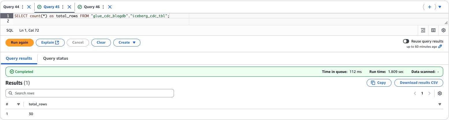
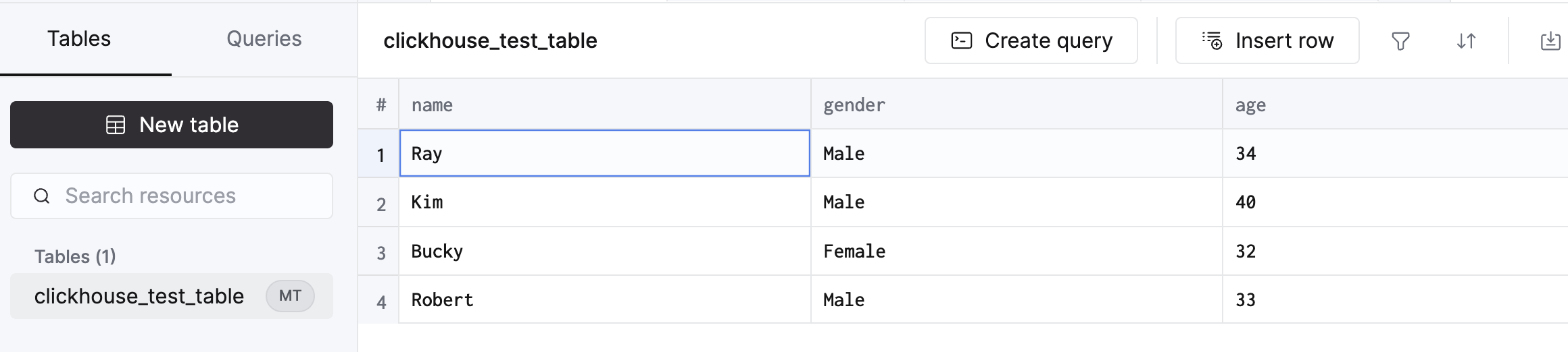
- Verify data consistency across both the original and enhanced sensor readings:
SELECT * FROM "blogpostdatabase"."blogpost_table_test" LIMIT 10;
This demonstrates how the pipeline can handle sensor upgrades while maintaining compatibility with historical data. In the next section, we explore how to update the table definition to properly manage this schema evolution, providing seamless querying across all sensor data regardless of when the sensors were upgraded. This approach is particularly valuable in IoT environments where sensor capabilities frequently evolve, which means you can maintain historical data while accommodating new monitoring features.
Update the AWS Glue table
To accommodate evolving sensor capabilities, you need to update the AWS Glue table schema. Although traditional methods such as MSCK REPAIR TABLE or ALTER TABLE ADD PARTITION work for small datasets for updating partition information, you can use an alternate method to handle tables with more than 100K partitions efficiently.
We use the Athena partition projection, which eliminates the need to process extensive partition metadata, which can be time-consuming for large datasets. Instead, it dynamically infers partition existence and location, allowing for more efficient data management. This method also speeds up query planning by quickly identifying relevant partitions, leading to faster query execution. Additionally, it reduces the number of API calls to the metadata store, potentially lowering costs associated with these operations. Perhaps most importantly, this solution maintains performance as the number of partitions grows, prodicing scalability for evolving datasets. These benefits combine to create a more efficient and cost-effective way of handling schema evolution in large-scale data environments.
To update your table schema to handle the new sensor data, follow these steps:
- Copy the following code into the
UpdateTableAPI.py file:
import boto3

client = boto3.client('glue')

db = 'blogpostdatabase'
tb = 'blogpost_table_test'

response = client.get_table(
    DatabaseName=db,
    Name=tb
)

print(response)


table_input = {
    'Description': response['Table'].get('Description', ''),
    'Name': response['Table'].get('Name', ''),
    'Owner': response['Table'].get('Owner', ''),
    'Parameters': response['Table'].get('Parameters', {}),
    'PartitionKeys': response['Table'].get('PartitionKeys', []),
    'Retention': response['Table'].get('Retention'),
    'StorageDescriptor': response['Table'].get('StorageDescriptor', {}),
    'TableType': response['Table'].get('TableType', ''),
    'ViewExpandedText': response['Table'].get('ViewExpandedText', ''),
    'ViewOriginalText': response['Table'].get('ViewOriginalText', '')

}

for col in table_input['StorageDescriptor']['Columns']:
    if col['Name'] == 'sentiment':
        col['Type'] = 'struct<confirmedImpressions:bigint,visibility:bigint>'


table_input['StorageDescriptor']['SerdeInfo']['Parameters']['avro.schema.literal'] = '{"type" : "record", "name" : "customerdata", "namespace" : "com.data.test.avro", "fields" : [{ "name" : "customerID", "type" : "long", "default" : -1 },{ "name" : "sentiment", "type" : [ "null", { "type" : "record", "name" : "sentiment", "doc" : "***** CoreETL ******", "fields" : [ { "name" : "customerrating", "type" : "long", "default" : 0 },{"name":"visibility","type":"long","default":0}] } ], "default" : 0 }]}'
table_input['Parameters']['avro.schema.literal'] = '{"type" : "record", "name" : "customerdata", "namespace" : "com.data.test.avro", "fields" : [{ "name" : "customerID", "type" : "long", "default" : -1 },{ "name" : "sentiment", "type" : [ "null", { "type" : "record", "name" : "sentiment", "doc" : "***** CoreETL ******", "fields" : [ { "name" : "customerrating", "type" : "long", "default" : 0 },{"name":"visibility","type":"long","default":0} ] } ], "default" : 0 }]}'
table_input['Parameters']['projection.dt.type'] = 'date'
table_input['Parameters']['projection.dt.format'] = 'yyyy-MM-dd'
table_input['Parameters']['projection.enabled'] = 'true'
table_input['Parameters']['projection.dt.range'] = '2024-03-21,NOW'

response = client.update_table(
    DatabaseName=db,
    TableInput=table_input
)
This Python script demonstrates how to update an AWS Glue table to accommodate schema evolution and enable partition projection:
- It uses Boto3 to interact with AWS Glue API.
- Retrieves the current table definition from the AWS Glue Data Catalog.
- Updates the
'sentiment' column structure to include new fields.
- Modifies the Avro schema literal to reflect the updated structure.
- Adds partition projection parameters for the partition column
dt
table_input['Parameters']['projection.dt.type'] = 'date'
table_input['Parameters']['projection.dt.format'] = 'yyyy-MM-dd'
table_input['Parameters']['projection.enabled'] = 'true'
table_input['Parameters']['projection.dt.range'] = '2024-03-21,NOW'
- Sets projection type to
'date'
- Defines date format as
'yyyy-MM-dd'
- Enables partition projection
- Sets date range from
'2024-03-21' to 'NOW'
projection.date.type='date' --> Data type of the partition column
projection.date.format='yyyy-MM-dd' -> Data format of the partition column
projection.enabled='true' -> Enable the partition projection
projection.date.range='2024-04-26,NOW'. -> The range of the partition column
- Run the script using the following command:
python3 UpdateTableAPI.py
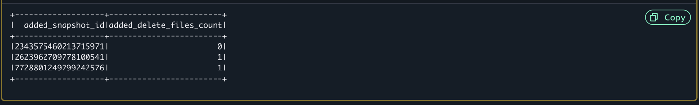
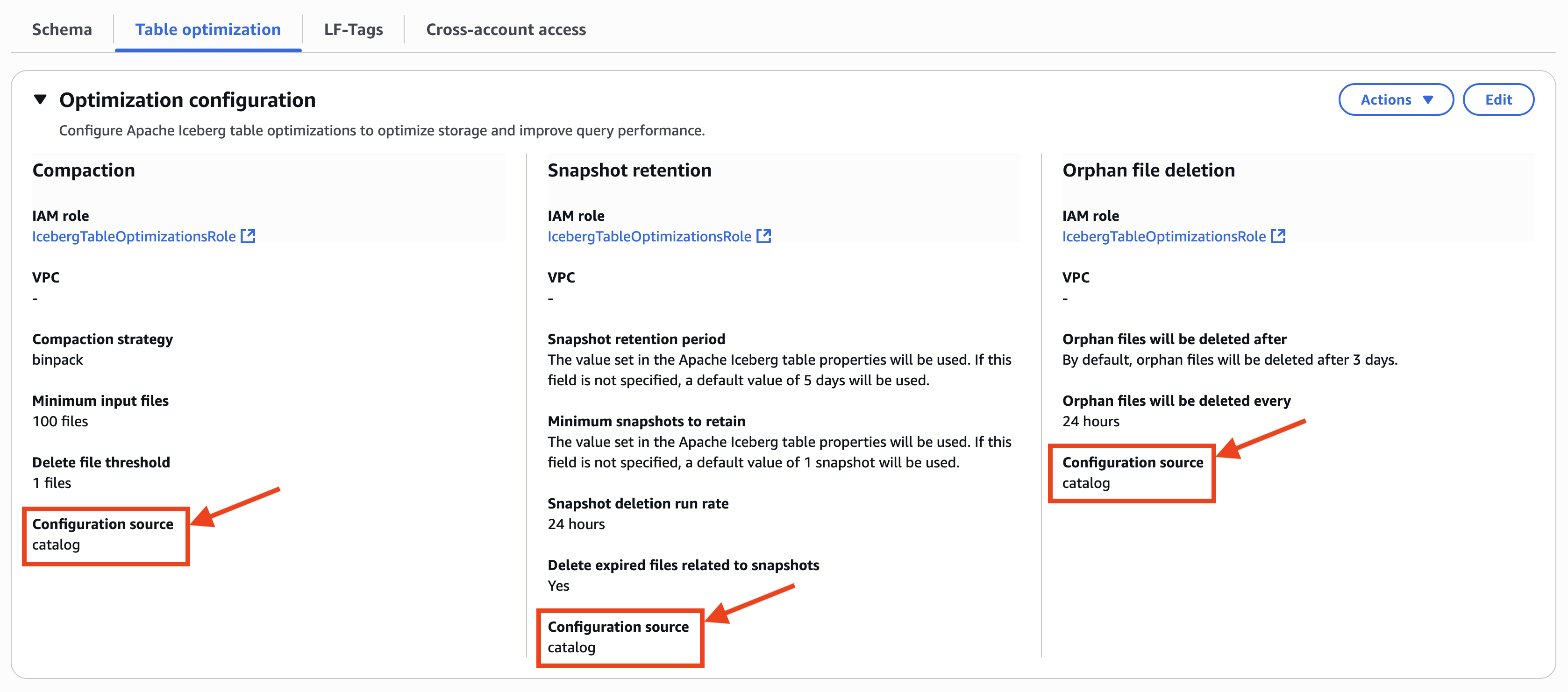
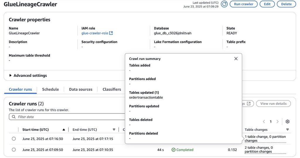
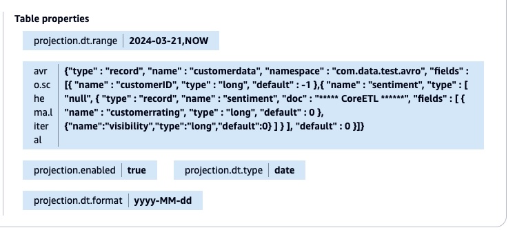
The script applies all changes back to the AWS Glue table using the UpdateTable API call. The following screenshot shows the table property with the new Avro schema literal and the partition projection.

After the table property is updated, you don’t need to add the partitions manually using the MSCK REPAIR TABLE or ALTER TABLE command. You can validate the result by running the query in the Athena console.
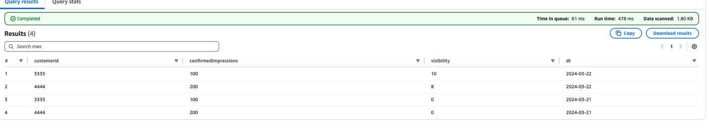
SELECT * FROM "blogpostdatabase"." blogpost_table_test " limit 10;
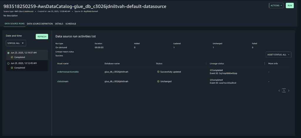
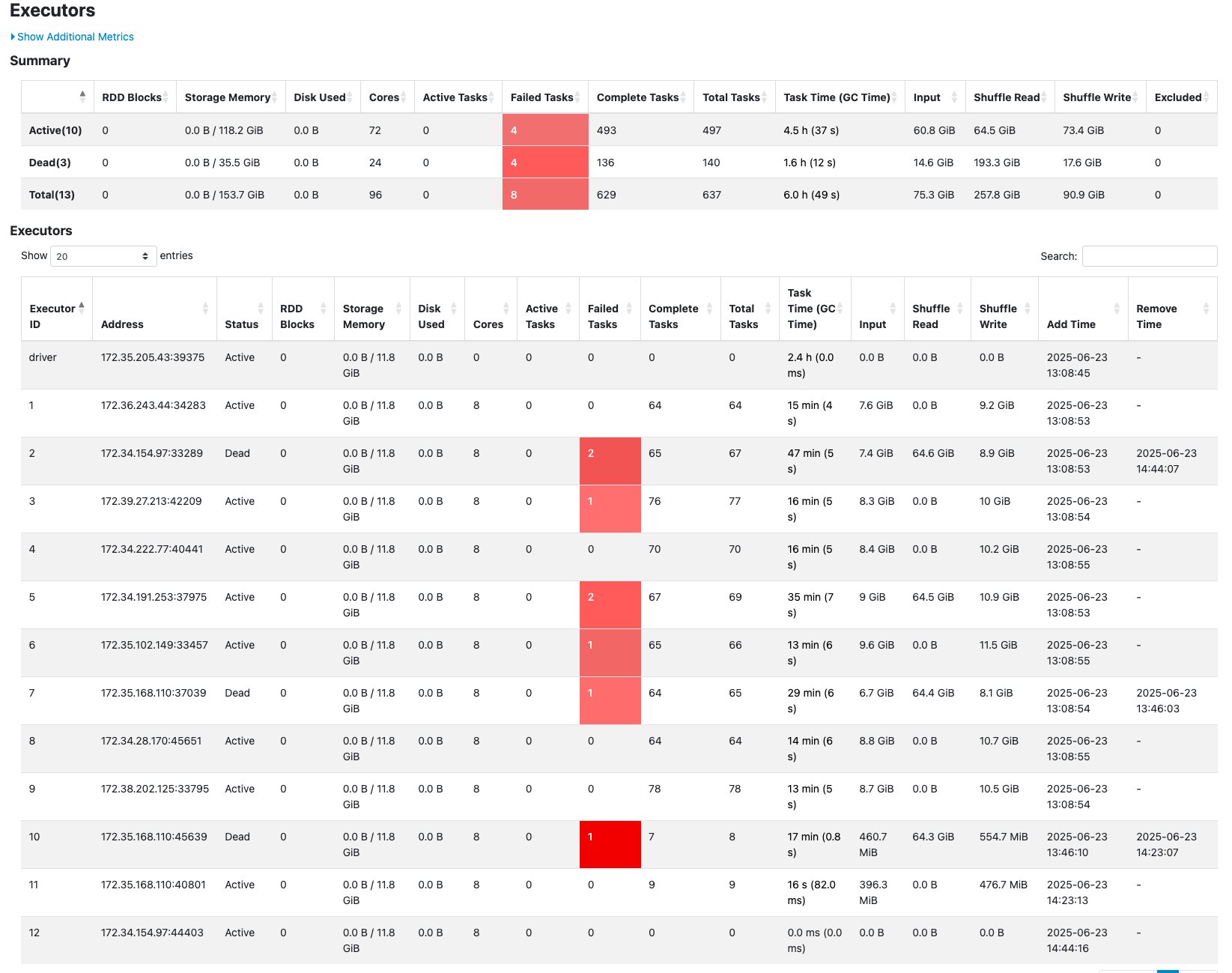
The following screenshot shows the query results.

This schema evolution strategy efficiently handles new data fields across different time periods. Consider the 'visibility' field introduced on 2024-03-22. For data from 2024-03-21, where this field doesn’t exist, the solution automatically returns a default value of 0. This approach makes the query consistent across all partitions, regardless of their schema version.
Here’s the Avro schema configuration that enables this flexibility:
{
  "type": "record",
  "name": "customerdata",
  "fields": [
    {"name": "customerID", "type": "long", "default": -1},
    {"name": "sentiment", "type": ["null", {
      "type": "record",
      "name": "sentiment",
      "fields": [
        {"name": "customerrating", "type": "long", "default": 0},
        {"name": "visibility", "type": "long", "default": 0}
      ]
    }], "default": null}
  ]
}
Using this configuration, you can run queries across all partitions without modifications, maintain backward compatibility without data migration, and support gradual schema evolution without breaking existing queries.
Building on the schema evolution example, we now introduce a third enhancement to the sensor data structure. This new iteration adds a text-based classification capability through a 'category' field (string type) to the sentiment structure. This represents a real-world scenario where sensors receive updates that add new classification capabilities, requiring the data pipeline to handle both numeric measurements and textual categorizations.
The following is the enhanced schema structure:
{
  "fields": [
    {
      "Name": "customerid",
      "Type": "bigint"
    },
    {
      "Name": "sentiment",
      "Type": "struct<confirmedImpressions:bigint,visibility:bigint,category:string>"
    },
    {
      "Name": "dt",
      "Type": "string"
    }
  ]
}
This evolution demonstrates how the solution flexibly accommodates different data types as sensor capabilities expand while maintaining compatibility with historical data.
To implement this latest schema evolution for the new partition (dt=2024-03-23), we update the table definition to include the ‘category’ field. Here’s the modified UpdateTableAPI.py script that handles this change:
- Update the file
UpdateTableAPI.py:
import boto3

client = boto3.client('glue')

db = 'blogpostdatabase'
tb = 'blogpost_table_test'

response = client.get_table(
DatabaseName=db,
Name=tb
)

print(response)


table_input = {
'Description': response['Table'].get('Description', ''),
'Name': response['Table'].get('Name', ''),
'Owner': response['Table'].get('Owner', ''),
'Parameters': response['Table'].get('Parameters', {}),
'PartitionKeys': response['Table'].get('PartitionKeys', []),
'Retention': response['Table'].get('Retention'),
'StorageDescriptor': response['Table'].get('StorageDescriptor', {}),
'TableType': response['Table'].get('TableType', ''),
'ViewExpandedText': response['Table'].get('ViewExpandedText', ''),
'ViewOriginalText': response['Table'].get('ViewOriginalText', '')

}

for col in table_input['StorageDescriptor']['Columns']:
if col['Name'] == 'sentiment':
col['Type'] = 'struct<confirmedImpressions:bigint,visibility:bigint,category:string>'


table_input['StorageDescriptor']['SerdeInfo']['Parameters']['avro.schema.literal'] = '{"type" : "record", "name" : "customerdata", "namespace" : "com.data.test.avro", "fields" : [{ "name" : "customerID", "type" : "long", "default" : -1 },{ "name" : "sentiment", "type" : [ "null", { "type" : "record", "name" : "sentiment", "doc" : "***** CoreETL ******", "fields" : [ { "name" : "customerrating", "type" : "long", "default" : 0 },{"name":"visibility","type":"long","default":0},{"name":"category","type":"string","default":"null"} ] } ], "default" : 0 }]}'
table_input['Parameters']['avro.schema.literal'] = '{"type" : "record", "name" : "customerdata", "namespace" : "com.data.test.avro", "fields" : [{ "name" : "customerID", "type" : "long", "default" : -1 },{ "name" : "sentiment", "type" : [ "null", { "type" : "record", "name" : "sentiment", "doc" : "***** CoreETL ******", "fields" : [ { "name" : "customerrating", "type" : "long", "default" : 0 },{"name":"visibility","type":"long","default":0},{"name":"category","type":"string","default":"null"} ] } ], "default" : 0 }]}'
table_input['Parameters']['projection.dt.type'] = 'date'
table_input['Parameters']['projection.dt.format'] = 'yyyy-MM-dd'
table_input['Parameters']['projection.enabled'] = 'true'
table_input['Parameters']['projection.dt.range'] = '2024-03-21,NOW'

response = client.update_table(
DatabaseName=db,
TableInput=table_input
)
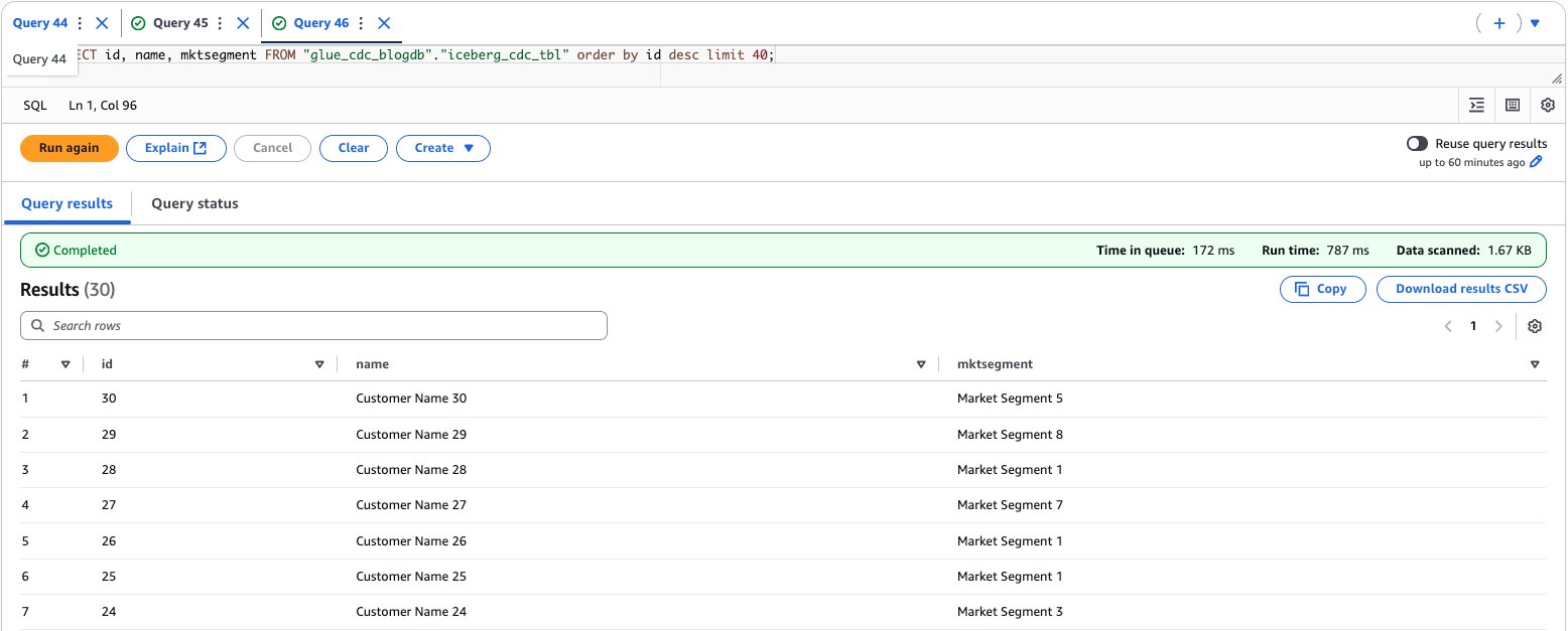
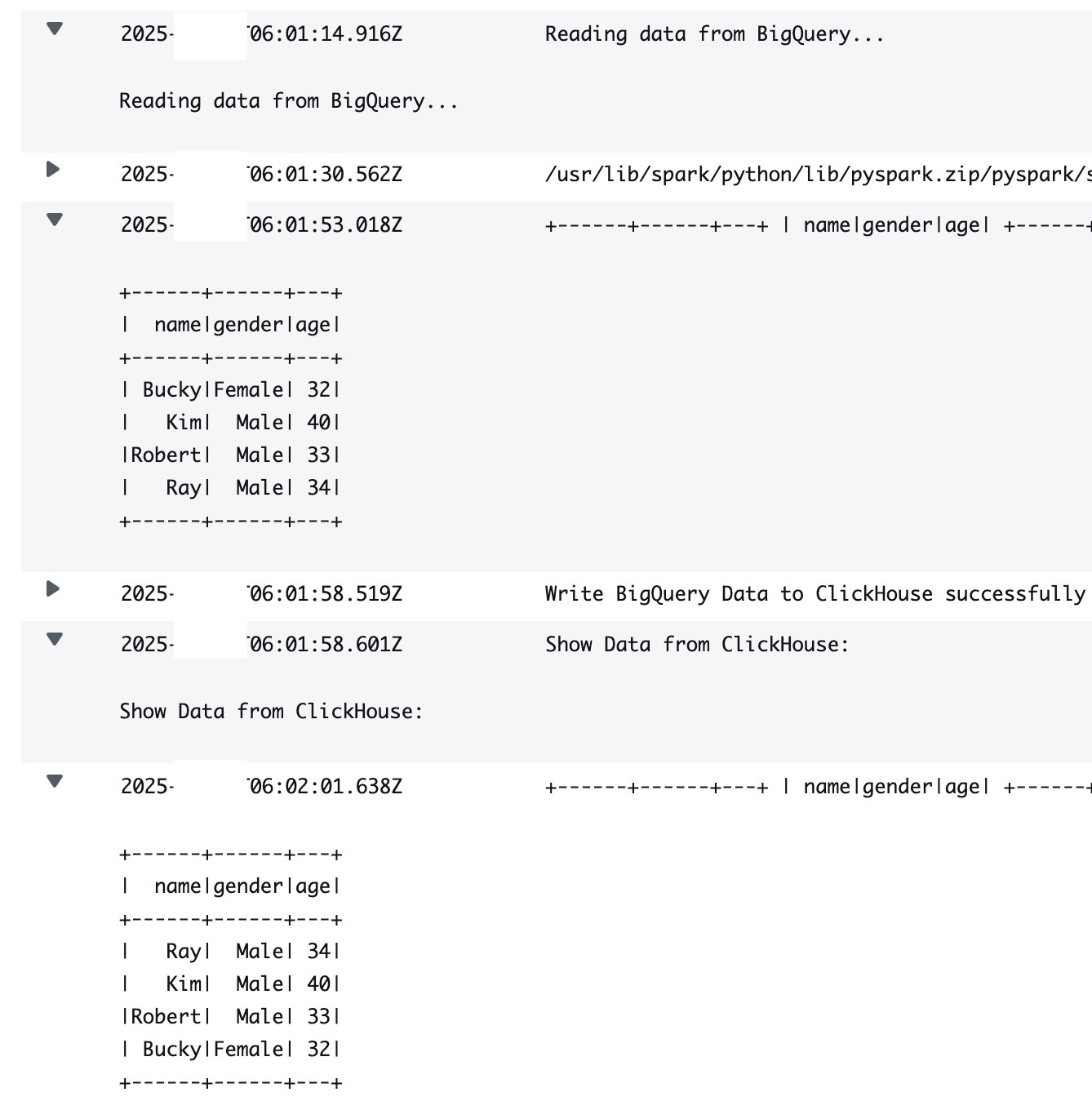
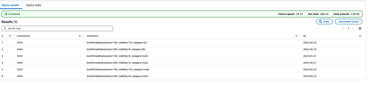
- Verify the changes by running the following query:
SELECT * FROM "blogpostdatabase"."blogpost_table_test" LIMIT 10;
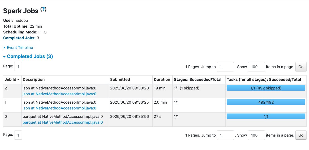
The following screenshot shows the query results.

There are three key changes in this update:
- Added
'category' field (string type) to the sentiment structure
- Set default value
"null" for the category field
- Maintained existing partition projection settings
To support that latest sensor data enhancement, we updated the table definition to include a new text-based 'category' field in the sentiment structure. The modified UpdateTableAPI script adds this capability while maintaining the established schema evolution patterns. It achieves this by updating both the AWS Glue table schema and the Avro schema literal, setting a default value of "null" for the category field.
This provides backward compatibility. Older data (before 2024-03-23) shows "null" for the category field, and new data includes actual category values. The script maintains the partition projection settings, enabling efficient querying across all time periods.
You can verify this update by querying the table in Athena, which will now show the complete data structure, including numeric measurements (customerrating, visibility) and text categorization (category) across all partitions. This enhancement demonstrates how the solution can seamlessly incorporate different data types while preserving historical data integrity and query performance.
Cleanup
To avoid incurring future costs, delete your Amazon S3 data if you no longer need it.
Conclusion
By combining Avro’s schema evolution capabilities with the power of AWS Glue APIs, we’ve created a robust framework for managing diverse, evolving datasets. This approach not only simplifies data integration but also enhances the agility and effectiveness of your analytics pipeline, paving the way for more sophisticated predictive and prescriptive analytics.
This solution offers several key advantages. It’s flexible, adapting to changing data structures without disrupting existing analytics processes. It’s scalable, able to handle growing volumes of data and evolving schemas efficiently. You can automate it and reduce the manual overhead in schema management and updates. Finally, because it minimizes data movement and transformation costs, it’s cost-effective.
Related references
About the authors
 Mohammad Sabeel Mohammad Sabeel is a Senior Cloud Support Engineer at Amazon Web Services (AWS) with over 14 years of experience in Information Technology (IT). As a member of the Technical Field Community (TFC) Analytics team, he is a Subject matter expert in Analytics services AWS Glue, Amazon Managed Workflows for Apache Airflow (MWAA), and Amazon Athena services. Sabeel provides expert guidance and technical support to enterprise and strategic customers, helping them optimize their data analytics solutions and overcome complex challenges. With deep subject matter expertise he enables organizations to build scalable, efficient, and cost-effective data processing pipelines.
Indira Balakrishnan Indira Balakrishnan is a Principal Solutions Architect in the Amazon Web Services (AWS) Analytics Specialist Solutions Architect (SA) Team. She helps customers build cloud-based Data and AI/ML solutions to address business challenges. With over 25 years of experience in Information Technology (IT), Indira actively contributes to the AWS Analytics Technical Field community, supporting customers across various Domains and Industries. Indira participates in Women in Engineering and Women at Amazon tech groups to encourage girls to pursue STEM path to enter careers in IT. She also volunteers in early career mentoring circles.


 Nikki Rouda works in product marketing at AWS. He has many years experience across a wide range of IT infrastructure, storage, networking, security, IoT, analytics, and modern applications.
 Tomohiro Tanaka is a Senior Cloud Support Engineer at Amazon Web Services (AWS). He’s passionate about helping customers use Apache Iceberg for their data lakes on AWS. In his free time, he enjoys a coffee break with his colleagues and making coffee at home.
 Noritaka Sekiyama is a Principal Big Data Architect with AWS Analytics services. He’s responsible for building software artifacts to help customers. In his spare time, he enjoys cycling on his road bike.
 Sandeep Adwankar is a Senior Product Manager at Amazon Web Services (AWS). Based in the California Bay Area, he works with customers around the globe to translate business and technical requirements into products customers can use to improve how they manage, secure, and access data.
 Siddharth Padmanabhan Ramanarayanan is a Senior Software Engineer on the AWS Glue and AWS Lake Formation team, where he focuses on building scalable distributed systems for data analytics workloads. He is passionate about helping customers optimize their cloud infrastructure for performance and cost efficiency.
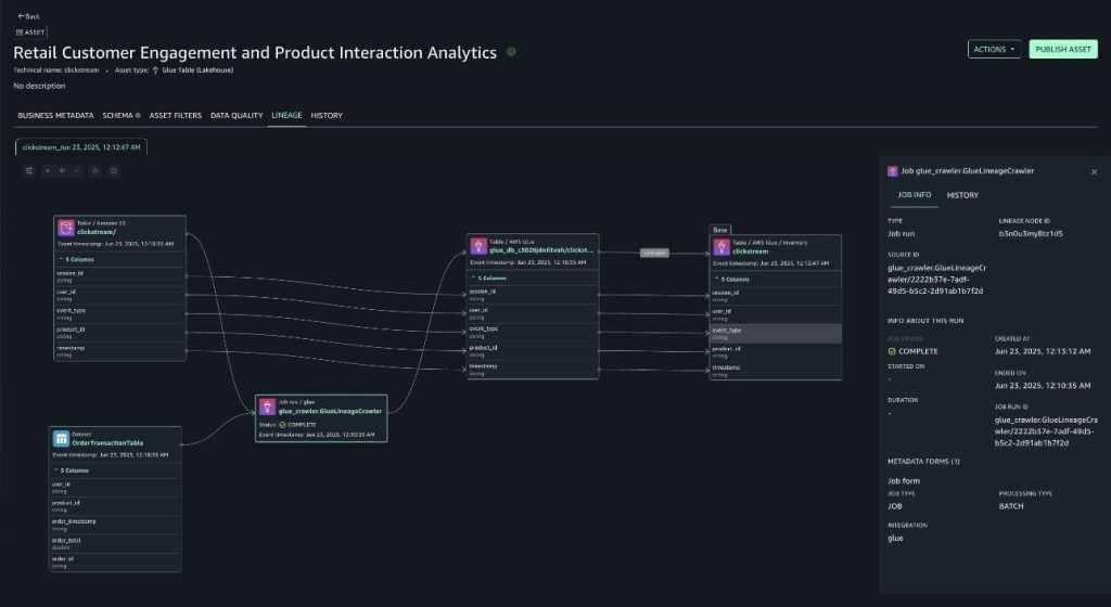

 Mohit Dawar is a Senior Software Engineer at Amazon Web Services (AWS) working on Amazon DataZone. Over the past 3 years, he has led efforts around the core metadata catalog, generative AI–powered metadata curation, and lineage visualization. He enjoys working on large-scale distributed systems, experimenting with AI to improve user experience, and building tools that make data governance feel effortless. Connect with him on LinkedIn:
  Jose Romero is a Senior Solutions Architect for Startups at Amazon Web Services (AWS) based in Austin, TX, US. He is passionate about helping customers architect modern platforms at scale for data, AI, and ML. As a former senior architect in AWS Professional Services, he enjoys building and sharing solutions for common complex problems so that customers can accelerate their cloud journey and adopt best practices. Connect with him on LinkedIn:
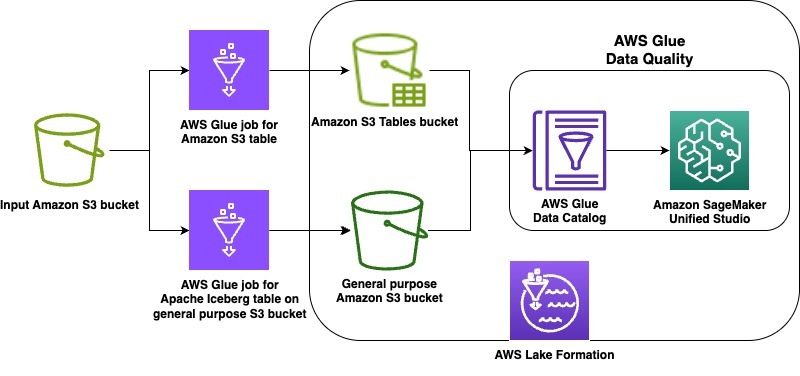

 Brody Pearman is a Senior Cloud Support Engineer at Amazon Web Services (AWS). He’s passionate about helping customers use AWS Glue ETL to transform and create their data lakes on AWS while maintaining high data quality. In his free time, he enjoys watching football with his friends and walking his dog.
 Shiv Narayanan is a Technical Product Manager for AWS Glue’s data management capabilities like data quality, sensitive data detection and streaming capabilities. Shiv has over 20 years of data management experience in consulting, business development and product management.
 Shriya Vanvari is a Software Developer Engineer in AWS Glue. She is passionate about learning how to build efficient and scalable systems to provide better experience for customers. Outside of work, she enjoys reading and chasing sunsets.
 Narayani Ambashta is an Analytics Specialist Solutions Architect at AWS, focusing on the automotive and manufacturing sector, where she guides strategic customers in developing modern data and AI strategies. With over 15 years of cross-industry experience, she specializes in big data architecture, real-time analytics, and AI/ML technologies, helping organizations implement modern data architectures. Her expertise spans across lakehouse architecture, generative AI, and IoT platforms, enabling customers to drive digital transformation initiatives. When not architecting modern solutions, she enjoys staying active through sports and yoga.
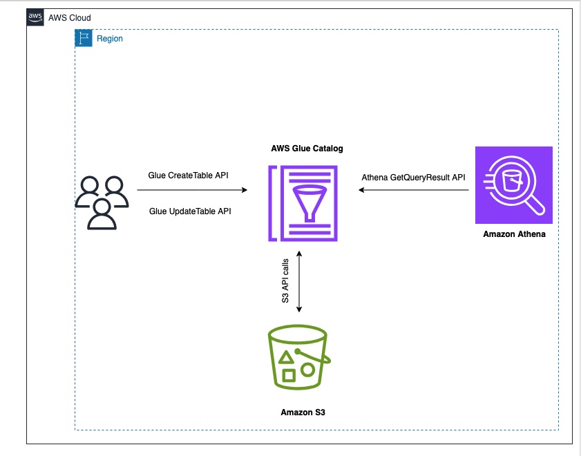
 Mohammad Sabeel Mohammad Sabeel is a Senior Cloud Support Engineer at Amazon Web Services (AWS) with over 14 years of experience in Information Technology (IT). As a member of the Technical Field Community (TFC) Analytics team, he is a Subject matter expert in Analytics services AWS Glue, Amazon Managed Workflows for Apache Airflow (MWAA), and Amazon Athena services. Sabeel provides expert guidance and technical support to enterprise and strategic customers, helping them optimize their data analytics solutions and overcome complex challenges. With deep subject matter expertise he enables organizations to build scalable, efficient, and cost-effective data processing pipelines.
 Indira Balakrishnan Indira Balakrishnan is a Principal Solutions Architect in the Amazon Web Services (AWS) Analytics Specialist Solutions Architect (SA) Team. She helps customers build cloud-based Data and AI/ML solutions to address business challenges. With over 25 years of experience in Information Technology (IT), Indira actively contributes to the AWS Analytics Technical Field community, supporting customers across various Domains and Industries. Indira participates in Women in Engineering and Women at Amazon tech groups to encourage girls to pursue STEM path to enter careers in IT. She also volunteers in early career mentoring circles.
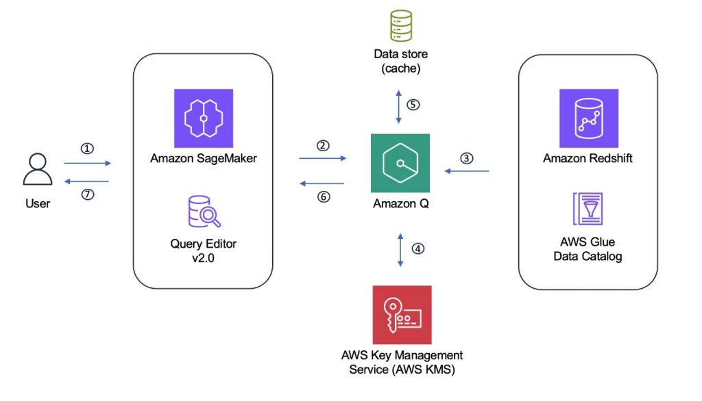
 Gregory Knowles is a data and AI specialist solution architect at AWS, focusing on the UK public sector. With extensive experience in cloud-based architectures, Greg guides public sector customers in implementing modern data solutions. His expertise spans governance, analytics, and AI/ML. Greg’s passion lies in accelerating transformation and innovation to improve productivity and outcomes. He has successfully led projects that moved data systems into the cloud, adopted new data architectures, and implemented AI at scale in production.
 Abhinav Tripathy is a Software Engineer and Security Guardian at AWS, where he develops Amazon Q generative SQL by combining machine learning, databases, and web systems. Abhinav is passionate about building scalable web systems from scratch that solve real customer challenges. Outside of work, he enjoys traveling, watching soccer, and playing badminton.
 Erol Murtezaoglu is a Technical Product Manager at AWS, is an inquisitive and enthusiastic thinker with a drive for self-improvement and learning. He has a strong and proven technical background in software development and architecture, balanced with a drive to deliver commercially successful products. Erol highly values the process of understanding customer needs and problems, in order to deliver solutions that exceed expectations.
 Peter Tsai is a Software Development Engineer at AWS, where he enjoys solving challenges in the design and performance of the AWS Glue runtime. In his leisure time, he enjoys hiking and cycling.
 Matt Su is a Senior Product Manager on the AWS Glue team. He enjoys helping customers uncover insights and make better decisions using their data with AWS Analytics services. In his spare time, he enjoys skiing and gardening.
 Sean McGeehan is a Software Development Engineer at AWS, where he builds features for the AWS Glue fulfillment system. In his leisure time, he explores his home of Philadelphia and work city of New York.


 Chiho Sugimoto is a Cloud Support Engineer on the AWS Big Data Support team. She is passionate about helping customers build data lakes using ETL workloads. She loves planetary science and enjoys studying the asteroid Ryugu on weekends.
 Saeed Barghi is a Sr. Specialist Solutions Architect at Amazon Web Services (AWS) specializing in architecting enterprise data platforms and AI solutions. Based in Melbourne, Australia, Saeed works with public sector customers in Australia and New Zealand and helps his customers build fit-for-purpose and future-proof data platforms and AI solutions.
 Miroslaw (Mick) Mioduszewski is the Director of Analytics at Revenue NSW Department of Customer service in NSW. He held multiple C-level roles in private and public companies as well as government, e.g. COO and CIO, as well as serving as company director. Mick holds computer science and business degrees, is a fellow of the Australian Institute of Company Directors and an industry fellow at the University of technology, Sydney.
 Moha Alsouli is a Public Sector Solutions Architect at Amazon Web Services (AWS) in Sydney. He is dedicated to supporting state and local government customers deliver citizen services, through solution design, reviews, optimisation, and architecture guidance. Moha is also specialising in generative artificial intelligence (AI) on AWS.


 Jeremy Spell is a Cloud Infrastructure Architect working with Amazon Web Services (AWS) Professional Services. He enjoys architecting and building solutions for customers. In his free time Jeremy makes Texas style BBQ, and spends time with his family and church community.
 Jeff Demuth is a solutions architect who joined Amazon Web Services (AWS) in 2016. He focuses on the geospatial community and is passionate about geographic information systems (GIS) and technology. Outside of work, Jeff enjoys traveling, building Internet of Things (IoT) applications, and tinkering with the latest gadgets.