Post Syndicated from Saman Irfan original https://aws.amazon.com/blogs/big-data/migrate-google-bigquery-to-an-open-lakehouse-on-aws-with-apache-iceberg/
Enterprises increasingly measure their readiness for AI by the readiness of their data, and that often means moving to an open lakehouse where data stays open and portable. The organizations moving fastest are the ones whose data gives them the flexibility to choose the engines and models that fit each workload. A tightly coupled, single-engine cloud data warehouse begins to hold them back. A generation of analytics tools was built inside vertically integrated systems, where the storage format, the catalog, and the query engine were fused into one vendor’s runtime. That design traded openness for convenience, and as generative AI, multi-engine analytics, and cross-team data sharing become the norm, the cost of that trade is rising. Increasingly, enterprises are choosing the opposite: an open, modular architecture where governance is defined once and enforced everywhere. This is the foundation for AI-ready data. It isn’t a new architecture to adopt, but an open lakehouse that keeps your data yours.
In this post, we explain why an open lakehouse architecture on AWS is the natural next step for organizations that are looking to future-proof their data architecture rather than re-architect onto another closed system. We then present the target architecture on AWS for migrating BigQuery workloads. Finally, we provide a step-by-step migration guide covering workload assessment, schema and query conversion, data movement strategies, and post-migration optimization to help you transition from BigQuery to an open lakehouse on AWS with confidence.
Why organizations are moving toward an open lakehouse
Open data, and the freedom to run engine of your choice. When data is held in a vendor’s proprietary format, it becomes difficult to use with other engines, tools, or AI models outside the vendor’s environment. Openness is what breaks it, but it comes in two degrees that are worth distinguishing. At the base is interoperability, which means many engines can reach the same data and it’s fast becoming table stakes now that even proprietary warehouses federate to open formats and query tables where they sit. Beyond that is portability: the freedom to take your data, your choice of engine, and your choice of AI model elsewhere without re-architecting. It’s the more durable property an open lakehouse is built to give you. Apache Iceberg is an open table format that removes these barriers: Iceberg compatible engines can read and write the same tables concurrently at petabyte scale while maintaining ACID compliance. On AWS, Apache Iceberg is a first-class citizen. Amazon Redshift, Amazon Athena, Amazon EMR, and AWS Glue all operate on one governed copy of the data in Amazon Simple Storage Service (Amazon S3). Because storage is decoupled from compute, you match the engine to the workload such as Athena for interactive SQL, Amazon Redshift for high-performance warehousing and business intelligence (BI), Amazon EMR for large-scale transformation, and Amazon SageMaker AI for machine learning (ML) without duplicating data or building extract, transform, and load (ETL) pipelines to shuffle it between systems. Interchangeability becomes a property of the architecture rather than something you engineer around.
Governance defined once, enforced across every engine. Openness doesn’t mean giving up control. On AWS, a single governance layer spans every engine that touches the data. The AWS Glue Data Catalog exposes an Apache Iceberg REST catalog endpoint that implements the Apache Iceberg REST Catalog open specification. AWS Lake Formation applies fine-grained access controls at the database, table, column, row, and cell level, defined once and enforced consistently whether a data engineer runs a Spark job on Amazon EMR, an analyst queries through Athena, or a data scientist trains a model in SageMaker AI. For discovery and sharing, you can use Amazon SageMaker Unified Studio to find, understand, and request access to governed data across the estate. Because the catalog follows an open specification rather than a single vendor’s runtime, governance travels with the data instead of locking it in.
A foundation that is AI-ready and model agnostic. The reason all this matters now is AI. Generative and agentic workloads are only as good as the data they can reach, and they perform best when data stays in open formats you fully control. But openness can’t stop at the data format. The intelligence layer matters too: the AI model, the semantic catalog, the enrichment layers, and the agents. An open foundation keeps both layers open. A single governed copy of open data sits in Amazon S3, and the same tables that serve BI and interactive analytics also feed Amazon SageMaker AI for model training and Amazon Bedrock and Amazon Bedrock AgentCore for generative and agentic work. You choose the foundation model (FM) that best fits your needs, with no extra copies to move or secure.
Target architecture: Open lakehouse on AWS
The following architecture diagram represents the recommended target state for organizations migrating BigQuery workloads to AWS and is especially well suited to customers wanting to build a unified, open data foundation. It’s built on Apache Iceberg as the foundational layer, with purpose-built consumption engines chosen per use case: Amazon Athena for interactive analytics, Amazon Redshift for BI reporting and dashboarding, and Amazon SageMaker AI for ML and agentic workloads, all on one governed copy of the data that stays open, interoperable, and portable.
The architecture follows the flow of data from left to right: source systems are ingested into an open lakehouse on Amazon S3, refined through medallion layers, and served to a diverse set of consumers such as BI tools, AI agents, and ML systems. It rests on four foundational pillars: open storage, purpose-built analytics, unified governance, and an integrated experience.
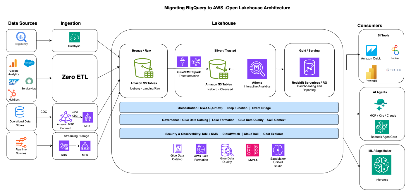
Figure 1: Open lakehouse target architecture on AWS, from source ingestion through the Amazon S3 Apache Iceberg storage layer to analytics, BI, and ML consumers
Ingestion
This is where it all begins. You must bring data from a variety of sources such as databases, software as a service (SaaS) applications, streaming systems, on-premises systems, IoT devices into your data lake.
- Bulk migration: For the initial BigQuery migration and other large batch transfers, use BigQuery’s EXPORT DATA statement to export tables to Google Cloud Storage (GCS) in Parquet format. Then use AWS DataSync to move Parquet files from Google Cloud Storage to Amazon S3. For more information, see Step 4.
- Zero-ETL: For SaaS and operational sources such as Google Analytics, Salesforce, SAP, ServiceNow, and HubSpot, Zero-ETL integrations land data directly in the lakehouse without building or maintaining custom pipelines.
- Change data capture (CDC): For operational data stores, Debezium connectors running on Amazon MSK Connect stream row-level changes into the lakehouse to keep it continuously current.
- Streaming: For real-time sources, Amazon Kinesis Data Streams and Amazon Managed Streaming for Apache Kafka (Amazon MSK) provide streaming storage that feeds directly into the raw layer.
Storage layer: Amazon S3 with Apache Iceberg
Amazon S3 serves as the central storage layer, providing virtually unlimited scalability, 99.999999999% (11 nines) of data durability, and multiple storage classes, so you can match cost to the access pattern. Data is stored in Apache Iceberg table format, which brings ACID transactions, schema evolution, time travel, and partition evolution to your data lake. Amazon S3 Tables, a capability of Amazon S3, provides a fully managed Apache Iceberg experience with automatic compaction, snapshot management, and optimization removing the undifferentiated heavy lifting of table maintenance.
Data is progressively refined through a medallion architecture, with each layer stored as Apache Iceberg tables on S3:
- Bronze/Raw: Ingested data lands here as-is, in Apache Iceberg format either on fully managed Amazon S3 Tables or as self-managed Apache Iceberg tables on Amazon S3.
- Silver/Trusted: Silver layer serves as single source of truth. AWS Glue and Amazon EMR Spark jobs transform, clean, and conform the raw data into trusted, query-ready Apache Iceberg tables. Amazon Athena provides serverless, interactive analytics directly against this layer for interactive exploration and data discovery.
- Gold/Serving: Amazon Redshift Serverless serves curated, business-ready data for dashboarding and reporting. Amazon Redshift is a first-class Apache Iceberg engine capable of managing the full Apache Iceberg table lifecycle (see Using Apache Iceberg tables with Amazon Redshift). Data can also be natively stored into Amazon Redshift Managed Storage for workloads that require increased performance for dashboarding and reporting use cases.
Governance: Unified across every engine
A unified foundation depends on governance that is defined once and enforced everywhere. The AWS Glue Data Catalog serves as the central metadata repository, and AWS Lake Formation provides fine-grained access control at the database, table, column, row, and cell level, enforced consistently whether data is accessed through Athena, Amazon Redshift, EMR, or SageMaker AI. AWS Glue Data Quality, a capability of AWS Glue, validates data as it moves through the layers and Amazon SageMaker Unified Studio provides a single integrated development environment for data discovery, SQL analytics, visual ETL, and artificial intelligence and machine learning (AI/ML) development all governed by the same Lake Formation permissions.
Consumers: One lakehouse, many workloads
Because data sits in open Apache Iceberg format under unified governance, a broad set of consumers can access a single source of truth without data movement:
- BI tools: Amazon Quick Suite, Looker, Power BI, and Tableau connect for dashboarding and reporting.
- AI agents: Agentic tooling such as MCP-based clients, Kiro, and Claude, along with Amazon Bedrock AgentCore, can reason over governed lakehouse data.
- ML/SageMaker: Amazon SageMaker AI trains models and serves inference directly against lakehouse data.
- Amazon SageMaker Unified Studio provides a single integrated development environment (IDE) for data exploration, SQL analytics, visual ETL, and AI/ML development. For organizations accustomed to a single-pane experience, Unified Studio addresses the concern of managing multiple services by providing one place to discover data, run queries, build dashboards, and develop ML models, all governed by the same Lake Formation permissions.
Data interoperability
The Apache Iceberg REST catalog endpoint of the AWS Glue Data Catalog, part of Amazon SageMaker Lakehouse, enables interoperability with third-party engines. Partners such as Snowflake and Databricks can read and write the same Apache Iceberg tables through that endpoint, so you choose the best tool for each job without duplicating data.
Cross-cutting layers: Orchestration, security, and observability
Two layers span the entire lakehouse rather than sitting at any single stage. An orchestration layer coordinates how data moves through the medallion layers: Amazon Managed Workflows for Apache Airflow (Amazon MWAA), AWS Step Functions, and Amazon EventBridge schedule and sequence ingestion, transformation, and load jobs across Bronze, Silver, and Gold.
A security and observability layer applies across every engine and layer. AWS Identity and Access Management (IAM) and AWS Key Management Service (AWS KMS) provide authentication, authorization, and encryption, while Amazon CloudWatch, AWS CloudTrail, and AWS Cost Explorer provide monitoring, audit logging, and cost visibility across the lakehouse.
Step-by-step migration guide
Migrating from BigQuery to an open lakehouse on AWS follows a structured, phased approach. Each phase builds confidence incrementally, so you can validate value before committing further.
Step 1: Assess and discover
Begin by evaluating your current BigQuery environment:
- Inventory workload: Catalog all datasets, tables, views, stored procedures, scheduled queries, and downstream consumers (BI tools, applications, ML pipelines). Name the consumers that most often need a decision: Looker Studio, Connected Sheets, scheduled queries, and any production service reading BigQuery directly.
- Classify query complexity: Analyze your SQL workloads to identify standard ANSI SQL (which migrates directly), BigQuery-specific syntax (such as
STRUCT,ARRAY,UNNEST, and JavaScript UDFs), and procedural logic in stored procedures. - Map data dependencies: Document which tools and applications read from and write to BigQuery. Identify upstream data sources (streaming, batch, CDC) and downstream consumers (dashboards, reports, ML models).
- Assess data volumes: Record active storage, long-term storage, data growth rates, and each dataset’s storage billing model (logical or physical) with its measured physical bytes. The compressed physical size can be a small fraction of the logical size and changes the storage cost estimate materially. This informs your S3 storage class strategy and cost modeling.
- Evaluate governance: Document current access controls, row-level security policies, and audit requirements. Map these to Lake Formation capabilities.
The output of this phase is a migration readiness report with per-table effort scoring, query complexity classification, and a recommended migration pattern.
AWS account teams and partners have metadata-driven assessment accelerators. They read only BigQuery metadata (schemas, INFORMATION_SCHEMA job history, view definitions, and routine signatures), not raw data. From that metadata, they produce a cost comparison with the projected savings, per-table migration effort scoring, a complexity classification for every view, routine, and observed query, and a map of every tool reading from or writing to BigQuery with how each one reconnects on AWS.
Reach out to your AWS account team for an initial assessment of moving BigQuery workload to an open lakehouse on AWS.
Step 2: Design target architecture
Based on your assessment findings, design the target-state architecture:
- Storage design: Define your S3 bucket structure with a multi-layer layout (raw, cleaned, and aggregated) aligned with data lifecycle best practices. For Apache Iceberg storage, we recommend Amazon S3 Tables for fully managed Apache Iceberg with automatic table maintenance and optimization and general-purpose S3 buckets with self-managed Apache Iceberg for cases that need granular control over table layout and compaction.
- Partitioning strategy: Design Iceberg partition schemes aligned to actual query access patterns. Use Iceberg’s native partitioning transforms (bucketing, time slicing) for optimal query pruning.
- Engine selection: Choose the engine from the workload you measured in Step 1. Amazon Athena fits estates that scan a moderate volume per day and tolerate a few seconds of latency whereas Amazon Redshift fits estates with sustained high concurrency, sub-second dashboard targets, or a daily scanned volume where warm compute is cheaper than paying per terabyte scanned. For large-scale data transformations, position Amazon EMR (including Amazon EMR Serverless) for complex, custom open source frameworks like Spark and Hive, or AWS Glue for serverless, integration-heavy ETL pipelines.
- Governance model: Design your AWS Lake Formation permission model to enforce granular database, table, column, and row-level access policies. Verify the architecture plans for multi-tenant access patterns if applicable.
- Ingestion architecture: Design data ingestion pipelines. Options include Zero-ETL integrations for operational data sources, Amazon Data Firehose for streaming data, and AWS Glue for batch ETL.
Step 3: Convert and validate (POC)
Pick a proof-of-concept slice, a handful of representative tables and the dashboards that read them, and convert BigQuery SQL, stored procedures, and data pipelines to their AWS equivalents.
- Schema conversion: A BigQuery dataset becomes an AWS Glue database when Athena is the engine, or an Amazon Redshift schema when Amazon Redshift is. The BigQuery project maps to your AWS account with its top-level namespace being the AWS Glue Data Catalog for Athena or to an Amazon Redshift database.
- SQL conversion: Convert BigQuery SQL dialect to ANSI SQL or engine-specific syntax. Common conversions include:
- BigQuery
STRUCTto Iceberg struct andARRAYto Iceberg list, and BigQuery JSON maps to a string column queried with JSON function when Athena is the engine and data is stored in Apache Iceberg format. For Amazon Redshift, the recommendation is to build the gold layer which is optimized for reporting use cases where data is flattened out for high-performance queries. If you need to store nested data inside Amazon Redshift, use the SUPER data type. - On Amazon Redshift, the target depends on where the data lands: for data stored natively in Amazon Redshift, BigQuery JSON maps to the
SUPERtype (queried with PartiQL), andSTRUCT/ARRAYare represented withinSUPER. - BigQuery
MERGEstatements to Athena or Amazon RedshiftMERGE INTO. Choose copy-on-write for tables updated in bulk and merge-on-read for frequently updated ones. - BigQuery JavaScript UDFs to a SQL expression where possible, otherwise an AWS Lambda-backed UDF on Athena (
USING EXTERNAL FUNCTION) or Amazon Redshift. - BigQuery scheduled queries to Amazon EventBridge Scheduler running Athena queries, Amazon Redshift scheduled queries in Query Editor v2, or dbt for anything that is a model. Chains of schedules become AWS Step Functions.
- BigQuery
- Pipeline conversion: Rebuild ETL pipelines using AWS Glue, dbt (with dbt-athena or dbt-redshift adapters), or Apache Spark on EMR.
- Validation: Run converted workloads against the slice. Compare row counts and checksums per table, query results for the dashboards on the slice, and run times against the agreed target, between BigQuery and AWS, to verify correctness.
BigQuery offers two pricing models for running queries. On-demand pricing is a scan-based model that charges $6.25 per terabyte of data scanned, while capacity-based pricing is a compute-based model that charges for the compute capacity used to run queries. Amazon Redshift is also compute-based, so if you currently run BigQuery on demand, its scan-based pricing is not directly comparable to Amazon Redshift’s compute-based pricing. Because the two models differ, benchmark a representative mix of queries on the target engine rather than a single query type.
A good practice is to run three tiers of queries and compare total cost and performance against your current BigQuery baseline: lightweight queries for simple lookups and aggregations, medium queries for moderate joins and transformations, and heavyweight queries for complex joins, window functions, and large scans. To build an accurate, workload-representative total cost of ownership (TCO), multiply each query tier by how often it runs, add storage costs, and produce a monthly figure you can compare directly to your current monthly BigQuery bill.
Step 4: Migrate data
Execute bulk data migration from BigQuery to Amazon S3 with Apache Iceberg:
- Use BigQuery’s EXPORT DATA statement to export tables to Google Cloud Storage (GCS) in Parquet format. For large datasets, partition exports by date or key ranges to parallelize the transfer.
- Use AWS DataSync to move Parquet files from Google Cloud Storage to Amazon S3. DataSync reads Google Cloud Storage directly through its S3-compatible XML API and writes the objects to your S3 bucket, with scheduling and incremental transfers built in. For most transfers you deploy a DataSync agent, either as a virtual machine in Google Cloud (closest to the source bucket) or as an Amazon Elastic Compute Cloud (Amazon EC2) instance in your virtual private cloud (VPC). DataSync Enhanced mode transfers between Google Cloud Storage and Amazon S3 run without an agent and offer higher performance and scalability.
- Create the Apache Iceberg tables in Athena or Amazon S3 Tables and load them from the exported Parquet with
CREATE TABLE AS SELECTorINSERT INTO, or register the existing files with Spark’sadd_filesprocedure on Amazon EMR or AWS Glue. - During the transition period, implement incremental data synchronization to keep AWS data current while BigQuery remains active. Use BigQuery’s change history functions (
APPENDSandCHANGES) for scheduled delta exports, change data capture (CDC) patterns, or Amazon AppFlow. - Apply for Google’s data transfer fee waiver before the bulk export starts: Google waives egress fees for customers leaving Google Cloud who request it through support and complete the export within the agreed window.
Step 5: Cutover and go-live
Execute production cutover with minimal disruption:
- Parallel run: Run workloads on both BigQuery and AWS simultaneously for a validation period. Compare outputs to confirm data consistency and query correctness.
- Redirect consumers: Every consumer takes one of three paths:
- Re-point: In this case, the tool stays the same, only its connection changes from BigQuery to Athena or Amazon Redshift (dbt, Fivetran, Tableau, Power BI, Looker). This is usually a JDBC/ODBC or connector update. Athena and Amazon Redshift both use the AWS Glue Iceberg REST catalog (IRC) endpoint to locate the physical Parquet files on Amazon S3. For more information, see Querying Apache Iceberg tables in Athena and Querying Apache Iceberg tables in Amazon Redshift.
- Rebuild: In this case, the workload has no direct AWS connection and is re-implemented on an AWS counterpart (BigQuery scheduled queries → Amazon Athena Saved Queries orchestrated by AWS Step Functions, or managed through Amazon EventBridge to run an ETL pipeline on a schedule, Dataform → dbt (using the Athena or Amazon Redshift connector), BigQuery ML → SageMaker AI or Amazon Redshift ML), Google Analytics 4 and Connected Sheets → Amazon AppFlow native connectors ingest the data (Google → AWS) into Amazon S3 or Amazon Redshift on a schedule. From S3, an AWS Glue or Athena step lands it in Apache Iceberg.
- Relay: In this case, the tool stays on Google Cloud for now and reads AWS data synced back to it (Connected Sheets, GA4 raw export).
Looker Studio, Connected Sheets, and scheduled queries are the consumers that most often need an explicit decision on which path to take.
- Validate end-to-end: Confirm that all dashboards, reports, scheduled jobs, and ML pipelines produce correct results.
- Decommission: After successful validation, decommission BigQuery resources and terminate cross-cloud data synchronization.
Step 6: Optimize and expand
Post-migration, optimize your lakehouse for performance and cost:
- Query optimization: On general-purpose buckets with self-managed Apache Iceberg, tune file size targets, compaction frequency, and sort orders to the actual query patterns whereas Amazon S3 Tables handles compaction and snapshot expiry automatically. Enable Athena query result reuse and Amazon Redshift materialized views for frequently accessed datasets.
- Cost optimization: Use S3 Intelligent-Tiering for infrequently accessed data, Athena workgroups and Amazon Redshift usage limits to control costs, and AWS Cost Explorer to monitor.
- Enable new capabilities: With data in open Apache Iceberg format on Amazon S3, you can take on use cases that were previously difficult or impossible:
- Train ML models directly on lakehouse data using SageMaker AI.
- Build generative AI applications with Amazon Bedrock Knowledge Bases.
- Implement real-time analytics with Amazon Data Firehose or Amazon Kinesis Data Streams writing Apache Iceberg tables to Amazon S3 Tables, or with Amazon Redshift streaming ingestion.
- Share Apache Iceberg tables with partner engines such as Snowflake and Databricks through the Apache Iceberg REST catalog endpoint.
Customer success: Yggdrasil Gaming
Yggdrasil Gaming, a global iGaming studio, migrated from BigQuery to an Apache Iceberg-based lakehouse on AWS, working with GOStack, an AWS Partner. The company had been operating dual-cloud infrastructure across AWS and Google Cloud, creating significant operational overhead that limited their ability to implement advanced analytics and AI/ML initiatives.
The migration followed a phased approach: establishing the lakehouse foundation on S3 with Apache Iceberg and AWS Glue Data Catalog, implementing real-time data ingestion using Debezium for change data capture, migrating processing pipelines to AWS Lambda and Amazon EMR, modernizing the transformation layer with dbt and Amazon Athena, and enabling governance through AWS Lake Formation.
The results were significant:
- 60 percent reduction in data processing costs.
- 75 percent improvement in analytics latency (from 2 hours to 30 minutes).
- Alleviated multi-cloud complexity by consolidating on AWS.
- Enabled AI/ML use cases including player behavior modeling and fraud detection.
For the full story, read Building a modern lakehouse architecture: Yggdrasil Gaming’s journey from BigQuery to AWS on the AWS Big Data Blog.
Customer success: Global technology leader performed zero-downtime GCP exit at petabyte scale
A global technology leader in the network security space migrated from Google BigQuery to AWS to reduce costs and enable streaming ingestion for network security analytics. Working with Quantiphi, an AWS Partner, the company migrated 10 core customer-facing applications across 3 regions with zero business downtime for more than 1,000 customers.
Highlights of the migration:
- Migrated over 1,000 BigQuery projects to Amazon Athena with Apache Iceberg on Amazon S3 (setting up over 5,000 Apache Iceberg tables).
- Key drivers: cost reduction (30 percent savings in cloud operational costs), streaming ingestion for security analytics, and regulatory alignment.
- Zero business downtime across a petabyte-scale migration spanning three AWS Regions, with minute-level data refresh meeting a 99.9 percent service level agreement (SLA).
- A full GCP exit consolidating entirely on AWS through Quantiphi’s Qatapult modernization and migration platform.
For the full story, read Engineering Excellence: How a Tech Leader Migrated to AWS with Zero Business Downtime (Quantiphi case study).
Conclusion
Migrating from BigQuery to an open lakehouse architecture on AWS with Apache Iceberg is an architectural change and a strategic investment in data openness, multi-engine flexibility, and AI readiness. By storing data in open formats on Amazon S3, governing it centrally through AWS Lake Formation, and accessing it with purpose-built engines, you build a data foundation that adapts to your evolving needs without vendor lock-in.
The phased migration approach (assess, design, convert, migrate, cutover, and optimize) means you can validate value at each step and maintain business continuity throughout the transition. Organizations like Yggdrasil Gaming have demonstrated that this migration can be completed in months, not years, with measurable cost savings and performance improvements.
To get started, explore the following resources:
- The lakehouse architecture of Amazon SageMaker
- Navigating architectural choices for a lakehouse using Amazon SageMaker
- A Systematic Approach for Analytics Services Migration from GCP to AWS