Post Syndicated from Miguel Chin original https://aws.amazon.com/blogs/big-data/how-olx-group-migrated-to-amazon-redshift-ra3-for-simpler-faster-and-more-cost-effective-analytics/

This is a guest post by Miguel Chin, Data Engineering Manager at OLX Group and David Greenshtein, Specialist Solutions Architect for Analytics, AWS.

OLX Group is one of the world’s fastest-growing networks of online marketplaces, operating in over 30 countries around the world. We help people buy and sell cars, find housing, get jobs, buy and sell household goods, and much more.

We live in a data-producing world, and as companies want to become data driven, there is the need to analyze more and more data. These analyses are often done using data warehouses. However, a common data warehouse issue with ever-growing volumes of data is storage limitations and the degrading performance that comes with it. This scenario is very familiar to us in OLX Group. Our data warehouse is built using Amazon Redshift and is used by multiple internal teams to power their products and data-driven business decisions. As such, it’s crucial to maintain a cluster with high availability and performance while also being storage cost-efficient.

In this post, we share how we modernized our Amazon Redshift data warehouse by migrating to RA3 nodes and how it enabled us to achieve our business expectations. Hopefully you can learn from our experience in case you are considering doing the same.

Status quo before migration

Here at OLX Group, Amazon Redshift has been our choice for data warehouse for over 5 years. We started with a small Amazon Redshift cluster of 7 DC2.8xlarge nodes, and as its popularity and adoption increased inside the OLX Group data community, this cluster naturally grew.

Before migrating to RA3, we were using a 16 DC2.8xlarge nodes cluster with a highly tuned workload management (WLM), and performance wasn’t an issue at all. However, we kept facing challenges with storage demand due to having more users, more data sources, and more prepared data. Almost every day we would get an alert that our disk space was close to 100%, which was about 40 TB worth of data.

Our usual method to solve storage problems used to be to simply increase the number of nodes. Overall, we reached a cluster size of 18 nodes. However, this solution wasn’t cost-efficient enough because we were adding compute capacity to the cluster even though computation power was underutilized. We saw this as a temporary solution, and we mainly did it to buy some time to explore other cost-effective alternatives, such as RA3 nodes.

Amazon Redshift RA3 nodes along with Redshift Managed Storage (RMS) provided separation of storage and compute, enabling us to scale storage and compute separately to better meet our business requirements.

Our data warehouse had the following configuration before the migration:

• 18 x DC2.8xlarge nodes
• 250 monthly active users, consistently increasing
• 10,000 queries per hour, 30 queries in parallel
• 40 TB of data, consistently increasing
• 100% disk space utilization

This cluster’s performance was generally good, ETL (extract, transform, and load) and interactive queries barely had any queue time, and 80% of them would finish in under 5 minutes.

Evaluating the performance of Amazon Redshift clusters with RA3 nodes

In this section, we discuss how we conducted a performance evaluation of RA3 nodes with an Amazon Redshift cluster.

Test environment

In order to be confident with the performance of the RA3 nodes, we decided to stress test them in a controlled environment before making the decision to migrate. To assess the nodes and find an optimal RA3 cluster configuration, we collaborated with AllCloud, the AWS premier consulting partner. The following figures illustrate the approach we took to evaluate the performance of RA3.

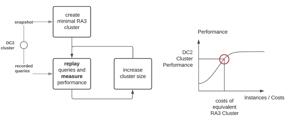
This strategy aims to replicate a realistic workload in different RA3 cluster configurations and compare them with our DC2 configuration. To do this, we required the following:

• A reference cluster snapshot – This ensures that we can replay any tests starting from the same state.
• A set of queries from the production cluster – This set can be reconstructed from the Amazon Redshift logs (STL_QUERYTEXT) and enriched by metadata (STL_QUERY). It should be noted that we only took into consideration SELECT and FETCH query types (to simplify this first stage of performance tests). The following chart shows what the profile of our test set looked like.

• A replay tool to orchestrate all the query operations – AllCloud developed a Python application for us for this purpose.

For more details about approach we used, including using the Amazon Redshift Simple Replay utility, refer to Compare different node types for your workload using Amazon Redshift.

Next, we picked which cluster configurations we wanted to test, which RA3 type, and how many nodes. For the specifications of each node type, refer to Amazon Redshift pricing.

First, we decided to test the same DC2 cluster we had in production as a way to validate our test environment, followed by RA3 clusters using RA3.4xlarge nodes with various numbers of nodes. We used RA3.4xlarge because it gives us more flexibility to fine-tune how many nodes we need compared to the RA3.16xlarge instance (1 x RA3.16xlarge node is equivalent to 4 x RA3.4xlarge nodes in terms of CPU and memory). With this in mind, we tested the following cluster configurations and used the replay tool to take measurements of the performance of each cluster.

		18 x DC2 (Reference)	18 x RA3 (Before Classic Resize)	18 x RA3	6 x RA3
Queries	Number	1560	1560	1560	1560
	Timeouts	–	25	66	127
Duration/s	Mean	1.214	1.037	1.167	1.921
	Std.	2.268	2.026	2.525	3.488
	Min.	0.003	0.000	0.002	0.002
	Q 25%	0.005	0.004	0.004	0.004
	Q 50%	0.344	0.163	0.118	0.183
	Q 75%	1.040	0.746	1.076	2.566
	Max.	25.411	15.492	19.770	19.132

These results show how the DC2 cluster compares with other RA3 configurations. For 50% of the faster queries (quantile 50%) they ran faster than on DC2. Regarding the number of RA3 nodes, six nodes were clearly slower, particularly noticeable on quantile 75% of query durations.

We used the following steps to deploy different clusters:

1. Use 18 x DC2.8xlarge, restored from the original snapshot (18 x DC2.8xlarge).
2. Take measurements 18 x DC2.
3. Use 18 x RA3.4xlarge, restored from the original snapshot (18 x DC2.8xlarge).
4. Take measurements 18 x RA3 (before classic resize).
5. Use 6 x RA3.4xlarge, classic resize from 18 x RA3.4xlarge.
6. Take snapshot from 6 x RA3.4xlarge.
7. Take measurements 6 x RA3.
8. Use 6 x RA3.4xlarge, restored from 6 x RA3.4xlarge snapshot.
9. Use 18 x RA3.4xlarge, elastic resize from 6 x RA3.4xlarge.
10. Take measurements 18x RA3.

Although these are promising results, there were some limitations in the test environment setup. We were concerned that we weren’t stressing the clusters enough, queries were only running in sequence using a single client, and the fact that we were using only SELECT and FETCH query types moved us away from a realistic workload. Therefore, we proceeded to the second stage of our tests.

Concurrency stress test

To stress the clusters, we changed our replay tool to run multiple queries in parallel. Queries extracted from the log files were queued with the same frequency as they were originally run in the reference cluster. Up to 50 clients take queries from the queue and send them to Amazon Redshift. The timing of all queries is recorded for comparison with the reference cluster.

The cluster performance is evaluated by measuring the temporal course of the query concurrency. If a cluster is equally performant as the reference cluster, the concurrency will closely follow the concurrency of the reference cluster. Queries pushed to the query queue are immediately picked up by a client and sent to the cluster. If the cluster isn’t capable of handling the queries as fast as the reference cluster, the number of running concurrent queries will increase when compared to the reference cluster. We also decided to keep concurrency scaling disabled during this test because we wanted to focus on node types instead of cluster features.

The following table shows the concurrent queries running on a DC2 and RA3 (both 18 nodes) with two different query test sets (3:00 AM and 1:00 PM). These were selected so we could test both our day and overnight workloads. 3:00 AM is when we have a peak of automated ETL jobs running, and 1:00 PM is when we have high user activity.

The median of running concurrent queries on the RA3 cluster is much higher than the DC2 one. This led us to conclude that a cluster of 18 RA3.4xlarge might not be enough to handle this workload reliably.

Concurrency	18 x DC2.8xlarge		18 x RA3.4xlarge
Starting	3:00 AM	1:00 PM	3:00 AM	1:00 PM
Mean	5	7	10	5
STD	11	13	7	4
25%	1	1	5	2
50%	2	2	8	4
75%	4	4	13	7
Max	50	50	50	27

RA3.16xlarge

Initially, we chose the RA3.4xlarge node type for more granular control in fine-tuning the number of nodes. However, we overlooked one important detail: the same instance type is used for worker and leader nodes. A leader node needs to manage all the parallel processing happening in the cluster, and a single RA3.4xlarge wasn’t enough to do so.

With this in mind, we tested two more cluster configurations: 6 x RA3.16xlarge and 8 x RA3.16xlarge, and once again measured concurrency. This time the results were much better; RA3.16xlarge was able to keep up with the reference concurrency, and the sweet spot seemed to be between 6–8 nodes.

Concurrency	18 x DC2.8xlarge		18 x RA3.4xlarge		6 x RA3.16xlarge	8 x RA3.16xlarge
Starting	3:00 AM	1:00 PM	3:00 AM	1:00 PM	3:00 AM	3:00 AM
Mean	5	7	10	5	3	1
STD	11	13	7	4	4	1
25%	1	1	5	2	2	0
50%	2	2	8	4	3	1
75%	4	4	13	7	4	2
Max	50	50	50	27	38	9

Things were looking better and our target configuration was now a 7 x RA3.16xlarge cluster. We were now confident enough to proceed with the migration.

The migration

Regardless of how excited we were to proceed, we still wanted to do a calculated migration. It’s best practice to have a playbook for migrations—a step-by-step guide on what needs to be done and also a contingency plan that includes a rollback plan. For simplicity reasons, we list here only the relevant steps in case you are looking for inspiration.

Migration plan

The migration plan included the following key steps:

1. Remove the DNS from the current cluster, in our case in Amazon Route 53. No users should be able to query after this.
2. Check if any sessions are still running a query, and decide to wait or stop it. This strongly indicates these users are using the direct cluster URL to connect.
   1. To check running sessions, use SELECT * FROM STV_SESSIONS.
   2. To check stopped sessions, use SELECT PG_TERMINATE_BACKEND(xxxxx);.
3. Create a snapshot of the DC2 cluster.
4. Pause the DC2 cluster.
5. Create an RA3 cluster from the snapshot with the following configuration:
   1. Node type – RA3.16xlarge
   2. Number of nodes – 7
   3. Database name – Same as the DC2
   4. Associated IAM roles – Same as the DC2
   5. VPC – Same as the DC2
   6. VPC security groups – Same as the DC2
   7. Parameter groups – Same as the DC2
6. Wait for SELECT COUNT(1) FROM STV_UNDERREPPED_BLOCKS to return 0. This is related to the hydration process of the cluster.
7. Point the DNS to the RA3 cluster.
8. Users can now query the cluster again.

Contingency plan

In case the performance of hourly and daily ETL is not acceptable, the contingency plan is triggered:

1. Add one more node to deal with the unexpected workload.
2. Increase the limit of concurrency scaling hours.
3. Reassess the parameter group.

Following this plan, we migrated from DC2 to RA3 nodes in roughly 3.5 hours, from stopping the old cluster to booting the new one and letting our processes fully synchronize. We then proceeded to monitor performance for a couple of hours. Storage capacity was looking great and everything was running smoothly, but we were curious to see how the overnight processes would perform.

The next morning, we woke up to what we dreaded: a slow cluster. We triggered our contingency plan and in the following few days we ended up implementing all three actions we had in the contingency plan.

Adding one extra node itself didn’t provide much help, however users did experience good performance during the hours concurrency scaling was on. The concurrency scaling feature allows Amazon Redshift to temporarily increase cluster capacity whenever the workload requires it. We configured it to allow a maximum of 4 hours per day—1 hour for free and 3 hours paid. We chose this particular value because price-wise it is equivalent to adding one more node (taking us to nine nodes) with the added advantage of only using and paying for it when the workload requires it.

The last action we took was related to the parameter group, in particular, the WLM. As initially stated, we had a manually fine-tuned WLM, but it proved to be inefficient for this new RA3 cluster. Therefore, we decided to try auto WLM with the following configuration.

Manual WLM before introducing auto WLM	Queue 1	Data Team ETL queue (daily and hourly), admin, monitoring, data quality queries
	Queue 2	Users queue (for both their ETL and ad hoc queries)
Auto WLM	Queue 1: Priority highest	Daily Data Team ETL queue
	Queue 2: Priority high	Admin queries
	Queue 3: Priority normal	User queries and hourly Data Team ETL
	Queue 4: Priority low	Monitoring, data quality queries

Manual WLM requires you to manually allocate a percentage of resources and define a number of slots per queue. Although this gives you resource segregation, it also means resources are constantly allocated and can go to waste if they’re not used. Auto WLM dynamically sets these variables depending on each queue’s priority and workload. This means that a query in the highest priority queue will get all the resources allocated to it, while lower priority queues will need to wait for available resources. With this in mind, we split our ETL depending on its priority: daily ETL to highest, hourly ETL to normal (to give a fair chance for user queries to compete for resources), and monitoring and data quality to low.

After applying concurrency scaling and auto WLM, we achieved stable performance for a whole week, and considered the migration a success.

Status quo after migration

Almost a year has passed since we migrated to RA3 nodes, and we couldn’t be more satisfied. Thanks to Redshift Managed Storage (RMS), our disk space issues are a thing of the past, and performance has been generally great compared to our previous DC2 cluster. We are now at 300 monthly active users. Cluster costs did increase due to the new node type and concurrency scaling, but we now feel prepared for the future and don’t expect any cluster resizing anytime soon.

Looking back, we wanted to have a carefully planned and prepared migration, and we were able to learn more about RA3 with our test environment. However, our experience also shows that test environments aren’t always bulletproof, and some details may be overlooked. In the end, these are our main takeaways from the migration to RA3 nodes:

• Pick the right node type according to your workload. An RA3.16xlarge cluster provides more powerful leader and worker nodes.
• Use concurrency scaling to provision more resources when the workload demands it. Adding a new node is not always the most cost-efficient solution.
• Manual WLM requires a lot of adjustments; using auto WLM allows for a better and fairer distribution of cluster resources.

Conclusion

In this post, we covered how OLX Group modernized our Amazon Redshift data warehouse by migrating to RA3 nodes. We detailed how we tested before migration, the migration itself, and the outcome. We are now starting to explore the possibilities provided by the RA3 nodes. In particular, the data sharing capabilities together with Redshift Serverless open the door for exciting architecture setups that we are looking forward to.

If you are going through the same storage issues we used to face with your Amazon Redshift cluster, we highly recommend migrating to RA3 nodes. Its RMS feature decouples the scalability of compute and storage power, providing a more cost-efficient solution.

Thanks for reading this post and hopefully you found it useful. If you’re going through the same scenario and have any questions, feel free to reach out.

---

About the author

Miguel Chin is a Data Engineering Manager at OLX Group, one of the world’s fastest-growing networks of trading platforms. He is responsible for managing a domain-oriented team of data engineers that helps shape the company’s data ecosystem by evangelizing cutting-edge data concepts like data mesh.

David Greenshtein is a Specialist Solutions Architect for Analytics at AWS with a passion for ETL and automation. He works with AWS customers to design and build analytics solutions enabling business to make data-driven decisions. In his free time, he likes jogging and riding bikes with his son.