Post Syndicated from Veliswa Boya original https://aws.amazon.com/blogs/aws/amazon-s3-storage-lens-adds-performance-metrics-support-for-billions-of-prefixes-and-export-to-s3-tables/
Today, we’re announcing three new capabilities for Amazon S3 Storage Lens that give you deeper insights into your storage performance and usage patterns. With the addition of performance metrics, support for analyzing billions of prefixes, and direct export to Amazon S3 Tables, you have the tools you need to optimize application performance, reduce costs, and make data-driven decisions about your Amazon S3 storage strategy.
New performance metric categories
S3 Storage Lens now includes eight new performance metric categories that help identify and resolve performance constraints across your organization. These are available at organization, account, bucket, and prefix levels. For example, the service helps you identify small objects in a bucket or prefix that can slow down application performance. This can be mitigated by batching small objects or using the Amazon S3 Express One Zone storage class for higher performance small object workloads.
To access the new performance metrics, you need to enable performance metrics in the S3 Storage Lens advanced tier when creating a new Storage Lens dashboard or editing an existing configuration.
| Metric category | Details | Use case | Mitigation |
| Read request size | Distribution of read request sizes (GET) by day | Identify dataset with small read request patterns that slow down performance | Small request: Batch small objects or use Amazon S3 Express One Zone for high-performance small object workloads |
| Write request size | Distribution of write request sizes (PUT, POST, COPY, and UploadPart) by day | Identify dataset with small write request patterns that slow down performance | Large request: Parallelize requests, use MPU or use AWS CRT |
| Storage size | Distribution of object sizes | Identify dataset with small small objects that slow down performance | Small object sizes: Consider bundling small objects |
| Concurrent PUT 503 errors | Number of 503s due to concurrent PUT operation on same object | Identify prefixes with concurrent PUT throttling that slow down performance | For single writer, modify retry behavior or use Amazon S3 Express One Zone. For multiple writers, use consensus mechanism or use Amazon S3 Express One Zone |
| Cross-Region data transfer | Bytes transferred and requests sent across Region, in Region | Identify potential performance and cost degradation due to cross-Region data access | Co-locate compute with data in the same AWS Region |
| Unique objects accessed | Number or percentage of unique objects accessed per day | Identify datasets where small subset of objects are being frequently accessed. These can be moved to higher performance storage tier for better performance | Consider moving active data to Amazon S3 Express One Zone or other caching solutions |
| FirstByteLatency (existing Amazon CloudWatch metric) | Daily average of first byte latency metric | The daily average per-request time from the complete request being received to when the response starts to be returned | |
| TotalRequestLatency (existing Amazon CloudWatch metric) | Daily average of Total Request Latency | The daily average elapsed per request time from the first byte received to the last byte sent |
How it works
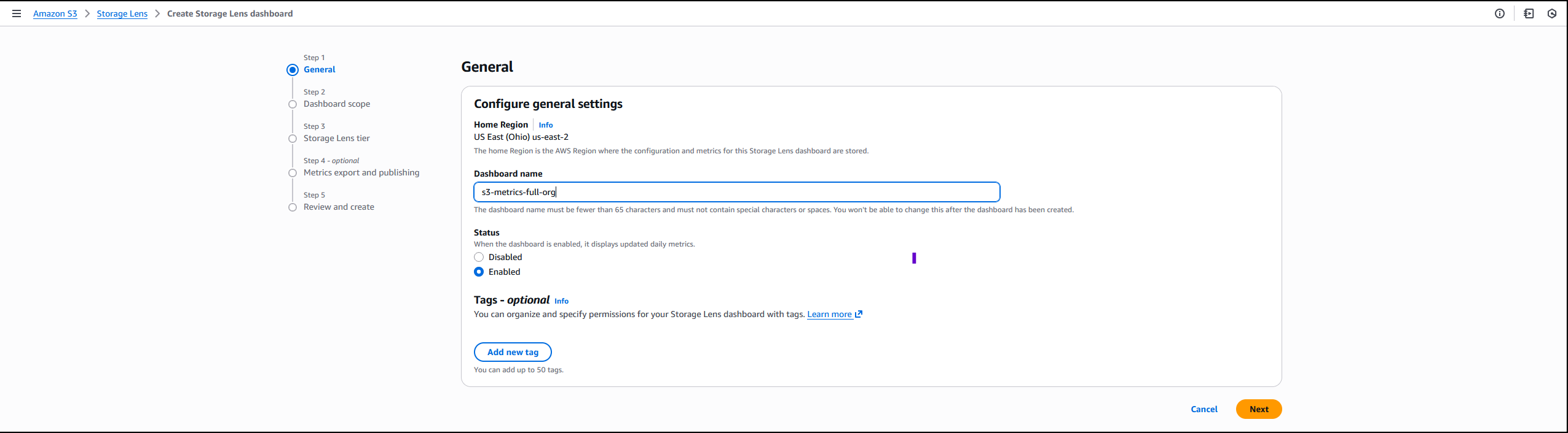
On the Amazon S3 console I choose Create Storage Lens dashboard to create a new dashboard. You can also edit an existing dashboard configuration. I then configure general settings such as providing a Dashboard name, Status, and the optional Tags. Then, I choose Next.
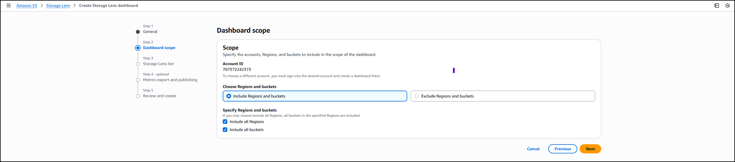
Next, I define the scope of the dashboard by selecting Include all Regions and Include all buckets and specifying the Regions and buckets to be included.
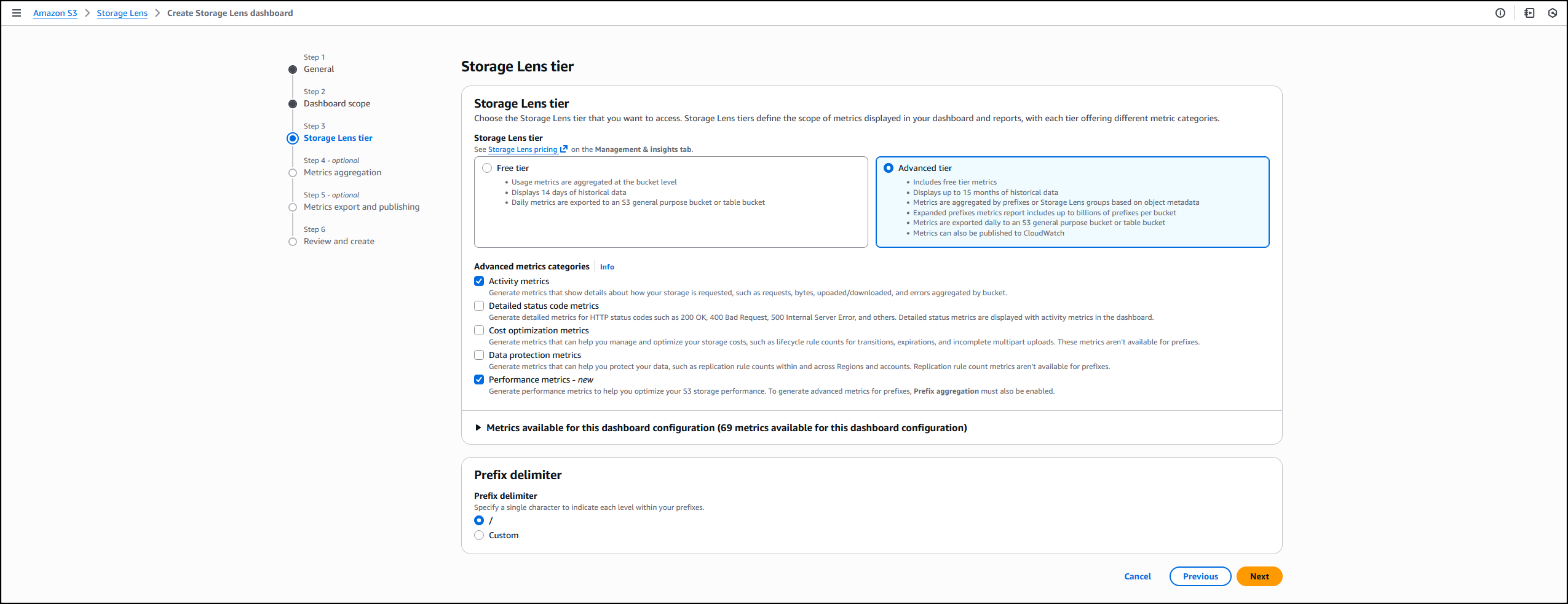
I opt in to the Advanced tier in the Storage Lens dashboard configuration, select Performance metrics, then choose Next.
Next, I select Prefix aggregation as an additional metrics aggregation, then leave the rest of the information as default before I choose Next.

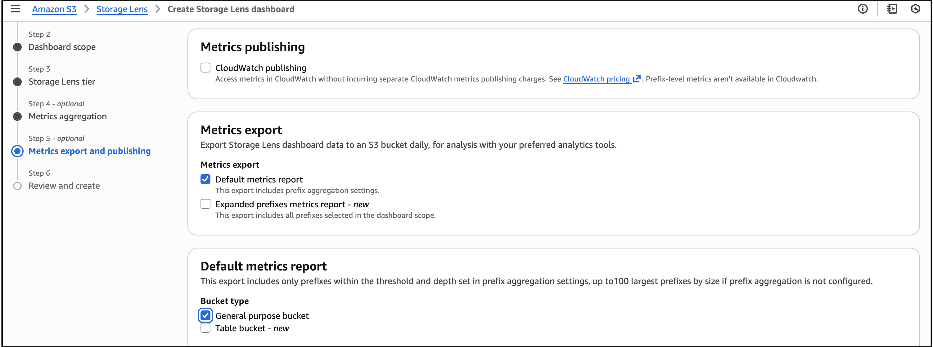
I select the Default metrics report, then General purpose bucket as the bucket type, and then select the Amazon S3 bucket in my AWS account as the Destination bucket. I leave the rest of the information as default, then select Next.
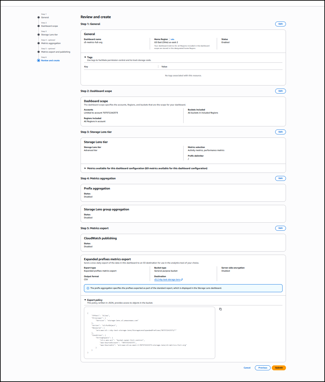
I review all the information before I choose Submit to finalize the process.
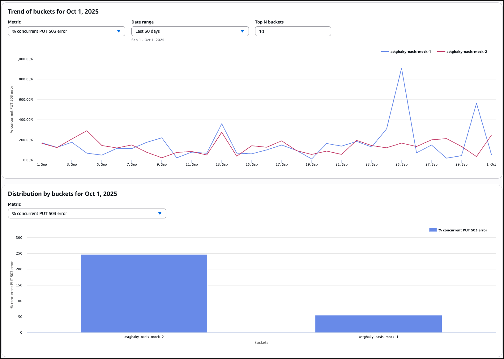
After it’s enabled, I’ll receive daily performance metrics directly in the Storage Lens console dashboard. You can also choose to export report in CSV or Parquet format to any bucket in your account or publish to Amazon CloudWatch. The performance metrics are aggregated and published daily and will be available at multiple levels: organization, account, bucket, and prefix. In this dropdown menu, I choose the % concurrent PUT 503 error for the Metric, Last 30 days for the Date range, and 10 for the Top N buckets.

The Concurrent PUT 503 error count metric tracks the number of 503 errors generated by simultaneous PUT operations to the same object. Throttling errors can degrade application performance. For a single writer, modify retry behavior or use higher performance storage tier such as Amazon S3 Express One Zone to mitigate concurrent PUT 503 errors. For multiple writers scenario, use a consensus mechanism to avoid concurrent PUT 503 errors or use higher performance storage tier such as Amazon S3 Express One Zone.
Complete analytics for all prefixes in your S3 buckets
S3 Storage Lens now supports analytics for all prefixes in your S3 buckets through a new Expanded prefixes metrics report. This capability removes previous limitations that restricted analysis to prefixes meeting a 1% size threshold and a maximum depth of 10 levels. You can now track up to billions of prefixes per bucket for analysis at the most granular prefix level, regardless of size or depth.
The Expanded prefixes metrics report includes all existing S3 Storage Lens metric categories: storage usage, activity metrics (requests and bytes transferred), data protection metrics, and detailed status code metrics.
How to get started
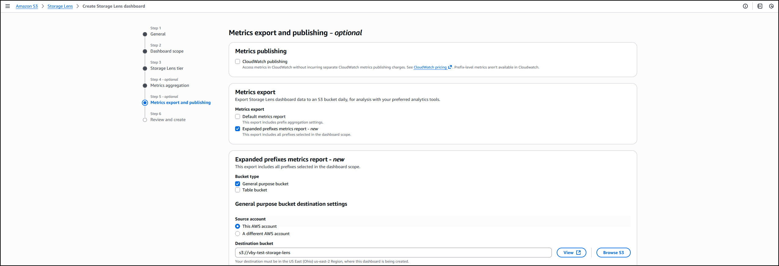
I follow the same steps outlined in the How it works section to create or update the Storage Lens dashboard. In Step 4 on the console, where you select export options, you can select the new Expanded prefixes metrics report. Thereafter, I can export the expanded prefixes metrics report in CSV or Parquet format to any general purpose bucket in my account for efficient querying of my Storage Lens data.
Good to know
This enhancement addresses scenarios where organizations need granular visibility across their entire prefix structure. For example, you can identify prefixes with incomplete multipart uploads to reduce costs, track compliance across your entire prefix structure for encryption and replication requirements, and detect performance issues at the most granular level.
Export S3 Storage Lens metrics to S3 Tables
S3 Storage Lens metrics can now be automatically exported to S3 Tables, a fully managed feature on AWS with built-in Apache Iceberg support. This integration provides daily automatic delivery of metrics to AWS managed S3 Tables for immediate querying without requiring additional processing infrastructure.
How to get started
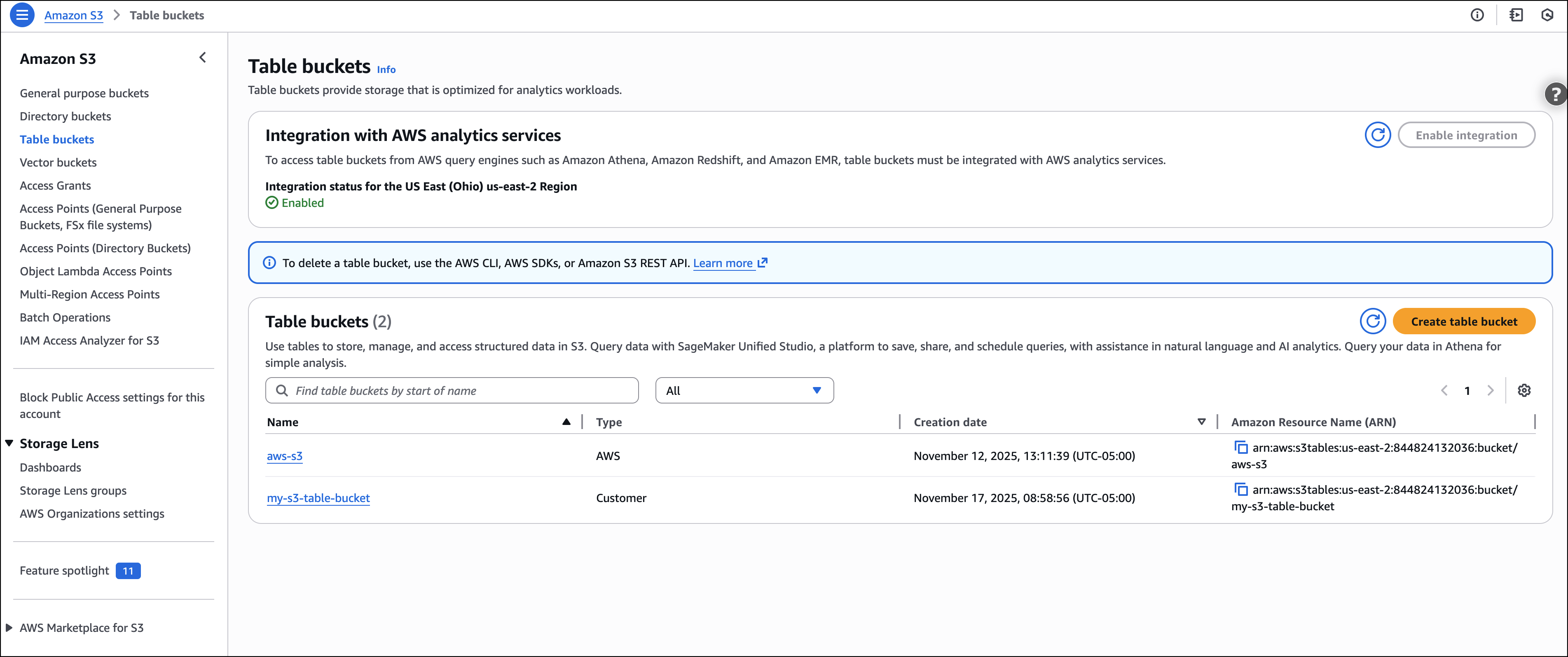
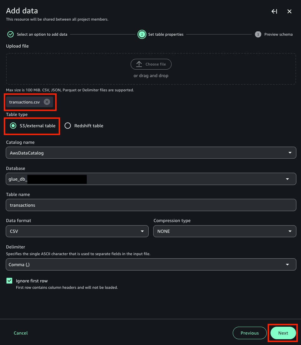
I start by following the process outlined in Step 5 on the console, where I choose the export destination. This time, I choose Expanded prefixes metrics report. In addition to General purpose bucket, I choose Table bucket.
The new Storage Lens metrics are exported to new tables in an AWS managed bucket aws-s3.
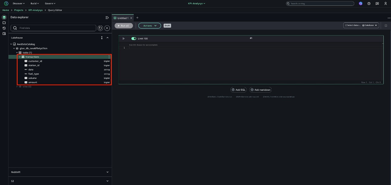
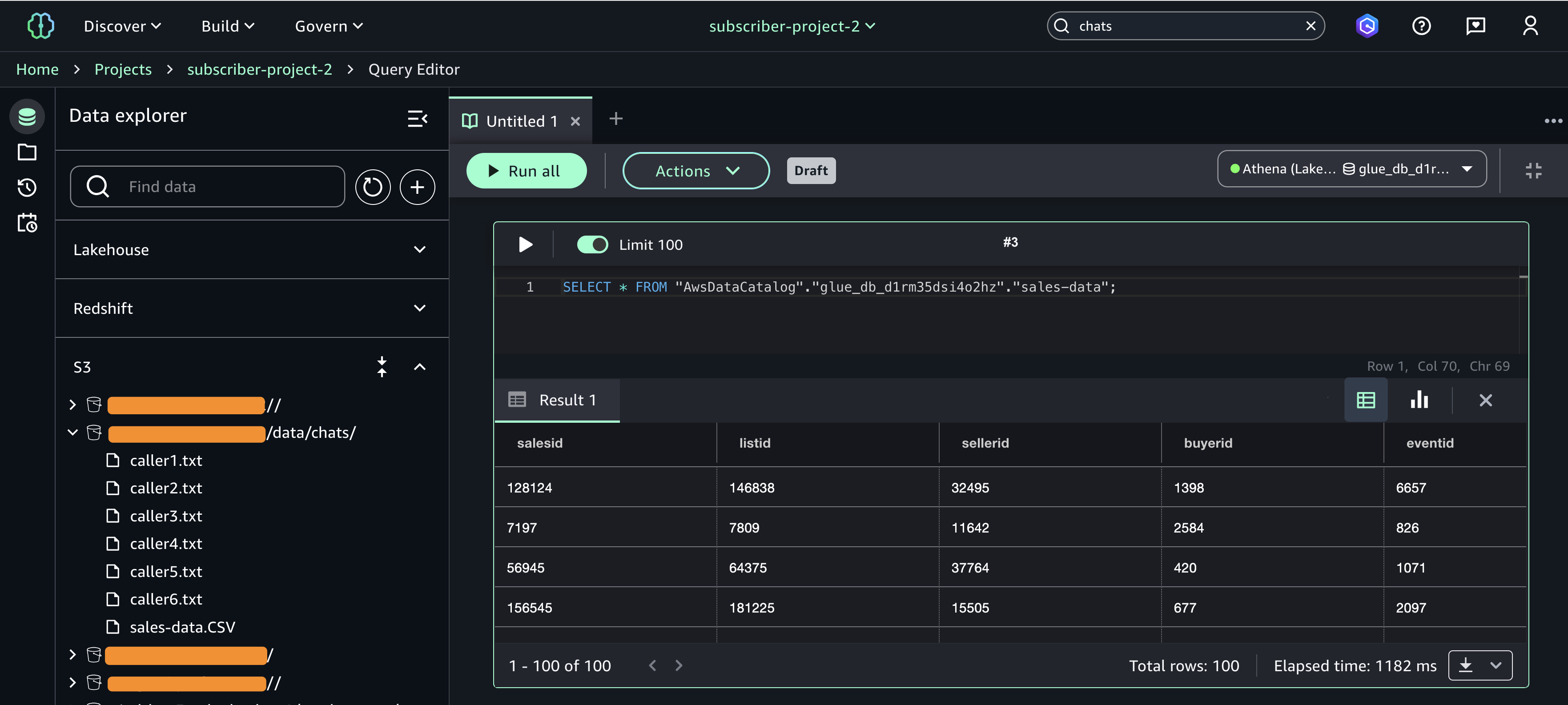
I select the expanded_prefixes_activity_metrics table to view API usage metrics for expanded prefix reports.
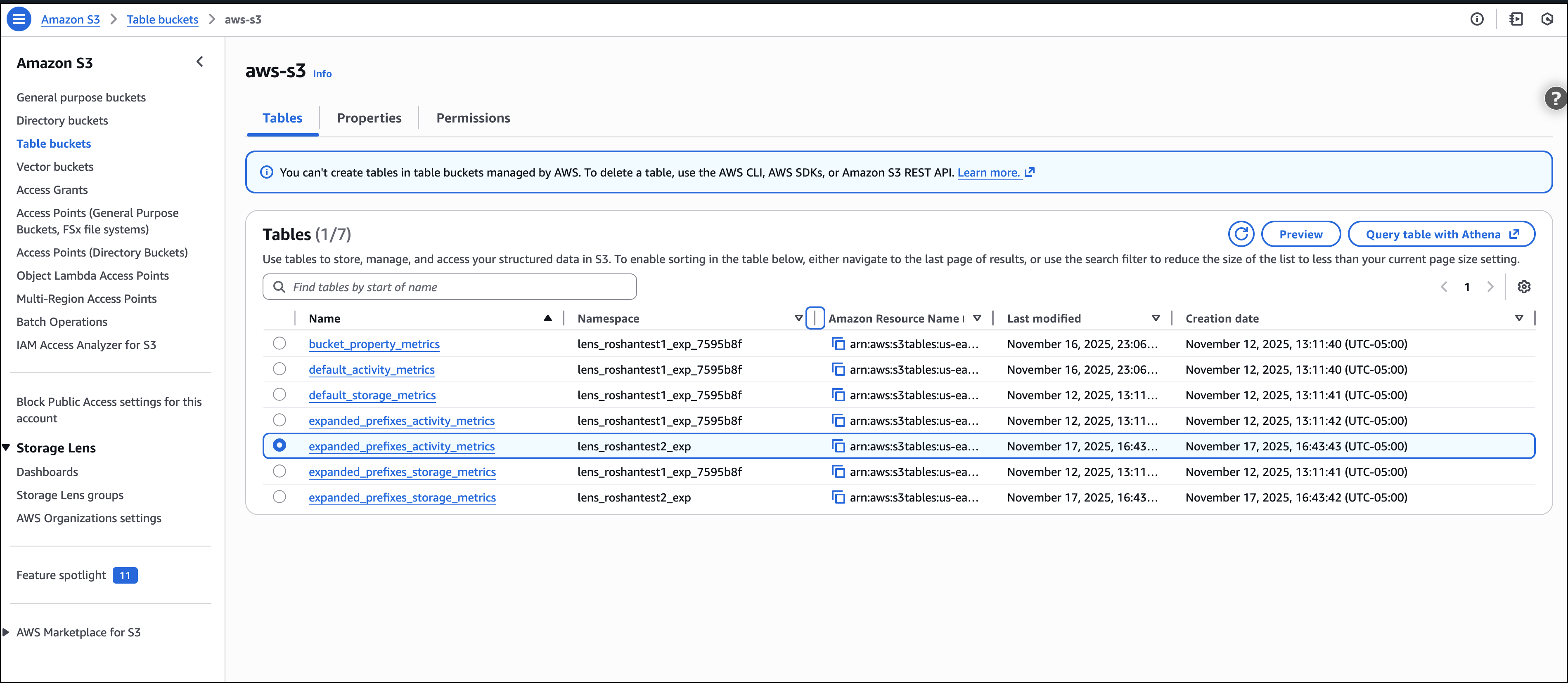
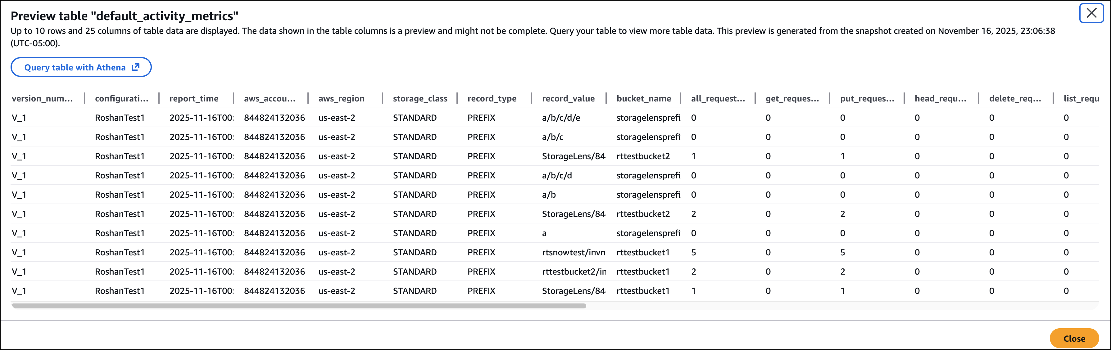
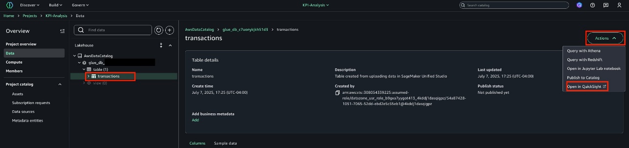
I can preview the table on the Amazon S3 console or use Amazon Athena to query the table.
Good to know
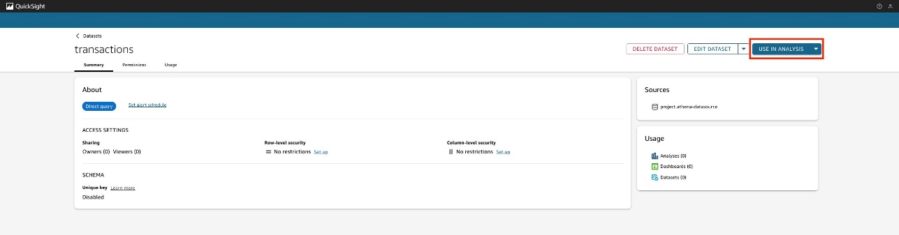
S3 Tables integration with S3 Storage Lens simplifies metric analysis using familiar SQL tools and AWS analytics services such as Amazon Athena, Amazon QuickSight, Amazon EMR, and Amazon Redshift, without requiring a data pipeline. The metrics are automatically organized for optimal querying, with custom retention and encryption options to suit your needs.
This integration enables cross-account and cross-Region analysis, custom dashboard creation, and data correlation with other AWS services. For example, you can combine Storage Lens metrics with S3 Metadata to analyze prefix-level activity patterns and identify objects in prefixes with cold data that are eligible for transition to lower-cost storage tiers.
For your agentic AI workflows, you can use natural language to query S3 Storage Lens metrics in S3 Tables with the S3 Tables MCP Server. Agents can ask questions such as ‘which buckets grew the most last month?’ or ‘show me storage costs by storage class’ and get instant insights from your observability data.
Now available
All three enhancements are available in all AWS Regions where S3 Storage Lens is currently offered (except the China Regions and AWS GovCloud (US)).
These features are included in the Amazon S3 Storage Lens Advanced tier at no additional charge beyond standard advanced tier pricing. For the S3 Tables export, you pay only for S3 Tables storage, maintenance, and queries. There is no additional charge for the export functionality itself.
To learn more about Amazon S3 Storage Lens performance metrics, support for billions of prefixes, and export to S3 Tables, refer to the Amazon S3 user guide. For pricing details, visit the Amazon S3 pricing page.


 Ramon Lopez is a Principal Solutions Architect for Amazon QuickSight. With many years of experience building BI solutions and a background in accounting, he loves working with customers, creating solutions, and making world-class services. When not working, he prefers to be outdoors in the ocean or up on a mountain.
 Leonardo Gomez is a Principal Analytics Specialist Solutions Architect at AWS. He has over a decade of experience in data management, helping customers around the globe address their business and technical needs. Connect with him on


 Enrique Salgado Hernández is a Senior Specialist Solutions Architect at AWS with more than 10 years of experience working in the cloud. He specializes in designing and implementing large-scale analytics architectures across various industry sectors. He is passionate about working with customers to solve their problems by supporting them during their cloud journey.
 Angel Conde Manjon is a Senior EMEA Data & AI PSA, based in Madrid. He previously worked on research related to data analytics and AI in diverse European research projects. In his current role, Angel helps partners develop businesses centered on data and AI.
 Donatas Kuchalskis is a Cloud Operations Architect at AWS, based in London, focusing on Financial Services customers in the UK. He helps customers optimize their AWS environments for cost, security, and resiliency while providing strategic cloud guidance. Prior to this role, he served as a Prototyping Architect specializing in Big Data and as a Specialist Solutions Architect for Retail. Before joining AWS, Donatas spent 6 years as a technical consultant in the retail sector.
 Jumana Nagaria is a Prototyping Architect at AWS. She builds innovative prototypes with customers to solve their business challenges. She is passionate about cloud computing and data analytics. Outside of work, Jumana enjoys travelling, reading, painting, and spending quality time with friends and family.


 Vetri Natarajan is a Specialist Solutions Architect for Amazon QuickSight. Vetri has 15 years of experience implementing enterprise business intelligence (BI) solutions and greenfield data products. Vetri specializes in integration of BI solutions with business applications and enable data-driven decisions.
 Ismael Murillo is a Solutions Architect for Amazon QuickSight. Before joining AWS, Ismael worked in Amazon Logistics (AMZL) with delivery station management, delivery service providers, and our customer actively in the field. Ismael focused on last mile delivery and delivery success. He designed and implemented many innovative solutions to help reduce cost, influence delivery success. He is also a United States Army Veteran, where he served for eleven years.

 Lead FinOps Engineer at BMW Group and has a strong background in data engineering, AI, and FinOps. He focuses on driving cloud efficiency initiatives and fostering a cost-aware culture within the company to leverage the cloud sustainably.
 Selman Ay is a Data Architect specializing in end-to-end data solutions, architecture, and AI on AWS. Outside of work, he enjoys playing tennis and engaging outdoor activities.
 Cizer Pereira is a Senior DevOps Architect at AWS Professional Services. He works closely with AWS customers to accelerate their journey to the cloud. He has a deep passion for cloud-based and DevOps solutions, and in his free time, he also enjoys contributing to open source projects.


 Leo Ramsamy is a Platform Architect specializing in data and analytics for ANZ’s Institutional division. He focuses on modern data practices, including Data Mesh architecture, data governance, quality management, and observability. His work aligns data strategies with business goals, improving accessibility and enabling better decision-making across ANZ.
 Srinivasan Kuppusamy is a Senior Cloud Architect – Data at AWS ProServe, where he helps customers solve their business problems using the power of AWS Cloud technology. His areas of interests are data and analytics, data governance, and AI/ML.
 Rada Stanic is a Chief Technologist at Amazon Web Services, where she helps ANZ customers across different segments solve their business problems using AWS Cloud technologies. Her special areas of interest are data analytics, machine learning/AI, and application modernization.


 Boon Lee Eu is a Senior Technical Account Manager at Amazon Web Services (AWS). He works closely and proactively with Enterprise Support customers to provide advocacy and strategic technical guidance to help plan and achieve operational excellence in AWS environment based on best practices. Based in Singapore, Boon Lee has over 20 years of experience in IT & Telecom industries.
 Kyara Labrador is a Sr. Analytics Specialist Solutions Architect at Amazon Web Services (AWS) Philippines, specializing in big data and analytics. She helps customers in designing and implementing scalable, secure, and cost-effective data solutions, as well as migrating and modernizing their big data and analytics workloads to AWS. She is passionate about empowering organizations to unlock the full potential of their data.
 Vikas Omer is the Head of Data & AI Solution Architecture for ASEAN at Amazon Web Services (AWS). With over 15 years of experience in the data and AI space, he is a seasoned leader who leverages his expertise to drive innovation and expansion in the region. Vikas is passionate about helping customers and partners succeed in their digital transformation journeys, focusing on cloud-based solutions and emerging technologies.


 Srividya Parthasarathy is a Senior Big Data Architect on the AWS Lake Formation team. She enjoys building data mesh solutions and sharing them with the community.
 Maneesh Sharma is a Senior Database Engineer at AWS with more than a decade of experience designing and implementing large-scale data warehouse and analytics solutions. He collaborates with various Amazon Redshift Partners and customers to drive better integration.
 Poulomi Dasgupta is a Senior Analytics Solutions Architect with AWS. She is passionate about helping customers build cloud-based analytics solutions to solve their business problems. Outside of work, she likes travelling and spending time with her family.


 Ayush Agrawal is a Startups Solutions Architect from Gurugram, India with 11 years of experience in Cloud Computing. With a keen interest in AI, ML, and Cloud Security, Ayush is dedicated to helping startups navigate and solve complex architectural challenges. His passion for technology drives him to constantly explore new tools and innovations. When he’s not architecting solutions, you’ll find Ayush diving into the latest tech trends, always eager to push the boundaries of what’s possible.
 Fraser Sequeira is a Solutions Architect with AWS based in Mumbai, India. In his role at AWS, Fraser works closely with startups to design and build cloud-native solutions on AWS, with a focus on analytics and streaming workloads. With over 10 years of experience in cloud computing, Fraser has deep expertise in big data, real-time analytics, and building event-driven architecture on AWS.


