Post Syndicated from Shivani Mehendarge original https://aws.amazon.com/blogs/big-data/schedule-notebook-runs-in-amazon-sagemaker-unified-studio/

If you build notebooks for recurring tasks such as daily customer analysis, weekly report generation, or data quality checks in Amazon SageMaker Unified Studio, you’ve likely wanted to run them automatically on a schedule. Until now, there wasn’t a native way to do this. Teams had to manage orchestration separately, even though the interactive notebook experience was already in place. Now, notebook scheduling is available, so you can configure your production workloads to run automatically with minimal manual intervention.

In this post, we walk you through the new scheduling and orchestrating capabilities for notebooks in Amazon SageMaker Unified Studio. You will learn how to:

• Trigger on-demand background runs, such as a model re-training job, without waiting at your desk.
• Create recurring schedules for tasks such as nightly data freshness checks or weekly business reviews.
• Parameterize notebooks so a single template can generate reports across different AWS Regions or customer segments.
• Orchestrate multi-notebook workflows where one notebook’s output feeds into the next. For example, an extract, transform, and load (ETL) pipeline followed by a summary dashboard refresh.
• Debug failed runs with AI-assisted troubleshooting.

Sample use case overview

In this walkthrough, you will take on the role of a logistics analyst who monitors shipping performance across carriers. The notebook loads shipping data from the ShippingLogs.csv dataset, identifies late deliveries, and generates a performance summary. You want to run this notebook every morning without manual intervention, reuse it across different carriers, and know when something goes wrong.

You will start by running a notebook in the background and viewing the results. Next, you will create a recurring schedule for daily runs, then parameterize the notebook to generate reports for different carriers. You will also orchestrate the notebook in a multi-step workflow and debug a failed run using AI-assisted troubleshooting.

Prerequisites

Before you begin, you need:

• An Amazon SageMaker Unified Studio project with Notebooks enabled. See Set up IAM-based domains for permission requirements.
• A sample dataset. We use the ShippingLogs.csv dataset, which contains shipping data including estimated and actual delivery times, carriers, and origins. You can download it from the Workshop Studio (the file is named ShippingLogs.csv on the linked page).

Setting up the notebook

Start by creating a new notebook in your SageMaker Unified Studio project. If you haven’t already, upload the ShippingLogs.csv file under the Shared tab in the Files panel.

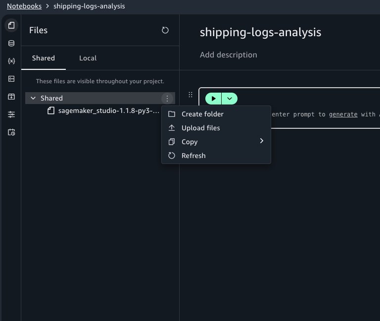
In the first cell, we load and explore the dataset. To reference the file in code, select the file in the Shared tab and copy the Amazon Simple Storage Service (Amazon S3) URI shown in the file details. Alternatively, you can reference it with this code:

import pandas as pd
from sagemaker_studio import Project

# Initialize the project
proj = Project()

# Get the S3 root path
s3_root = proj.s3.root

df = pd.read_csv(s3_root + '/ShippingLogs.csv')
df.head()

The dataset contains columns including Carrier, ActualShippingDays, ExpectedShippingDays, ShippingOrigin, ShippingPriority, and OnTimeDelivery. Add a second cell to analyze shipping performance for a single carrier:

import matplotlib.pyplot as plt

carrier_data = df[df['Carrier'] == 'GlobalFreight']
# Flag late deliveries
carrier_data['is_late'] = carrier_data['ActualShippingDays'] > carrier_data['ExpectedShippingDays']
late_pct = carrier_data['is_late'].mean() * 100
# Visualize actual vs expected shipping days
plt.figure(figsize=(12, 4))
plt.hist(carrier_data['ActualShippingDays'] - carrier_data['ExpectedShippingDays'], bins=20, edgecolor='black')
plt.axvline(x=0, color='red', linestyle='--', label='On time')
plt.title(f'Shipping Delay Distribution - GlobalFreight ({late_pct:.1f}% late)')
plt.xlabel('Days Over Expected')
plt.ylabel('Number of Shipments')
plt.legend()
plt.show()

With the notebook working interactively, you’re ready to automate it.

Running a notebook asynchronously

To trigger an asynchronous run, open your notebook. In the notebook header, choose the menu on the Run all button, and then choose Run in background.

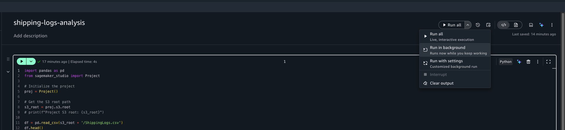
This captures a snapshot of the notebook in its current state and starts a run on a separate dedicated compute. You can continue working on other tasks or close the browser entirely. Your interactive session isn’t affected.

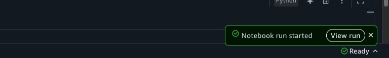
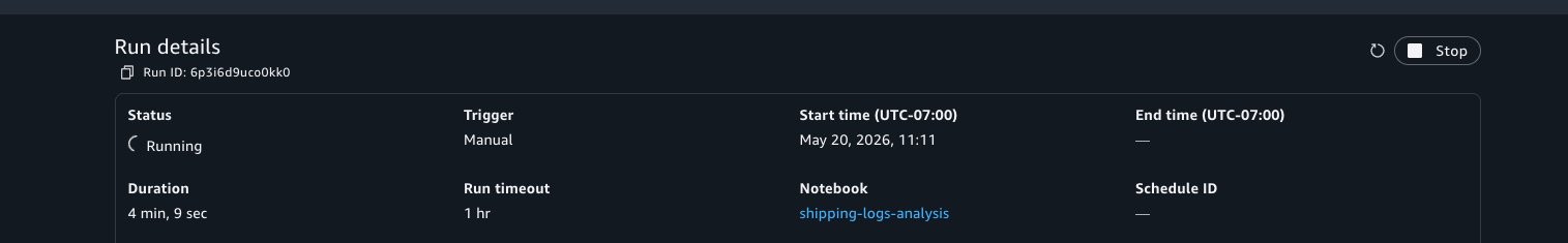
You will see a notification at the bottom of your screen confirming that the run started. To check the status of your run, choose View Run in the notification. This opens a view showing every background and scheduled run with its status, duration, and a link to view the full output.

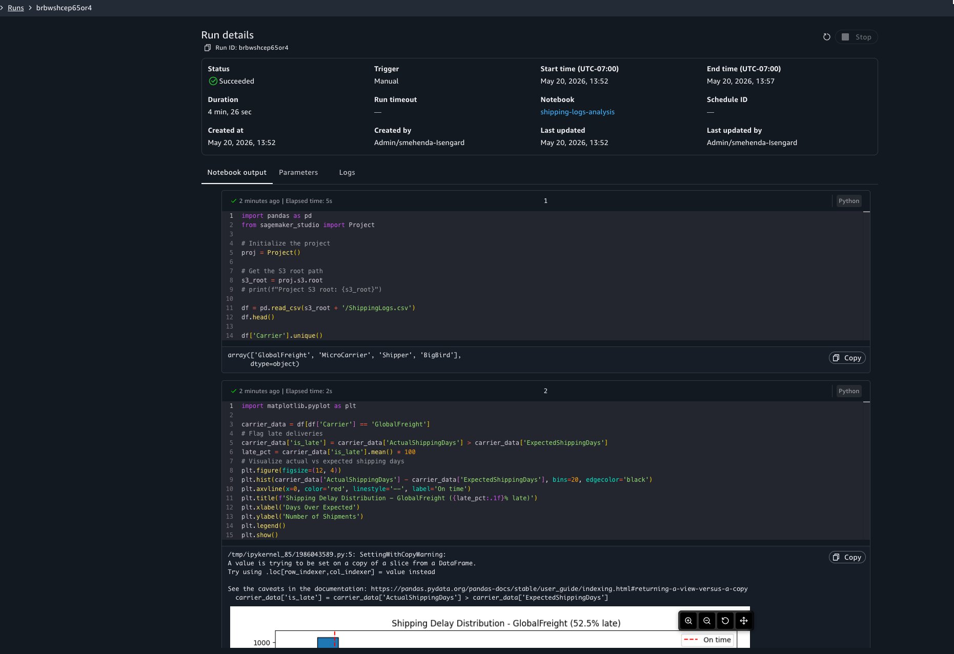
You can choose to view the run details at any point to view results as cells run. The run details include three tabs:

• Output: The notebook in read-only mode with cell results rendered, including dataframe outputs, visualizations, and print statements.
• Parameters: The parameter values used for this run.
• Logs: Run logs for debugging.

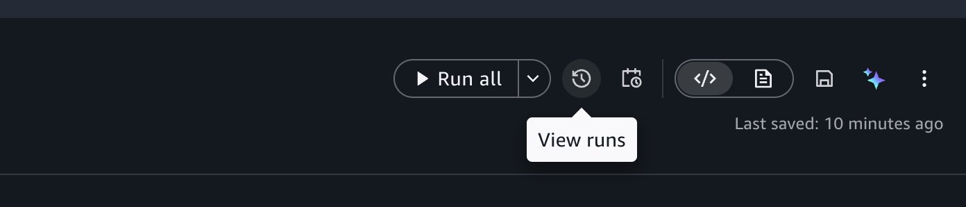
You can also access past runs by selecting the View Runs option in the notebook header.

Stopping an in-progress run

If you need to cancel a run, open the run, and choose Stop. The run terminates, and its status updates to reflect the cancellation.

What to know about background runs

Compute: Each background run uses its own dedicated compute, separate from your interactive session. Your interactive work isn’t interrupted.

Packages: The packages that you install through the notebook’s package manager will be available in your background runs. When you use !pip install in code cells, the asynchronous run installs those packages as well.

Local files: Background runs can’t access files stored locally in your notebook environment. Reference data from your project’s shared storage (Amazon S3) or connected data sources instead.

Startup time: Expect a few minutes of startup time while compute is provisioned and your environment is prepared.

Creating a recurring schedule

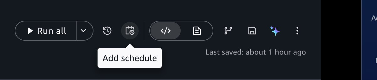
Now that you’ve confirmed asynchronous runs work correctly, you can automate the notebook on a schedule. Choose the schedule icon in the notebook header to open the schedule creation form.

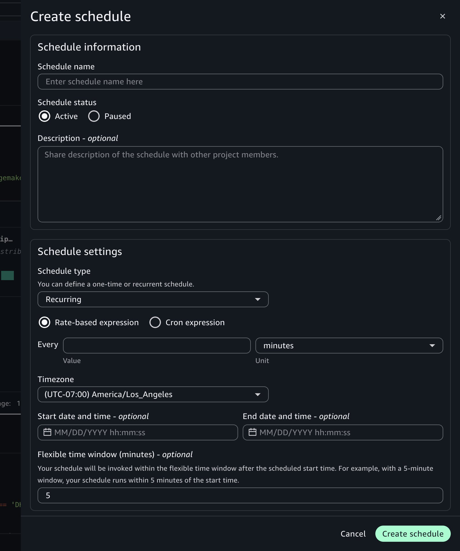
Configure the following settings:

• Schedule name: Enter a descriptive name, such as Daily Shipping Report.
• Schedule type: Choose Recurring for repeated runs or One-time for a single future run.
• Frequency: Define how often the notebook runs using a rate (for example, every one day) or a cron expression. Set the time zone and the start and end dates for the schedule. For example, set the schedule to run every day at 7:00 AM UTC starting tomorrow.
• Flexible time window (optional): The number of minutes after the scheduled start time within which the run can be invoked. For example, with a 5-minute window, the notebook runs within 5 minutes of the start time.
• Advanced settings:
  • Compute Instance: Keep the current settings or override with a different instance type for the asynchronous run to use.
  • Timeout: Set a maximum run duration to help prevent notebooks from running indefinitely. If left blank, it defaults to 60 minutes.

Choose Create.

The schedule appears in the Schedules tab of the activity panel. SageMaker Unified Studio creates an Amazon EventBridge Scheduler schedule for each schedule you configure.

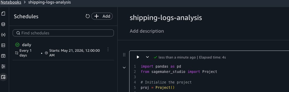
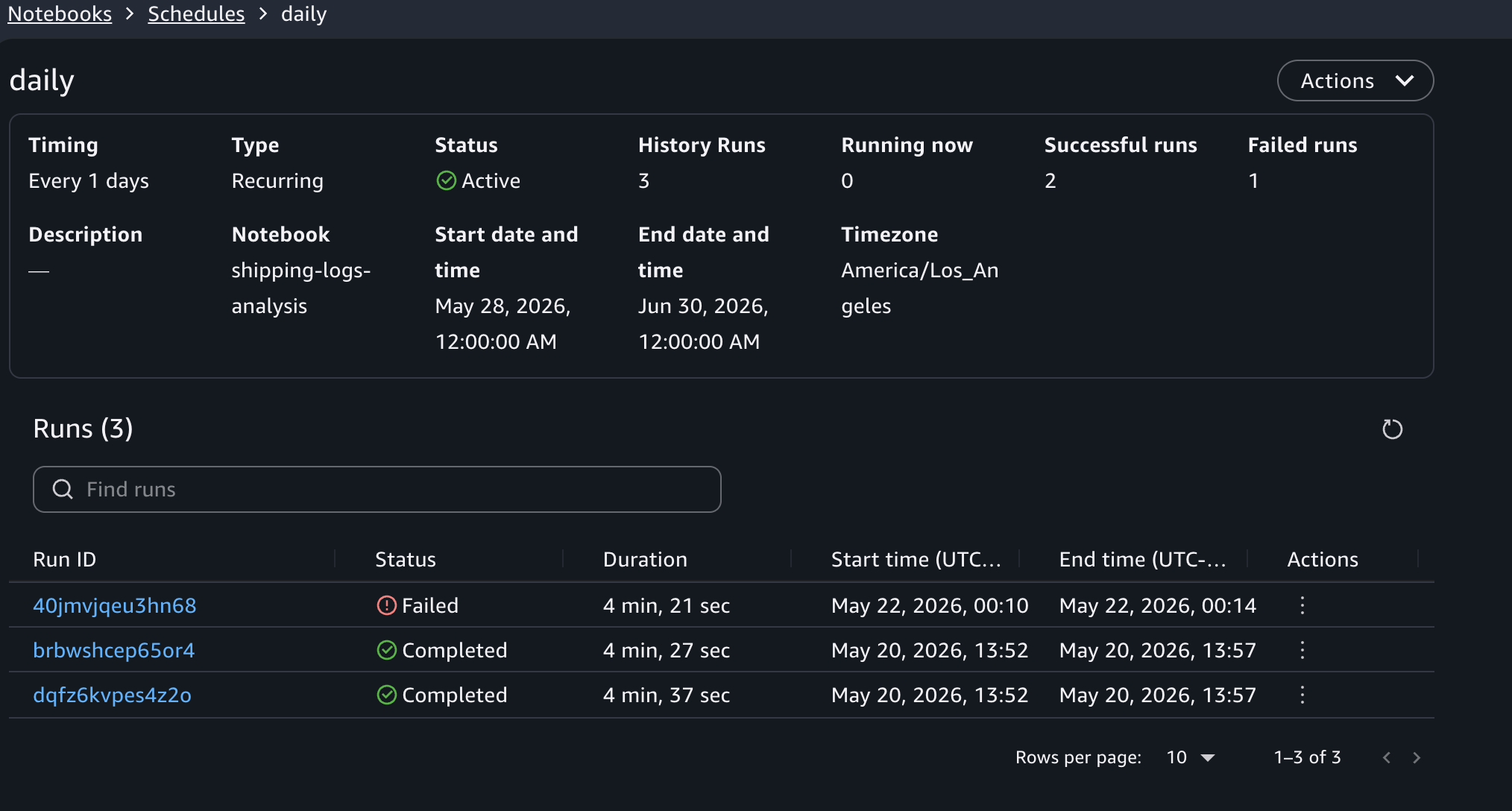
Viewing schedule run history

To view past runs for a schedule, choose the schedule name in the Schedules activity panel. This opens the schedule details view, where you can see the list of runs triggered by that schedule, the duration of each run, and a link to open the notebook output for an individual run.

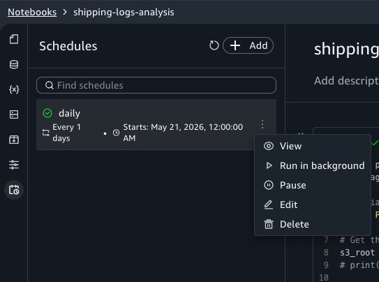
Editing and deleting schedules

To modify a schedule, choose Edit next to it in the Schedules panel. You can change the frequency, instance type, timeout, and other configuration fields. To pause or resume a schedule, choose Pause or Resume from the same menu. To remove a schedule, choose Delete from that menu. Deleting a schedule stops future runs but preserves historical run outputs in Amazon S3 for auditing purposes.

Parameterizing notebooks

With parameters, you can reuse a single notebook across different inputs without duplicating code. For example, you can run the same shipping performance report for each carrier by passing a different carrier name to each run.

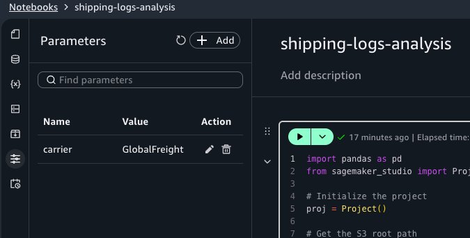
Defining parameters

Open the Parameters activity panel and choose Add. Set the parameter name to carrier and the default value to GlobalFreight.

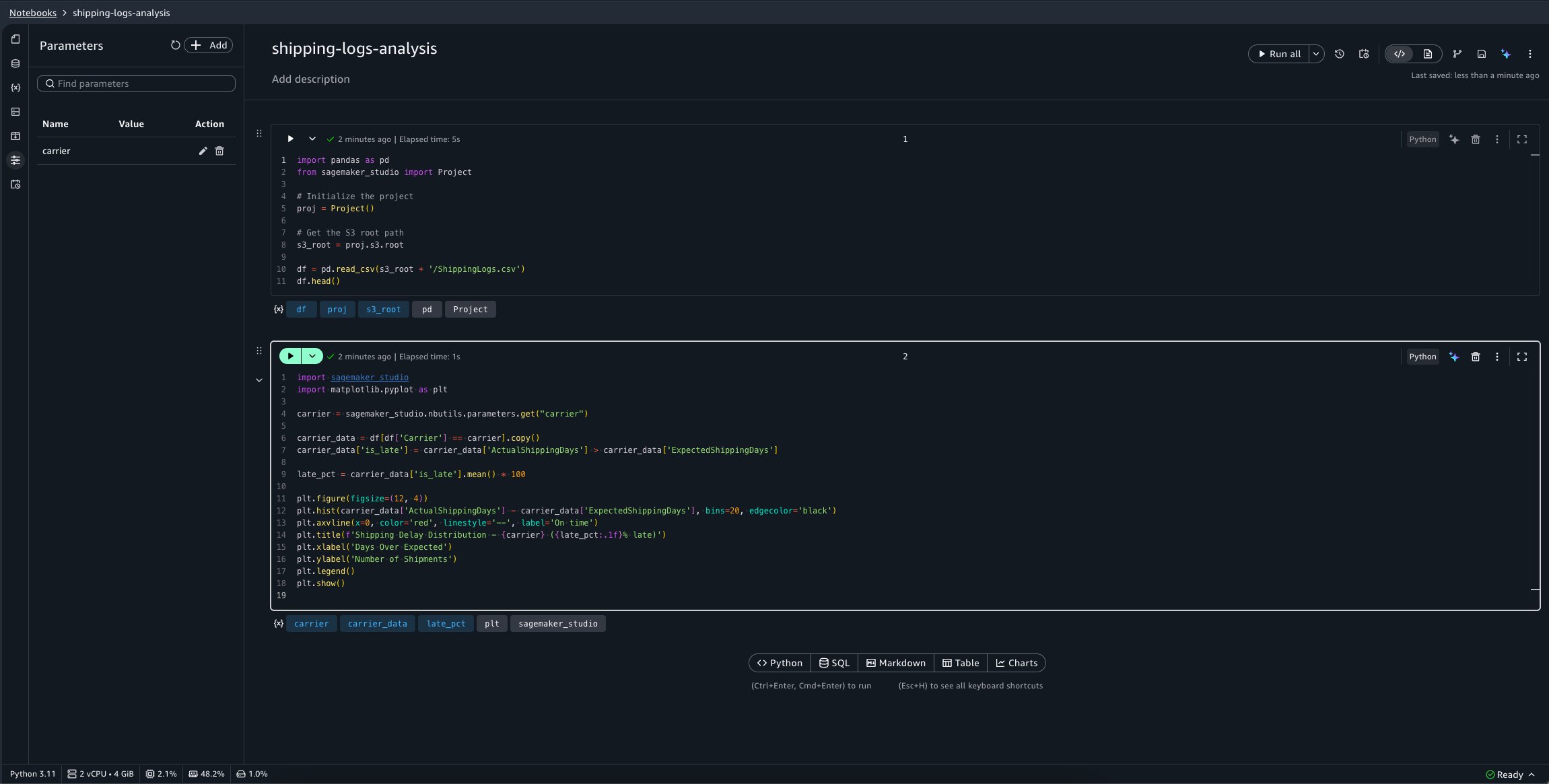
Using parameters in code

In your notebook, replace the second cell with the following code. This retrieves the carrier parameter value using the SageMaker Unified Studio Python SDK instead of the hardcoded value:

import sagemaker_studio
import matplotlib.pyplot as plt

carrier = sagemaker_studio.nbutils.parameters.get("carrier")

carrier_data = df[df['Carrier'] == carrier].copy()
carrier_data['is_late'] = carrier_data['ActualShippingDays'] > carrier_data['ExpectedShippingDays']
late_pct = carrier_data['is_late'].mean() * 100

plt.figure(figsize=(12, 4))
plt.hist(carrier_data['ActualShippingDays'] - carrier_data['ExpectedShippingDays'], bins=20, edgecolor='black')
plt.axvline(x=0, color='red', linestyle='--', label='On time')
plt.title(f'Shipping Delay Distribution - {carrier} ({late_pct:.1f}% late)')
plt.xlabel('Days Over Expected')
plt.ylabel('Number of Shipments')
plt.legend()
plt.show()

Creating schedules with different parameter values

Now create three schedules for the same notebook, each targeting a different carrier:

• “daily-shipping-gf” with carrier = GlobalFreight.
• “daily-shipping-mc” with carrier = MicroCarrier.
• “daily-shipping-shipper” with carrier = Shipper.

When you view a historical run, a separate Parameters tab in the run output displays the parameter values that were active for that run.

You can also override parameter values when triggering an on-demand background run. Choose the menu on the Run all button, then choose Run with settings. You can keep the defaults or provide custom values for that run.

Orchestrating with Workflows

To combine notebooks into a multi-step pipeline, such as running a data calculation notebook before the shipping log notebook, you can use the Notebook Operator in the Workflows tool to orchestrate them.

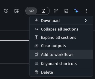
To do this, choose the Add to workflows button under the options menu of the notebook header.

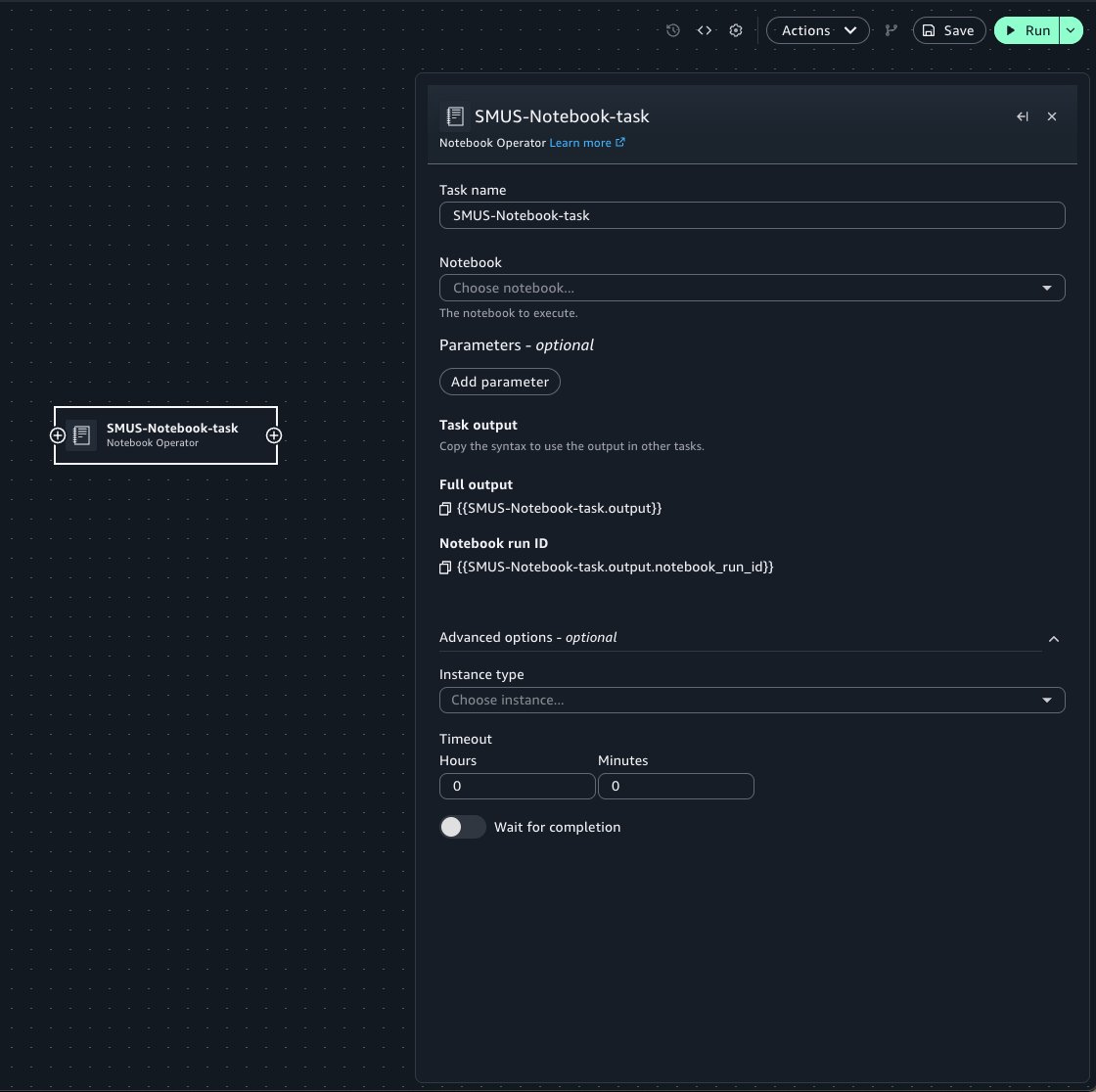
This takes you to the Workflows tool, adding a new Notebook Operator task with prefilled properties from your notebook. When configuring the Operator task:

• Select the target notebook from the notebook menu.
• Use the Parameters widget to pass notebook parameters into the run of the notebook.
• Specify optional arguments such as the compute instance and timeout configuration for the run.

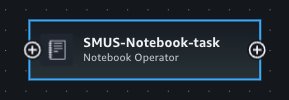
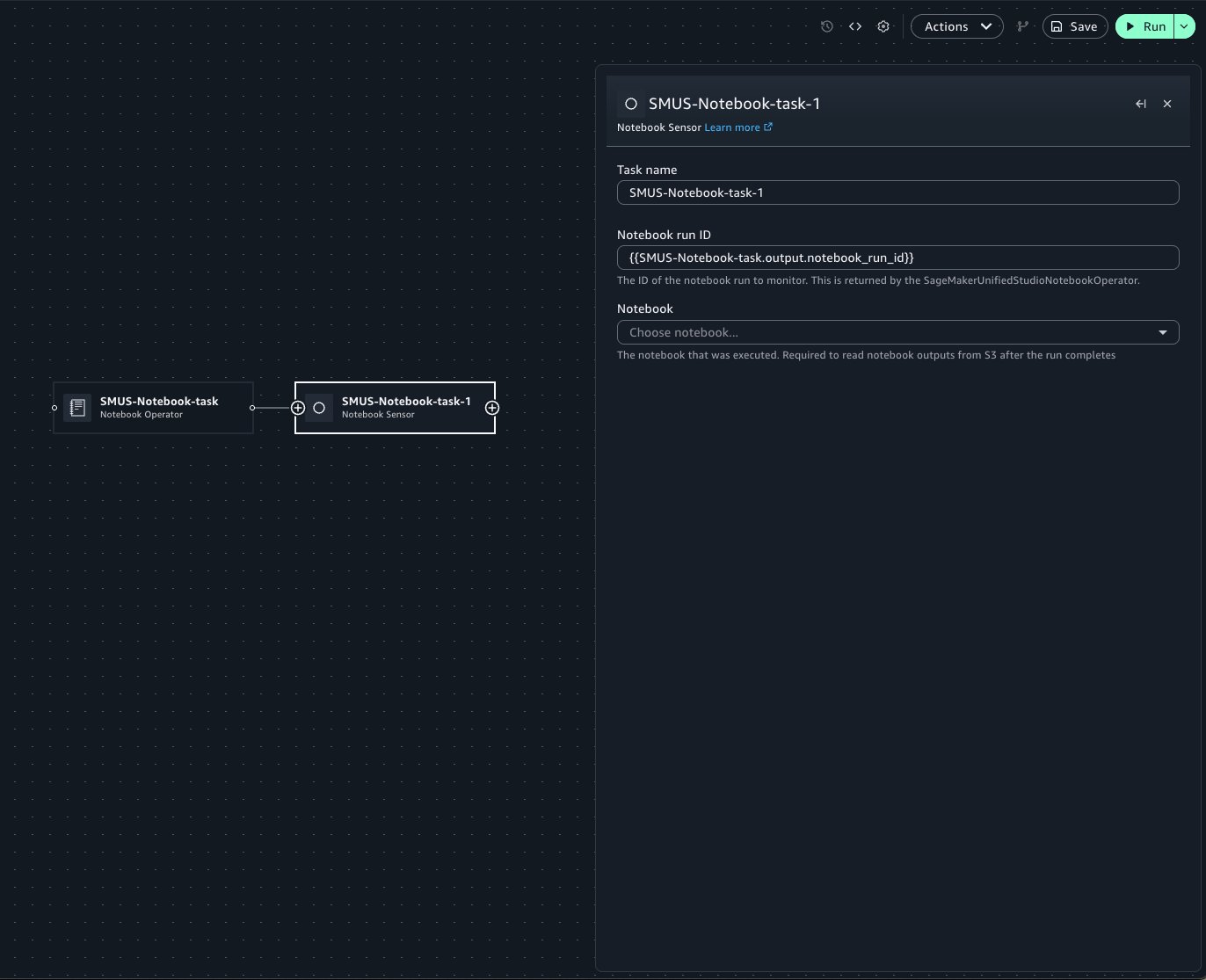
Workflows also supports polling for the status of a notebook run for a particular notebook using Notebook Sensor. In Workflows, you can add a new Sensor task by hovering on the edge of the existing Operator task, where a plus (+) button is displayed.

You can then search for and add the Notebook Sensor to the canvas.

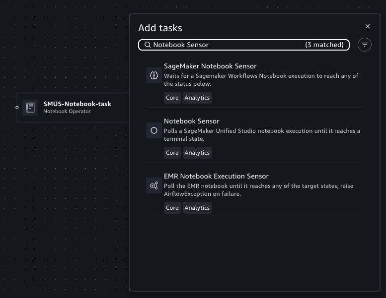
When configuring the Sensor task, specify the notebook run ID within the text field. The Operator’s form field contains Jinja templating to retrieve the notebook run. If the Sensor is used within the same workflow as the Operator, this template can be copied to use within a Sensor to poll the notebook run. Select the target notebook from the notebook menu.

Within Workflows, you can configure notebook runs to emit outputs and use those outputs as inputs for subsequent notebook runs.

Building off of the previous shipping log notebook example, we will pass the carrier parameter from an upstream notebook’s output. Your shipping-logs-analysis notebook should be already set up.

Because the notebook depends on the carrier parameter, you can specify it in the Parameters panel.

Now, define a second notebook, calculate-best-carrier, which performs a calculation to determine our best carrier to use for shipping:

import pandas as pd
from sagemaker_studio import Project

# Initialize the project
proj = Project()

# Get the S3 root path
s3_root = proj.s3.root

df = pd.read_csv(s3_root + '/ShippingLogs.csv')
df.head()

carrier_stats = df.groupby('Carrier').agg(
    total=('OrderID', 'count'),
    late=('OnTimeDelivery', lambda x: (x == 'Late').sum())
).reset_index()
carrier_stats['late_pct'] = carrier_stats['late'] / carrier_stats['total'] * 100

best = carrier_stats.sort_values('late_pct', ascending=True).iloc[0]
best_carrier = best['Carrier']

print("Late % by carrier:")
print(carrier_stats.to_string(index=False))
print(f"\nBest carrier: {best_carrier} ({best['late_pct']:.1f}% late)")

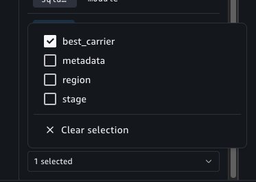
To configure the calculate-best-carrier notebook’s outputs, you can choose the Variables panel. A new selector is available at the bottom of this panel which allows you to select variables to mark as outputs.

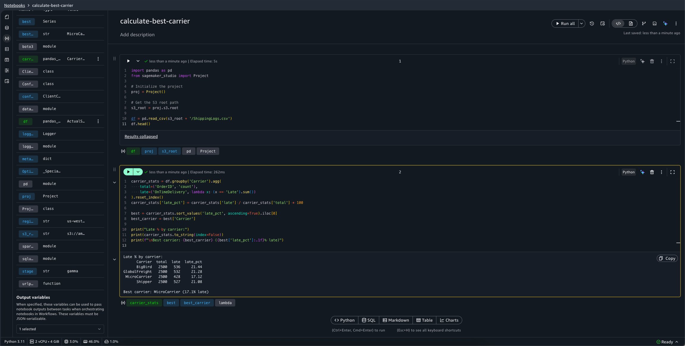
We want this notebook to emit the best_carrier variable.

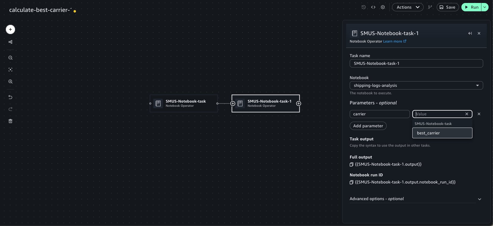
Now, use the Add to workflows button as previously demonstrated to quickly add this notebook within a workflow. Chain a second Notebook Operator that points to our shipping-logs-analysis notebook. Because we specified a parameter dependency on carrier for this notebook, it’s available as an option in the Parameters widget menu.

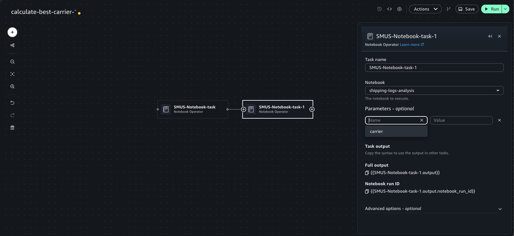
When they’re chained, the notebook tasks detect the outputs set in upstream notebook runs. These outputs can be selected as keys within the Parameters widget of the Operator to pass into the run. This can be done recursively for an arbitrary number of Operator tasks. We can select the emitted best_carrier output from the calculate-best-carrier notebook.

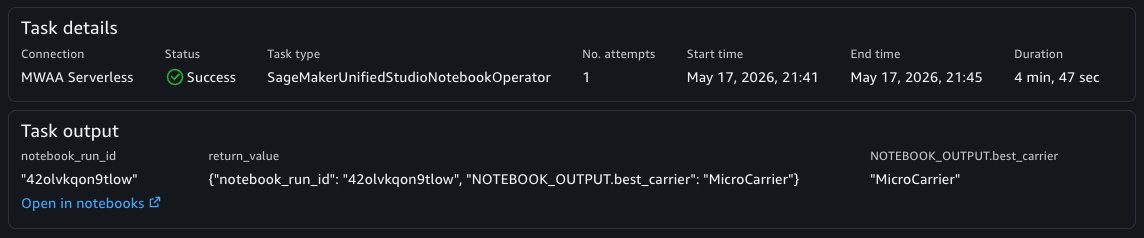
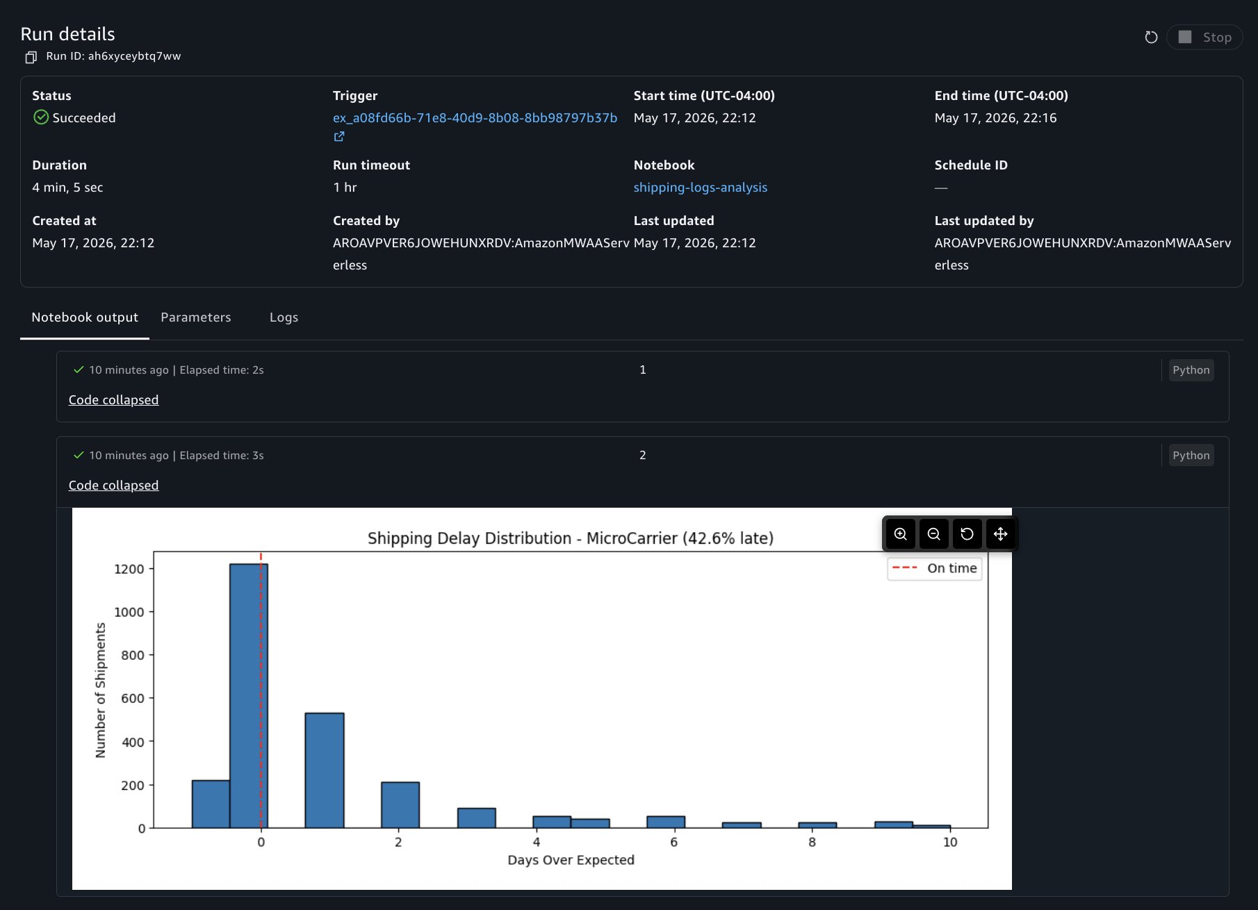
You can now choose the Save button on the top left of the visual canvas and the Run button to start the workflow. When the workflow is completed, the specified notebook outputs are available in the Task Output panel and the notebook run result can be viewed in the Notebooks tool.

In a similar manner, the Notebook Sensor will also emit the notebook outputs from a particular notebook’s run which can be used within other tasks. This is useful when you want to retrieve outputs from a notebook run in another workflow.

Debugging a failed run with AI assistance

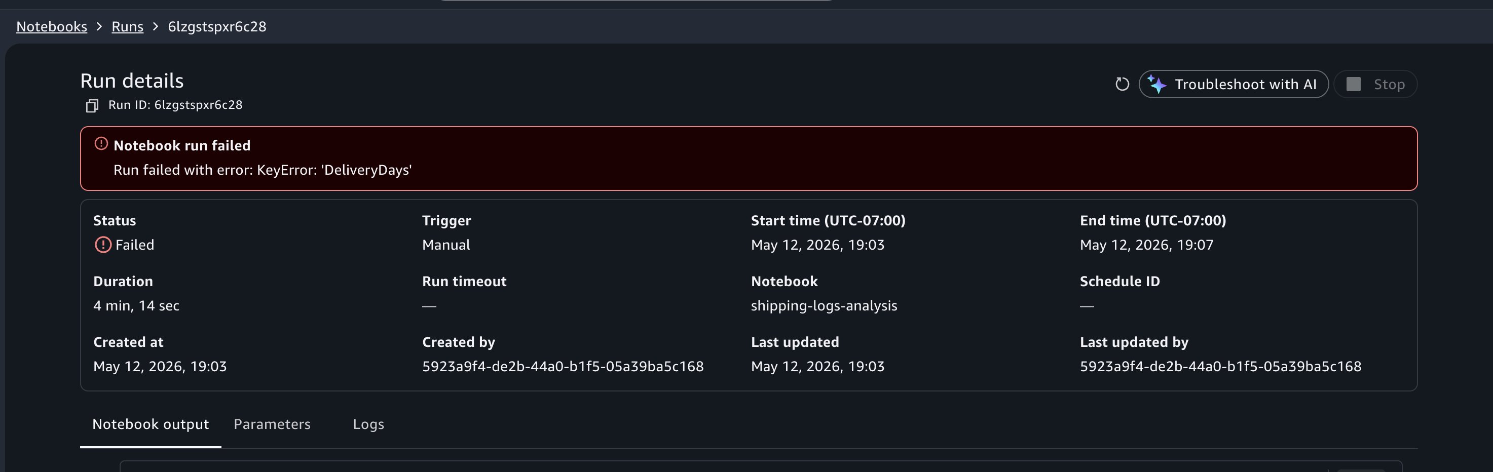
When viewing your past runs, you notice that a run from earlier today has a Failed status. Choose the failed run to open the notebook output in read-only mode.

In this example, suppose you incorrectly referred to column name ActualShippingDays as DeliveryDays. The run would fail with a KeyError: 'DeliveryDays' in the cell that computes late deliveries.

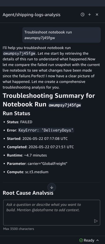
At the top of the failed run output, choose Troubleshoot with AI. Choosing the Troubleshoot with AI button lands you in the notebook with the Agent chat panel open.

The data agent analyzes the cell outputs, identifies the cell that errored, explains the root cause, and suggests a fix. In this case, it identifies that the column DeliveryDays doesn’t exist in the dataframe and suggests updating the code reference. You can review the change, then verify the fix by choosing Run in background from the Run all menu to trigger a test run before the next scheduled run.

Note: You can also use the Data Agent to create schedules and start notebook runs using natural language, without having to navigate.

Cleaning up

To avoid incurring future charges, delete the resources that you created in this walkthrough:

• Delete any schedules that you created from the Schedules panel in your notebook.
• Delete test notebooks if you don’t need them.
• Navigate to the Workflows page and delete any workflows that you created during this walkthrough.
• Your project’s Amazon S3 storage retains historical run outputs until you manually remove them.

Conclusion

In this post, we showed how to run notebooks in the background in Amazon SageMaker Unified Studio using background runs, schedules, parameterization, workflow orchestration, and AI-assisted debugging. Using a shipping logistics dataset, we demonstrated how a single notebook can be parameterized to generate performance reports for different carriers on independent schedules, all without duplicating code or managing extensive infrastructure.

To get started, open a notebook in your SageMaker Unified Studio project, choose the menu on the Run all button in the notebook header, and choose Run in background. For more advanced use cases, explore workflows in Amazon SageMaker Unified Studio to build multi-step data pipelines, or review the Amazon SageMaker Unified Studio User Guide for additional configuration options.

Learn more:

• Amazon SageMaker Unified Studio User Guide.
• Notebooks in SageMaker Unified Studio.
• Manage compute environments.
• Amazon SageMaker Unified Studio pricing.

If you have feedback or questions, reach out on AWS re:Post for Amazon SageMaker Unified Studio.

About the authors