Tag Archives: Amazon SageMaker Unified Studio

Discover and govern Snowflake data using SageMaker Unified Studio

Post Syndicated from Marco Duarte original https://aws.amazon.com/blogs/big-data/discover-and-govern-snowflake-data-using-sagemaker-unified-studio/

Many organizations operate in hybrid data environments where critical assets live in Snowflake while analytics workloads run on AWS, which can create governance gaps, discovery friction, and duplicated efforts when the two aren’t connected.

With Amazon SageMaker Unified Studio, you can govern data across Snowflake and AWS through its integrated catalog and AWS Glue Data Quality, a capability of AWS Glue. You connect directly to Snowflake tables without moving data, apply quality rules using AWS Glue Visual ETL, and publish validated assets to Amazon SageMaker Catalog, maintaining consistent governance across your entire distributed data estate.

Without this integration, cataloging Snowflake data requires building extraction pipelines, often taking days. With SageMaker Unified Studio connected to Snowflake, you can query, catalog, and validate the quality of federated data in 5–15 minutes. No data replication or custom ETL code required.

In this post, we show you how to connect Snowflake to Amazon SageMaker Unified Studio, register data assets in Amazon SageMaker Catalog, configure data quality validation using AWS Glue Visual ETL, and publish assets for unified collaboration. By following these steps, you enrich federated assets with data quality scores so that consumers across your organization can discover and trust the data, all while keeping it in Snowflake.

Solution overview

This solution integrates Snowflake with Amazon SageMaker Unified Studio for centralized data cataloging and quality validation.

The architecture uses an AWS Glue connection to federate the Snowflake catalog into Amazon SageMaker Unified Studio. Tables become available in the project catalog without complex storage configurations. You can query data directly using SQL analytics, publish datasets to Amazon SageMaker Catalog for organization-wide discovery, and apply data quality rules through AWS Glue Visual ETL pipelines.

The workflow consists of the following steps:

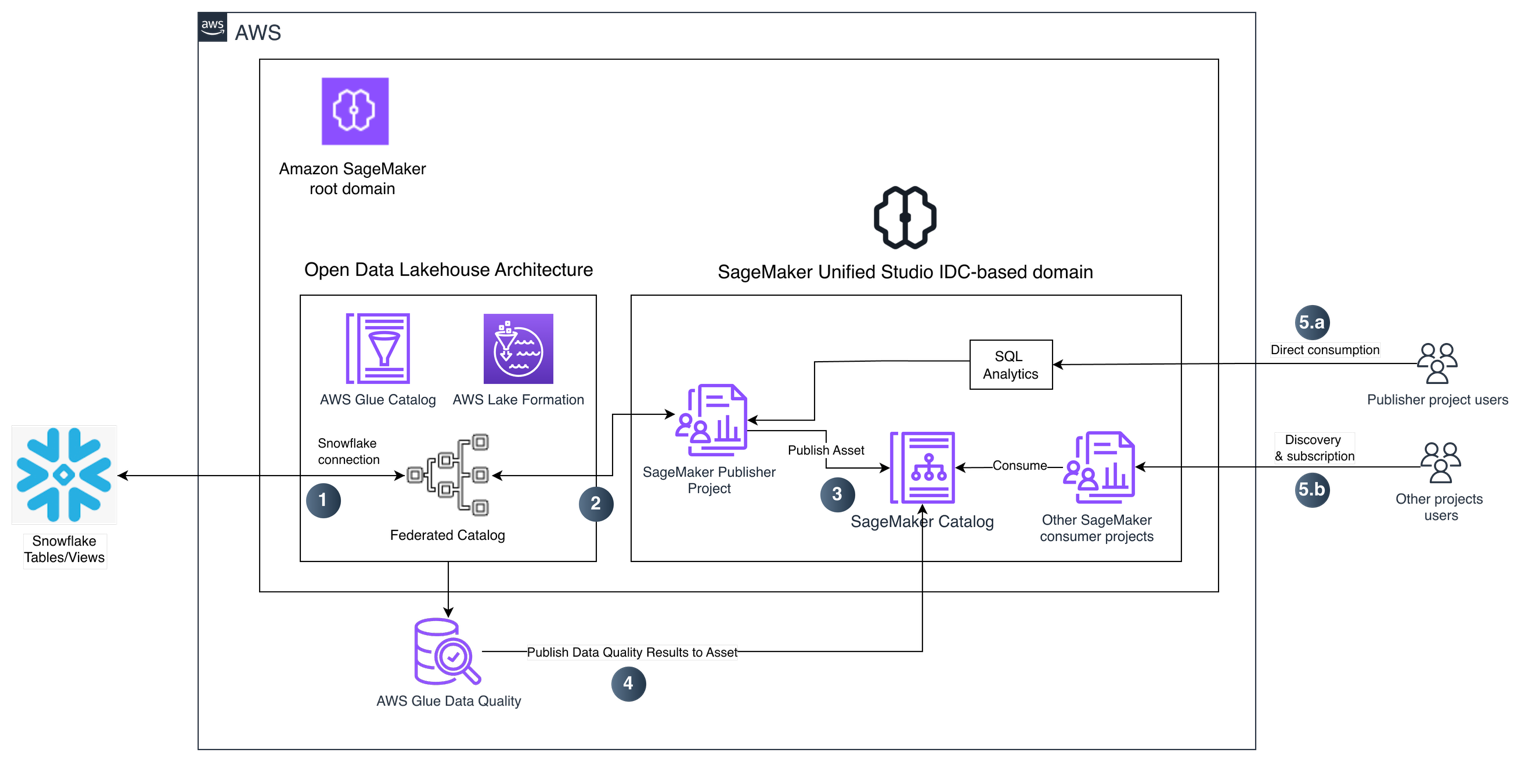
Architecture diagram: Snowflake federated into SageMaker Unified Studio through AWS Glue, with data quality validation and publishing to SageMaker Catalog

Figure 1: Architecture for federating Snowflake into SageMaker Unified Studio and validating data quality

  1. Snowflake connection creation on Amazon SageMaker Unified Studio — Amazon SageMaker Unified Studio uses an AWS Glue connection to federate Snowflake tables and views into its open data lakehouse architecture. The federated catalog entry is registered in AWS Glue Data Catalog and governed by AWS Lake Formation for centralized access control, without moving data out of Snowflake.
  2. Federate Snowflake tables into the Amazon SageMaker publisher project — The Amazon SageMaker publisher project discovers the federated Snowflake tables through the AWS Glue Data Catalog integration.
  3. Publish the dataset to Amazon SageMaker Catalog — The publisher project publishes the dataset as a governed asset to the Amazon SageMaker Catalog, making it discoverable for data consumers across the organization.
  4. Validate data quality — AWS Glue Data Quality runs validation rules against the federated Snowflake data and publishes the data quality results directly to the corresponding asset in Amazon SageMaker Catalog.
  5. Consume data — Users access Snowflake data through two paths:
    1. Publisher project users — Query data with SQL Analytics — Users in the publisher project can query the Snowflake data directly using Amazon SageMaker Unified Studio SQL Analytics for interactive exploration and analysis, without copying or moving data.
    2. Consumer project users — Discovery and subscription through SageMaker Catalog — Other Amazon SageMaker consumer projects discover the published asset in the Amazon SageMaker Catalog, subscribe to it, and consume the data for their analytics and machine learning workloads.

Prerequisites

To follow along, you need:

  • An active Snowflake account with administrator access.
  • Tables or views created within a schema inside a Snowflake database.
  • An Amazon SageMaker Unified Studio and project created.
  • An Amazon Simple Storage Service (Amazon S3) bucket for AWS Glue assets.
  • Appropriate AWS Identity and Access Management (IAM) permissions configured (Amazon SageMaker Catalog is built on Amazon DataZone, so the IAM actions use the datazone: prefix.)

Your AWS Glue job execution role requires specific permissions to interact with Amazon SageMaker Catalog.

Required IAM policies for the AWS Glue job role

1. Amazon SageMaker Catalog search and listing permissions: Attach a policy that allows the AWS Glue job to search and list assets in Amazon SageMaker Catalog.

{
  "Version": "2012-10-17",
  "Statement": [
    {
      "Effect": "Allow",
      "Action": [
        "datazone:SearchListings",
        "datazone:GetListing",
        "datazone:ListDomains",
        "datazone:GetDomain"
      ],
      "Resource": "arn:aws:datazone:<REGION>:<ACCOUNT_ID>:domain/<DOMAIN_ID>"
    }
  ]
}

2. Amazon SageMaker Catalog time series data posting permissions: Add permissions to post data quality metrics:

{
  "Version": "2012-10-17",
  "Statement": [
    {
      "Effect": "Allow",
      "Action": [
        "datazone:PostTimeSeriesDataPoints",
        "datazone:GetAsset",
        "datazone:ListAssetRevisions"
      ],
      "Resource": "arn:aws:datazone:<REGION>:<ACCOUNT_ID>:domain/<DOMAIN_ID>"
    }
  ]
}

Configure the AWS Glue job role as an Amazon SageMaker domain user

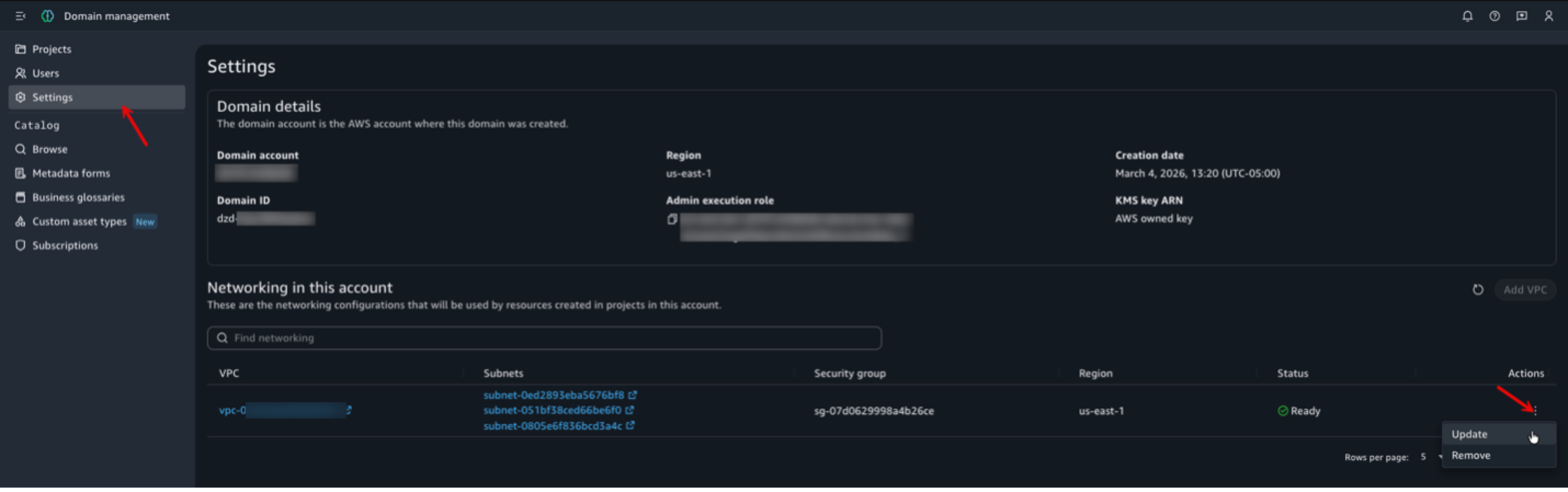
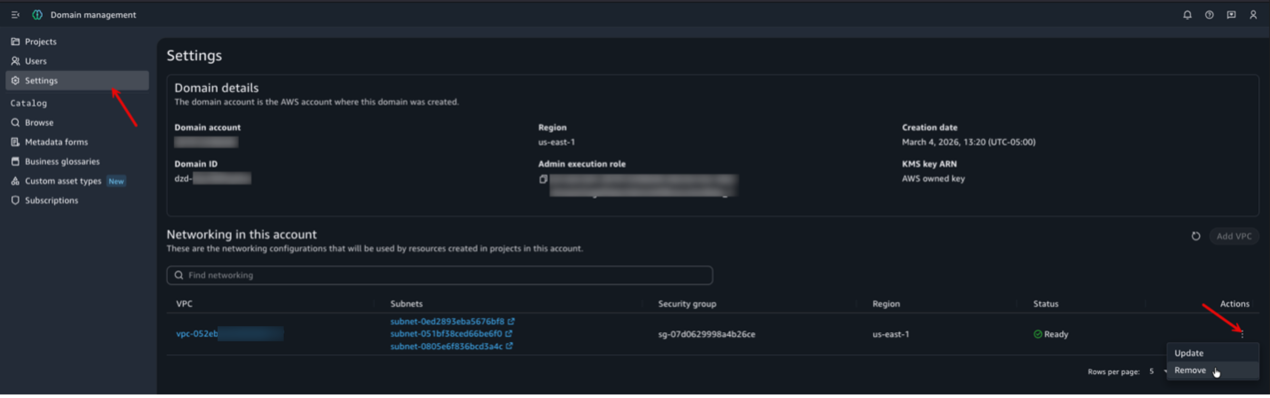
Configure the IAM role used by your AWS Glue job as a domain user. In the Amazon SageMaker console, navigate to your domain, choose Access management, and add the AWS Glue job execution IAM role as a domain user.

Project-level permissions

Add the AWS Glue job execution role as a project member with Owner permissions. Navigate to your project, go to Project settings > Members, and add the role.

For more information about IAM roles for AWS Glue, see the AWS Glue security documentation. For Amazon SageMaker Unified Studio permissions, refer to the Amazon SageMaker Unified Studio administrator guide.

Querying Snowflake datasets from Amazon SageMaker Unified Studio

The following sections walk you through connecting Snowflake to Amazon SageMaker Unified Studio and running data quality validation with results displayed in Amazon SageMaker Catalog.

Identifying information in Snowflake

First, gather your Snowflake connection details. You need a Snowflake account with tables or views created at the schema level within a database.

To obtain Snowflake connection information:

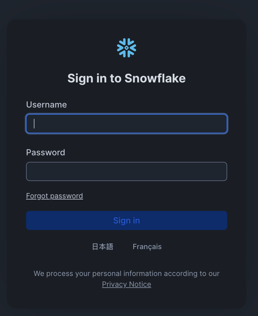
  1. Navigate to your Snowflake environment and sign in with administrator credentials.

    Snowflake sign-in screen for administrator credentials
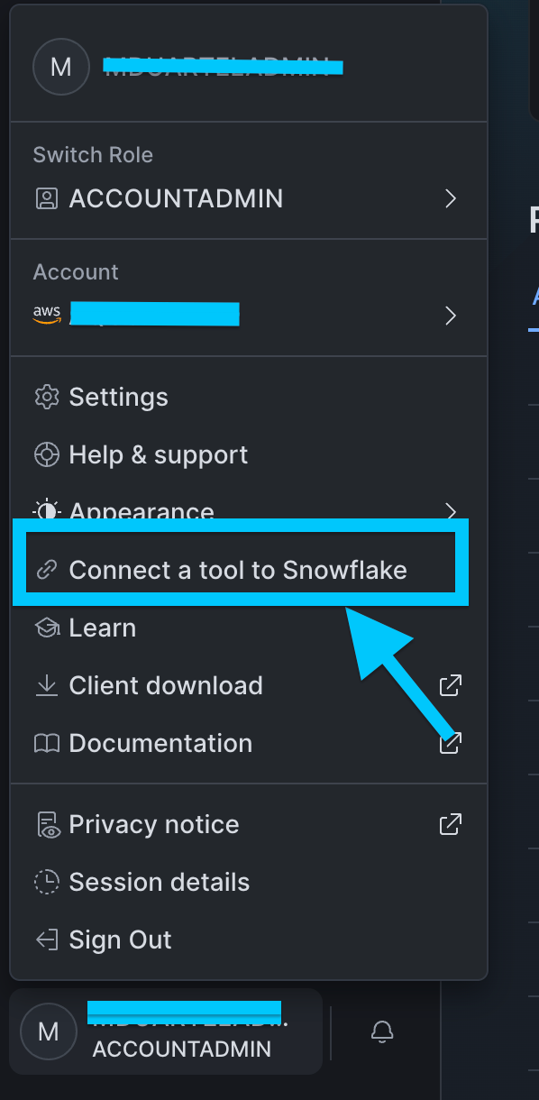
  2. Choose your user account and choose Connect a tool to Snowflake.

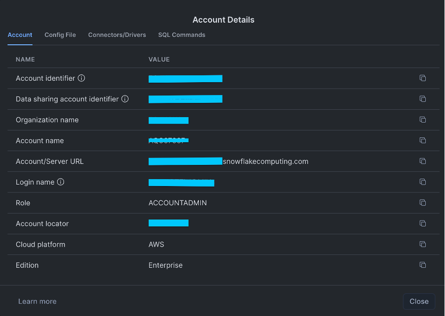
  3. Note the Account/Server URL displayed on the screen.
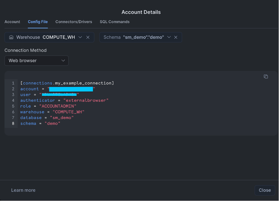
  4. Choose the Config File tab, select values for Warehouse, Database, and Schema, and copy these values for use in the next section.

Creating the connection in Amazon SageMaker Unified Studio

The Add Connection feature stores Snowflake connectivity details including credentials, server, and database information. Amazon SageMaker Unified Studio uses this connection to federate the Snowflake catalog through AWS Glue, so you can query data within minutes of setup.

You need an Amazon SageMaker Unified Studio domain and a project, which acts as a data producer project.

To create the Snowflake connection:

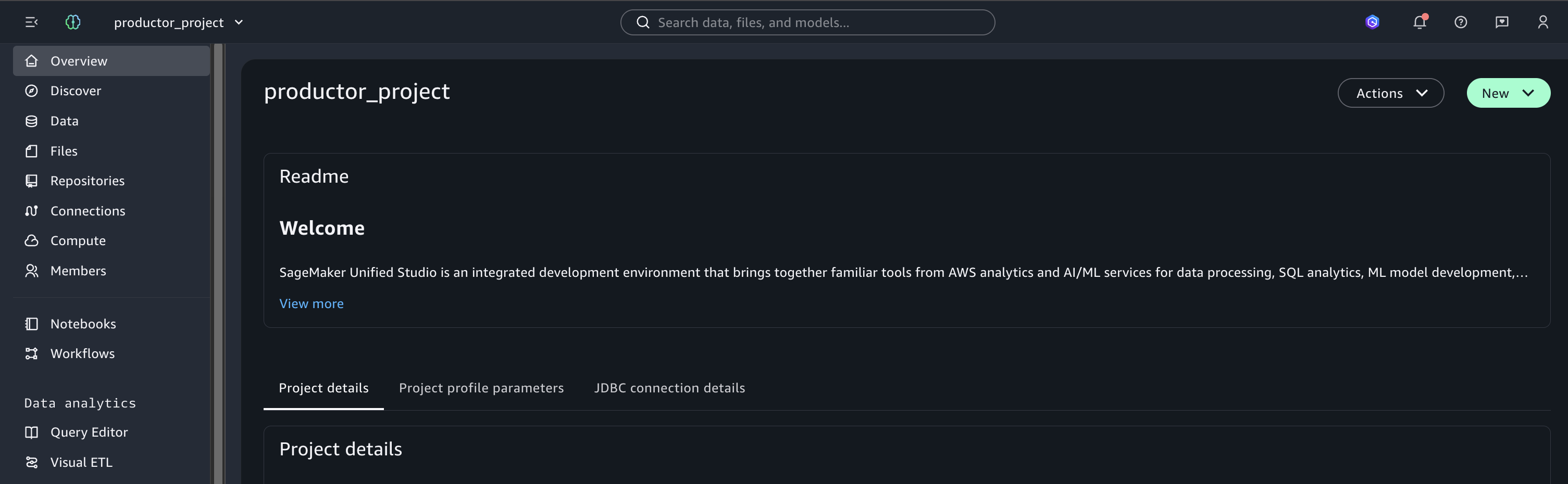
  1. In your Amazon SageMaker Unified Studio project, go to Overview.

    SageMaker Unified Studio project Overview page
  2. Choose Data.

    Data option in the SageMaker Unified Studio project navigation
  3. Choose + Add, then choose Add Connection.

    Add menu in SageMaker Unified Studio with the Add Connection option
    Add Connection panel in SageMaker Unified Studio
  4. Choose Next.
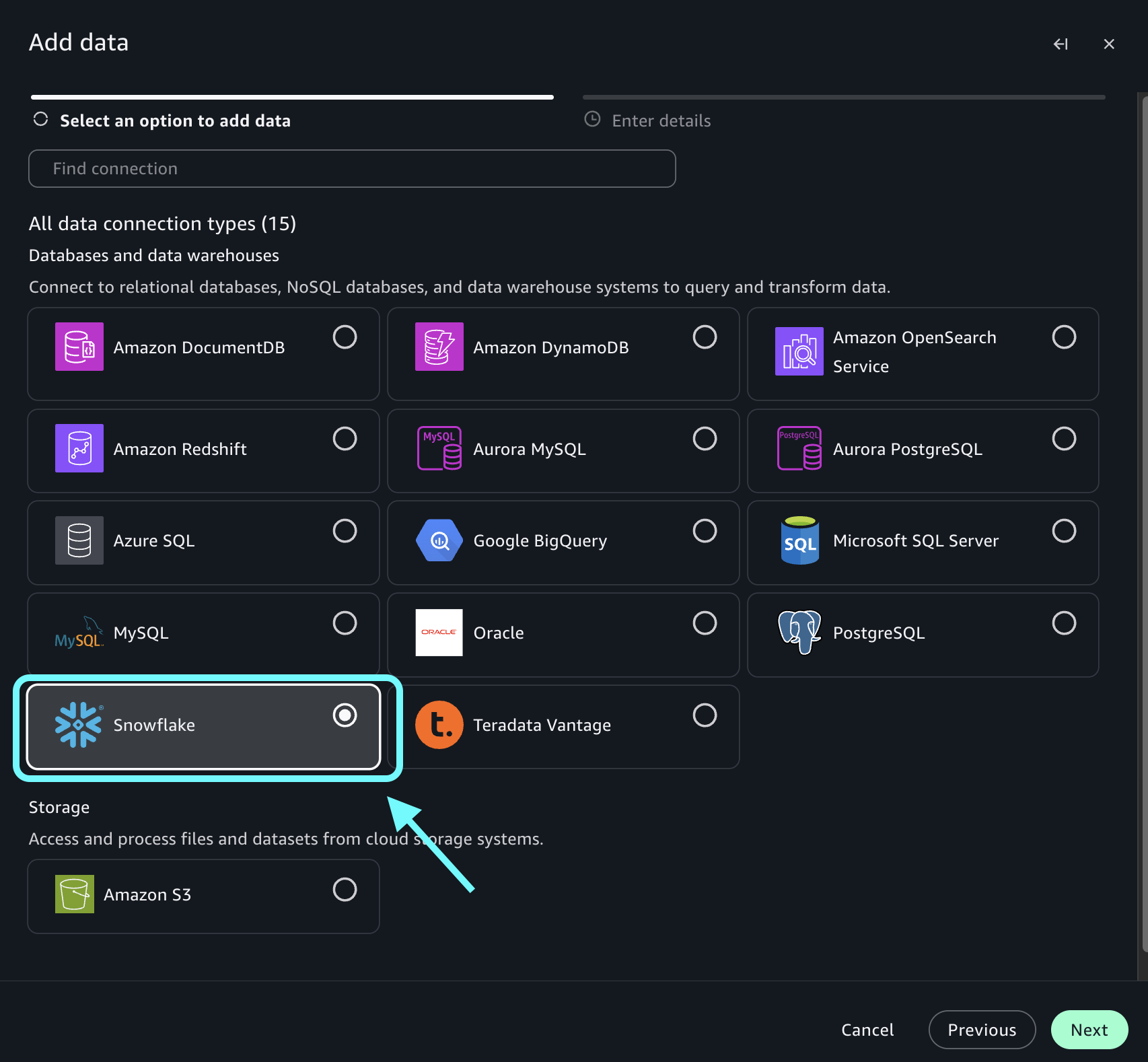
  5. Select Snowflake and choose Next.

    Connection type selection showing Snowflake in SageMaker Unified Studio
  6. Complete the connection details:
    • Name: snowflake-connection.
    • Description (Optional): Enter a description for your connection.
    • Host: Your Snowflake account URL (for example, XXXXXXXXX-XXX000000.snowflakecomputing.com).
    • Port: 443.
    • Database: Your database name (for example, sm_demo).
    • Warehouse: Your warehouse name (for example, COMPUTE_WH).
    • Schema: Your schema name (for example, demo).
    • Additional Properties:
      • Register in AWS Glue Data Catalog: Turn on checkbox.
      • Case conflict handling: Select the option based on Snowflake naming syntax.
    • Authentication:
      • Username: Your Snowflake username.
      • Password: Your Snowflake password.
    Snowflake connection details form with name, host, port, database, warehouse, and schema fields
    Connection form showing authentication and AWS Glue Data Catalog registration options
  7. Choose Add Data.

After creating the connection, wait a few minutes for the federated connection to be established. Search within Amazon SageMaker Unified Studio for the database and created objects.

Federated Snowflake database and objects appearing in SageMaker Unified Studio search

Federated Snowflake tables registered in the AWS Glue Data Catalog

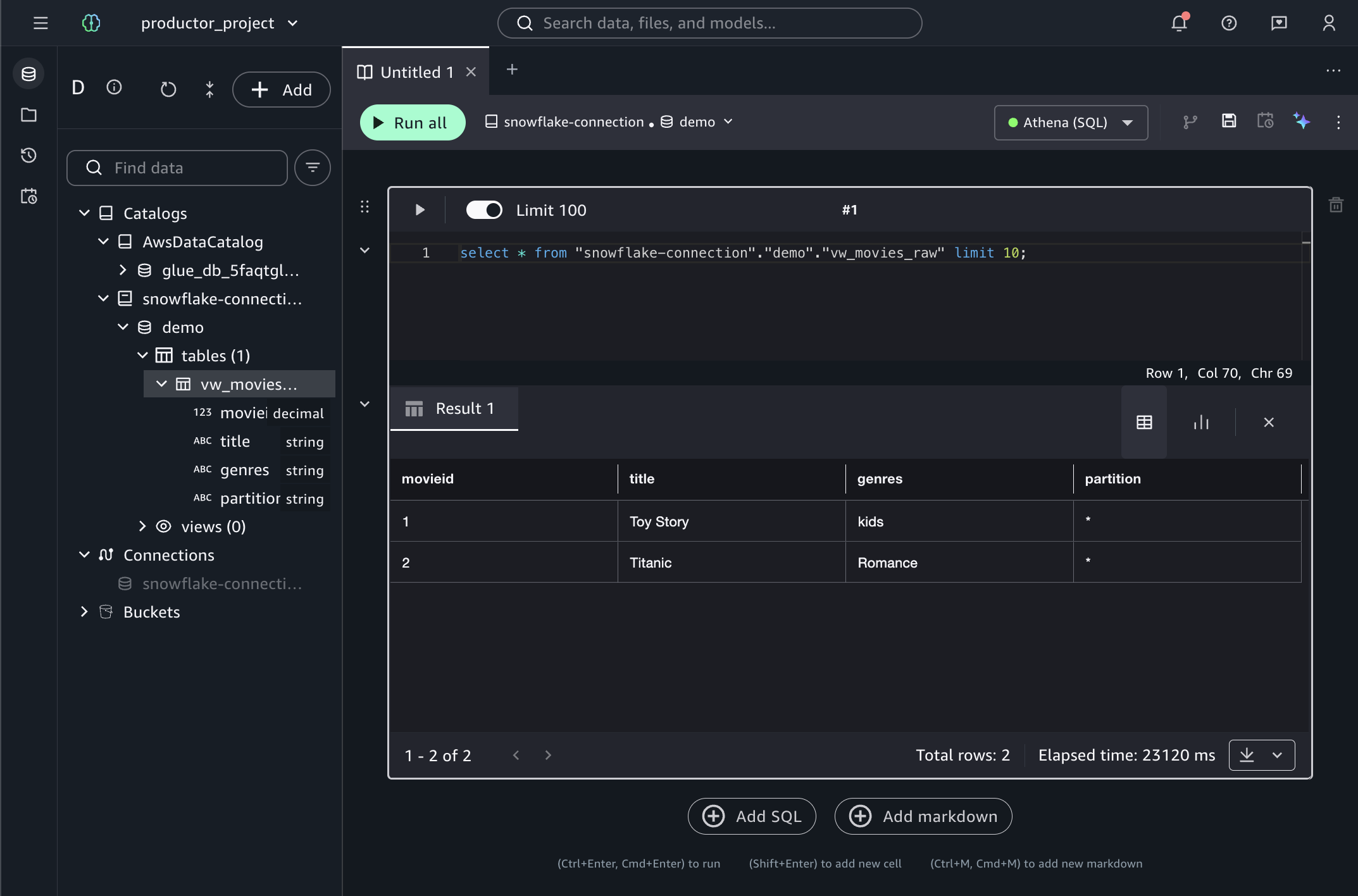
With the Snowflake connection established and the federated tables registered in AWS Glue Catalog, you’re now ready to query Snowflake data directly from Amazon SageMaker Unified Studio, without moving or replicating any data.

Query results from a federated Snowflake table in the SageMaker Unified Studio query editor

How federated queries work

When you run a query in the Amazon SageMaker Unified Studio query editor against a federated Snowflake table, Amazon Athena runs the request. Athena is the underlying query engine integrated into Amazon SageMaker Unified Studio. Athena reads the table definition from AWS Glue Catalog, connects to Snowflake through the established connection, and pushes the query down for execution. Athena returns results directly to the query editor while Snowflake processes the data in place, and only the query results travel across the connection. Amazon SageMaker Unified Studio doesn’t copy data to S3 or any intermediate storage.

After you’ve validated that queries return the expected results, the next step is to publish this dataset to Amazon SageMaker Catalog, making it discoverable and shareable across your organization.

Publishing Snowflake datasets to the SageMaker Catalog

Now that your Snowflake connection is configured, you can publish your datasets to the Amazon SageMaker Catalog, making them discoverable and shareable across your organization.

Creating data assets in SageMaker Catalog

Data assets in Amazon SageMaker Catalog are the cataloged representation of your data resources. They help teams discover, govern, and share data across your organization.

In this section, you create a data asset associated with a Snowflake table. This process transforms a technical Snowflake table into a cataloged resource enriched with business metadata.

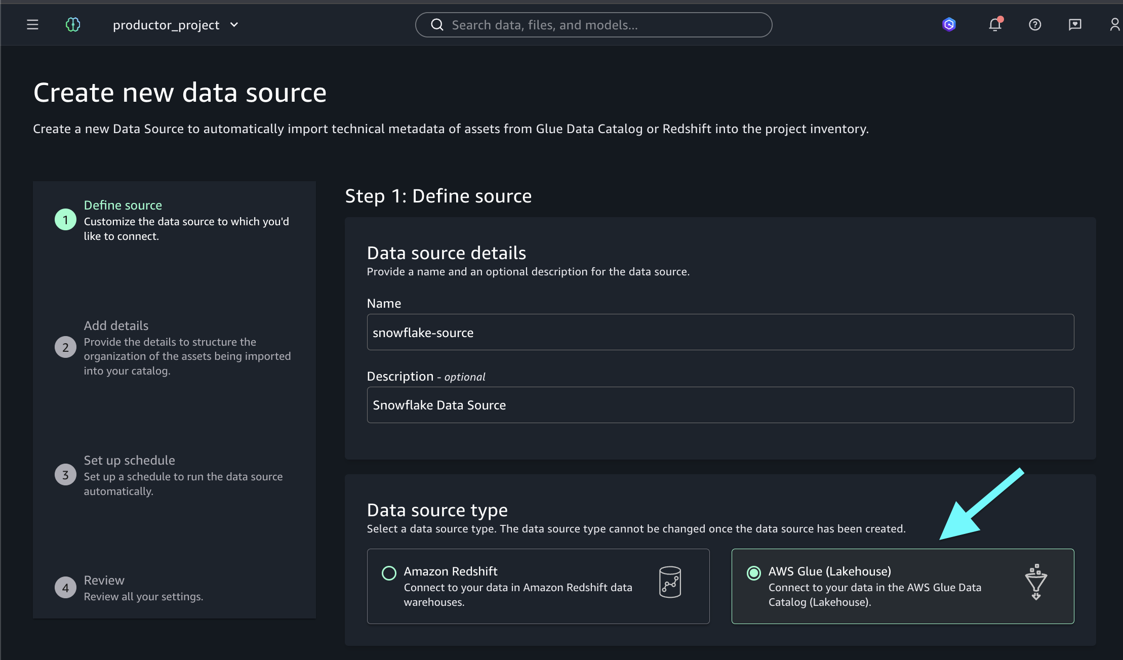
To create a data source:

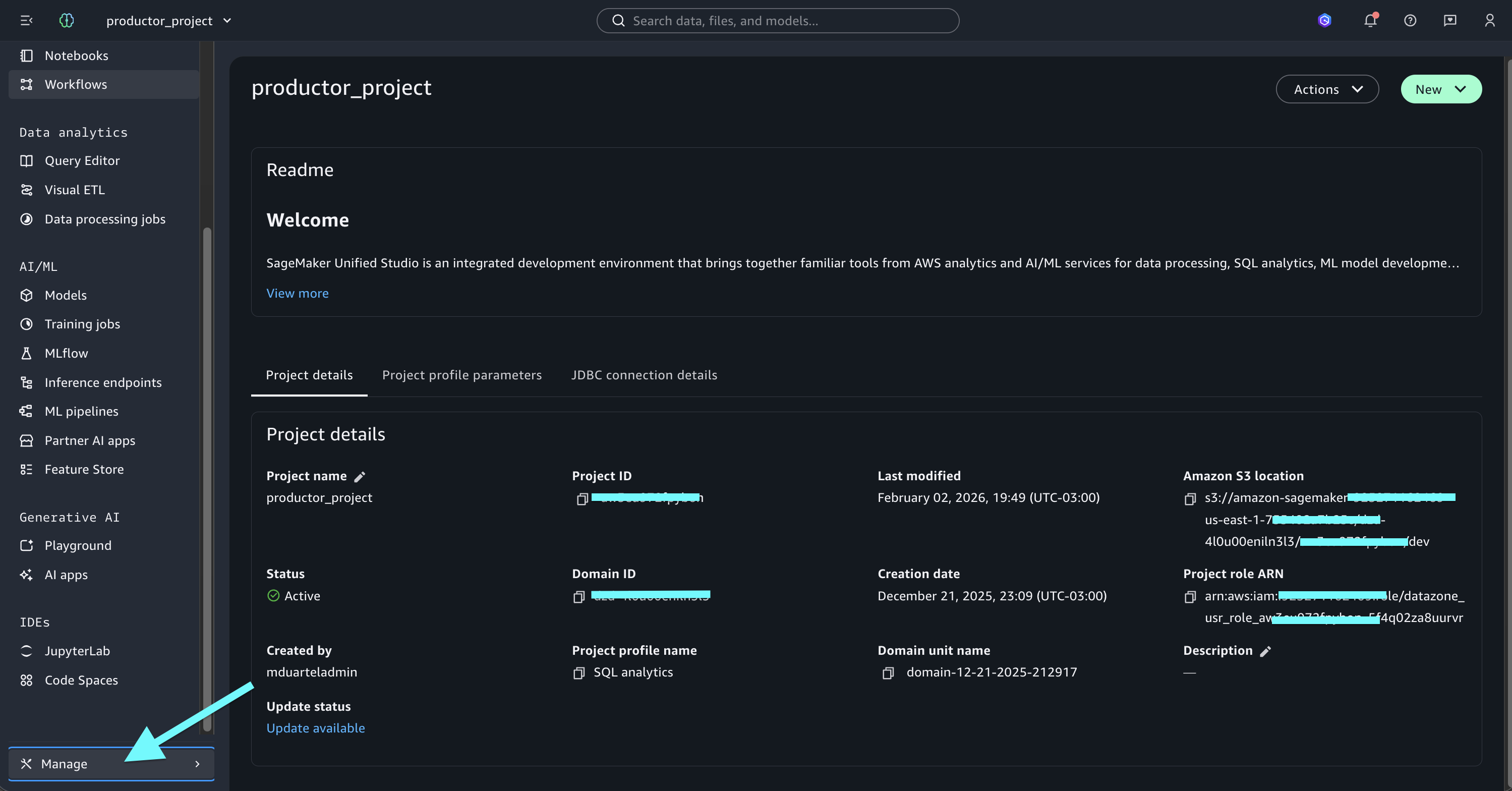
  1. In your Amazon SageMaker Unified Studio project, go to Manage.

    Manage tab in the SageMaker Unified Studio project
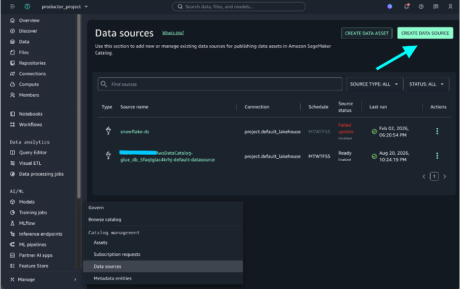
  2. Choose Data Sources.
  3. Choose Create Data Source.

  4. Select the AWS Glue option.

    Data source type selection showing the AWS Glue option
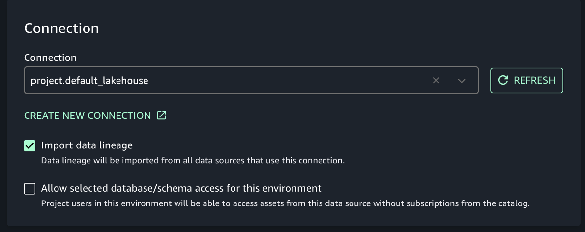
  5. Turn on the Import data lineage checkbox and select the connection: project.default_lakehouse.

    Data source configuration with Import data lineage and the project.default_lakehouse connection selected
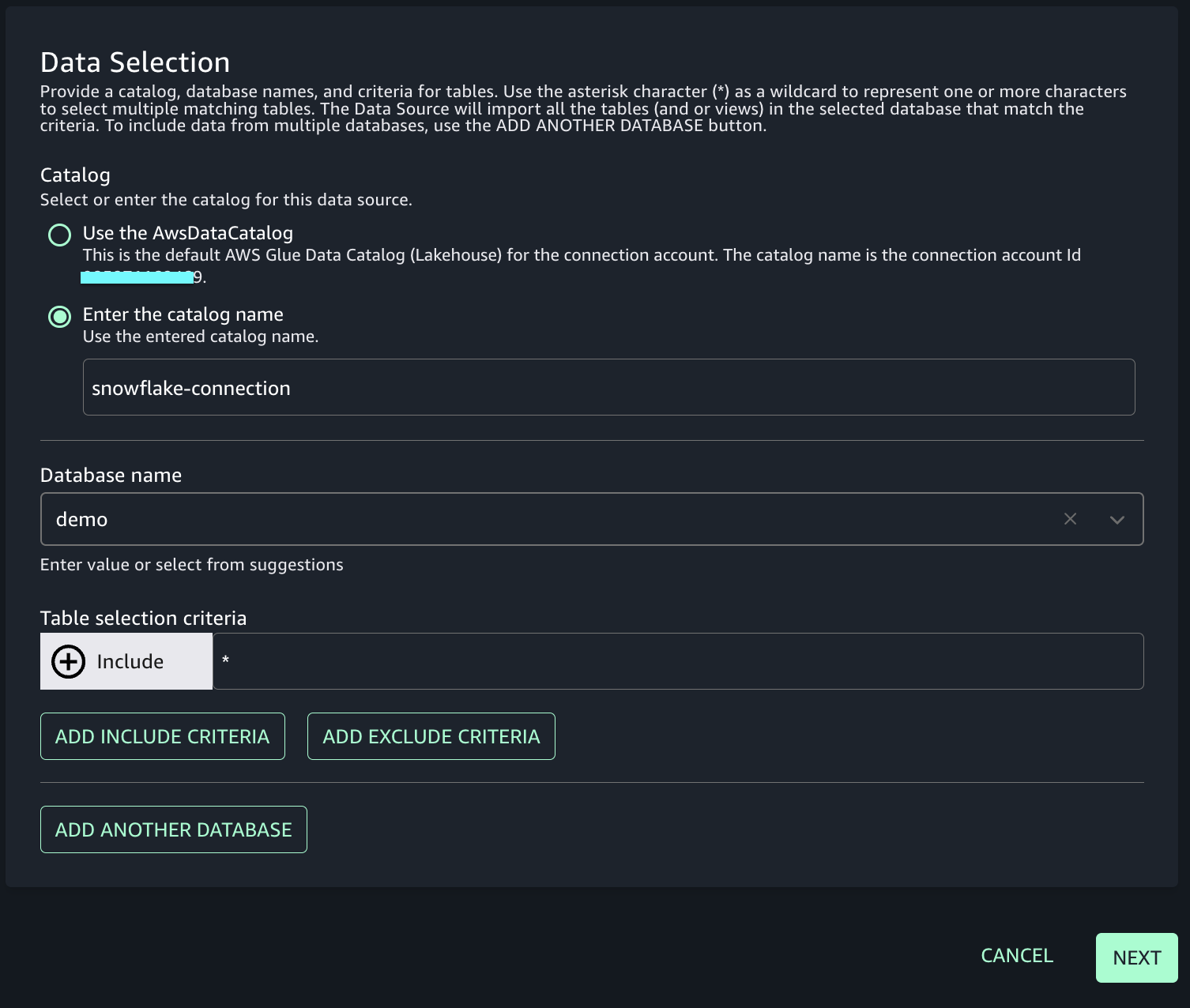
  6. Complete the form and choose Next:
    • Catalog: Select Enter the catalog name and enter snowflake-connection.
    • Database name: Enter your database name (for example, movies).
    • Table selection criteria: Enter * for all tables in the database, or enter a specific table name.
    Data source form showing catalog name, database name, and table selection criteria
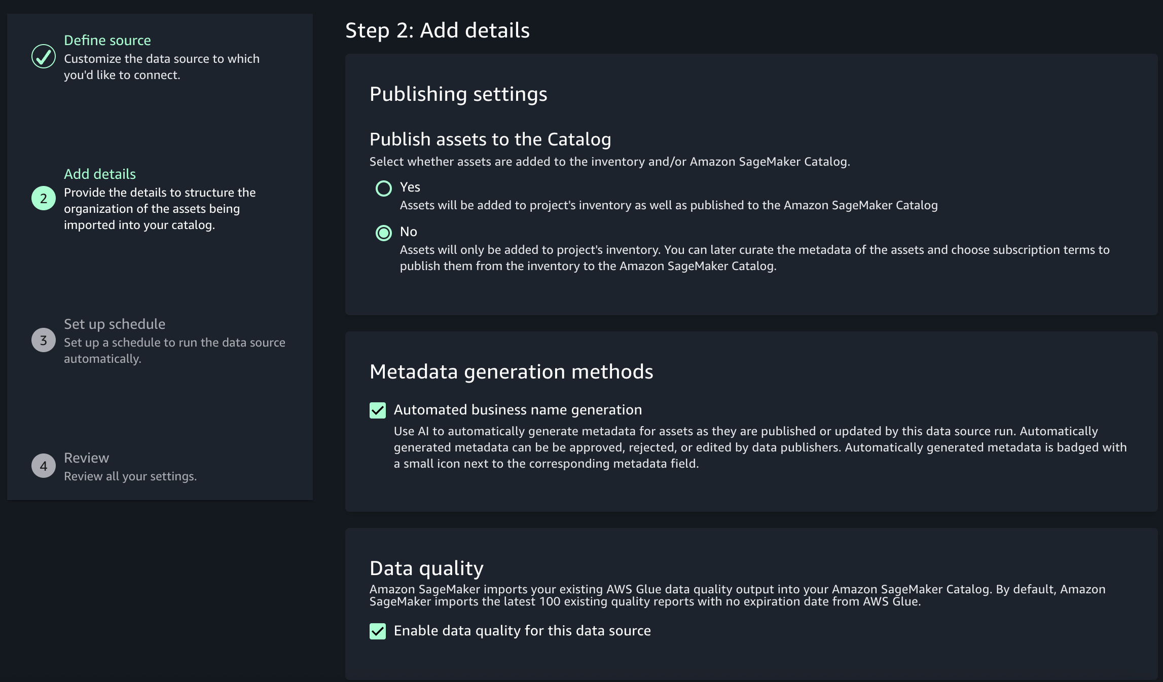
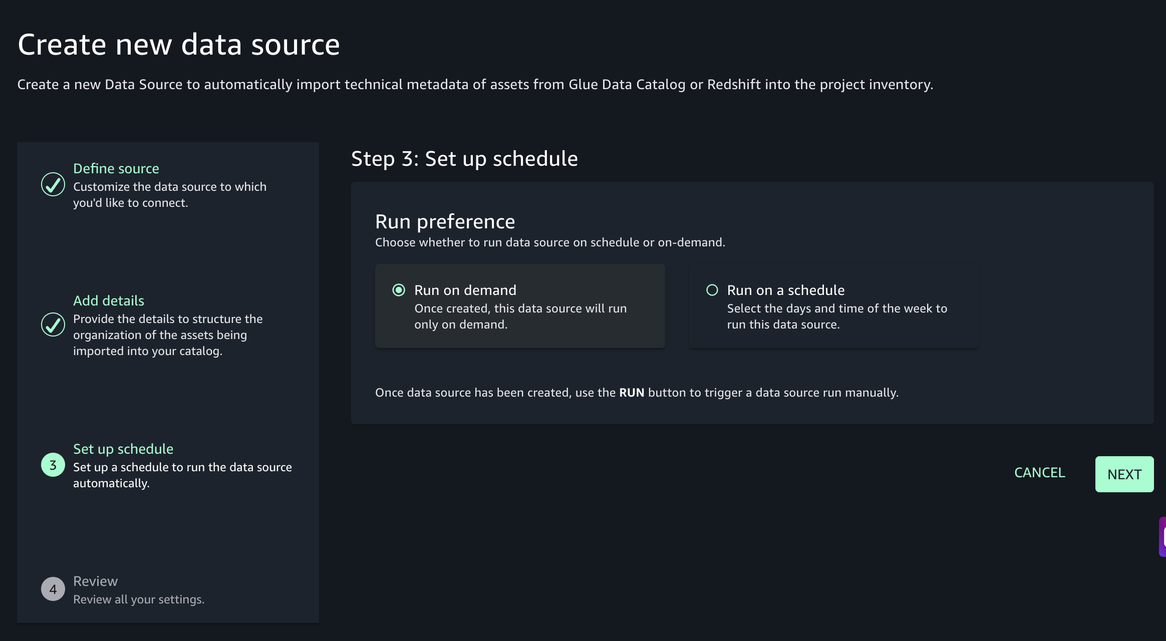
  7. Keep the default options and choose Next until you reach the summary screen.

    SageMaker Unified Studio data source configuration summary screen
    Data source review screen before creation
  8. Review your settings and choose Create.

To extract metadata and publish assets:

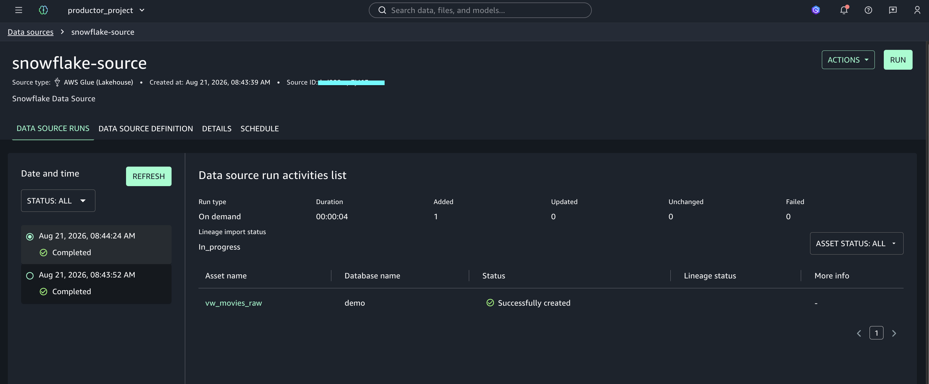
  1. Choose Run to start extracting metadata from AWS Glue Data Catalog.

    Data source detail page with the Run option to extract metadata from the AWS Glue Data Catalog
  2. Wait for the run to complete.
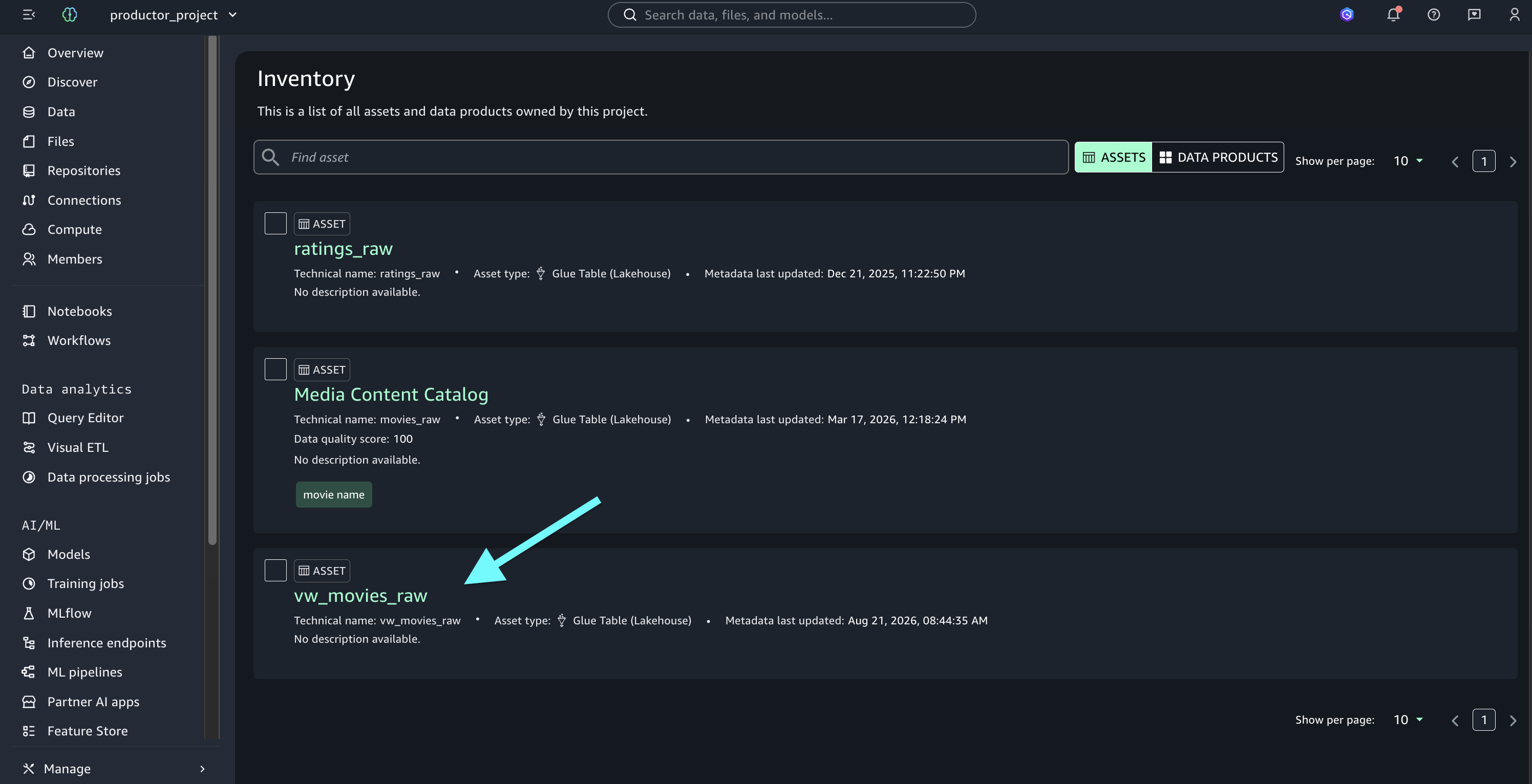
  3. Go to Assets to view the Asset Inventory.

    Asset inventory in SageMaker Catalog after the data source run completes

The following screenshot shows the asset inventory after the data source run completes.

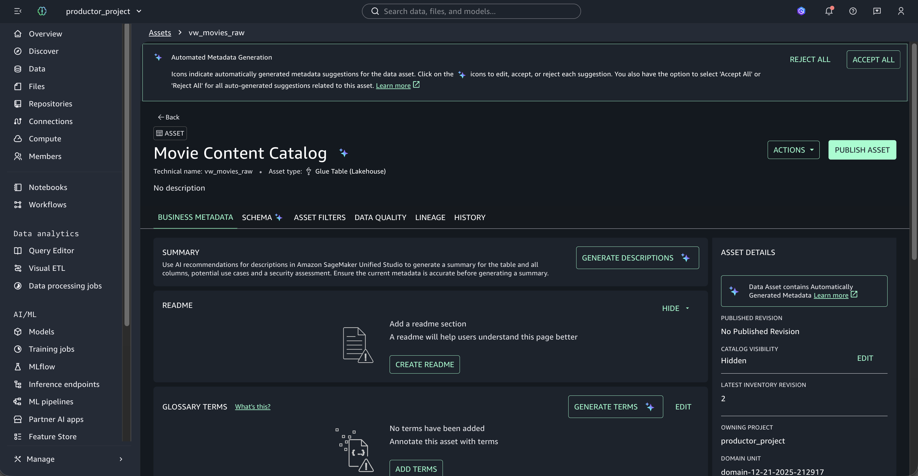
  1. Choose an asset to view its details.

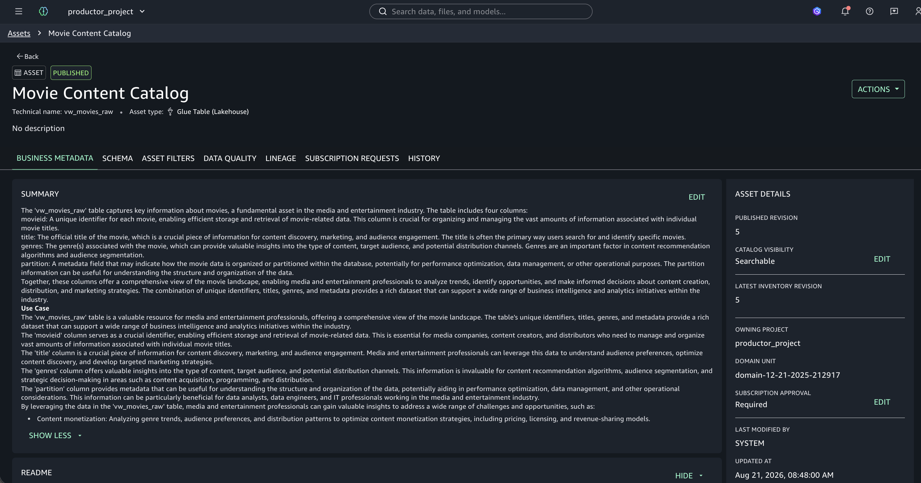
    Asset detail page in SageMaker Catalog showing the Snowflake table metadata

At this point, you can enrich the business context by choosing Generate Descriptions. Amazon SageMaker Catalog analyzes the asset’s technical structure and generate:

  • Business descriptions in natural language for the asset.
  • Contextual definitions for each field/column.
  • Suggested glossary terms that could be applied.
  1. After your asset has been enriched with the necessary business metadata, you can publish it to the Amazon SageMaker Catalog by choosing Publish Asset.

Publish Asset option on the enriched Snowflake asset in SageMaker Catalog

The Snowflake enriched asset is now available to data consumers across your organization. Other users can discover it, subscribe to it, and consume it without data replication.

Implementing data quality rules with AWS Glue Data Quality

This section explains how to apply data quality validations to Snowflake data using AWS Glue Data Quality and visualize results in Amazon SageMaker Catalog.

Setting up the custom transform

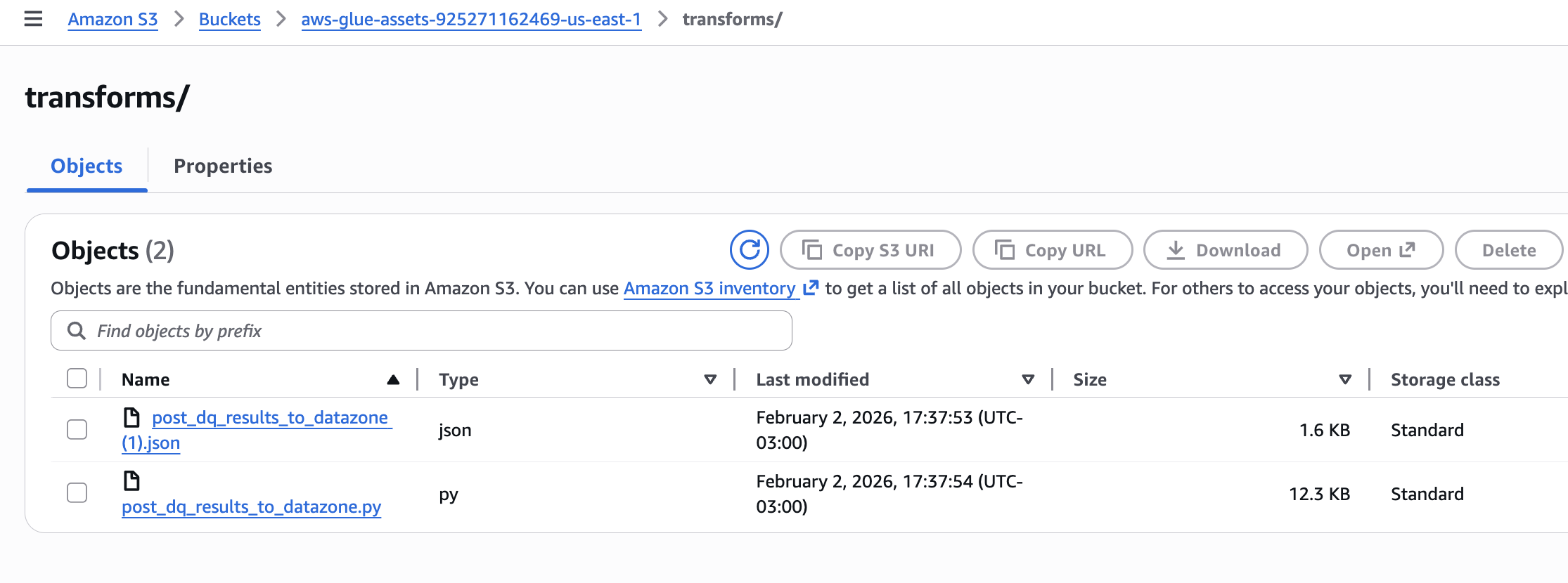
Upload two files to an Amazon S3 bucket in the same AWS account where you run AWS Glue:

Copy both files to your AWS Glue assets S3 bucket in the transforms folder (s3://aws-glue-assets-<account-id>-<region>/transforms). AWS Glue Studio reads all JSON files from this folder to register custom visual transforms.

Custom transform files uploaded to the transforms folder in the AWS Glue assets S3 bucket

In the following sections, we walk you through the steps of building an ETL pipeline for data quality validation using AWS Glue Studio.

Creating the AWS Glue Visual ETL job

AWS Glue for Spark provides built-in support for reading from Snowflake data sources.

To create a new visual ETL job:

  1. Open the AWS Glue console at https://console.aws.amazon.com/glue/. Choose ETL jobs, then Visual ETL.

    AWS Glue console showing ETL jobs and the Visual ETL option

Establishing the Snowflake connection

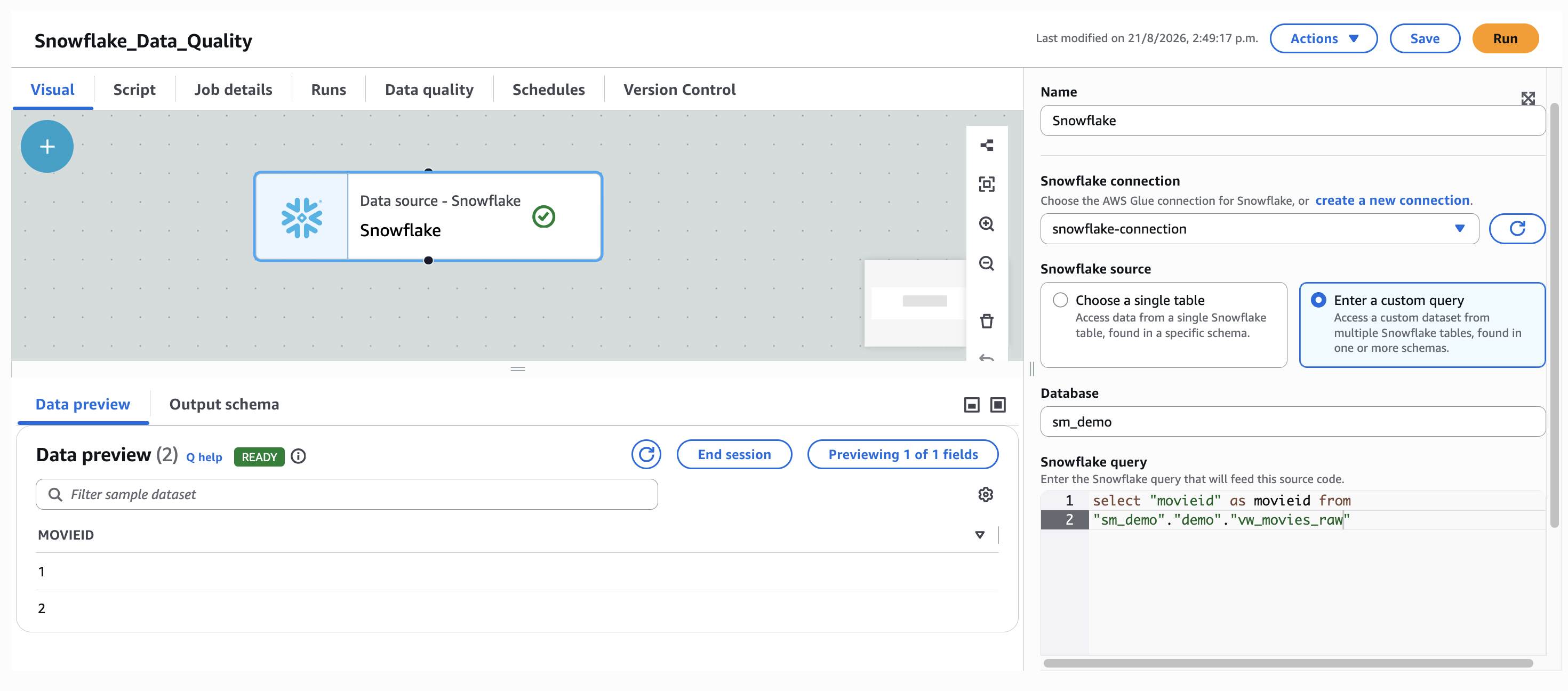
To add a Snowflake source:

  1. In the job pane, choose Snowflake as your source. For Snowflake connection, select the connection that you created earlier. Specify the relevant schema and table for data quality checks.

    Snowflake source node configured in the AWS Glue visual ETL job

The visual editor displays the Data source properties panel where you select your connection, database, and enter a custom query targeting your Snowflake table.

Applying data quality rules

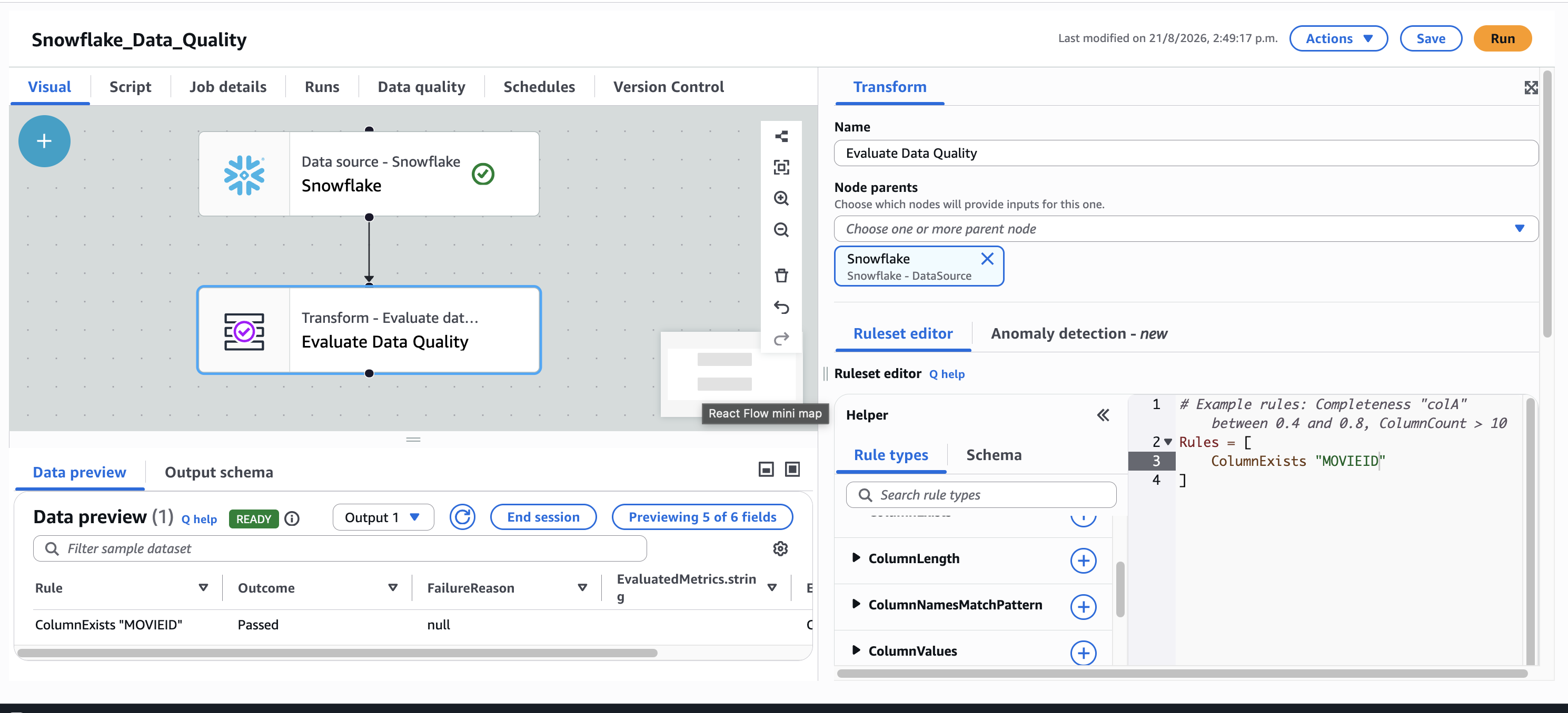
After establishing the Snowflake connection, configure the data quality evaluation step using the Data Quality Definition Language (DQDL).

To add data quality validation:

  1. Choose Transform and choose Evaluate Data Quality.
  2. Define domain-specific data quality rules using DQDL. For more information, see the AWS DQDL documentation.

    Evaluate Data Quality transform with DQDL rules in AWS Glue Studio
  3. Choose to output the data quality results. Optionally, store outcomes in Amazon S3 or publish to Amazon CloudWatch with alert notifications.

The preview of the data quality results from the ruleOutcomes node shows the outcomes of each rule.

Preview of the data quality rule outcomes from the ruleOutcomes node

Post the data quality results to Amazon SageMaker Catalog

To configure the custom transform:

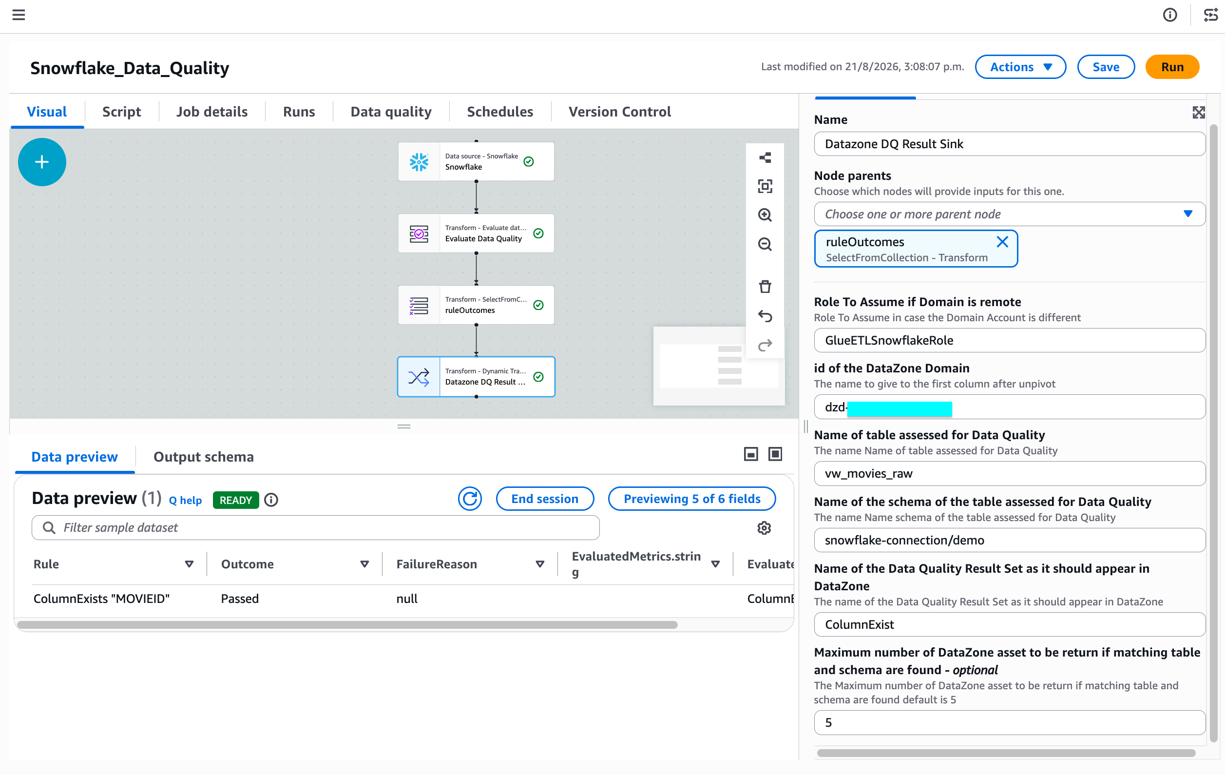
  1. Add the Datazone DQ Result Sink transform to your job.
  2. Connect the ruleOutcomes node output to this transform.
  3. Complete the parameters:
    • Role to assume (Optional): Only needed for associated accounts.
    • Domain ID: Your Amazon SageMaker Unified Studio domain ID (found in the Amazon SageMaker Unified Studio portal).
    • Table name and Schema name: Same values used when creating the Snowflake source transform.
    • Data quality ruleset name: The name you want to give to the ruleset in Amazon SageMaker Catalog.
    • Max results: Maximum number of assets to return in case of multiple matches.

The following image shows the complete job graph with the Datazone DQ Result Sink transform configured.

AWS Glue visual ETL job graph with Snowflake source, Evaluate Data Quality, ruleOutcomes, and Datazone DQ Result Sink nodes

The visual editor displays four nodes connected sequentially: the Snowflake data source, the Evaluate Data Quality transform, the ruleOutcomes SelectFromCollection transform, and the Datazone DQ Result Sink transform.

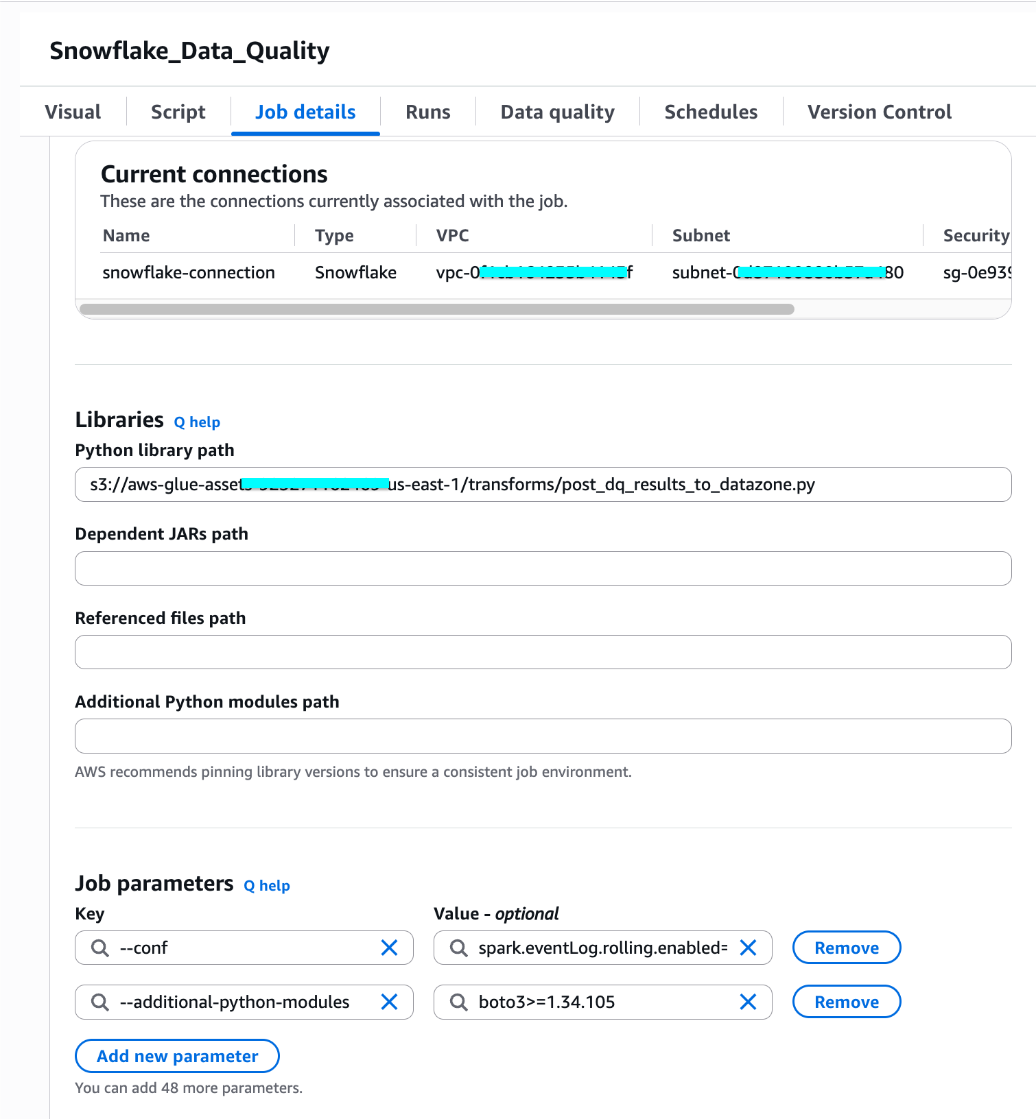
To configure job parameters:

  1. Choose Job details.
  2. In Job parameters, add the following key-value pair:
    • --additional-python-modules
    • boto3>=1.34.105
  3. Save and run the job.

AWS Glue job parameters with the additional-python-modules key set to boto3

Visualizing data quality results in the SageMaker Catalog

After the AWS Glue ETL job completes, you can view the data quality information directly in Amazon SageMaker Catalog. This is the key outcome of running data quality on a federated source: the asset gains quality scores and metadata without ever leaving Snowflake. This makes it trustworthy and ready for other teams across your organization to use. Data consumers can now discover this asset in Amazon SageMaker Catalog and evaluate its quality before subscribing, without needing direct access to Snowflake or running their own validation.

To view data quality results:

  1. Open the Amazon SageMaker Unified Studio console.
  2. Navigate to your project.
  3. Go to Assets.
  4. Choose the Snowflake data asset.
  5. View the data quality information displayed on the asset page.

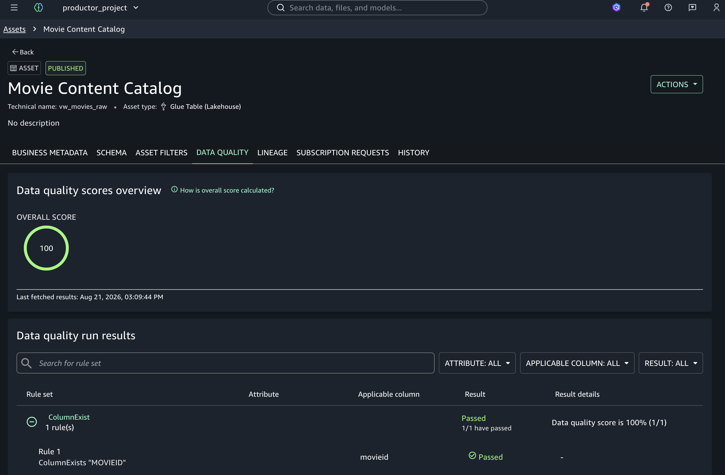
The following image shows the asset page in Amazon SageMaker Catalog with the data quality score populated.

SageMaker Catalog asset page showing a populated data quality score for the Snowflake asset

Data Quality tab in SageMaker Catalog showing an overall score of 100 with the movies rule set passed

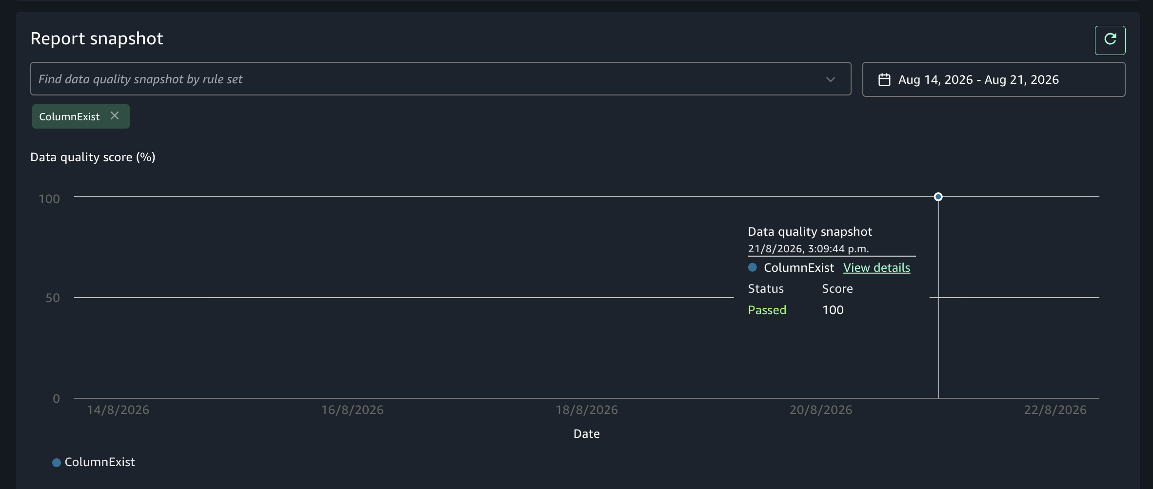
The Data Quality tab shows an overall score of 100 and lists the rule set movies with a Passed result (1/1). This confirms that the data quality checks from AWS Glue posted successfully to Amazon SageMaker Catalog.

Clean up

To avoid ongoing charges, remove the resources you created during this walkthrough:

  1. Delete the AWS Glue ETL job — Open the AWS Glue console, choose ETL jobs, select your job, and then choose Delete.
  2. Remove the AWS Glue connection — In the AWS Glue console, go to Connections, select the Snowflake connection, and then choose Delete.
  3. Delete the data source in SageMaker Catalog — In your Amazon SageMaker Unified Studio project, go to Data Sources, select the data source you created, and then choose Delete.
  4. Remove S3 assets — Delete the custom transform files from your s3://aws-glue-assets-<account-id>-<region>/transforms/ bucket.
  5. Remove IAM policies — Detach and delete the IAM policies you attached to the AWS Glue job execution role. Remove the role as a domain user and project member.

Conclusion

In this post, we showed you how to connect Snowflake to Amazon SageMaker Unified Studio for centralized data cataloging and quality validation. This approach maintains consistent governance without replicating data. Key benefits include:

  • Query without data movement: Access Snowflake data directly from Amazon SageMaker Unified Studio through federated queries, using the interoperable data architecture of AWS and eliminating time-consuming data replication.
  • Centralized governance: Maintain a single source of truth for data discovery, quality metrics, and governance policies across your distributed data estate.
  • Automated quality validation: Apply consistent data quality rules using AWS Glue Data Quality and visualize results directly in Amazon SageMaker Catalog.
  • Unified collaboration: Support data discovery and sharing across your organization through the publishing capabilities of Amazon SageMaker Catalog.

To get started, open the Amazon SageMaker Unified Studio console. To learn more about related topics, see Cross-account lakehouse governance with Amazon S3 Tables and SageMaker Catalog and Get started with AWS Glue Data Quality dynamic rules for ETL pipelines.


About the authors

Marco Duarte López

Marco Duarte López

Marco is a Data Specialist Solutions Architect at AWS, based in Santiago, Chile. He works with organizations across the region to design modern data architectures and governance frameworks that enable trusted, scalable data consumption. He is a member of the AWS Technical Field Community (TFC) for Analytics, where he specializes in Data & AI Governance, and has led data transformation programs for some of the largest enterprises in the region.

Diego Ortiz

Diego Ortiz

Diego is a Senior Data Strategy Solutions Architect for Latin America based in San Juan, Puerto Rico, with 14+ years of experience in technology roles. He supports organizations across countries and industries to develop data and AI strategies aligned with their business objectives, combining strategic vision with deep technical expertise in data and AI technologies. He is a core member of the Data Governance global community at AWS and leads the analytics technical community in the Spanish-speaking countries of Latin America.

Connect Amazon SageMaker Unified Studio to Microsoft Power BI – Part 1: IAM Identity Center (IDC)-based domains

Post Syndicated from Ramesh H Singh original https://aws.amazon.com/blogs/big-data/connect-amazon-sagemaker-unified-studio-to-microsoft-power-bi-part-1-iam-identity-center-idc-based-domains/

Connecting Power BI to your Amazon SageMaker Unified Studio data catalogs typically required third-party bridges. These bridges added complexity and licensing costs. In this post, you create a direct connection using new authentication modes in the Amazon Athena ODBC driver, removing those dependencies entirely. If your organization uses Power BI as its business intelligence (BI) tool, your analysts can configure access to governed data in Amazon SageMaker Unified Studio without changing their tools or workflows. As an AWS alternative, Amazon Quick Sight provides serverless BI integration with Amazon SageMaker Unified Studio at pay-per-session pricing.

A previous post showed the connection method using a third-party ODBC-JDBC bridge. The Amazon Athena ODBC driver (version 2.2.0 and later) now supports Amazon SageMaker Unified Studio authentication directly, eliminating the need for customers to configure third-party bridge components previously required for this connection. This bridge also created additional components and required ongoing maintenance. The native connection simplifies the architecture by reducing these requirements.

UC Irvine, a top-ten U.S. public research university, consolidates student data from systems across multiple departments into a single governed repository that supports reporting, research, and analytics for decision-making at the strategic, tactical, and operational levels. Many of their analysts rely on Power BI to explore and visualize this governed data.

“Our users rely on Power BI for data visualization and reporting, but connecting to governed data in AWS previously required workarounds. The ODBC connection feature gives a direct path from Power BI into our SageMaker Unified Studio projects—no bridge software, no extra licensing, just a connection string and we’re ready to go.”

— Bernadette Theologidy, Manager, Student Analytics, UC Irvine

The Athena ODBC driver introduces two new authentication modes for SageMaker Unified Studio:

  1. SageMakerBrowserIdc (for IDC-based domains): The driver opens a browser window and authenticates through AWS IAM Identity Center (and your external identity provider, if configured). No local AWS credentials are needed.
  2. SageMakerIam (for AWS Identity and Access Management (IAM)-based and IDC-based domains): The driver uses AWS credentials from the default credential provider chain. For this walkthrough, we use AWS IAM Identity Center to provide those credentials.

You connect Microsoft Power BI to Amazon SageMaker Unified Studio through Athena. The Athena ODBC driver supports using two connection methods that use these authentication modes:

Method 1: DSN-based (Athena Power BI connector): You configure an ODBC Data Source Name (DSN) and use the Athena connector in Power BI. This method supports DirectQuery and Import mode with both SageMakerBrowserIdc and SageMakerIam authentication.

Method 2: DSN-less (Power BI ODBC connector): You use the Power BI ODBC connector with a connection string, requiring no DSN configuration. This method supports Import mode only with SageMakerIam authentication. DirectQuery isn’t available because the Power BI ODBC connector doesn’t support it. The connection string in Power BI Desktop must match exactly the one on Power BI Service. Because the gateway runs as a Windows service without interactive browser access, both ends must use SageMakerIam.

Feature Method 1: DSN-based Method 2: DSN-less
Power BI Connector Amazon Athena connector ODBC connector
Data connectivity mode DirectQuery and Import Import only
Requires DSN configuration Yes No
Data freshness Real-time (DirectQuery) or scheduled (Import) Scheduled refresh only
Authentication types SageMakerIam and SageMakerBrowserIdc SageMakerIam only
Domain types supported IAM-based and IDC-based IAM-based and IDC-based
Best for Dashboards requiring live data Scenarios where DSN management is not possible or scheduled refresh is acceptable

This is Part 1 of a two-part series. This post covers IDC-based domains using both connection methods. Part 2 covers IAM-based domains.

Solution overview

In this walkthrough, you take the role of a data analyst at an energy company. You need to understand the current state and future direction of the U.S. power generation fleet using the Public Utility Data Liberation Project, available on the Registry of Open Data on AWS. Our goal is to analyze generation capacity and identify where new investment is flowing. We connect Power BI to Athena through Amazon SageMaker Unified Studio and query the EIA-860 generators dataset directly from our data catalog. The result is a single visualization that reveals the energy transition.

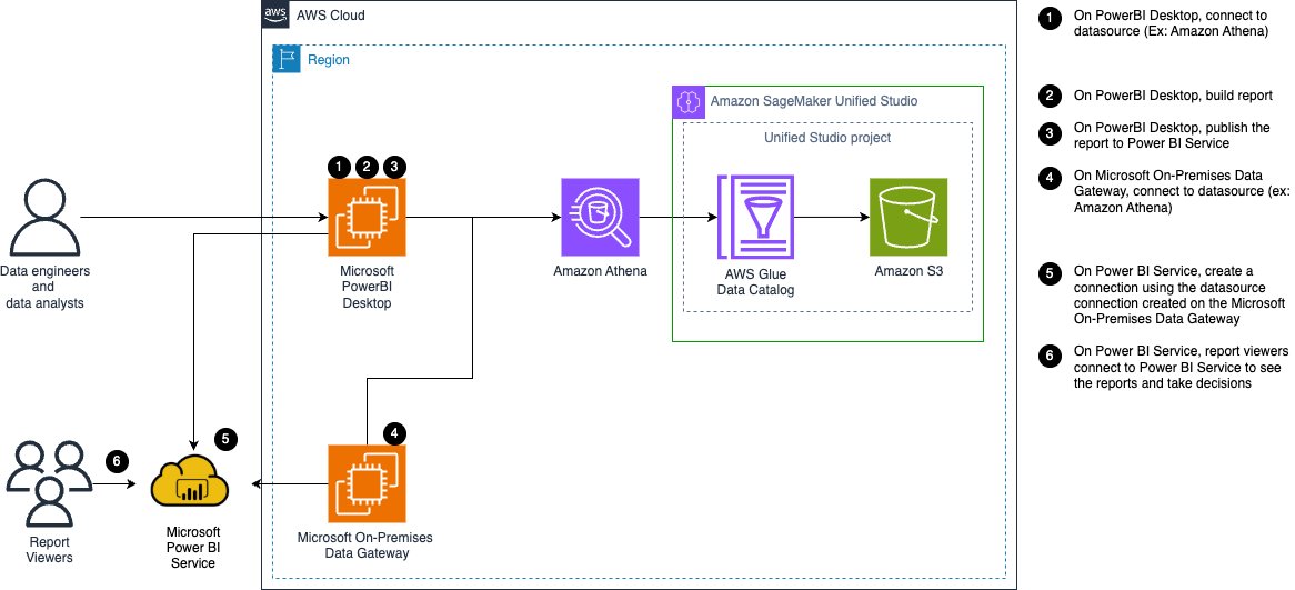
The following diagram illustrates the solution architecture for connecting Power BI to Amazon SageMaker Unified Studio through Amazon Athena.

Architecture diagram showing Power BI connecting to Amazon Athena through Amazon SageMaker Unified Studio, with a Microsoft on-premises data gateway on Amazon EC2

Figure 1: Architecture diagram

The following architecture demonstrates a six-step workflow.

  1. Data engineers and analysts connect Power BI Desktop to Athena as a data source.
  2. They build their reports locally.
  3. They then publish them to the Power BI Service.
  4. Microsoft On-Premises Data Gateway on an Amazon Elastic Compute Cloud (Amazon EC2) instance connects to Athena using the instance’s attached IAM role.
  5. The Power BI Service then uses this gateway connection.
  6. Report viewers access the published reports through Power BI Service to make data-driven decisions.

On the AWS side, Athena queries the data catalog managed by AWS Glue Data Catalog. The catalog references data stored in Amazon Simple Storage Service (Amazon S3). An Amazon SageMaker Unified Studio project governs all access.

In an IDC-based domain (covered in this post), Power BI Desktop uses SageMakerBrowserIdc for Method 1 and SageMakerIam for Method 2. Power BI Desktop can run on-premises or on an EC2 instance. The gateway always uses SageMakerIam (it runs as a Windows service without browser access) and authenticates using instance profile credentials, which rotate automatically. The gateway can only query data within projects where its IAM role has been added as a member. For IAM-based domains, see Part 2.

Prerequisites

Before connecting Power BI to Amazon SageMaker Unified Studio, verify that your environment meets these requirements:

  • Athena ODBC driver – The latest Amazon Athena ODBC driver (version 2.2.0 or more recent) for Windows 64-bit.
  • Microsoft Power BI Desktop – The latest version installed on your Windows machine.
  • Microsoft Power BI Pro License – Required for publishing reports and configuring the on-premises data gateway.
  • Microsoft Power BI on-premises data gateway – The latest version installed on the EC2 instance.
  • Amazon SageMaker Unified Studio – An Amazon SageMaker Unified Studio IDC-based domain.

You need an Amazon SageMaker Unified Studio project with data assets. For detailed instructions, refer to the Amazon SageMaker Unified Studio User Guide.

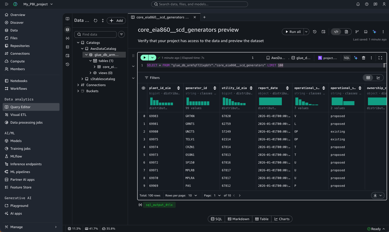
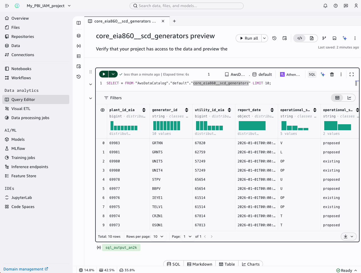
The following screenshot shows the Amazon SageMaker Unified Studio project Query Editor interface, which runs a preview query against the EIA-860 generators dataset.

SageMaker Unified Studio Query Editor previewing the EIA-860 generators dataset

Figure 2: SageMaker Unified Studio project with the EIA-860 generators dataset available in the data catalog

Method 1: DSN-based connection (Athena Power BI connector)

This method uses the Amazon Athena Power BI connector with an ODBC Data Source Name (DSN), supporting DirectQuery and Import mode.

You configure Power BI Desktop to connect to your data assets in Amazon SageMaker Unified Studio using the SageMakerBrowserIdc authentication mode. The driver opens a browser window and authenticates through IAM Identity Center (and your external identity provider, if configured).

Add your SSO user as a member of your SageMaker Unified Studio project

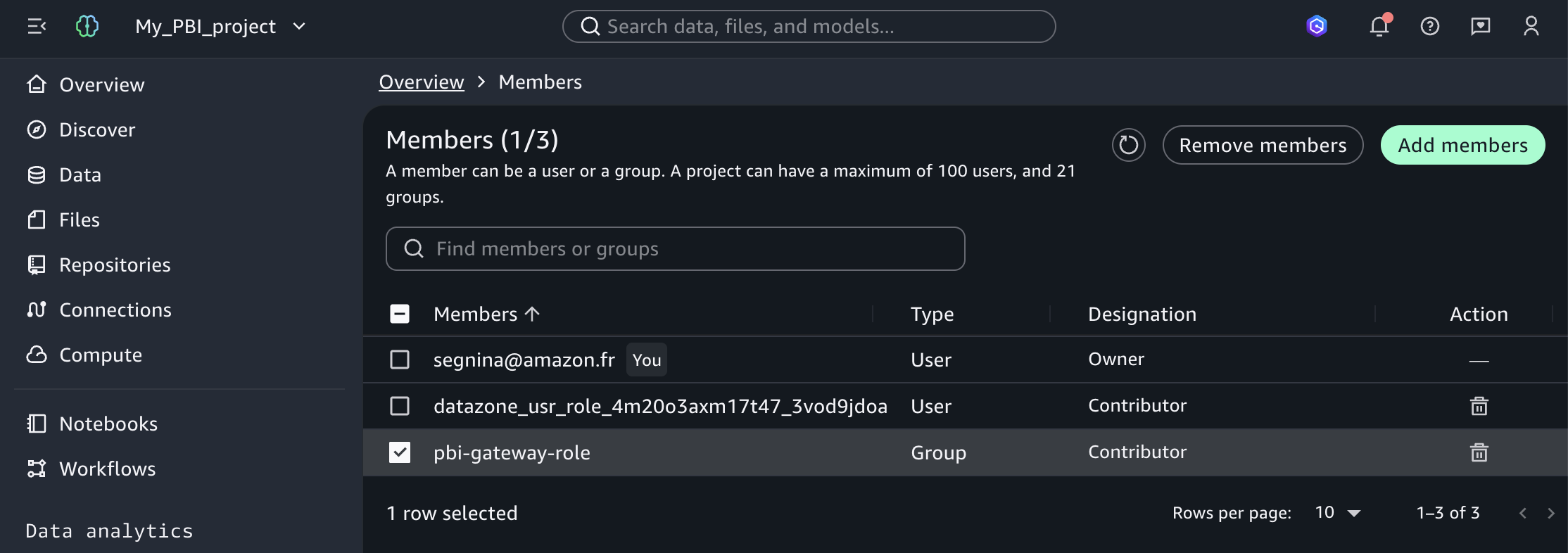
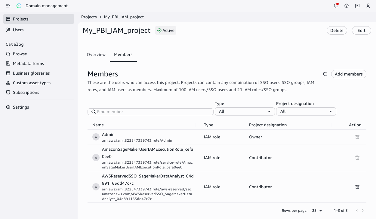
Your single sign-on (SSO) user needs project-level access to query data with Athena. Verify your user is listed as a project member or add it by following Add project members in the Amazon SageMaker Unified Studio User Guide.

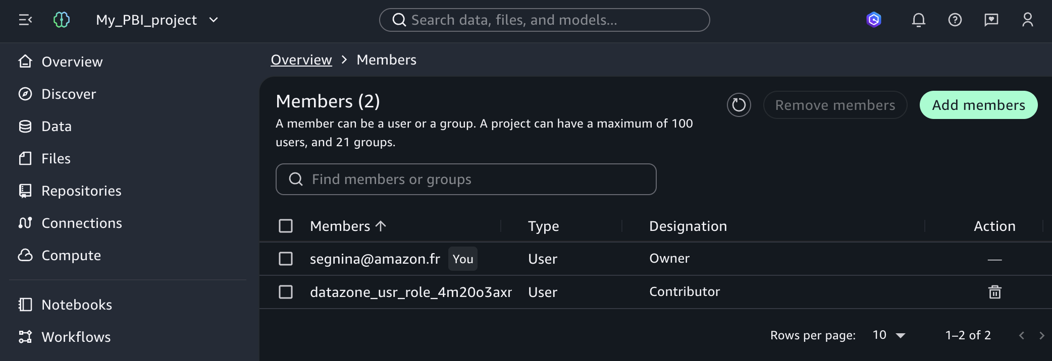
The following screenshot shows the SageMaker Unified Studio project user management page, where project owners can add or remove project users and roles.

SageMaker Unified Studio project members page listing users and roles

Figure 3: Members of a SageMaker Unified Studio project

Gather configuration values to configure your Amazon Athena ODBC DSN

Gather the following values from your Amazon SageMaker Unified Studio project:

  1. Open your Amazon SageMaker Unified Studio project.
  2. In the top right, select the three dots.
  3. Choose Project details.
  4. Select JDBC and ODBC details.
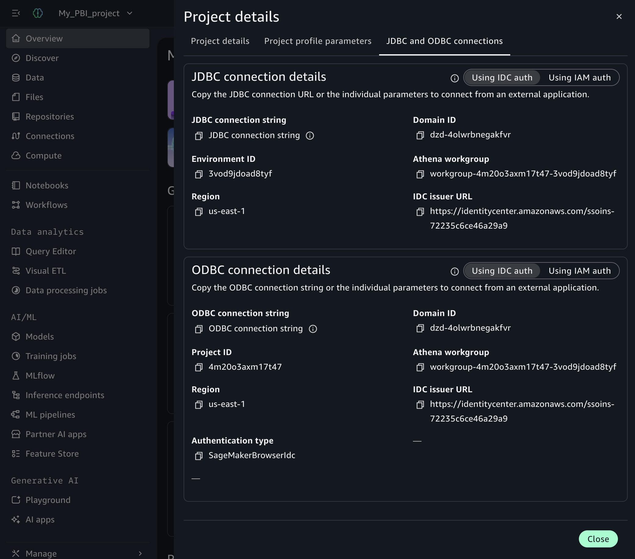
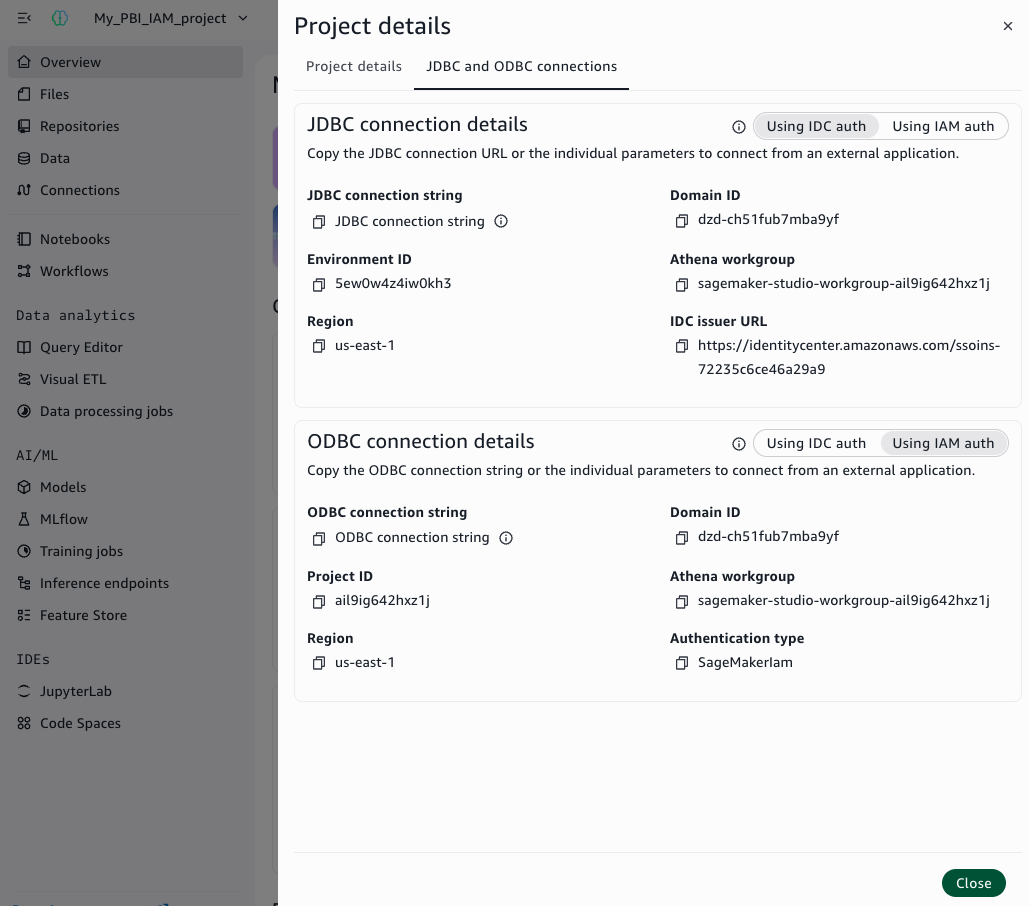
  5. Under ODBC connection details copy the following information: IDC issuer URL, domain ID, project ID, Athena workgroup name and AWS Region.

The following screenshot shows the Amazon SageMaker Unified Studio project overview page, where you can copy these details.

SageMaker Unified Studio project overview showing ODBC connection details

Figure 4: ODBC connection details

Configure the ODBC DSN

Create a System DSN using the Amazon Athena ODBC driver. For the general DSN creation steps, see Configuring a data source name on Windows in the Amazon Athena User Guide.

Enter the following values:

Field Value
Data Source Name Name your datasource (for example, pbi-idcdomain)
Region The AWS Region where your Amazon SageMaker domain is provisioned (for example, us-east-1)
Catalog AwsDataCatalog
Database default
Workgroup Your Athena workgroup name (for example, workgroup-abcdefghij-klmexample)

In the Authentication Options, configure the following values:

Field Value
Authentication Type SageMakerBrowserIdc
SSO Start URL IAM Identity Center entry point (for example, https://identitycenter.amazonaws.com/ssoins-0example)
SSO Region Region of IAM Identity Center (for example, us-east-1)
SageMaker Domain ID dzd-123456example
SageMaker Project ID abcd12example
SageMaker Domain Region Region of your Amazon SageMaker Unified Studio project (for example, us-east-1)

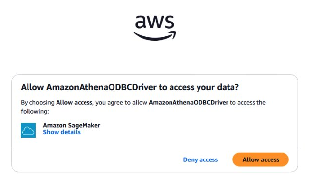
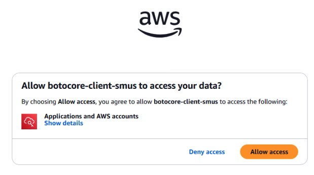
Choose OK, then Test to verify the connection. Choose Allow Access when prompted by the browser.

The following screenshot shows the consent prompt.

Browser consent prompt requesting access approval during authentication

Figure 5: Browser consent prompt

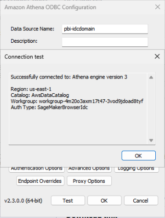
The following screenshot shows the successful connection test.

ODBC DSN configuration showing a successful connection test with SageMakerBrowserIdc

Figure 6: Successful connection test in the ODBC DSN configuration with SageMakerBrowserIdc authentication

Connect Power BI Desktop to your data

With the DSN configured, you can connect Power BI Desktop to your data catalog and load the generators dataset.

  1. Open Power BI Desktop.
  2. Open the Get Data menu and select More.
  3. Search for and select Amazon Athena and choose Connect.
  4. For Data Source Name (DSN), enter pbi-idcdomain.
  5. Select DirectQuery.
  6. Choose OK.
  7. Choose Use Data Source Configuration and then Connect.
  8. In the AwsDataCatalog folder, navigate to your database.
  9. Select the core_eia860__scd_generators table.
  10. Choose Load.

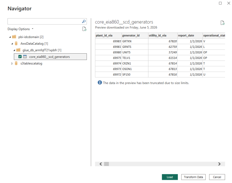
The following screenshot shows Power BI Desktop successfully connected to the AWS data catalog.

Power BI Desktop connected to the data catalog with the generators table loaded

Figure 7: Power BI Desktop connected to the data catalog with the generators table loaded using SageMakerBrowserIdc authentication

Create your dashboard and publish it

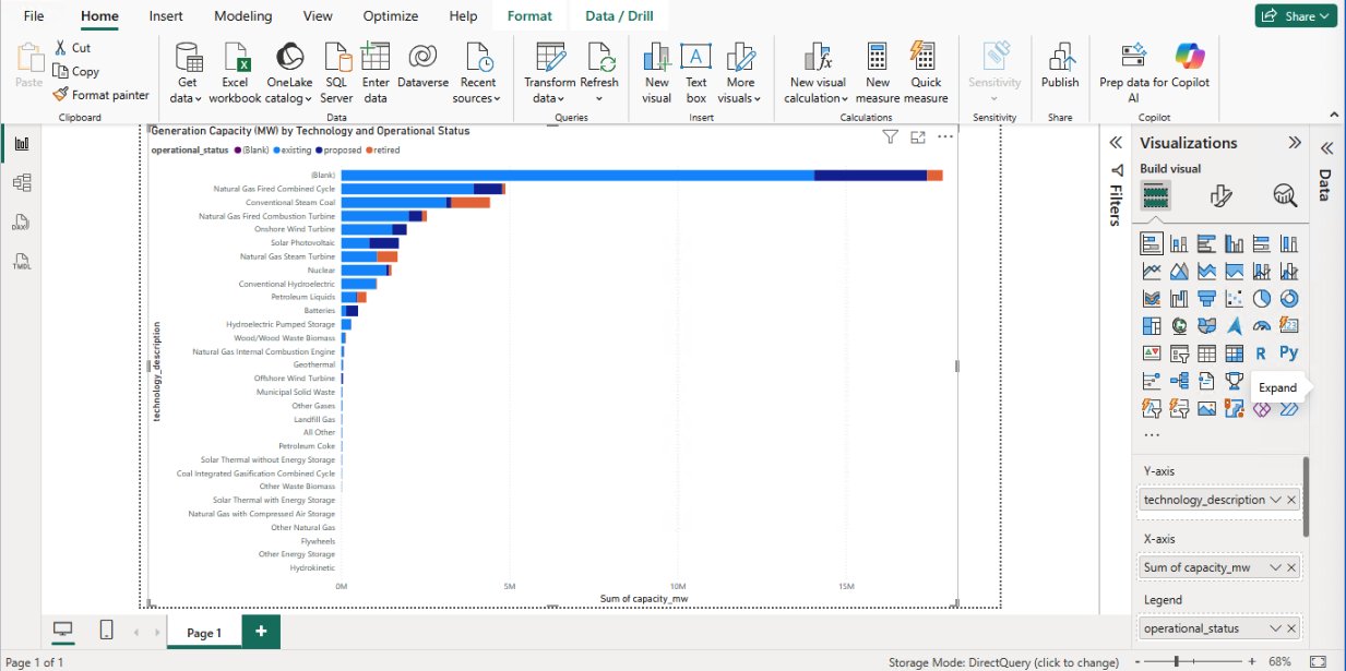
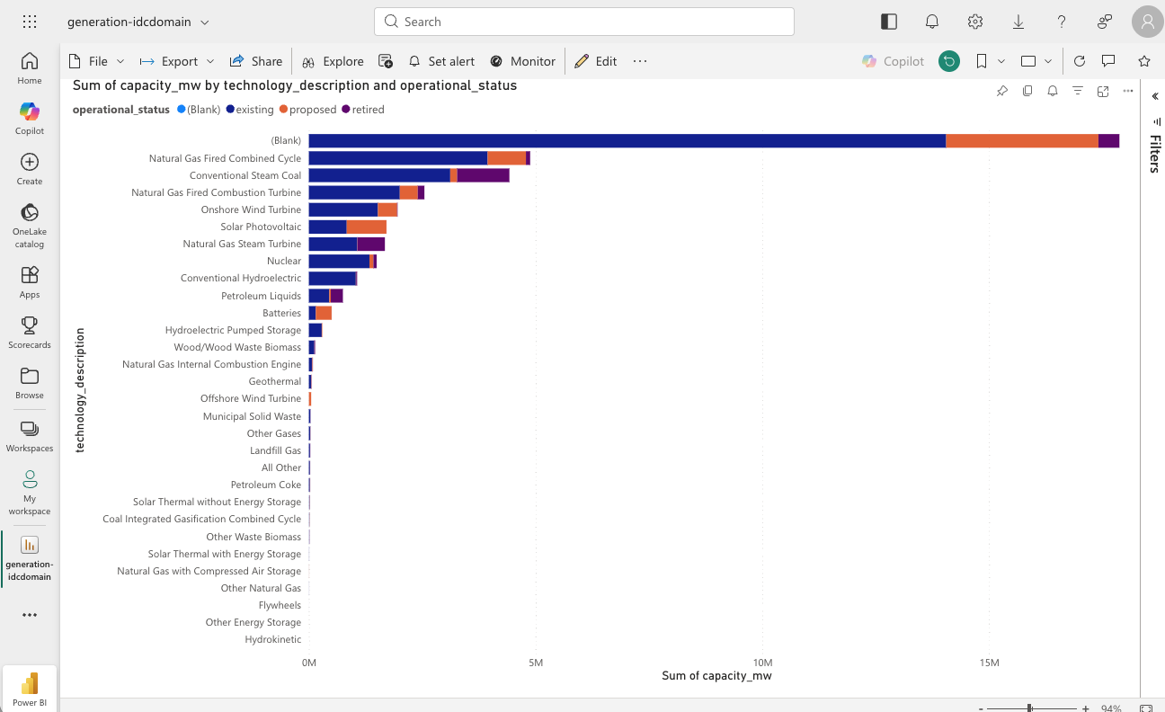
You can create a dashboard to visualize U.S. power generation data. To create a visualization, complete the following steps:

  1. In the Visualizations pane, choose the Stacked bar chart.
  2. Assign the Y-Axis: Drag technology_description to the Y-Axis.
  3. Assign the X-Axis (Values): Drag capacity_mw to the X-Axis (automatically summed).
  4. Assign the Legend (Stack): Drag operational_status to the Legend field.
  5. Choose Publish.
  6. Give your report a name (for example, generation-idcdomain) and choose Save.
  7. Sign in and choose a destination workspace.
Power BI Desktop stacked bar chart of generation capacity by technology and operational status

Figure 8: Power BI Desktop report using the EIA-860 generators dataset

After publishing, the report structure is available on Power BI Service.

Method 2: DSN-less connection (Power BI ODBC connector)

In this method, you use the Power BI ODBC connector with a connection string (no DSN required). This method supports Import mode only and SageMakerIam authentication. Because the gateway cannot perform browser authentication, both Desktop and gateway must use SageMakerIam. If your workflow requires SageMakerBrowserIdc, use Method 1.

If your machine already has AWS credentials through another method in the default credential provider chain, skip the following setup.

Administrator setup

Create a custom permission set named SageMakerDataAnalyst in IAM Identity Center with the following inline policy. For detailed steps, see Create a permission set in the AWS IAM Identity Center User Guide.

{
    "Version": "2012-10-17",
    "Statement": [
        {
            "Sid": "SageMakerAccess",
            "Effect": "Allow",
            "Action": [
                "datazone:GetConnection",
                "datazone:ListConnections",
                "datazone:GetDomain",
                "datazone:GetProject"
            ],
            "Resource": "*"
        },
        {
            "Sid": "STSForDriver",
            "Effect": "Allow",
            "Action": [
                "sts:GetCallerIdentity"
            ],
            "Resource": "*"
        }
    ]
}

Assign your user to this permission set for the AWS account containing your SageMaker Unified Studio domain. Then configure your AWS Command Line Interface (AWS CLI) SSO profile by running aws configure sso. For the full CLI configuration walkthrough with detailed steps, see Part 2. After your profile is configured, run aws sso login to authenticate.

Add the IAM identity as a member of SageMaker Unified Studio project

The IAM identity providing credentials needs both domain-level and project-level access to query data through Athena.

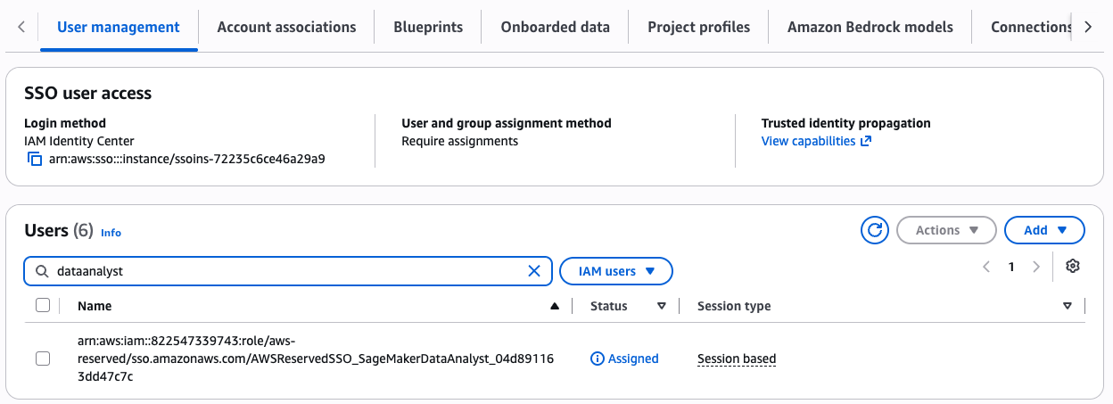
  1. Add AWSReservedSSO_SageMakerDataAnalyst_1234example as a domain IAM user: see Managing users in the Amazon SageMaker Unified Studio Admin Guide. Choose Current account.
SageMaker Unified Studio domain users list including the IAM identity

Figure 9: List of users of your SageMaker Unified Studio domain including the IAM identity

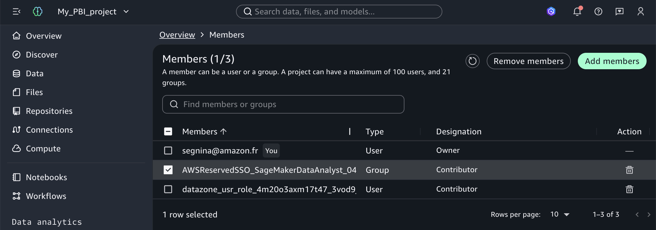
  1. Add AWSReservedSSO_SageMakerDataAnalyst_1234example as a project member: see Add project members in the Amazon SageMaker Unified Studio User Guide.
SageMaker Unified Studio project members list including the IAM identity

Figure 10: Members of a SageMaker Unified Studio project including the IAM identity

Gather configuration values

Gather the following connection values from your Amazon SageMaker Unified Studio project:

  1. Open your Amazon SageMaker Unified Studio Project.
  2. On the navigation pane, choose Overview.
  3. Select JDBC and ODBC details.
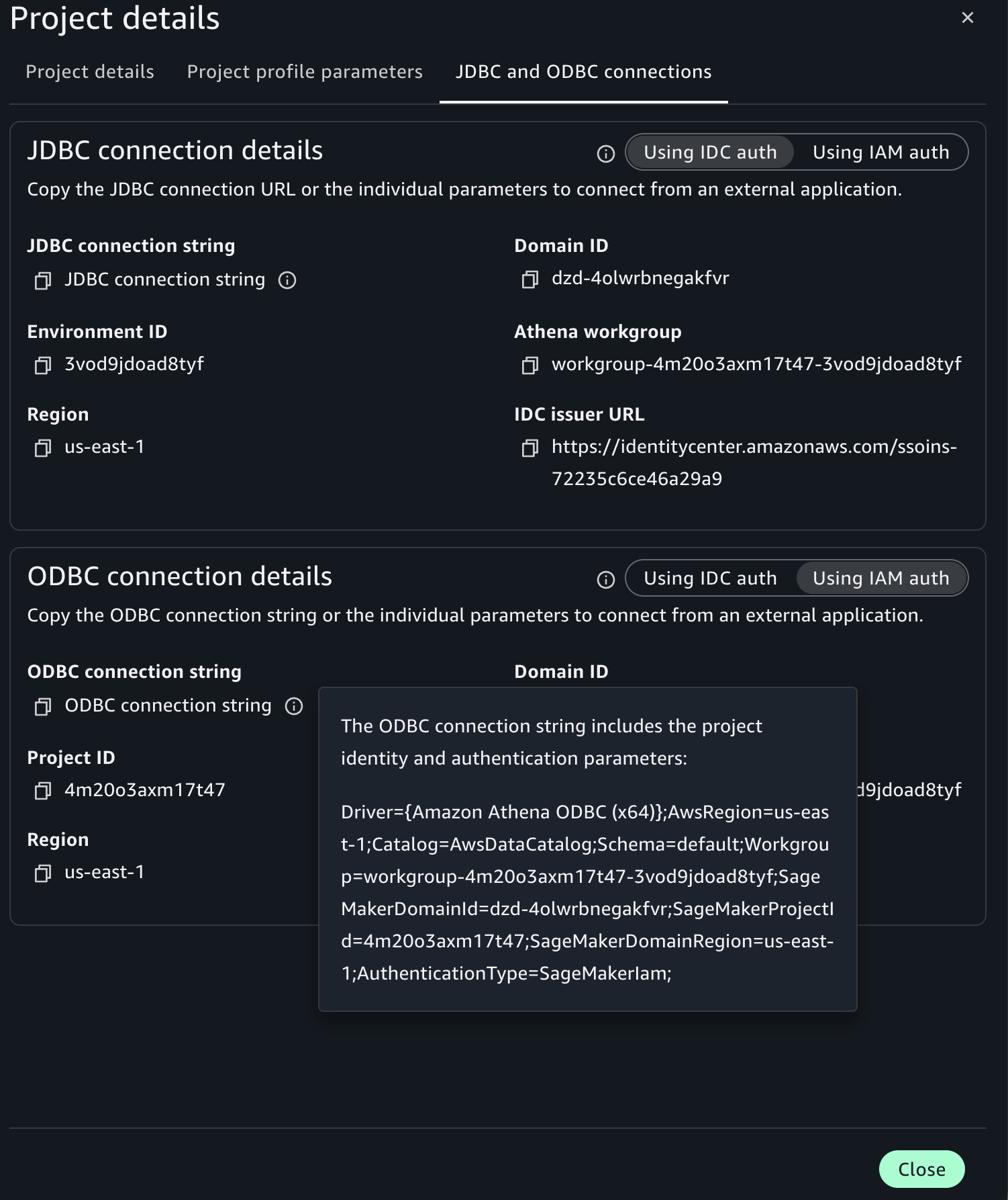
  4. Select the Using IAM auth toggle.
  5. Copy the ODBC connection string.
SageMaker Unified Studio project overview showing the ODBC connection string for IAM auth

Figure 11: ODBC connection string on the SageMaker Unified Studio project overview

Connect Power BI Desktop to your data and publish

With the configuration parameters of your project, you can connect Power BI Desktop to your data catalog and load the generators dataset.

  1. Open Power BI Desktop.
  2. Open the Get Data menu and select More.
  3. Search for and select ODBC and choose Connect.
  4. For Data Source Name (DSN), select (None).
  5. Expand Advanced Options.
  6. In the Connection string field, enter your connection string. For example, Driver={Amazon Athena ODBC (x64)};AwsRegion=us-east-1;Catalog=AwsDataCatalog;Schema=default;Workgroup=workgroup-abcdefghij-klmexample;SageMakerDomainId= dzd-123456example;SageMakerProjectId= abcd12example;SageMakerDomainRegion=us-east-1;AuthenticationType=SageMakerIam;
  7. Choose OK.
  8. Choose Default or Custom and then Connect.
  9. In the AwsDataCatalog folder, navigate to your database.
  10. Select the core_eia860__scd_generators table.
  11. Choose Load.

When publishing, name your report generation-idcdomain-dsnless.

Configure the on-premises data gateway and view your report on Power BI Service

After creating your reports in Power BI Desktop, configure the on-premises data gateway to view your report on Power BI Service.

You can configure the gateway using either a DSN or a DSN-less connection string, matching the method you used in Power BI Desktop.

Create and attach an IAM role to the Power BI Gateway EC2 instance

Create an IAM role for the EC2 instance that will host your Power BI gateway. Name the role pbi-gateway-role (or a name of your choice). The role must use EC2 as the trusted entity and include the following inline policy:

{
    "Version": "2012-10-17",
    "Statement": [
        {
            "Sid": "SageMakerAccess",
            "Effect": "Allow",
            "Action": [
                "datazone:GetConnection",
                "datazone:ListConnections",
                "datazone:GetDomain",
                "datazone:GetProject"
            ],
            "Resource": "*"
        },
        {
            "Sid": "STSForDriver",
            "Effect": "Allow",
            "Action": [
                "sts:GetCallerIdentity"
            ],
            "Resource": "*"
        }
    ]
}

Attach this role to your Power BI Gateway EC2 instance. For detailed steps on creating and attaching an IAM role to an EC2 instance, refer to IAM roles for Amazon EC2 in the Amazon EC2 User Guide.

Add the Power BI Gateway IAM role as a member of SageMaker Unified Studio project

The gateway IAM role needs project-level access to query data through Athena.

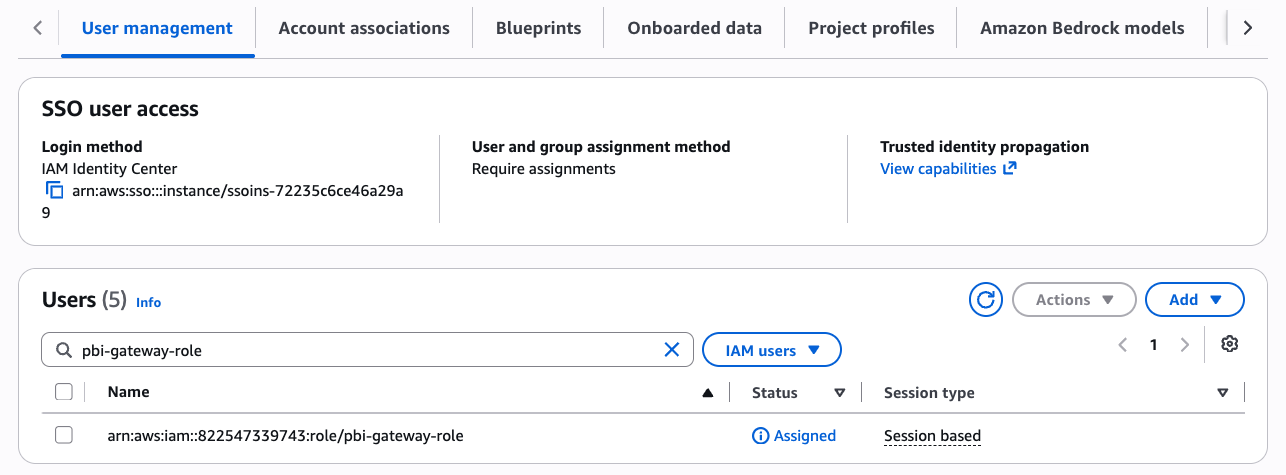
  1. Add the IAM pbi-gateway-role role as a domain IAM user: see Managing users in the Amazon SageMaker Unified Studio Admin Guide. Choose Current account (or Associated account if your gateway is deployed in a different account).

The following screenshot, from the Amazon SageMaker page of the AWS Management Console, shows the list of users of your Amazon SageMaker Unified Studio domain, including the IAM gateway role.

SageMaker Unified Studio domain users list including the Power BI gateway IAM role

Figure 12: List of users of your SageMaker Unified Studio domain including the IAM gateway role

Add the IAM pbi-gateway-role role as a project member: see Add project members in the Amazon SageMaker Unified Studio User Guide.

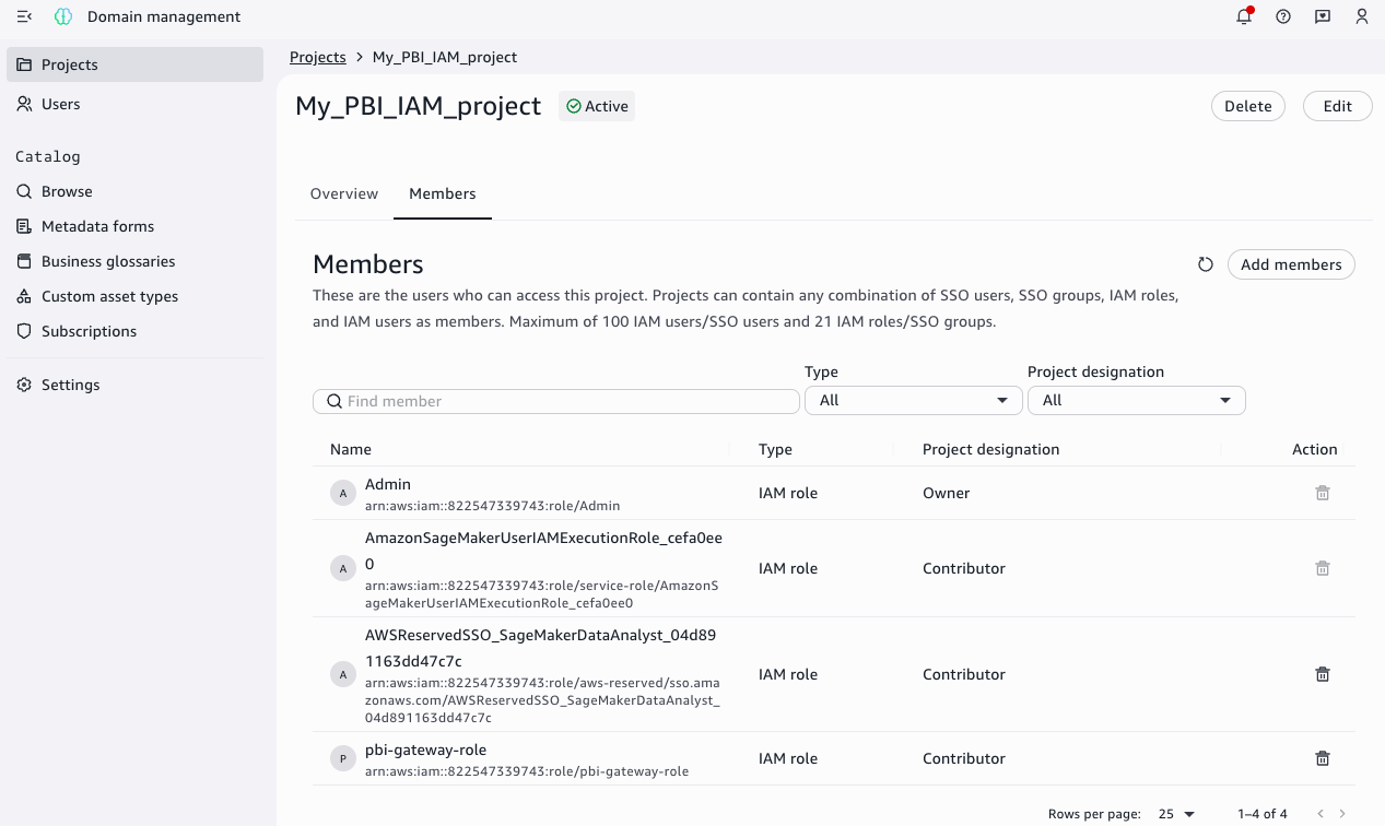
The following screenshot shows the Amazon SageMaker Unified Studio project user management page listing the project members.

SageMaker Unified Studio project members list including the Power BI gateway IAM role

Figure 13: Members of a SageMaker Unified Studio project including the IAM gateway role

Configure the data source on Power BI Gateway

How you configure the data source depends on the method you used in Power BI Desktop.

Method 1 (DSN-based)

Configure a System DSN on the gateway EC2 instance following the same ODBC DSN steps described in Method 1. When configuring, make sure that:

  • You use the System DSN tab (not User DSN) because the gateway runs as a Windows service under a separate account.
  • The authentication type is set to SageMakerIam regardless of what you used on Desktop.
  • The DSN name matches exactly the one configured on Power BI Desktop (for example, pbi-idcdomain)

Method 2 (DSN-less)

No configuration is needed on the gateway machine itself. You configure the data source directly in Power BI Service.

Configure the data source and view your report on Power BI Service

To view your report, complete the following steps:

  1. Open the workspace where you saved your report.
  2. Search the Semantic Model which has the same name as your report (for example, generation-idcdomain) and choose the More options icon (three dots).
  3. Choose Settings.
  4. Expand Gateway and Cloud Connection.
  5. Choose View Datasources (play icon) on your gateway.
  6. Choose Manually add to gateway.
  7. Add a connection name (for example, pbi-idcdomain).

The next step depends on the method that you chose:

Method 1 (DSN-based)

  1. Add the DSN (for example, pbi-idcdomain) that matches exactly the one configured on Power BI Desktop.

Method 2 (DSN-less)

  1. In the Connection string field, enter the connection string that matches exactly the one used in Power BI Desktop.

Next, continue with the configuration:

  1. Select Anonymous as Authentication Method.
  2. Choose Create.
  3. Expand again Gateway and Cloud Connection.
  4. For Maps to, choose the connection that you created (for example, pbi-idcdomain).
  5. Choose Apply.
  6. Return to the workspace where you saved your report.
  7. On the Content section, choose your report (for example, generation-idcdomain).

The following screenshot shows a Power BI report on Power BI Service.

Published Power BI report rendering on Power BI Service

Figure 14: Power BI report on Power BI Service

You can now see your report online with the data from your Amazon SageMaker Unified Studio project.

Clean up

To avoid additional charges after testing, delete the Amazon SageMaker Unified Studio domain and EC2 instances. Refer to Delete domains and Terminate Instances for instructions.

Conclusion

In this post, you connected Microsoft Power BI to Amazon SageMaker Unified Studio using an IDC-based domain with both DSN-based and DSN-less methods. This provides a direct connection, with no third-party licensing, that maintains data governance. In Part 2, we cover IAM-based domains.

You can automate many steps of this process. For information about automating DSN creation on the Power BI Gateway or Service, refer to How ENGIE automates the deployment of Amazon Athena data sources on Microsoft Power BI. If you don’t want users adding the gateway IAM role directly, you can create a custom blueprint as a self-service tool for gateway role addition. The blueprint uses a ProjectMembership resource with a configurable parameter that project owners can activate at project creation, automatically adding the gateway role as a project contributor.

For additional best practices, refer to the Using Microsoft Power BI with the AWS Cloud Whitepaper. To learn more, visit Amazon SageMaker Unified Studio and Amazon Athena.


About the authors

Ramesh Singh

Ramesh Singh

Ramesh is a Senior Product Manager Technical (External Services) at AWS in Seattle, Washington, currently with the Amazon SageMaker team. He is passionate about building high-performance ML/AI and analytics products that help enterprise customers achieve their critical goals.

Armando Segnini

Armando Segnini

Armando is a Senior Analytics Specialist Solutions Architect at AWS, partnering with enterprise customers to architect scalable data, analytics, and AI platforms. He helps organizations turn complex data challenges into business value through expertise in streaming, BI integration, and generative AI. Outside of work, Armando enjoys traveling with his family, exploring new cultures, photography, and functional fitness competitions.

Gaurav Sharma

Gaurav is a Specialist Solutions Architect (Analytics) at AWS, supporting US public sector customers on their cloud journey. Outside of work, Gaurav enjoys spending time with his family and reading books.

Krishna Atluru

Krishna Atluru

Krishna is an Enterprise Support Lead TAM at AWS. He provides customers with in-depth guidance on improving security posture and operational excellence for their workloads, helping them build secure, resilient, and cost-effective solutions. His areas of expertise include building serverless architectures, and data and analytics solutions. Outside of work, Krishna enjoys cooking, swimming, and traveling.

Saushthav Saxena

Saushthav Saxena

Saushthav is a Software Development Engineer at AWS on the Amazon Athena team, where he has spent the past few years working on distributed systems and data analytics at scale. Based in the San Francisco Bay Area, his background spans full-stack development, high performance computing, and large-scale infrastructure. Outside of work, he enjoys reading sci-fi novels, swimming, and traveling with family and friends.

Connect Amazon SageMaker Unified Studio to Microsoft Power BI – Part 2: IAM-based domains

Post Syndicated from Ramesh H Singh original https://aws.amazon.com/blogs/big-data/connect-amazon-sagemaker-unified-studio-to-microsoft-power-bi-part-2-iam-based-domains/

In Part 1 of this series, we connected Microsoft Power BI to Amazon SageMaker Unified Studio using an IAM Identity Center (IDC)-based domain. The Amazon Athena ODBC driver (version 2.2.0 and later) supports Amazon SageMaker Unified Studio authentication natively, removing the third-party ODBC-JDBC bridge previously required. We walked through both the DSN-based connection and the DSN-less connection, from Power BI Desktop through the on-premises data gateway to Power BI Service, where report viewers access published dashboards.

In this post, you create the same direct connection using an AWS Identity and Access Management (IAM)-based domain. The walkthrough covers the same two connection methods. The differences are the Amazon SageMaker Unified Studio console navigation paths, the configuration values, and an additional administrator setup that provides AWS credentials through AWS IAM Identity Center. This is Part 2 of a two-part series. For a detailed comparison of the two connection methods, see Part 1.

Solution overview

The architecture is the same as the previous post (see the architecture diagram and walkthrough scenario in Part 1). Power BI Desktop connects to Amazon Athena through the ODBC driver and the Amazon SageMaker Unified Studio project governs all data access. At the same time, the on-premises data gateway on an Amazon Elastic Compute Cloud (Amazon EC2) instance bridges the connection to Power BI Service so report viewers can access published dashboards.

The difference is in authentication: An IAM-based domain uses SageMakerIam authentication for both connection methods. The driver retrieves credentials from the AWS default credential provider chain. For this walkthrough, AWS IAM Identity Center provides those credentials through a custom permission set. Power BI Desktop can run on-premises or on an EC2 instance in the AWS Cloud. The gateway EC2 instance authenticates using its attached IAM role.

Prerequisites

Complete the prerequisites from Part 1. Additionally, you need:

  • AWS Command Line Interface (AWS CLI) – The latest version of the AWS CLI installed on your Windows machine. In this post series, the ODBC driver uses the AWS IAM Identity Center profile configured through the CLI for authentication.
  • Amazon SageMaker Unified Studio – An Amazon SageMaker Unified Studio IAM-based domain with AWS IAM Identity Center single sign-on (SSO) enabled.

The following screenshot shows the Amazon SageMaker Unified Studio (IAM-based domain) project Query Editor interface. It runs a preview query on the EIA-860 generators dataset.

SageMaker Unified Studio Query Editor previewing the EIA-860 generators dataset in an IAM-based domain

Figure 1: SageMaker Unified Studio (IAM-based domain) project with the EIA-860 generators dataset available in the data catalog

Administrator setup

This section configures AWS IAM Identity Center to provide credentials for the SageMakerIam authentication mode. It applies to Method 1 (IAM-based domain) and Method 2 (both domain types). If your machine already has AWS credentials available through another method in the default credential provider chain, you can skip this section and proceed directly to the method of your choice. For the full list of credential sources, refer to Credential providers in the AWS SDKs and Tools Reference Guide.

Create a permission set in IAM Identity Center

Create a custom permission set named SageMakerDataAnalyst in IAM Identity Center with the following inline policy. For detailed steps, see Create a permission set in the AWS IAM Identity Center User Guide.

{
    "Version": "2012-10-17",
    "Statement": [
        {
            "Sid": "SageMakerAccess",
            "Effect": "Allow",
            "Action": [
                "datazone:GetConnection",
                "datazone:ListConnections",
                "datazone:GetDomain",
                "datazone:GetProject"
            ],
            "Resource": "*"
        },
        {
            "Sid": "STSForDriver",
            "Effect": "Allow",
            "Action": [
                "sts:GetCallerIdentity"
            ],
            "Resource": "*"
        }
    ]
}

The "Resource": "*" is required because these API actions do not support resource-level permissions. For more information, see Actions, resources, and condition keys for Amazon DataZone.

This doesn’t grant broad access to your data. These are read-only metadata actions that allow the ODBC driver to discover connection details and retrieve temporary Athena credentials. The actual data access is governed by Amazon SageMaker Unified Studio project membership: Users can only query data within projects where they have been explicitly added as members. The Amazon SageMaker Unified Studio project IAM role provides Athena and Amazon S3 permissions separately.

Assign users to the permission set

To assign users or groups to the target AWS account, complete the following steps:

  1. In the IAM Identity Center console, choose AWS accounts.
  2. Select the target account where your Amazon SageMaker Unified Studio IAM-based domain is deployed.
  3. Choose Assign users or groups.
  4. Select the SSO users or groups that need access.
  5. Select the SageMakerDataAnalyst permission set.
  6. Choose Submit.

Configure AWS IAM Identity Center profile

To configure the AWS IAM Identity Center profile, run the following command in your terminal on Windows:

aws configure sso

When prompted, enter the following values:

Prompt Value
SSO session name For example, smus
SSO start URL The IDC issuer URL. For example, https://identitycenter.amazonaws.com/ssoins-0example
SSO region The SSO Region. For example, us-east-1
SSO registration scopes sso:account:access

A browser window opens for authentication. After authentication, select your account and the SageMakerDataAnalyst role.

The following screenshots show the consent window and the successful authentication message.

Browser consent prompt requesting access approval during AWS CLI SSO authentication

Figure 2: Browser consent prompt

Browser page confirming successful AWS CLI SSO authentication

Figure 3: Browser authentication successful message

When prompted, enter the following values:

Prompt Value
Default client Region None
CLI default output format None
Profile Name Change value by default

The resulting ~/.aws/config file should look like the following:

[default]
sso_session = smus
sso_account_id = 1234example
sso_role_name = SageMakerDataAnalyst

[sso-session smus]
sso_start_url = https://identitycenter.amazonaws.com/ssoins-0example
sso_region = us-east-1
sso_registration_scopes = sso:account:access

Verify authentication and daily use

To verify that your SSO profile is working correctly, run the following command:

aws sts get-caller-identity

You should receive a response like the following:

{
    "UserId": "AROARHJJNFBQD6EXAMPLE:[email protected]",
    "Account": "111122223333",
    "Arn": "arn:aws:sts::111122223333:assumed-role/AWSReservedSSO_SageMakerDataAnalyst_1234example/[email protected]"
}

For daily use, no passwords or EC2 instance roles are required. When your SSO session expires, run the following command to quickly refresh it:

aws sso login

Add your IAM identity as a member of your Amazon SageMaker Unified Studio project

The IAM identity providing credentials to the ODBC driver needs project-level access to query data through Athena. If you completed the administrator setup, this is the SSO role associated with your permission set (for example, AWSReservedSSO_SageMakerDataAnalyst_1234example). If you’re using another credential source, add the IAM role or user that provides those credentials. For detailed steps, see Managing users for IAM-based domains in the Amazon SageMaker Unified Studio Administrator Guide.

The following screenshot shows the Amazon SageMaker Unified Studio domain management page, which lists the members in a project.

SageMaker Unified Studio project members list

Figure 4: List of members of your SageMaker Unified Studio project

Gather the information to authenticate

To get the parameters that you need to authenticate, complete these steps:

  1. Open your Amazon SageMaker Unified Studio Project.
  2. Open Domain Management.
  3. Choose Users.
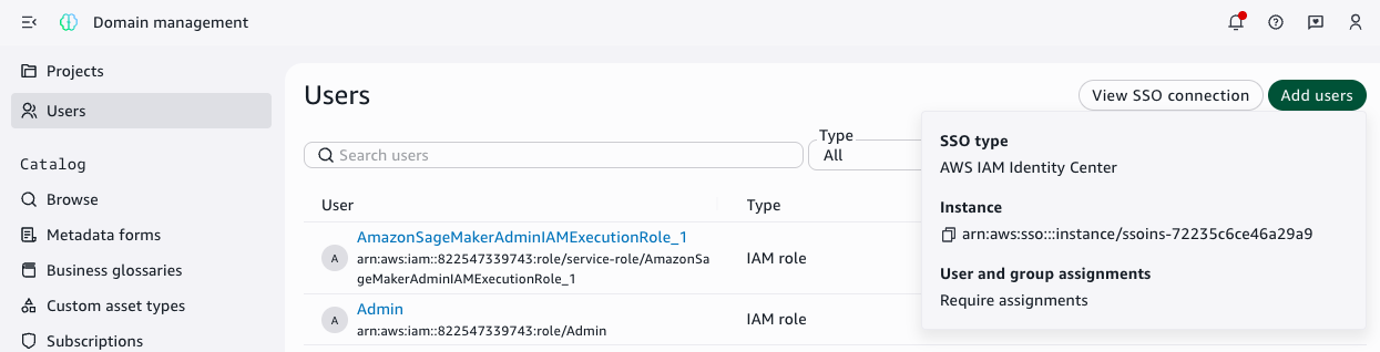
  4. Choose View SSO connection.
  5. Copy the end of the Instance ARN, so we can build the Instance URL like https://identitycenter.amazonaws.com/ssoins-0example

The following screenshot shows the Amazon SageMaker Unified Studio domain management page with SSO connection details.

SageMaker Unified Studio domain SSO connection details showing the IAM Identity Center instance ARN

Figure 5: AWS IAM Identity Center information

  1. Choose the user icon and copy the Region as shown in the following screenshot.
SageMaker Unified Studio user menu showing the Region

Figure 6: User icon with the Region information

Method 1: DSN-based connection (Athena Power BI connector)

In this method, you configure an ODBC Data Source Name (DSN) and use the Amazon Athena connector in Power BI. This method uses SageMakerIam authentication mode and supports both DirectQuery and Import mode.

This section covers IAM-based domains. For IDC-based domains, see Part 1.

Gather configuration values to configure your Amazon Athena ODBC DSN

Before configuring the ODBC DSN, gather the following connection values from your Amazon SageMaker Unified Studio project:

  1. Open your Amazon SageMaker Unified Studio Project.
  2. Top right, select the three dots.
  3. Choose Project details.
  4. Select JDBC and ODBC details.
  5. Copy the following values: domain ID, Amazon SageMaker project ID, AWS Region, and Athena workgroup.

The following screenshot shows the Amazon SageMaker Unified Studio project overview page, which provides the project details to copy.

SageMaker Unified Studio project details showing domain ID, project ID, Region, and Athena workgroup

Figure 7: Project details with SageMaker domain ID, SageMaker project ID, Region, and Athena workgroup

Configure the ODBC DSN

Create a System DSN using the Amazon Athena ODBC driver. For the general DSN creation steps, see Configuring a data source name on Windows in the Amazon Athena User Guide. Enter the following values:

Field Value
Data Source Name Name your datasource (for example, pbi-iamdomain)
Region The AWS Region where your Amazon SageMaker domain is provisioned (for example, us-east-1)
Catalog AwsDataCatalog
Database default
Workgroup Your Athena workgroup name (for example, workgroup-abcdefghij-klmexample)

In the Authentication Options, configure the following values:

Field Value
Authentication Type SageMakerIam
SageMaker Domain ID dzd-123456example
SageMaker Project ID abcd12example
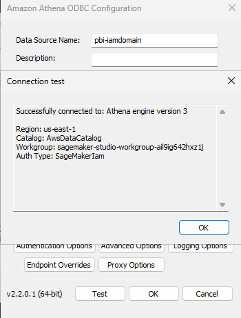
SageMaker Region Region of your SageMaker Unified Studio project (for example, us-east-1)

Choose OK, then Test to verify the connection. Choose Allow Access when prompted by the browser.

The following screenshot shows the successful connection test.

ODBC DSN configuration showing a successful connection test with SageMakerIam

Figure 8: Successful connection test in the ODBC DSN configuration with SageMakerIam authentication

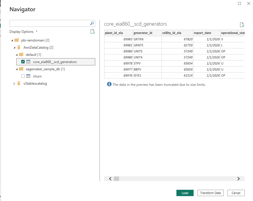
Connect Power BI Desktop to your data

With the DSN configured, you can connect Power BI Desktop to your data catalog and load the generators dataset.

  1. Open Microsoft Power BI Desktop.
  2. Open the Get Data menu and select More.
  3. Search for and select Amazon Athena and choose Connect.
  4. For Data Source Name (DSN), enter pbi-iamdomain.
  5. Select DirectQuery.
  6. Choose OK.
  7. Choose Use Data Source Configuration and then Connect.
  8. In the AwsDataCatalog folder, navigate to your database.
  9. Select the core_eia860__scd_generators table.
  10. Choose Load.

The following screenshot shows Power BI Desktop successfully connected to the data catalog.

Power BI Desktop connected to the data catalog with the generators table loaded

Figure 9: Power BI Desktop connected to the data catalog with the generators table loaded using SageMakerIam authentication

Create your dashboard and publish it

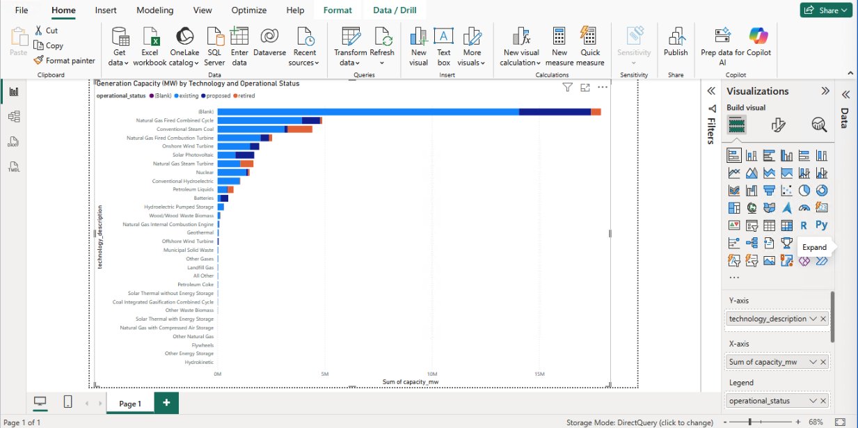
You can create a dashboard to visualize U.S. power generation data. To create a visualization, complete the following steps:

  1. In the Visualizations pane, choose the Stacked bar chart.
  2. Assign the Y-Axis: Drag technology_description to the Y-Axis.
  3. Assign the X-Axis (Values): Drag capacity_mw to the X-Axis (automatically summed).
  4. Assign the Legend (Stack): Drag operational_status to the Legend field.
  5. Choose Publish.
  6. Give your report a name (for example, generation-iamdomain) and choose Save.
  7. Sign in and choose a destination workspace.

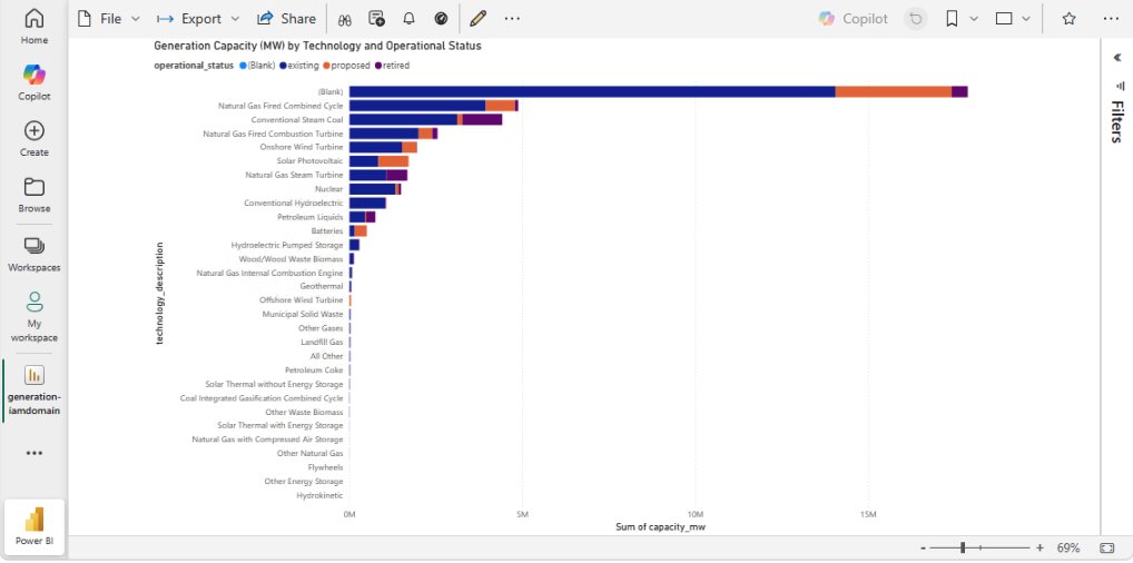
The following screenshot shows the Power BI dashboard with U.S. power generation data.

Power BI stacked bar chart of U.S. generation capacity by technology and operational status

Figure 10: Power BI dashboard with U.S. power generation data

After you publish, the report structure becomes available on Microsoft Power BI Service.

Method 2: DSN-less connection (Power BI ODBC connector)

In this method, you use the Power BI ODBC connector with a connection string (no DSN required). This method supports Import mode only and SageMakerIam authentication. Because the gateway can’t perform browser authentication and connection strings need to match, both Desktop and gateway must use SageMakerIam.

This section covers IAM-based domains. For IDC-based domains, see Part 1.

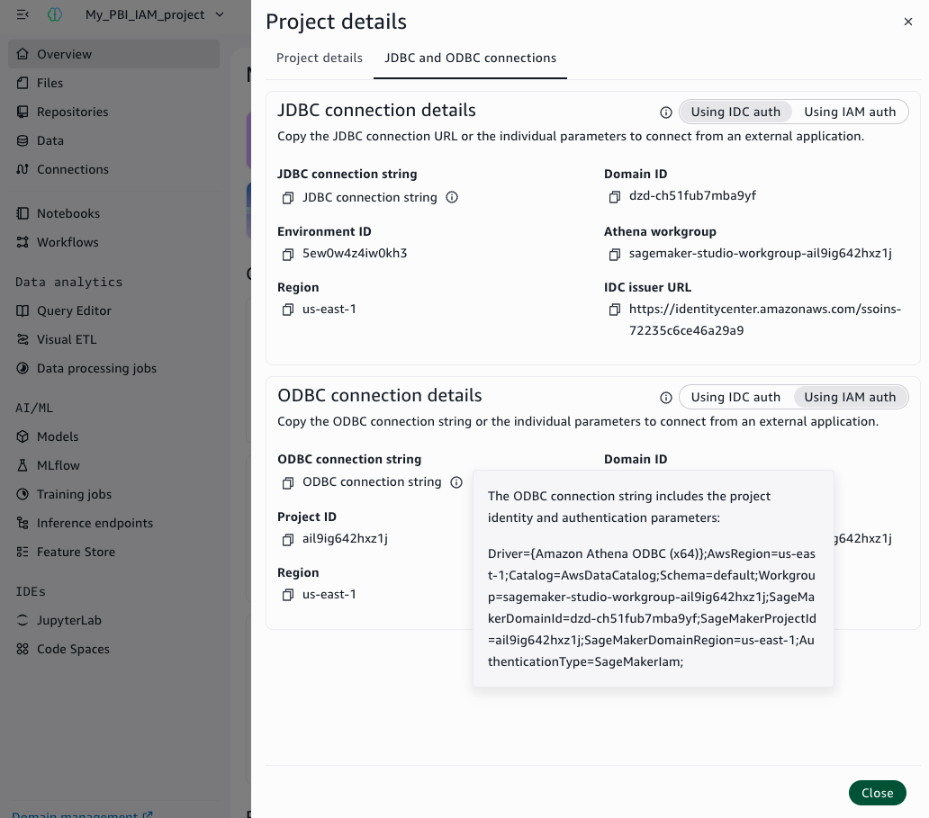
Gather configuration values to configure your DSN-less connection

Gather the following connection values from your Amazon SageMaker Unified Studio project:

  1. Open your Amazon SageMaker Unified Studio Project.
  2. Top right, select the three dots.
  3. Choose Project details.
  4. Select JDBC and ODBC details.
  5. Copy the ODBC connection string.

The following screenshot shows the Amazon SageMaker Unified Studio project overview page with the ODBC connection string to copy.

SageMaker Unified Studio project overview showing the ODBC connection string

Figure 11: Project details with ODBC connection string

Connect Power BI Desktop to your data and publish

With the configuration parameters of your project, you can connect Power BI Desktop to your data catalog and load the generators dataset.

  1. Open Power BI Desktop.
  2. Open the Get Data menu and select More.
  3. Search for and select ODBC and choose Connect.
  4. For Data Source Name (DSN), select (None).
  5. Expand Advanced Options.
  6. In the Connection string field, enter your connection string. For example, Driver={Amazon Athena ODBC (x64)};AwsRegion=us-east-1;Catalog=AwsDataCatalog;Schema=default;Workgroup=workgroup-abcdefghij-klmexample;SageMakerDomainId= dzd-123456example;SageMakerProjectId= abcd12example;SageMakerDomainRegion=us-east-1;AuthenticationType=SageMakerIam;
  7. Choose OK.
  8. Choose Default or Custom and then Connect.
  9. In the AwsDataCatalog folder, navigate to your database.
  10. Select the core_eia860__scd_generators table.
  11. Choose Load.

When publishing, name your report generation-iamdomain-dsnless.

Configure the gateway and view your report on Power BI Service

After creating your reports in Power BI Desktop, configure the on-premises data gateway to view your report on Power BI Service.

You can configure the gateway using either a DSN or a DSN-less connection string, matching the method you used in Power BI Desktop.

Create and attach an IAM role to the Power BI Gateway EC2 instance

Create an IAM role for the EC2 instance that will host your Power BI gateway. Name the role pbi-gateway-role (or a name of your choice). The role must use EC2 as the trusted entity and include the following inline policy:

{
    "Version": "2012-10-17",
    "Statement": [
        {
            "Sid": "SageMakerAccess",
            "Effect": "Allow",
            "Action": [
                "datazone:GetConnection",
                "datazone:ListConnections",
                "datazone:GetDomain",
                "datazone:GetProject"
            ],
            "Resource": "*"
        },
        {
            "Sid": "STSForDriver",
            "Effect": "Allow",
            "Action": [
                "sts:GetCallerIdentity"
            ],
            "Resource": "*"
        }
    ]
}

Attach this role to your Power BI Gateway EC2 instance. For detailed steps on creating and attaching an IAM role to an EC2 instance, refer to IAM roles for Amazon EC2 in the Amazon EC2 User Guide.

Add the Power BI Gateway IAM role as a member of SageMaker Unified Studio project

The gateway IAM role needs project-level access to query data through Athena. The steps to add the role differ depending on your domain type.

IAM-based domain

  1. Open your Amazon SageMaker Unified Studio Project.
  2. Open Domain Management.
  3. Choose your Project Name.
  4. Choose Members.
  5. Choose Add members.
  6. Select the IAM role of your Power BI gateway (for example, pbi-gateway-role).
  7. Choose Add.

The following screenshot shows the Amazon SageMaker Unified Studio project domain management page with options to add members to a project.

SageMaker Unified Studio project members list including the Power BI gateway IAM role

Figure 12: List of members of a SageMaker Unified Studio project with the IAM gateway role

Configure the data source on Power BI Gateway

How you configure the data source depends on the method you used in Power BI Desktop.

Method 1 (DSN-based)

Configure a System DSN on the gateway EC2 instance following the same ODBC DSN steps described in Method 1. When configuring, make sure that:

  • You use the System DSN tab (not User DSN) because the gateway runs as a Windows service under a separate account.
  • The authentication type is set to SageMakerIam.
  • The DSN name matches exactly the one configured on Power BI Desktop (for example, pbi-iamdomain).

Method 2 (DSN-less)

No configuration is needed on the gateway machine itself. You configure the data source directly in Power BI Service.

Configure the data source and view your report on Power BI Service

To view your report, complete the following steps:

  1. Open the workspace where you saved your report.
  2. Search the Semantic Model which has the same name as your report (for example, generation-iamdomain) and choose the More options icon (three dots).
  3. Choose Settings.
  4. Expand Gateway and Cloud Connection.
  5. Choose View Datasources (play icon) on your gateway.
  6. Choose Manually add to gateway.
  7. Add a connection name (for example, pbi-iamdomain).

The next step depends on the method that you chose:

Method 1 (DSN-based)

  1. Add the DSN (for example, pbi-iamdomain) that matches exactly the one configured on Power BI Desktop.

Method 2 (DSN-less)

  1. In the Connection string field, enter the connection string that matches exactly the one used in Power BI Desktop.

Next, continue with the configuration:

  1. Select Anonymous as Authentication Method.
  2. Choose Create.
  3. Expand again Gateway and Cloud Connection.
  4. For Maps to, choose the connection that you created (for example, pbi-iamdomain).
  5. Choose Apply.
  6. Return to the workspace where you saved your report.
  7. On the Content section, choose your report (for example, generation-iamdomain).

The following screenshot shows a report on Power BI Service.

Published Power BI report rendering on Power BI Service

Figure 13: Power BI report on Power BI Service

You can now see your report online with the data from your Amazon SageMaker Unified Studio project.

Clean up

To avoid additional charges after testing, delete the Amazon SageMaker Unified Studio domain and EC2 instances. Refer to Delete domains and Terminate Instances for instructions.

Conclusion

In this two-part series, you connected Power BI to Amazon SageMaker Unified Studio through Amazon Athena. Part 1 covered IDC-based domains. This post covered IAM-based domains using SageMakerIam authentication. This provides a direct connection path, with no third-party licensing, while maintaining data governance and security.

You can automate many steps of this process. For information about automating DSN creation on the Power BI Gateway or Service, refer to How ENGIE automates the deployment of Amazon Athena data sources on Microsoft Power BI. If you don’t want users adding the gateway IAM role directly, you can create a custom blueprint as a self-service tool for gateway role addition. The blueprint uses a ProjectMembership resource with a configurable parameter that project owners can activate at project creation, automatically adding the gateway role as a project contributor.

For additional best practices, refer to the Using Microsoft Power BI with the AWS Cloud Whitepaper. To learn more, visit Amazon SageMaker Unified Studio and Amazon Athena.


About the authors

Ramesh H Singh

Ramesh H Singh

Ramesh is a Senior Product Manager Technical at AWS in Seattle, focused on Amazon SageMaker. He’s passionate about building analytics and AI products that help enterprise customers unlock real value from their data. Away from work, he spends his time hiking with family and exploring spirituality. Connect with him on LinkedIn.

Armando Segnini

Armando Segnini

Armando is a Senior Analytics Specialist Solutions Architect at AWS, partnering with enterprise customers to architect scalable data, analytics, and AI platforms. He helps organizations turn complex data challenges into business value through expertise in streaming, BI integration, and generative AI. Outside of work, Armando enjoys traveling with his family, exploring new cultures, photography, and functional fitness competitions.

Gaurav Sharma

Gaurav is a Specialist Solutions Architect (Analytics) at AWS, supporting US public sector customers on their cloud journey. Outside of work, Gaurav enjoys spending time with his family and reading books.

Krishna Atluru

Krishna Atluru

Krishna is an Enterprise Support Lead TAM at AWS. He provides customers with in-depth guidance on improving security posture and operational excellence for their workloads, helping them build secure, resilient, and cost-effective solutions. His areas of expertise include building serverless architectures, and data and analytics solutions. Outside of work, Krishna enjoys cooking, swimming, and traveling.

Saushthav Saxena

Saushthav Saxena

Saushthav is a Software Development Engineer at AWS on the Amazon Athena team, where he has spent the past few years working on distributed systems and data analytics at scale. Based in the San Francisco Bay Area, his background spans full-stack development, high-performance computing, and large-scale infrastructure. Outside of work, he enjoys reading sci-fi novels, swimming, and traveling with family and friends.

Track SageMaker Unified Studio project costs with custom tags and AWS CUR

Post Syndicated from Nisha Gambhir original https://aws.amazon.com/blogs/big-data/track-sagemaker-unified-studio-project-costs-with-custom-tags-and-aws-cur/

Organizations running machine learning (ML), analytics, and generative AI workloads on Amazon SageMaker Unified Studio domains and projects face a common cost governance challenge. System tags (AmazonDataZoneDomainId and AmazonDataZoneProject) are automatically propagated to all underlying project resources. However, custom tags such as CostCenter, Team, or Environment are not propagated to dynamic resources created through the Studio UI. This creates a gap when you need to report project costs grouped by custom tags.

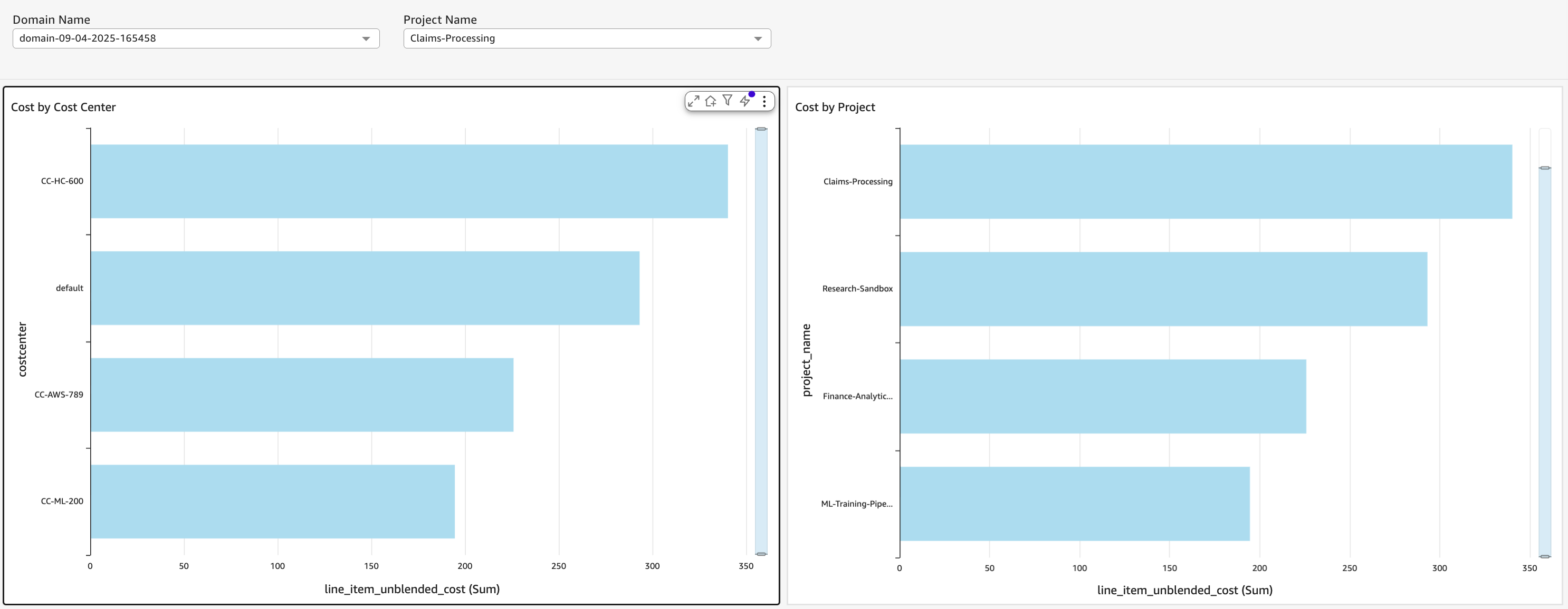
In this post, we walk through a serverless solution that bridges this gap by enriching AWS Cost and Usage Report (CUR) data with custom project tags. By the end of this post, you can build an Amazon Quick Sight dashboard to filter and analyze Amazon SageMaker Unified Studio project costs by any custom tag dimension that you define. This gives your team the visibility to make informed spending decisions.

Solution overview

The solution consists of three automated subsystems:

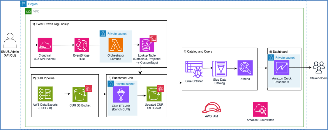
  1. Event-driven tag lookup management – An Amazon EventBridge rule captures Amazon DataZone project lifecycle events (Create, Update, Delete) and triggers an AWS Lambda function. The function maintains an Amazon DynamoDB lookup table that maps each project’s DomainId and ProjectId to its custom tags.
  2. CUR enrichment pipeline – An AWS Glue extract, transform, and load (ETL) job reads CUR 2.0 Parquet data from Amazon Simple Storage Service (Amazon S3). The job joins each billing line item with the DynamoDB lookup table using the system tags (DomainId, ProjectId), appends the custom tag values as new columns, and writes the enriched data back to Amazon S3.
  3. Cost visualization – An Amazon Quick Sight dashboard backed by a custom SQL dataset over Amazon Athena provides interactive cost and consumption analytics filtered by custom tags.

Architecture

The following diagram shows the end-to-end architecture:

Figure 1: SageMaker Unified Studio project custom tag cost reporting

The workflow is as follows:

  • An Amazon SageMaker Unified Studio administrator creates or updates a project with custom tags.
  • AWS CloudTrail captures the API call.
  • Amazon EventBridge matches the event.
  • The Lambda orchestrator writes the tag mapping to DynamoDB.
  • Separately, AWS Data Exports delivers CUR data to Amazon S3.
  • The AWS Glue ETL job enriches CUR line items with custom tags from DynamoDB.
  • The AWS Glue Crawler catalogs the enriched data.
  • Amazon Quick Sight visualizes costs by custom tags.

Prerequisites

Before deploying this solution, you need:

  • An Amazon SageMaker Unified Studio domain (you create projects after deployment).
  • AWS Cloud Development Kit (AWS CDK) CLI installed.
  • Python 3.12+.
  • Amazon Quick Sight Enterprise edition enabled in your account.
  • An AWS Identity and Access Management (IAM) user or role with permissions to deploy AWS CloudFormation stacks.

Step 1: Configure custom tags on your project profile

You configure custom tags on project profiles through the Amazon DataZone API. First, enable custom tags on your project profile:

aws datazone update-project-profile \
  --domain-identifier $DOMAIN_ID \
  --identifier $PROJECT_PROFILE_ID \
  --region $REGION \
  --allow-custom-project-resource-tags \
  --project-resource-tags '[
  {"key": "CostCenter", "value": "default", "isValueEditable": true},
  {"key": "Team", "value": "default", "isValueEditable": true},
  {"key": "Environment", "value": "default", "isValueEditable": true}
]'

When creating or updating a project, set the tag values:

aws datazone update-project \
  --domain-identifier $DOMAIN_ID \
  --identifier $PROJECT_ID \
  --project-profile-version latest \
  --region $REGION \
  --resource-tags '{"CostCenter": "CC-100", "Team": "ML-Platform", "Environment": "Production"}'

Important: The AmazonSageMakerProvisioning-<domainAccountId> role needs an inline policy that permits your custom tag keys. Without this, project environment deployment fails.

The following is the inline policy that’s used for the custom tags shared in this post:

{
  "Version": "2012-10-17",
  "Statement": [
    {
      "Sid": "AllowCustomTagKeys",
      "Effect": "Allow",
      "Action": [
        "sagemaker:AddTags",
        "sagemaker:DeleteTags",
        "cloudformation:TagResource",
        "cloudformation:CreateStack",
        "cloudformation:UpdateStack"
      ],
      "Resource": "*",
      "Condition": {
        "ForAnyValue:StringLike": {
          "aws:TagKeys": [
            "AmazonDataZone*",
            "CostCenter",
            "Team",
            "Environment"
          ]
        }
      }
    }
  ]
}

Step 2: Activate cost allocation tags

Activate the SageMaker Unified Studio system tags as cost allocation tags so they appear in CUR data:

aws ce update-cost-allocation-tags-status \
  --cost-allocation-tags-status '[
  {"TagKey": "AWSDataZoneProject", "Status": "Active"},
  {"TagKey": "AmazonDataZoneDomainId", "Status": "Active"}
]'

These tags take up to 24 hours to start appearing in CUR reports after activation.

Step 3: Deploy the infrastructure

The solution is packaged as a CDK application. Clone the GitHub repository and deploy:

# Install dependencies
pip install -r requirements.txt

# Bootstrap CDK (first time only)
cdk bootstrap aws://$ACCOUNT_ID/$REGION

# Deploy
cdk deploy

This creates the following resources:

  • DynamoDB table (smus-project-tag-lookup) – stores project-to-tag mappings.
  • Lambda function (smus-orchestrator) – processes project lifecycle events.
  • Amazon EventBridge rule – matches Amazon DataZone CreateProject/UpdateProject/DeleteProject events.
  • S3 buckets – for raw CUR and enriched CUR data.
  • AWS Glue ETL job (smus-cur-enrichment) – enriches CUR with custom tags.
  • AWS Glue Crawler – catalogs enriched data.
  • Amazon Simple Notification Service (Amazon SNS) topic – pipeline failure alerts.

Note: The solution uses serverless components (Lambda, DynamoDB on-demand, AWS Glue, Amazon Quick Sight), so you only pay for what you use. The primary cost drivers are AWS Glue ETL job execution time and Amazon Quick Sight SPICE storage.

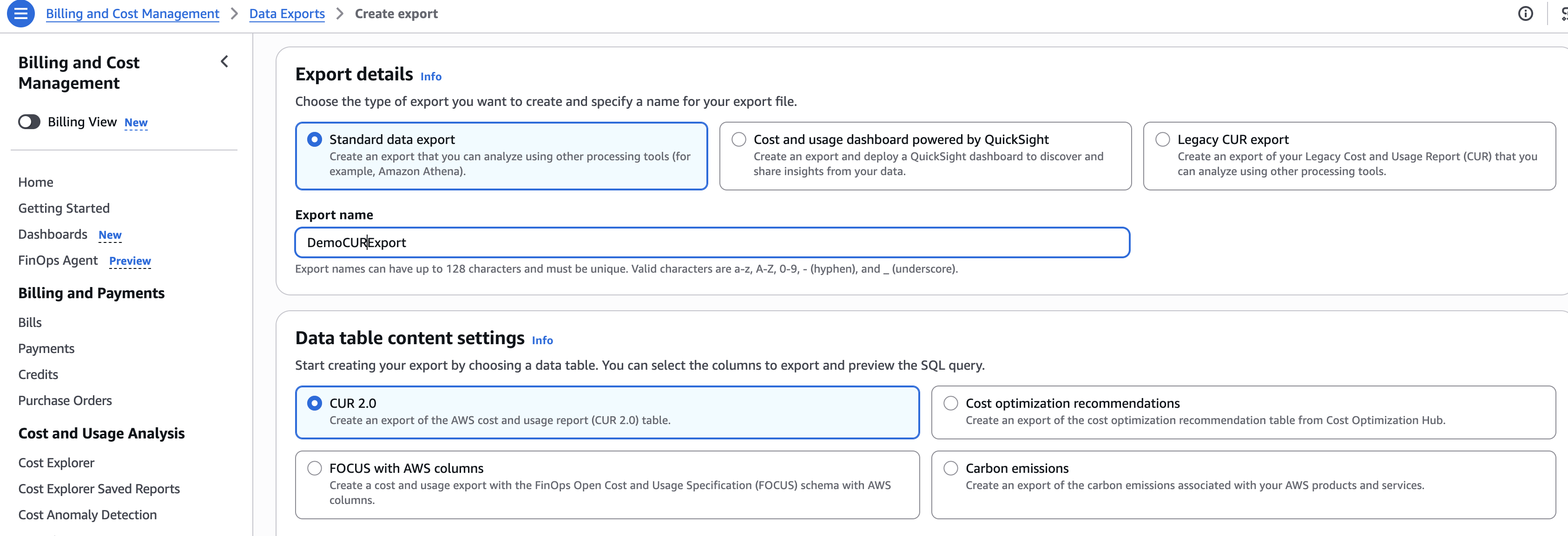
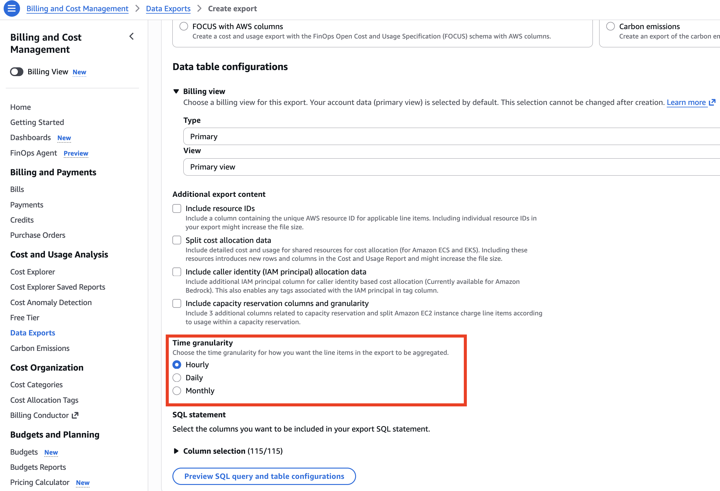
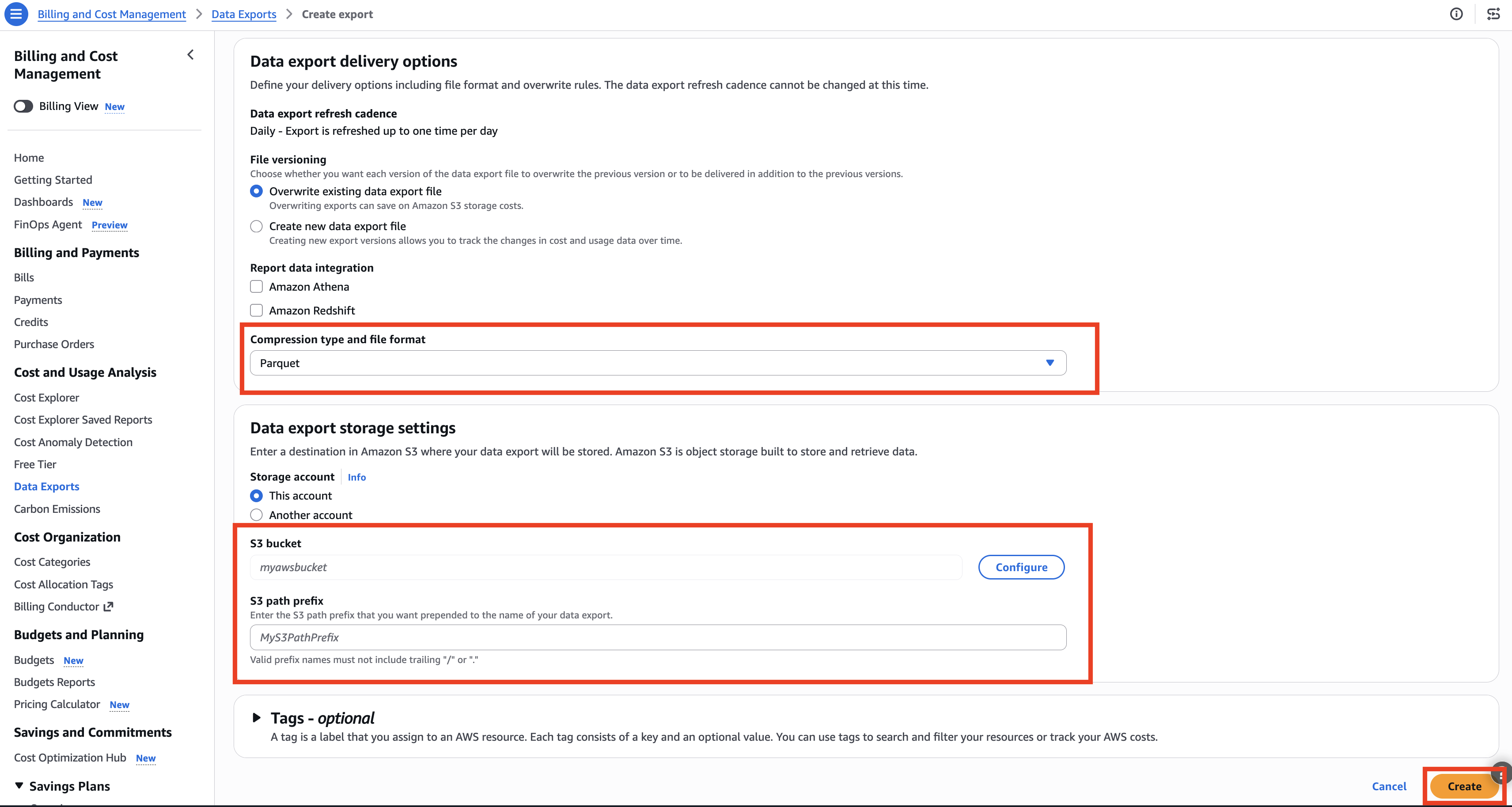
Step 4: Configure CUR delivery

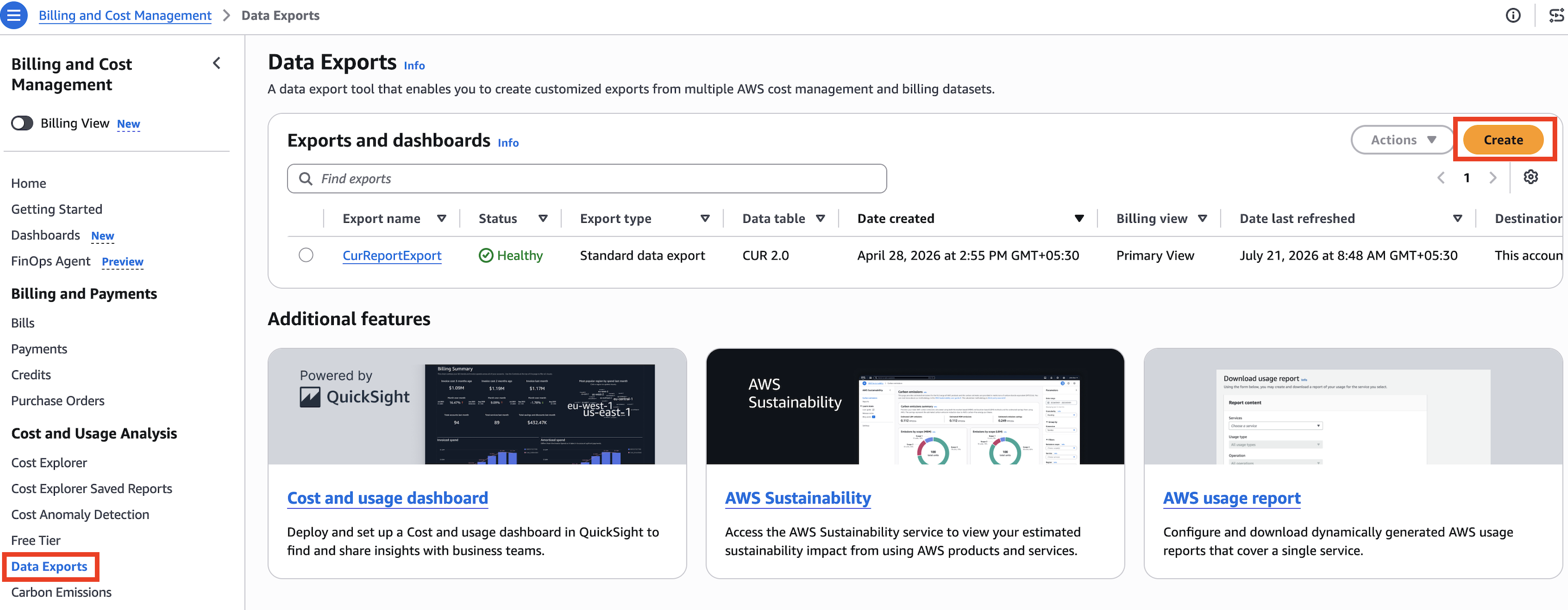
Create a CUR 2.0 export through AWS Data Exports that delivers Parquet files to the CUR S3 bucket created by the stack. The following screenshots show the complete configuration process in the AWS Billing and Cost Management console.

To create the export, follow these steps:

  1. Go to AWS Billing and Cost Management and then choose Data Exports.
  2. Choose Create in the upper right corner of the Exports and dashboards page. The Data Exports console shows any existing exports, their status, export type, data table, and last refresh date.
  3. On the Create export page, under Export details, select Standard data export and enter an export name. Under Data table content settings, select CUR 2.0.
  4. Under Data table configurations, set Time granularity to Hourly. The configuration page also lets you choose additional export content options such as including resource IDs, split cost allocation data, caller identity allocation data, and capacity reservation columns.
  5. Under Data export delivery options, set Compression type and file format to Parquet. Under Data export storage settings, configure the S3 bucket to: smus-cur-report-{account-id}-{region} and set the S3 path prefix as needed. Choose Create to finish.
Data Exports console listing existing exports with status, type, and last refresh date

Figure 2: Data Exports page listing existing exports

Create export page with Standard data export selected and CUR 2.0 chosen

Figure 3: Create export page with Standard data export and CUR 2.0 selected

Data table configurations with time granularity set to Hourly

Figure 4: Data table configurations with time granularity set to Hourly

Data export delivery options with Parquet format and the S3 storage destination configured

Figure 5: Data export delivery options with Parquet format and S3 storage settings

Step 5: How the event-driven tag capture works

When a project is created or updated in Amazon SageMaker Unified Studio (through the Studio UI or API), the following happens automatically:

  1. CloudTrail logs the Amazon DataZone API call.
  2. Amazon EventBridge matches the event.
  3. Amazon EventBridge invokes the Lambda function.
  4. The Lambda extracts custom tags from the CloudTrail event payload.
  5. The Lambda writes a record to DynamoDB with the DomainId, ProjectId, and all custom tag key-value pairs.

The Lambda function reads tags directly from the responseElements.resourceTags field of the CloudTrail event rather than making a separate GetProject API call. This avoids a race condition where GetProject might return empty tags while the project is in the UPDATING state.

def _extract_tags_from_event(detail):
    tags = {}
    response_elements = detail.get("responseElements") or {}
    for tag_entry in response_elements.get("resourceTags", []):
        if isinstance(tag_entry, dict) and "key" in tag_entry:
            tags[tag_entry["key"]] = tag_entry["value"]
    request_params = detail.get("requestParameters") or {}
    req_tags = request_params.get("resourceTags", {})
    if isinstance(req_tags, dict):
        tags.update(req_tags)
    return tags

Step 6: How the CUR enrichment works

The AWS Glue ETL job runs on a schedule (after each CUR delivery):

  1. Reads CUR Parquet files from the CUR S3 bucket.
  2. Reads all records from the DynamoDB lookup table.
  3. Performs a left outer join on DomainId and ProjectId.
  4. Appends custom tag columns (CostCenter, Team, Environment, and so on) to each CUR line item.
  5. Writes enriched Parquet to the enriched S3 bucket.

Line items without a matching project in the lookup table retain all original columns with NULL custom tag values. No data is dropped.

joined_df = cur_df.join(
    lookup_df,
    on=(
        (cur_df[DOMAIN_COL] == lookup_df["domainId"])
        & (cur_df[PROJECT_COL] == lookup_df["projectId"])
    ),
    how="left_outer",
)

Step 7: Set up the Amazon Quick Sight dashboard

After the first ETL run and crawler execution, set up the Amazon Quick Sight dashboard:

python scripts/setup_quicksight.py \
  --account-id $ACCOUNT_ID \
  --region $REGION \
  --quicksight-user $QUICKSIGHT_USER_ARN

This creates a dashboard with five visuals:

  • Cost by Custom Tag (CostCenter) – horizontal bar chart.
  • Cost by Project – horizontal bar chart.
  • Daily Cost Trend – line chart.
  • Cost by Service per Project – stacked bar chart.
  • Usage by Project & Service – summary table.

And six interactive list filters: Domain, Project, CostCenter, Team, Environment, Service.

The custom SQL includes a CASE statement for service categorization:

SELECT
  line_item_usage_start_date,
  line_item_product_code,
  line_item_usage_amount,
  line_item_unblended_cost,
  resource_tags_user_amazondatazone_domain_id AS domain_id,
  resource_tags_user_amazondatazone_project AS project_id,
  costcenter, team, environment,
  CASE
    WHEN line_item_product_code = 'AmazonSageMaker' THEN 'SageMaker'
    WHEN line_item_product_code = 'AmazonS3' THEN 'S3'
    WHEN line_item_product_code = 'AWSGlue' THEN 'Glue'
    ELSE line_item_product_code
  END AS service_category
FROM "smus_cost_reporting"."enriched_cur"
WHERE line_item_unblended_cost > 0

Step 8: Verifying the solution

After deploying the infrastructure and setting up the dashboard, verify that each component of the pipeline is functioning correctly.

8.1 Verify Amazon EventBridge is capturing project events

  1. Open the Amazon EventBridge console.
  2. In the navigation pane, choose Rules.
  3. Select the rule created by the CDK stack (for example, SmusCostReporting-ProjectTagRule).
  4. Choose the Monitoring tab.
  5. Confirm that the invocations are being recorded in the metrics.
  6. Create or update an Amazon SageMaker Unified Studio project with custom tags using the following command:
    aws datazone update-project \
      --domain-identifier <domain-id> \
      --identifier <project-id> \
      --custom-tags CostCenter=Engineering Team=DataPlatform Environment=Production

  7. Within a few seconds, the Amazon EventBridge rule should show a new invocation in its metrics.

8.2 Verify DynamoDB schema and tag mappings

The DynamoDB lookup table uses a simple key schema:

Attribute Type Role
domainId String Partition Key
projectId String Sort Key
CostCenter String Custom tag
Team String Custom tag
Environment String Custom tag

Custom tags are stored as dynamic attributes. Any tag key set on a project becomes a column in the table.

8.2.1 Verify DynamoDB table contains tag mappings

  1. Open the DynamoDB console.
  2. Navigate to the table created by the stack (for example, SmusCostReporting-ProjectTagsTable).
  3. Choose Explore table items.
  4. Scan for your project with the following keys:
    Partition key (domainId): <your-domain-id>
    Sort key (projectId): <your-project-id>

  5. Confirm the item contains the expected custom tag attributes (CostCenter, Team, Environment) with the values you assigned.
  6. Alternatively, use the AWS CLI:
    aws dynamodb get-item \
      --table-name SmusCostReporting-ProjectTagsTable \
      --key '{"domainId": {"S": "<domain-id>"}, "projectId": {"S": "<project-id>"}}'

8.3 Verify the AWS Glue ETL job enriches CUR data

  1. Wait for the next CUR delivery (hourly if configured as described in Step 4).
  2. Wait for the subsequent AWS Glue job execution.
  3. Open the AWS Glue console.
  4. In the navigation pane, choose ETL Jobs.
  5. Confirm the job completed successfully (status: Succeeded).
  6. Query the enriched data in Amazon Athena to confirm custom tag columns are populated:
    SELECT
      line_item_usage_start_date,
      line_item_product_code,
      line_item_unblended_cost,
      costcenter,
      team,
      environment
    FROM "smus_cost_reporting"."enriched_cur"
    WHERE costcenter IS NOT NULL
    LIMIT 10;

You should see rows with your custom tag values populated in the costcenter, team, and environment columns.

8.4 Verify the Amazon Quick Sight dashboard displays enriched data

  1. Open the Amazon Quick Sight console and navigate to the dashboard created by the setup script.
  2. Confirm that:
    • The Cost by Custom Tag (CostCenter) bar chart displays cost data grouped by your CostCenter values.
    • The list filters for CostCenter, Team, and Environment contain selectable values.
    • Selecting a filter value correctly narrows the displayed data.
  3. If the dashboard shows no data, verify that:
    • The AWS Glue Crawler has run after the ETL job (check the crawler’s last run status in the AWS Glue console).
    • The SPICE dataset has been refreshed. In the Amazon Quick Sight console, navigate to Datasets, select the dataset, and then choose Refresh now.

Figure 6 shows the Amazon Quick Sight dashboard with two side-by-side horizontal bar charts: Cost by Cost Center and Cost by Project. Domain Name and Project Name list filters appear at the top.

Amazon Quick Sight dashboard with Cost by Cost Center and Cost by Project bar charts and Domain and Project filters

Figure 6: Amazon Quick Sight dashboard showing cost data by custom tags, including Cost by Cost Center and Cost by Project bar charts with Domain Name and Project Name filters

Note: The first end-to-end cycle can take up to 48 hours depending on CUR delivery timing. After the initial cycle completes, subsequent updates will flow automatically on the configured schedule.

Operational considerations

Monitoring: The Amazon SNS topic smus-cost-reporting-alerts receives notifications when the AWS Glue ETL job fails or the Lambda orchestrator encounters repeated errors. Subscribe an email address or Slack webhook to stay informed. For instructions on how to create a subscription, see Subscribing to an Amazon SNS topic.

Cost: The solution uses serverless components (Lambda, DynamoDB on-demand, AWS Glue, Amazon Quick Sight, SPICE) so you only pay for what you use. The primary cost drivers are AWS Glue ETL job execution time and Amazon Quick Sight SPICE storage.

Scaling: The DynamoDB table uses on-demand capacity and can scale to accommodate your projects. You can scale the AWS Glue ETL job by increasing the number of workers for larger CUR datasets. For more information, see Managing throughput capacity automatically with DynamoDB auto scaling.

New tag keys: When you add new custom tag keys to projects, the ETL automatically picks them up as new columns. The AWS Glue Crawler’s UPDATE_IN_DATABASE policy adds new columns to the catalog table without manual intervention.

Cleanup

Warning: The following cleanup steps will permanently delete all CUR data, project tag mappings, and Amazon Quick Sight dashboards.

To remove all resources:

# Delete Amazon Quick Sight resources
python scripts/setup_quicksight.py --account-id $ACCOUNT_ID --region $REGION --quicksight-user $QS_USER --clean

# Delete CDK stack
cdk destroy

Go to AWS Billing and Cost Management, and then choose Data Exports and delete the CUR 2.0 export created in Step 4.

Deactivate the cost allocation tags that were activated in Step 2:

aws ce update-cost-allocation-tags-status \
  --cost-allocation-tags-status '[
  {"TagKey": "AWSDataZoneProject", "Status": "Inactive"},
  {"TagKey": "AmazonDataZoneDomainId", "Status": "Inactive"}
]'

Conclusion

In this post, we showed how to build an end-to-end cost reporting solution for Amazon SageMaker Unified Studio projects using custom tags. This solution combines tag capture driven by Amazon EventBridge, CUR enrichment through AWS Glue ETL, and visualization in Amazon Quick Sight. With it, organizations can track and attribute costs by CostCenter, Team, Environment, or any custom dimension. This works even for resources created through the Studio UI that don’t receive custom tag propagation.

This solution serves as an extension to the custom tag propagation feature and reports cost for all project resources. The architecture is fully serverless, automated, and can be deployed to any AWS account using the provided CDK application.

To start building your custom tag cost reporting pipeline, visit the GitHub repository. To learn more about the underlying services, visit the Amazon SageMaker Unified Studio service page. For a related approach to custom tag governance, see Use Amazon SageMaker custom tags for project resource governance and cost tracking

References


About the authors

Nisha Gambhir

Nisha Gambhir

Nisha is a Senior AI/ML & Cloud Architect based out of India. She is passionate about helping customers design, architect and develop secure, scalable and reliable applications using AI/ML and Agentic AI. She loves working on latest technologies, providing simple and scalable solutions that drive positive business outcomes.

Dr Anil Giri

Dr Anil Giri

Anil is a Solutions Architect at AWS, based in London, UK, where he helps ISV customers design and deploy agentic AI systems in production. He specializes in multi-agent orchestration, retrieval-augmented generation, and event-driven serverless architectures on Amazon Bedrock, with a focus on building reliable, secure, and scalable solutions that deliver measurable business outcomes.

Satish Sarapuri

Satish Sarapuri

Satish is a Sr. Data Architect, Data Mesh / Data Lake/Gen AI at AWS. He helps enterprise-level customers build high-performance, highly available, cost-effective, resilient, and secure generative AI, data mesh, data lake, and analytics platform solutions on AWS, through which customers can make data-driven decisions to gain impactful outcomes for their business and help them on their digital and data transformation journey. In his spare time, he enjoys trail running and spending quality time with his family.

Ram Vittal

Ram Vittal

Ram is a Principal GenAI/ML Specialist at AWS. He has over 3 decades of experience building distributed, hybrid, and cloud applications. He is passionate about building secure, scalable, reliable AI/ML and big data solutions to help customers with their cloud adoption and optimization journey. In his spare time, he rides motorcycle and enjoys the nature with his family.

Secure SageMaker Unified Studio access with SAML and conditional policies

Post Syndicated from Manos Samatas original https://aws.amazon.com/blogs/big-data/secure-sagemaker-unified-studio-access-with-saml-and-conditional-policies/

Amazon SageMaker Unified Studio is a single data and AI development environment that brings together data preparation, analytics, and machine learning (ML) development in one place. By unifying these workflows, it saves teams from managing multiple tools and makes it straightforward for data scientists, analysts, and developers to build, train, and deploy ML models while collaborating. In Amazon SageMaker Unified Studio, a domain is the organizing entity for connecting your assets, users, and their projects. With Amazon SageMaker unified domains, you have the flexibility to reflect the data and analytics needs of your organizational structure. You can create a single unified domain for your enterprise or multiple domains for different business units.

Some enterprises, especially those in regulated industries, might require limiting access to trusted networks (such as VPN CIDRs) or to managed devices that meet compliance standards through device attestation.

In this post, we demonstrate how to integrate SageMaker Unified Studio as a custom SAML application and apply conditional access policies for enforcing device compliance, IP-based restrictions, or multi-factor authentication (MFA). For this post, we use Okta as the identity provider (IdP).

Solution overview

This solution demonstrates how to integrate Amazon SageMaker Unified Studio (SMUS) with external SAML identity providers such as Okta. The integration enforces enterprise security controls, including trusted network access, device compliance, and multi-factor authentication. With this integration, organizations in regulated industries can maintain strict access controls while providing single sign-on for their data science and AI development teams. By using SAML 2.0 federation with conditional access policies, you can help make sure that only authenticated users on compliant devices from trusted networks gain access. This access applies to your SageMaker Unified Studio domains and the associated data and AI workloads.

SAML authentication flow from a corporate device through the identity provider and AWS STS to Amazon SageMaker Unified Studio

Authentication flow for accessing SageMaker Unified Studio through SAML

The architecture diagram illustrates the secure authentication flow for accessing SageMaker Unified Studio through SAML integration:

  1. Users typically initiate access from corporate-managed devices through VPN or trusted network connections.
  2. The IdP authenticates the user and evaluates conditional access policies defined by your organization. Based on these policies, it checks for trusted devices, approved source IP ranges, and MFA completion. If any policy fails, the login is rejected. Otherwise, authentication proceeds.
  3. Upon successful authentication and policy validation, the IdP generates a digitally signed SAML assertion containing user attributes and group memberships, securely delivering it to the user’s browser through HTTP POST binding.
  4. The client browser automatically posts the SAML assertion to the AWS Security Token Service (AWS STS) sign-in endpoint. There, the AWS IAM Identity Provider validates the trust relationship with your corporate IdP through pre-configured SAML federation settings.
  5. AWS STS validates the SAML assertion signature and authenticity. It then maps the user attributes to a specifically configured IAM role with SageMaker Unified Studio permissions, including the datazone:GetIamPortalLoginUrl permission required for domain access.
  6. AWS STS confirms successful role assumption and generates temporary AWS credentials with a defined session duration. It then issues an HTTP redirect that returns the browser to the SageMaker Unified Studio domain with authenticated session tokens.
  7. Users gain access to the unified environment for data preparation, analytics, and machine learning development. All activities are governed by the assumed IAM role permissions and logged for comprehensive audit trails.

Walkthrough

In this walkthrough, you create a SAML application in Okta, connect it to AWS, and configure a SageMaker Unified Studio domain to use it for authentication.

Prerequisites

Before you get started, make sure you have the following:

  1. Familiarity with Amazon SageMaker Unified Studio.
  2. A basic understanding of SAML 2.0.
  3. AWS Identity and Access Management (IAM) permissions to create a domain in Amazon SageMaker Unified Studio.
  4. Access to your SAML IdP (such as Okta or Entra ID) to create and configure a SAML application.

Step 1: Create an application in Okta

The first step is to set up a new SAML application in Okta that manages authentication for SMUS.

  1. In Okta, go to ApplicationsCreate App Integration, and choose SAML 2.0.
  2. Provide an App name.
  3. Set the Single sign-on URL to https://signin.aws.amazon.com/saml.
  4. Set Name ID format to Persistent.
  5. Set the Audience URI (SP Entity ID) to https://signin.aws.amazon.com/saml.
  6. Choose Next, and finish creating the application.
  7. Once created, copy the Metadata URL and Sign On URL. You need these in later steps.

Step 2: Create an identity provider in IAM

Now, let’s connect Okta to AWS by creating an IAM identity provider. This allows AWS to trust authentication responses from Okta.

  1. Open the IAM console.
  2. Go to Identity providersAdd provider.
  3. Select SAML as the provider type.
  4. Provide a Provider name.
  5. In Okta, go to your application’s Sign On tab, choose Identity Provider metadata, and save the XML file. Upload it here.
  6. Choose Add provider.
  7. Copy the ARN of this provider. You need it when you create the role.

Step 3: Create an IAM role for Okta

Next, create an IAM role that Okta can assume. This role defines what access users have when they sign in through Okta.

  1. In IAM, go to RolesCreate role.
  2. Use the following trust policy (replace both instances of “{Replace with Identity provider ARN}” with the ARN you copied in Step 2):
{
    "Version": "2012-10-17",
    "Statement": [
        {
            "Effect": "Allow",
            "Principal": {
                "Federated": "{Replace with Identity provider ARN}"
            },
            "Action": "sts:AssumeRoleWithSAML",
            "Condition": {
                "StringEquals": {
                    "SAML:aud": "https://signin.aws.amazon.com/saml"
                }
            }
        },
        {
            "Effect": "Allow",
            "Principal": {
                "Federated": "{Replace with Identity provider ARN}"
            },
            "Action": "sts:TagSession",
            "Condition": {
                "StringLike": {
                    "aws:RequestTag/Email": "*"
                }
            }
        }
    ]
}
  1. Attach a permission policy. For example:
{
    "Version": "2012-10-17",
    "Statement": [
        {
            "Sid": "VisualEditor0",
            "Effect": "Allow",
            "Action": "datazone:GetIamPortalLoginUrl",
            "Resource": "arn:aws:datazone:<REGION>:<ACCOUNT-ID>:domain/<DOMAIN-ID>"
        }
    ]
}

Replace <REGION>, <ACCOUNT-ID>, and <DOMAIN-ID> with the corresponding values from your SageMaker Unified Studio domain ARN (arn:aws:sagemaker:<REGION>:<ACCOUNT-ID>:domain/<DOMAIN-ID>). You can find the domain ARN in the SageMaker console under Domains.

Step 4: Configure SAML assertions

To make sure AWS understands who is signing in, configure the SAML assertions in Okta.

  1. Open your application in Okta.
  2. Go to GeneralSAML SettingsEdit.
  3. Choose Next until you reach Attribute Statements.
  4. Add the following mappings:
    • https://aws.amazon.com/SAML/Attributes/PrincipalTag:Emailuser.email.
    • https://aws.amazon.com/SAML/Attributes/Role{IAMROLEARN,IdentityProviderARN}.
    • https://aws.amazon.com/SAML/Attributes/RoleSessionNameuser.email.

Step 5: Create an SMUS domain

Finally, let’s set up the SMUS domain and tie it all together.

Note: Creating a SageMaker Unified Studio domain incurs charges. For pricing details, see the Amazon SageMaker pricing page.

  1. Open the Amazon SageMaker console.
  2. Choose Create domain.
  3. Choose Manual setup (this allows for SAML integration).
  4. Enter a domain name, then choose Create.
  5. In Configure SSO user access, select SAML, then choose Next.
  6. Set the IdP SSO URL to the Sign On URL from Step 1.
  7. Select Do not require assignments. (Access is instead managed by your IdP team through Okta or Entra.)
  8. Choose Next, then choose Save.

To verify the integration works, open your SMUS domain and choose Sign in with SSO. You are redirected to Okta, and conditional access policies such as VPN, device attestation, or MFA apply automatically.

  1. Open your SMUS domain URL in a browser.
  2. Choose Sign in with SSO.
  3. Confirm that you are redirected to Okta for authentication.
  4. Sign in with your Okta credentials.
  5. Verify that you are redirected back to the SMUS domain with access to your projects.

Step 6: Assign users to the Okta application

Before users can authenticate through Okta to access SMUS, you must assign them to the application.

  1. In Okta, navigate to your SAML application.
  2. Go to the Assignments tab.
  3. Choose Assign, and select Assign to People or Assign to Groups.
  4. Select the users or groups who need access to SMUS.
  5. Choose Save and Go Back, then choose Done.

Step 7: Apply conditional access policies

Up to Step 5, we configured SMUS with an external SAML IdP. At this point, anyone assigned to the new application in your IdP can sign in and access the SMUS domain.

This is where conditional access policies come into play. Based on your organization’s governance model, you can add policies in your IdP to further control how and when users gain access. For example:

  • Restricting access to specific corporate IP address ranges (for example, only through VPN).
  • Enforcing device compliance so that only managed or secure devices can connect.
  • Adding MFA requirements for sensitive actions.
  • Applying device attestation to help assess whether the endpoint conforms to security baselines.

Most major IdPs, including Okta and Entra ID, support conditional access. You can find more details in their documentation:

These policies allow you to enforce the right level of protection, from something as simple as requiring users to connect through corporate networks to something as advanced as verifying device attestation across your fleet.

Clean up

To avoid incurring ongoing charges, delete the resources you created during this walkthrough:

  1. Delete the Amazon SageMaker Unified Studio domain from the SageMaker console.
  2. Delete the IAM role you created for Okta.
  3. Delete the IAM identity provider.
  4. Delete the SAML application in Okta.

Important: Deleting the SMUS domain permanently removes all projects, assets, and data within it. Back up any important work before proceeding.

Conclusion

By integrating SMUS with an external IdP through SAML, you can help enforce modern access controls based on your organization’s security requirements. This post walked through how to configure SMUS with a custom SAML application and pointed you toward resources for setting up conditional access policies.
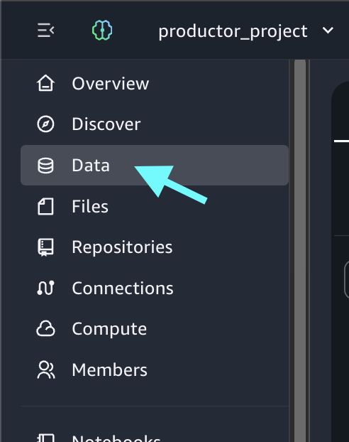
With conditional access in place, you can decide, based on your organization’s needs, whether access should be limited to trusted users on trusted networks, trusted devices, or both. This approach can help provide a more secure and compliant login experience that aligns SMUS access with your company’s broader identity and security strategy.


About the authors

Amit Samal

Amit Samal

Amit is a Sr. Delivery Consultant in World Wide Public Sector, Professional Services at AWS working with UKGI Customers. Amit has been with AWS for about 4 years and has been helping customers across the UKGI to design & implement secure, resilient and cost-effective workloads on AWS. Amit is passionate about all areas of technology, but has focus areas in Networking, Migrations, and Application Modernizations.

Manos Samatas

Manos Samatas

Manos is a Principal Solutions Architect in Data and AI with Amazon Web Services. He works with government, non-profit, education and healthcare customers in the UK on data and AI projects, helping build solutions using AWS. Manos lives and works in London. In his spare time, he enjoys reading, watching sports, playing video games and socialising with friends.

Scaling fine-grained access control for enterprise lakehouse using SageMaker Unified Studio and AWS Lake Formation

Post Syndicated from Chintan Agrawal original https://aws.amazon.com/blogs/big-data/scaling-fine-grained-access-control-for-enterprise-lakehouse-using-sagemaker-unified-studio-and-aws-lake-formation/

As enterprise lakehouses grow to thousands of tables across multiple business domains and regions, scaling fine-grained access control becomes a critical governance challenge. Data governance teams spend significant time manually granting table-level permissions, only to face permission drift, inconsistent enforcement, and limited auditability. Without a scalable approach, each new dataset requires manual policy updates, increasing the risk of unauthorized access and slowing time-to-insight for analysts and data scientists.

In this post, we show you how to solve this problem by combining AWS IAM Identity Center, AWS Lake Formation tag-based access control (TBAC), and trusted identity propagation in Amazon SageMaker Unified Studio. You deploy a complete governance architecture using AWS Cloud Development Kit (AWS CDK) that classifies data with LF-Tags, maps IAM Identity Center groups to tag-based policies, and enforces permissions at query time across analytics engines. The solution uses Apache Iceberg tables stored in Amazon Simple Storage Service (Amazon S3) and registered in the AWS Glue Data Catalog.

The core governance challenge

As organizations mature their lakehouse environments, governance complexity increases with each new dataset. Several challenges commonly emerge:

  • Explosive dataset growth: Iceberg-based lakehouses often contain thousands of tables distributed across raw, curated, and conformed zones. Each new dataset introduces additional governance requirements, making table-level permission grants operationally expensive.
  • Multi-domain data ownership: Enterprise lakehouses typically serve multiple business domains such as commercial analytics, clinical research, and regulatory reporting. These domains require strict isolation while still supporting controlled data sharing.
  • Regional data sovereignty: Organizations operating globally must enforce geographic boundaries for sensitive datasets. EU clinical trial data might be restricted by GDPR regulations, whereas US commercial datasets follow different compliance frameworks.
  • Sensitivity-based access controls: Within each domain, datasets vary in sensitivity. Pricing strategies, drug discovery research, and patient-related datasets require stricter access controls than standard operational data.
  • Role explosion: Pure RBAC approaches attempt to encode these dimensions into roles, leading to role proliferation. Manual Lake Formation grants at the table level create permission drift and limited scalability.

To address these challenges, enterprise lakehouse governance must satisfy several criteria:

  • Least-privilege access.
  • Dynamic scalability as new datasets are onboarded.
  • Multi-dimensional enforcement across domain, region, and sensitivity.
  • Auditability traceable to individual users.
  • Automation-ready, configuration-driven workflows.

TBAC addresses each of these challenges directly. Instead of granting permissions on individual tables, you define tag-based policies that automatically apply to any resource matching the tag expression. New datasets inherit access rules through tag inheritance, eliminating manual policy updates (solving explosive dataset growth). Domain and region tags enforce strict isolation between business units (solving multi-domain ownership and regional sovereignty). Sensitivity tags control access within domains without role proliferation (solving sensitivity-based controls and role explosion). The following sections describe the architecture that implements this model and walk you through deploying it end to end.

Reference architecture overview

The governance model integrates identity, metadata, and lakehouse services into a unified access architecture that enforces fine-grained permissions consistently across analytics and machine learning (ML) workloads. The architecture consists of five layers, each handling a distinct responsibility in the access control flow.

The following diagram illustrates the end-to-end architecture, showing how user identity flows from IAM Identity Center through SageMaker Unified Studio to Lake Formation for tag-based policy evaluation against the AWS Glue Data Catalog and Amazon S3 storage layer.

Architecture linking IAM Identity Center, SageMaker Unified Studio, Lake Formation, the Glue Data Catalog, and Amazon S3

Figure 1: End-to-end governance architecture for the enterprise lakehouse

1. Identity and authentication layer: IAM Identity Center manages user identities and group memberships, integrates with corporate identity providers, and provides centralized lifecycle management for enterprise users. IAM Identity Center groups represent business roles and serve as the principals that receive Lake Formation permissions.

2. Unified analytics and ML access layer: Amazon SageMaker Unified Studio serves as the primary interface where analysts, data scientists, and ML engineers discover datasets, run queries, and build ML workflows. Because SageMaker Unified Studio integrates with multiple compute engines, including Amazon Athena, AWS Glue, Amazon EMR, and Amazon Redshift, users can access data using their preferred analytics tools while maintaining consistent governance.

3. Governance and authorization layer: AWS Lake Formation provides fine-grained access control across AWS Glue catalog resources using LF-Tags. Instead of granting permissions directly on databases and tables, Lake Formation evaluates LF-Tag policies dynamically and grants or denies access at query time. Governance teams define access rules once, and Lake Formation automatically applies them to new datasets as they are onboarded.

4. Governance automation layer: Two AWS Lambda functions automate tag assignment and permission provisioning. JSON metadata configuration files drive both pipelines, so governance teams manage access control through configuration rather than manual console operations.

5. Metadata and storage layer: Apache Iceberg tables stored in Amazon S3 form the foundation of the lakehouse. You register these tables in the AWS Glue Data Catalog, which provides centralized metadata management and interoperability across analytics services. Lake Formation evaluates governance decisions at the catalog level rather than independently by each analytics engine.

End-to-end access flow

When a user queries a dataset from SageMaker Unified Studio, the following sequence occurs:

  1. The user authenticates through IAM Identity Center and accesses SageMaker Unified Studio.
  2. SageMaker passes the user’s identity context to downstream analytics services using trusted identity propagation.
  3. The analytics engine requests data access from Lake Formation.
  4. Lake Formation evaluates LF-Tag policies against the user’s IAM Identity Center group membership.
  5. Access is granted or denied dynamically at query time.

Because authorization decisions are centralized in Lake Formation, governance remains consistent regardless of which analytics engine the user employs.

Hybrid RBAC + ABAC governance model

The governance model combines identity context from IAM Identity Center with metadata-driven classification using LF-Tags. The following table summarizes how each layer contributes to the overall governance workflow.

Governance capability IAM Identity Center contribution Lake Formation LF-Tag contribution Governance outcome
Identity context Organizes users into groups aligned with business roles Evaluates permissions using group membership Role-aligned access boundaries
Data classification Provides role eligibility for data access Classifies datasets by domain, region, sensitivity, and layer Attribute-aware authorization
Scalability Simplifies user lifecycle management Automatically applies policies to newly tagged datasets Governance that scales with dataset growth
Operational model Centralizes role lifecycle operations Enables metadata-driven policy automation Reduced administrative overhead

IAM Identity Center defines who can request access, LF-Tags define what datasets are eligible, and Lake Formation enforces policies dynamically at query time.

Enterprise LF-Tag data model

A structured tagging strategy is the foundation of scalable Lake Formation governance. In this solution, the solution classifies datasets across four governance dimensions.

Tag Key Tag Values Purpose Example Usage
region us, eu, global Geographic data location Enforce GDPR compliance for EU data
domain commercial, clinical_research, regulatory Business domain Separate commercial from clinical data
data_class standard, sensitive, regulated Data sensitivity level Restrict access to sensitive pricing data
layer raw, curated, conformed Data processing stage Grant analysts access to curated data only

Together, these dimensions enable multi-dimensional authorization policies that reflect both organizational structure and regulatory requirements.

Tag inheritance and evaluation

LF-Tags can be applied at three resource levels within the Glue Data Catalog: database, table, and column. In this implementation, database-level tags define broad governance attributes (domain, region, layer), table-level tags capture dataset-specific sensitivity (data_class), and column-level tags can further restrict access to individual fields. Lake Formation evaluates the effective tag set at query time by combining inherited and explicitly assigned tags.

For example, a database tagged domain=commercial, region=us, layer=raw automatically applies those tags to all tables within it. A table-level data_class=sensitive tag supplements the inherited tags to distinguish sensitive pricing data from standard sales data. This inheritance model means new tables automatically receive governance coverage without manual tag assignment. To learn more, refer to Lake Formation tag-based access control best practices.

Prerequisites

Before deploying the solution, complete the following setup in the us-east-1 Region. Use the same AWS Region throughout all steps.

  1. AWS account and IAM Identity Center: Enable IAM Identity Center and create test users. Note your Identity Store ID from the IAM Identity Center console under Settings. For setup guidance, see Getting started with IAM Identity Center.
  2. Lake Formation configuration: Complete the following setup in the Lake Formation console:2.1. Change Data Catalog default permissions. In the navigation pane under Administration, choose Data Catalog settings. Uncheck Use only IAM access control for new databases and uncheck Use only IAM access control for new tables in new databases. Choose Save. This makes sure Lake Formation permissions govern access to databases and tables created by the CDK stacks.
    Lake Formation Data Catalog settings with both IAM-only access control checkboxes cleared

    Figure 2: Lake Formation Data Catalog settings with both IAM-only access control checkboxes unchecked

    2.2. Integrate with IAM Identity Center. Complete the prerequisites for IAM Identity Center integration with Lake Formation, including enabling trusted identity propagation.You don’t need to manually create a Lake Formation administrator. The CDK deployment in Step 2: Deploy all stacks automatically registers the required administrators via the LfAdminStack (see lf-admin-stack.ts). S3 data location registration is a post-deployment console step covered after the CDK creates the buckets.

  3. SageMaker Unified Studio: Create a SageMaker Unified Studio domain, select your IAM Identity Center instance for authentication, and enable trusted identity propagation. For a detailed walkthrough, see Accelerate your analytics with Amazon S3 Tables and Amazon SageMaker Lakehouse and enable trusted identity propagation for the domain.
  4. Local tooling: Install AWS Command Line Interface (AWS CLI), Python 3.x, Node.js 18+, AWS CDK CLI (npm install -g aws-cdk), and Git.

Solution overview

Now that you understand the governance model and tag taxonomy, the following section walks you through deploying the complete infrastructure and configuring access control.

The deployment uses AWS CDK (TypeScript) and consists of seven stacks that create the complete governance infrastructure. The CDK app manages stack dependencies automatically, so a single cdk deploy --all command deploys everything in the correct order.

The architecture uses a two-layer data lake pattern. The raw layer stores data as CSV files in Amazon S3, registered as external tables in the AWS Glue Data Catalog. The curated layer uses Apache Iceberg v2 tables for ACID transactions and schema evolution. Three business domains (US Commercial, EU Clinical Research, and Global Regulatory) each have one representative table per layer, giving six tables total.

Lake Formation tag-based access control (TBAC) governs all access using four tag dimensions:

Tag Key Values Purpose
domain commercial, clinical_research, regulatory Business domain isolation
region us, eu Geographic data boundary
data_class standard, sensitive, regulated Sensitivity classification
layer raw, curated Data layer identification

Step 1: Clone the repository and install dependencies

Clone the accompanying repository and install the CDK project dependencies:

git clone https://github.com/aws-samples/sample-aws-smus-governance-automation
cd aws-smus-governance-automation/cdk
npm install

The CDK project is written in TypeScript and uses aws-cdk-lib v2. The lib/ directory contains seven stack definitions, and bin/app.ts wires them together with explicit dependency ordering.

If this is your first CDK deployment in this account and Region, bootstrap the CDK environment. Bootstrapping provisions an S3 bucket and IAM roles that CDK uses to deploy assets:

cdk bootstrap aws://<ACCOUNT_ID>/us-east-1

Step 2: Deploy all stacks

Deploy the entire infrastructure with a single command. Pass your IAM Identity Center Identity Store ID as a CDK context variable:

cdk deploy --all -c identityStoreId=d-xxxxxxxxxx --require-approval never --region us-east-1

CDK will prompt for IAM permission changes on each stack. The --require-approval never flag auto-approves these so the deployment runs unattended.

CDK deploys the seven stacks in dependency order:

  1. LfSetupStack: Lake Formation admin registration + LF-Tags (domain, region, data_class, layer)
  2. GlueRawTablesStack: S3 bucket + three Glue databases + three CSV-backed tables.
  3. GlueCuratedTablesStack: S3 bucket + three Glue databases + three Iceberg v2 tables.
  4. SsoGroupsStack: three IAM Identity Center groups (DataLake-US-Commercial, DataLake-EU-Clinical-Research-Sensitive, DataLake-Regulatory)The three groups map to specific tag combinations that control data access:
    • DataLake-US-Commercial: domain=commercial, region=us, data_class=standard.
    • DataLake-EU-Clinical-Research-Sensitive: domain=clinical_research, region=eu, data_class=sensitive,regulated.
    • DataLake-Regulatory: domain=regulatory (all regions, all data classes within regulatory).

    The following table summarizes the user personas, their group assignments, and the data access each group provides:

  5. AssetTaggingAutomationStack: Tag automation Lambda.
  6. SsoPermissionAutomationStack: Permission automation Lambda.
  7. LfAdminStack: Registers CDK + Lambda roles as Lake Formation admins.

After deployment completes, review the CloudFormation stack outputs. They include S3 bucket names, database names, SSO group IDs, and Lambda function ARNs.

The following figure shows all seven CDK stacks deployed successfully in the CloudFormation console.

CloudFormation console showing all seven CDK stacks in CREATE_COMPLETE status

Figure 3: CloudFormation console showing all seven CDK stacks in CREATE_COMPLETE status

Register S3 data locations with Lake Formation: Now that the S3 buckets exist, register them with Lake Formation. In the Lake Formation console, under Administration, choose Data lake locations, then choose Register location. Register both buckets from the stack outputs (for example, s3://datalake-raw-data-<ACCOUNT_ID>-us-east-1 and s3://datalake-curated-data-<ACCOUNT_ID>-us-east-1). For IAM role, use the default AWSServiceRoleForLakeFormationDataAccess and choose Lake Formation as the permission mode. See Registering an Amazon S3 location for step-by-step instructions.

The following figure shows both data lake S3 locations registered in the Lake Formation console.

Lake Formation Data lake locations page listing the registered raw and curated S3 buckets

Figure 4: Lake Formation Data lake locations page with raw and curated S3 buckets registered

Step 3: Populate sample datasets

The scripts use Amazon Athena to insert sample data. Athena stores query results under the athena-results/ prefix in the shared governance metadata bucket (lf-governance-metadata-<ACCOUNT_ID>-<REGION>) created by the CDK deployment.

Populate the raw and curated tables:

cd ../scripts
python3 populate_raw_layer.py
python3 populate_curated_layer.py

Each script executes INSERT INTO statements through the Athena StartQueryExecution API and waits for completion. You should see success messages for all six tables (three raw, three curated).

After populating the tables, you can verify the data in the Glue Data Catalog. The following figure shows the six tables across the three raw and three curated databases.

AWS Glue Data Catalog showing the six databases and tables created by the deployment

Figure 5: AWS Glue Data Catalog showing the six databases and tables created by the CDK deployment

You can also preview the data by querying a table. The following figure shows sample data from the us_sales_summary table.

Athena query results showing sample commercial rows from the us_sales_summary table

Figure 6: Query results for the us_sales_summary table with sample commercial data

Step 4: Apply LF-Tags to data assets

The following diagram illustrates the governance automation flow, showing how metadata JSON configuration files drive the two Lambda pipelines for asset tagging and SSO permission management.

Governance automation flow with the asset tagging and SSO permission Lambda pipelines

Figure 7: Governance automation flow showing the asset tagging and SSO permission Lambda pipelines

The diagram shows two parallel pipelines, each following three steps:

Asset tagging pipeline (left):

  1. Metadata upload – A data governance administrator uploads metadata JSON files (metadata-raw-tables.json and metadata-curated-tables.json) to the asset-tagging/ prefix in the shared S3 governance metadata bucket. These files define which LF-Tags to assign to each AWS Glue database and table.
  2. Lambda processing – The S3 upload triggers the LakeFormationTagAutomation Lambda function, which reads the metadata and calls the Lake Formation API.
  3. Tag operations – The Lambda creates or updates LF-Tags, then assigns them to the target databases and tables in the AWS Glue Data Catalog.

SSO permission pipeline (right):

  1. Permission upload – Three permission JSON files (one per IAM Identity Center group) are uploaded to the sso-permissions/ prefix. These files define the LF-Tag policy expressions that control data access.
  2. Lambda processing – The upload triggers the LakeFormationSSOPermissionAutomation Lambda function.
  3. Permission operations – The Lambda grants tag-based permissions to the corresponding IAM Identity Center groups through the Lake Formation API.

Both pipelines log execution details to Amazon CloudWatch for monitoring and troubleshooting.

Two metadata JSON configuration files drive the asset tagging Lambda that declaratively define which LF-Tags to apply to each AWS Glue resource:

  • metadata-raw-tables.json: Tag definitions for the three raw layer databases and tables.
  • metadata-curated-tables.json: Tag definitions for the three curated layer databases and tables.

Each entry in these files specifies the following fields:

Field Description Example
catalog_id Your AWS account ID (Glue Data Catalog ID) 123456789012
resource_type DATABASE or TABLE DATABASE
database_name AWS Glue database name raw_us_commercial_db
table_name AWS Glue table name (only for TABLE entries) us_sales_summary
lf_tags Array of LF-Tag key/value pairs to assign [{“TagKey”:“domain”,“TagValues”:[“commercial”]}]
access_type Action to perform (GRANT) GRANT

Parameters you must update before invoking: Replace the catalog_id value in every entry of both files with your own AWS account ID. The database and table names match the resources created by the CDK stacks, so those should not be changed unless you customized the stack parameters.

The following snippet from metadata-raw-tables.json shows a database-level entry and a table-level entry:

[
  {
    "comment": "DATABASE LEVEL TAGS - US Commercial RAW Domain",
    "access_type": "GRANT",
    "resource_type": "DATABASE",
    "catalog_id": "<YOUR_ACCOUNT_ID>",
    "database_name": "raw_us_commercial_db",
    "lf_tags": [
      { "TagKey": "region", "TagValues": ["us"] },
      { "TagKey": "domain", "TagValues": ["commercial"] },
      { "TagKey": "layer", "TagValues": ["raw"] }
    ]
  },
  {
    "comment": "TABLE LEVEL TAGS - US Commercial RAW Table (Standard Access)",
    "access_type": "GRANT",
    "resource_type": "TABLE",
    "catalog_id": "<YOUR_ACCOUNT_ID>",
    "database_name": "raw_us_commercial_db",
    "table_name": "us_sales_summary",
    "lf_tags": [
      { "TagKey": "data_class", "TagValues": ["standard"] }
    ]
  }
]

The Lambda applies tags at two levels: database-level entries assign domain, region, and layer tags, while table-level entries assign the data_class tag (standard, sensitive, or regulated). Because of two-level tagging, new tables added to a tagged database automatically inherit the database-level tags. Only the table-specific data_class tag needs explicit assignment. To learn more about this pattern, refer to Lake Formation tag-based access control best practices.

Invoke the Lambda for both layers:

cd ../lf-asset-tagging-automation
aws lambda invoke \
    --function-name LakeFormationTagAutomation \
    --payload fileb://metadata-raw-tables.json \
    --cli-binary-format raw-in-base64-out \
    response.json

aws lambda invoke \
    --function-name LakeFormationTagAutomation \
    --payload fileb://metadata-curated-tables.json \
    --cli-binary-format raw-in-base64-out \
    response.json

Verify tag assignment using the GetResourceLFTags API:

aws lakeformation get-resource-lf-tags \
    --resource '{"Table":{"DatabaseName":"raw_us_commercial_db","Name":"us_sales_summary"}}' \
    --region us-east-1

You should see domain=commercial, region=us, layer=raw, and data_class=standard in the response.

The following figure shows the LF-Tags assigned to the us_sales_summary table in the Lake Formation console, confirming that both database-level inherited tags and table-level tags are applied correctly.

Lake Formation console showing inherited and table-level LF-Tags on the us_sales_summary table

Figure 8: LF-Tags on the us_sales_summary table showing inherited and table-level tags

Step 5: Provision SSO group permissions

Three permission JSON files (one per IAM Identity Center group) define the LF-Tag policy expressions. Update sso_group with the group UUID from the SsoGroupsStack outputs and identity_center_account_id with your AWS account ID. For detailed configuration, see the repository README.

[
  {
    "sso_name": "DataLake-US-Commercial",
    "sso_group": "<GROUP_UUID_FROM_CDK_OUTPUT>",
    "identity_center_account_id": "<YOUR_ACCOUNT_ID>",
    "resources": [
      {
        "resource_type": "DATABASE",
        "permissions": ["DESCRIBE"],
        "lf_tag_expression": [
          { "TagKey": "domain", "TagValues": ["commercial"] },
          { "TagKey": "region", "TagValues": ["us"] },
          { "TagKey": "layer", "TagValues": ["curated", "raw"] }
        ]
      },
      {
        "resource_type": "TABLE",
        "permissions": ["SELECT", "DESCRIBE"],
        "lf_tag_expression": [
          { "TagKey": "domain", "TagValues": ["commercial"] },
          { "TagKey": "region", "TagValues": ["us"] },
          { "TagKey": "data_class", "TagValues": ["standard"] },
          { "TagKey": "layer", "TagValues": ["curated", "raw"] }
        ]
      }
    ]
  }
]

Apply permissions for each group:

cd ../lf-sso-permission-automation
python3 lambda_function.py us-commercial-permissions.json
python3 lambda_function.py eu-clinical-research-sensitive-permissions.json
python3 lambda_function.py regulatory-permissions.json
aws lakeformation list-permissions \
    --principal '{"DataLakePrincipalIdentifier":"arn:aws:identitystore:::group/<GROUP_ID>"}' \
    --region us-east-1

Step 6: Validate fine-grained access control

With all permissions in place, validate that Lake Formation TBAC enforces the correct access boundaries by signing in to SageMaker Unified Studio as different IAM Identity Center users.

Test as Sarah (US Commercial Analyst) — Sarah belongs to DataLake-US-Commercial, which grants access to standard commercial data only.

SELECT * FROM raw_us_commercial_db.us_sales_summary LIMIT 10;

Sarah sees all rows and columns successfully:

SageMaker Unified Studio results: Sarah’s successful query on us_sales_summary

Figure 9: Sarah’s successful query on us_sales_summary in SageMaker Unified Studio

Querying outside her authorized domain returns an access denied error:

SELECT * FROM raw_eu_clinical_research_db.eu_drug_discovery LIMIT 10;
Access denied error when Sarah queries eu_drug_discovery outside her domain

Figure 10: Access denied when Sarah queries eu_drug_discovery, confirming TBAC enforcement

Test as Dr. Chen (EU Clinical Research Lead) — Dr. Chen can access sensitive and regulated EU clinical research data (eu_drug_discovery) but is denied access to US commercial data (us_sales_summary), confirming regional and domain isolation.

Query results showing Dr. Chen’s successful query on eu_drug_discovery

Figure 11: Dr. Chen’s successful query on eu_drug_discovery

Access denied error when Dr. Chen queries us_sales_summary

Figure 12: Access denied when Dr. Chen queries us_sales_summary

Test as Alex (Regulatory Affairs Specialist) — Alex’s tag expression uses only domain=regulatory without a region constraint, granting cross-regional access to regulatory data while maintaining strict isolation from commercial and clinical research domains.

Query results showing Alex’s successful query on fda_submissions

Figure 13: Alex’s successful query on fda_submissions

Access denied error when Alex queries us_sales_summary

Figure 14: Access denied when Alex queries us_sales_summary

These tests demonstrate that TBAC enforces fine-grained permissions based on user identity, data classification, regional boundaries, and domain separation, without per-table permission grants. As new tables are added and tagged, existing groups automatically gain or are denied access based on their tag expressions. This is the core advantage of TBAC over named resource permissions.

Audit user access with CloudTrail

A key benefit of integrating Lake Formation with IAM Identity Center is the detailed audit trail available through AWS CloudTrail. Filter Event history by Event name GetDataAccess to see every data access event. Each record includes the IAM Identity Center user UUID (userIdentity.onBehalfOf.userId), the specific table accessed (requestParameters.tableArn), and confirmation that trusted identity propagation was used (additionalEventData.LakeFormationTrustedCallerInvocation: true).

CloudTrail GetDataAccess event showing Identity Center user identity and table access details

Figure 15: CloudTrail GetDataAccess event showing Identity Center user identity and table access details

To resolve the user UUID to a human-readable name, query the Identity Store:

aws identitystore describe-user \
    --identity-store-id d-xxxxxxxxxx \
    --user-id <USER_UUID_FROM_EVENT> \
    --region us-east-1

This audit capability provides the detailed access logs required for HIPAA, GDPR, and FDA compliance, showing exactly which users accessed which data and when. Learn about configuring CloudTrail for Lake Formation in Logging Lake Formation API calls with CloudTrail.

Cleanup

Run cdk destroy --all to remove all stacks. Manually delete the retained S3 data buckets (datalake-raw-data-* and datalake-curated-data-*) and revoke any remaining Lake Formation permissions. For detailed cleanup steps, see the repository README.

Conclusion

In this post, we showed you how to implement scalable fine-grained access control for an enterprise lakehouse by combining AWS Lake Formation tag-based access control, IAM Identity Center, and trusted identity propagation in SageMaker Unified Studio. The four-dimension LF-Tag taxonomy, hybrid RBAC + ABAC governance model, and metadata-driven Lambda automation together create a governance architecture where new datasets automatically inherit access policies through tag inheritance, permissions scale without per-table grants, and every data access event is auditable to the individual user through CloudTrail.

To extend this solution, consider adding new business domains, implementing column-level security with LF-Tags, scaling to multi-account architectures with Lake Formation cross-account sharing, or integrating additional analytics services such as Amazon Redshift Spectrum or Amazon EMR.

Get started by deploying the CDK stacks from the accompanying repository. To learn more:


About the authors

Chintan Agrawal

Chintan Agrawal

Chintan is a Solutions Architect with over 7 years of experience, with a specialization in Analytics and Healthcare domain. He possesses a strong enthusiasm for assisting clients in discovering valuable insights from their data. Through his expertise, he constructs innovative solutions that empower businesses to arrive at informed, data-driven choices.

Chaitanya Vejendla

Chaitanya Vejendla

Chaitanya is a Senior Solutions Architect and part of Global Healthcare and Life Sciences industry division at AWS. He focuses on developing strategic plans for building an end-to-end analytical strategy for large biopharma, healthcare, and life sciences organizations. His expertise spans across data analytics, data governance, AI, ML, big data, and healthcare-related technologies.

Govern Amazon Redshift Data Warehouses Data Across Accounts using Amazon SageMaker Unified Studio

Post Syndicated from Bandana Das original https://aws.amazon.com/blogs/big-data/govern-amazon-redshift-data-across-accounts-with-sagemaker-unified-studio/

Managing data governance across multiple Amazon Redshift clusters in different AWS accounts presents significant challenges. Organizations operating multiple Amazon Redshift clusters across AWS accounts often rely on manual processes for secure data sharing, which increases operational overhead and governance requirements. In this post, we show you how to use Amazon SageMaker Unified Studio to implement cross-account data sharing in Amazon Redshift using data mesh principles. We demonstrate how to build a scalable data mesh architecture that supports secure, auditable data sharing across AWS accounts while reducing operational burden.

Amazon SageMaker Unified Studio as the backbone of our data mesh

Amazon SageMaker Unified Studio is a data and AI development service which brings together functionality and tools from existing AWS Analytics and AI and machine learning (ML) services, including Amazon EMR, AWS Glue, Amazon Athena, Amazon Redshift, Amazon Bedrock and Amazon SageMaker AI. With the service, organizations can catalog, discover, share, and govern data stored across Amazon Web Services (AWS) without relying on manual coordination between AWS accounts.

A data mesh is an architectural approach that treats data as a product, with decentralized ownership by data producers while maintaining centralized governance. This architecture separates source systems, data producers (data publishers), data consumers (data subscribers), and central governance. The solution we present is tailored for cross-AWS account usage, creating a foundation for data governance so you can share data across Amazon Redshift clusters in different AWS accounts.

Our proposed solution addresses the following common challenges that organizations face when sharing data across AWS accounts:

  • Manual, ad-hoc data sharing processes are replaced with automated, event-driven data publishing to the SageMaker Unified Studio catalog.
  • Inconsistent governance across different use cases is resolved through a consistent governance framework with proper access controls.
  • High load on producer Amazon Redshift clusters is reduced through decoupled publishing that lowers the operational burden on data producers.
  • Complex credential management is simplified using AWS Secrets Manager and AWS KMS encryption.
  • Lack of auditable data publishing is addressed with full traceability of access and permissions supported by the SageMaker Unified Studio service.

With this approach, you can help reduce the time and effort required for cross-account data sharing while maintaining security and governance standards.

Architectural overview

The architecture spans three AWS accounts, each with a distinct role in the data mesh:

Central Data Governance Account (Account A) hosts the Amazon SageMaker Unified Studio domain, which serves as the unified catalog and governance layer for data discovery, access control, and subscription management across accounts.

Data Producer (Account B) hosts the source of data and processing workflows. Raw data lands in an Amazon Simple Storage Service (Amazon S3) source bucket and is processed through AWS Glue extract, transform, and load (ETL) jobs or Amazon Redshift auto copy into the Amazon Redshift source database. Amazon Redshift credentials are securely stored in AWS Secrets Manager.

Data Consumer (Account C) hosts the target Amazon Redshift database and analytics workflows. After access is granted, consumers can query shared data and connect downstream visualization tools.

While this diagram shows a single producer and consumer for simplicity, in a real-world deployment there might be hundreds of producer and consumer accounts connecting through the central governance layer. Amazon SageMaker Unified Studio scales to support this by providing a single place for managing data products regardless of the number of participating accounts.

The data sharing workflow is driven by Amazon SageMaker Unified Studio. The data owner publishes data to the catalog, where it becomes discoverable by consumers across accounts. Consumers browse the catalog, subscribe to data products, and the data owner approves the request. After approval, Amazon SageMaker Unified Studio handles the cross-account sharing, granting the consumer access without requiring direct connectivity between producer and consumer Amazon Redshift clusters.

Publishing Amazon Redshift data assets to the data mesh

In a data mesh architecture, data producers need to make their data products discoverable and accessible across the organization. Amazon SageMaker Unified Studio provides a centralized catalog where data assets can be published for consumer subscription.

In practice, this means registering your data sources with the catalog so they can be discovered, governed, and subscribed to by consuming teams. This section walks through the steps required to register Amazon Redshift data sources with SageMaker Unified Studio.

Before you can publish data assets from your producer account, you need to complete several configuration steps across your Amazon Redshift cluster, AWS Secrets Manager, and Amazon SageMaker Unified Studio.

Prerequisites

  • Install the AWS Command Line Interface (AWS CLI) (v2.15+ recommended).
  • Obtain temporary credentials with permissions to administer each account (producer, consumer, and domain account)
  • IAM permissions required: redshift:* on the relevant clusters, secretsmanager:CreateSecret / PutResourcePolicy / TagResource, kms:CreateKey / PutKeyPolicy / TagResource, datazone:* for subscription-target creation, and iam:PassRole for the Amazon Redshift cluster role.
  • Amazon Redshift clusters must use RA3 node types (ra3.xlplus, ra3.4xlarge, or ra3.16xlarge). Data sharing is not supported on other node types.
  • Amazon SageMaker Unified Studio domain must already be created in Account A with the Tooling and LakeHouseCatalog blueprints available.
  • All resources must be in an AWS Region where Amazon SageMaker Unified Studio is available.

Step 1: Account association and blueprint enablement

To implement the data mesh architecture described in the previous section, you need to set up the following accounts and enable the required blueprints. This ensures that the central governance layer can discover and manage data assets across your producer and consumer accounts.

This post uses three separate AWS accounts to illustrate the cross-account data sharing pattern. However, Amazon SageMaker Unified Studio also supports publishing and subscribing to data within a single account or across any number of accounts depending on your organizational setup. Additionally, this walkthrough uses a provisioned Amazon Redshift cluster, but Amazon SageMaker Unified Studio also supports Amazon Redshift Serverless for both publishing and subscribing to data assets.

Step 2: Configure your Amazon Redshift cluster and credentials

  • In the producer account (Account B), the data to be shared resides in an Amazon Redshift cluster.
  • Verify that your Amazon Redshift cluster uses node types from the RA3 family.
  • Add the following tags to your Amazon Redshift cluster.

Amazon Redshift console showing tags added to the cluster

  • Create a superuser in Amazon Redshift for Amazon SageMaker Unified Studio. For the Amazon Redshift cluster, the database user you provide in AWS Secrets Manager must have superuser permissions. With superuser permission, your Amazon Redshift cluster can publish data and subscribe from the data mesh created with Amazon SageMaker Unified Studio, and it manages the subscriptions (access) on your behalf. For reference, see the note section in this QuickStart guide with sample Amazon Redshift data.

Tag key-value pairs configured on the Amazon Redshift cluster

  • Store the user’s credentials in Secrets Manager. Select the credential type, enter the credential values, and choose the AWS Key Management Service (AWS KMS) key with which to encrypt the secret

QuickStart guide note about providing superuser credentials for Amazon SageMaker Unified Studio

Tags on the AWS Secrets Manager secret including the Amazon Redshift cluster ARN

Resource policy added to the AWS Secrets Manager secret for Amazon SageMaker Unified Studio access

  • If your secret is encrypted with a customer managed AWS KMS key, append the key policy with the following statement and add a tag to the key: AmazonDataZoneEnvironment = All. You can skip this step if you’re using an AWS managed KMS key.
{
    "Sid": "AllowSMUSRolesSecretsAccess",
    "Effect": "Allow",
    "Principal": {
        "AWS": "*"
    },
    "Action": [
        "kms:Decrypt",
        "kms:DescribeKey",
        "kms:GenerateDataKey"
    ],
    "Resource": "*",
    "Condition": {
        "StringEquals": {
            "kms:ViaService": "secretsmanager.<<AWS_Region>>.amazonaws.com"
        },
        "StringLike": {
            "aws:PrincipalArn": [
                "arn:aws:iam::<<Data_Producer_Acct_Id(Account B)>>:role/aws-service-role/redshift.amazonaws.com/AWSServiceRoleForRedshift",
                "arn:aws:iam::<<Data_Producer_Acct_Id(Account B)>>:role/<<Redshift_Cluster_IAM_Role_Name>>",
                "arn:aws:iam::<<Data_Producer_Acct_Id(Account B)>>:role/datazone*",
                "arn:aws:iam::<<Data_Producer_Acct_Id(Account B)>>:role/service-role/AmazonSageMaker*"
            ]
        }
    }
},
{
    "Sid": "AllowSMUSRolesCreateGrant",
    "Effect": "Allow",
    "Principal": {
        "AWS": "*"
    },
    "Action": "kms:CreateGrant",
    "Resource": "*",
    "Condition": {
        "Bool": {
            "kms:GrantIsForAWSResource": "true"
        },
        "StringEquals": {
            "kms:ViaService": "secretsmanager.<<AWS_Region>>.amazonaws.com"
        },
        "StringLike": {
            "aws:PrincipalArn": [
                "arn:aws:iam::<<Data_Producer_Acct_Id(Account B)>>:role/aws-service-role/redshift.amazonaws.com/AWSServiceRoleForRedshift",
                "arn:aws:iam::<<Data_Producer_Acct_Id(Account B)>>:role/<<Redshift_Cluster_IAM_Role_Name>>"
            ]
        }
    }
}

Note: Enable automatic rotation. Configure Secrets Manager automatic rotation for this secret with a rotation interval appropriate to your security policy (for example, every 30 days). When implementing rotation, verify that the rotation Lambda function updates the credentials in both Secrets Manager and Amazon Redshift database users simultaneously. Note that Amazon SageMaker Unified Studio retrieves the secret at connection time, so rotation must produce credentials that are valid immediately upon storage: use the alternating-users rotation strategy if you need to avoid downtime during rotation. See the Secrets Manager rotation documentation for setup instructions.

Using Amazon Redshift Serverless?

  • Add the following Tags to the Amazon Redshift Serverless namespace and workgroup.

Tags added to the Amazon Redshift Serverless namespace and workgroup

  • In the Secrets Manager secret, verify the host points to your Serverless endpoint.

AWS Secrets Manager secret showing the host pointing to the Serverless endpoint

  • Add the following tags to the AWS Secrets Manager secret.

Tags added to the AWS Secrets Manager secret for the Redshift Serverless credentials

Publish Amazon Redshift data to the data mesh

With prerequisites complete, you can now register your Amazon Redshift cluster as a data source in Amazon SageMaker Unified Studio.

Step 1: Create an Amazon Redshift type connection

  • Sign in to Account B, navigate to your Amazon SageMaker Unified Studio associated domain, and open the Amazon SageMaker Unified Studio URL.

Amazon SageMaker Unified Studio associated domain sign-in page

Add an Amazon Redshift connection form in Amazon SageMaker Unified Studio

  • The newly created Amazon Redshift connection appears here.

Newly created Amazon Redshift connection listed in Amazon SageMaker Unified Studio

Step 2: Create the data source for your Amazon Redshift data warehouse

Add an Amazon Redshift data source form in Amazon SageMaker Unified Studio

Amazon Redshift data source configuration in Amazon SageMaker Unified Studio

  • For Publishing settings, choose whether assets are immediately discoverable in Amazon SageMaker Catalog.

Publishing settings controlling asset discoverability in the Amazon SageMaker catalog

Using Amazon Redshift Serverless?

When creating the connection and data source, use your workgroupName instead of clusterName. The rest of the data source configuration remains the same.

Step 3: Run the data source and publish the data asset to the data mesh

Data source run configuration in Amazon SageMaker Unified Studio

Data source run results in Amazon SageMaker Unified Studio

  • During creation of data source if you choose Publishing settings such as assets are immediately discoverable, the Amazon Redshift tables and views appear in the catalog as Published, ready for discovery and subscription by data consumers.

Published Amazon Redshift tables and views in the Amazon SageMaker catalog

Data discovery view in the Amazon SageMaker Unified Studio portal

Subscribe Amazon Redshift data through the data mesh

To complete the end-to-end test, you need to set up a consumer Amazon Redshift cluster in Account C.

Step 1: Setting up the consumer cluster

  • Follow the prerequisites from Steps 1 and 2 in the previous section, make sure the cluster and secret are properly tagged as in the following screenshots:
  • Amazon Redshift cluster tags:

Tags applied to the consumer Amazon Redshift cluster

  • Tags for the AWS Secrets Manager secret that stores the user credentials for the Amazon Redshift cluster:

Tags on the AWS Secrets Manager secret storing the consumer cluster credentials

Step 2: Connect the consumer cluster to the data mesh

  • Log into Amazon SageMaker Unified Studio and navigate to your consumer project.
  • In the Compute section of your project, choose Add compute, then choose Connect to existing compute resources.
  • Choose Amazon Redshift Provisioned.
  • Select your consumer Amazon Redshift cluster from the dropdown list and enter the Secrets Manager name.
  • Choose Add compute.
  • Your newly added Amazon Redshift cluster should now show as available.

Consumer Amazon Redshift cluster added as compute in Amazon SageMaker Unified Studio

  • The newly added Amazon Redshift cluster shows an Available state.

Consumer Amazon Redshift cluster showing an Available state

  • In the Data section you can see that objects (table/views) from Amazon Redshift cluster are visible and you can query them.

Data section showing Amazon Redshift tables and views available to query

Step 3: Creating a subscription target

  • Find the tooling environment ID: in your local terminal after obtaining correct credentials as a project member, run this command to find the tooling environment ID.
export REGION='<your-region>'
export SUBSCRIBER_PROJECT_ID='<your-project-id>'
export DOMAIN_ID='dzd-xxxxxxx'

aws datazone list-environments \
  --domain-identifier $DOMAIN_ID \
  --project-identifier $SUBSCRIBER_PROJECT_ID \
  --region $REGION
  • In the response, find and copy the tooling environment ID as shown in the following example.
{
    "items": [
        {
            "projectId": "<PROJECT_ID>",
            "id": "<ENVIRONMENT_ID>",
            "createdBy": "SYSTEM",
            "createdAt": "<TIMESTAMP>",
            "updatedAt": "<TIMESTAMP>",
            "name": "Tooling",
            "awsAccountId": "<AWS_ACCOUNT_ID>",
            "awsAccountRegion": "eu-west-1",
            "provider": "Amazon SageMaker",
            "status": "ACTIVE",
            "environmentConfigurationId": "<ENVIRONMENT_CONFIGURATION_ID>"
        }
    ]
}
  • Locate the Manage Access Role: In Account C, navigate to SageMaker Unified Studio and find the Tooling blueprint. In the Provisioning Tab you will find the Manage Access role and copy the value, as it is needed for the next CLI call.

Provisioning tab showing the Manage Access role for the Tooling blueprint

  • Create the Subscription Target.

With all the information collected, you can create the subscription target for the Amazon Redshift cluster as shown by the CLI call.

export TOOLING_ENV_ID='<tooling-environment-id>'
export AUTHORIZED_PRINCIPAL='datazone_env_<tooling-env-id>'
export MANAGE_ACCESS_ROLE='arn:aws:iam::<account-id>:role/service-role/AmazonSageMakerManageAccess-<domain-id>'

aws datazone create-subscription-target \
  --domain-identifier $DOMAIN_ID \
  --environment-identifier $TOOLING_ENV_ID \
  --name "RedshiftCluster-default-target" \
  --subscription-target-config '[{
    "formName": "RedshiftSubscriptionTargetConfigForm",
    "content": "{\"databaseName\":\"<db-name>\",\"secretManagerArn\":\"arn:aws:secretsmanager:<region>:<account>:secret:<secret-name>\",\"clusterIdentifier\":\"<cluster-id>\",\"schemaName\":\"<schema-name>"}"
  }]' \
  --applicable-asset-types RedshiftViewAssetType RedshiftTableAssetType \
  --manage-access-role $MANAGE_ACCESS_ROLE \
  --provider "Amazon SageMaker" \
  --type RedshiftSubscriptionTargetType \
  --authorized-principals $AUTHORIZED_PRINCIPAL

Using Amazon Redshift Serverless?

Use RedshiftServerlessSubscriptionTargetType as the --type and RedshiftServerlessSubscriptionTargetConfigForm as the formName in the subscription target config. Replace clusterIdentifier with workgroupName in the content JSON.

  • Verify the Subscription Target.

To verify that the subscription target was created successfully, make a last CLI call. You should find in the return a new subscription target with the name RedshiftCluster-default-target.

aws datazone list-subscription-targets \
  --environment-identifier $TOOLING_ENV_ID \
  --domain-identifier $DOMAIN_ID \
  --region $REGION

Step 4: Subscribing to data assets

  • Open the data catalog inside SageMaker Unified Studio and search for the assets you want to subscribe to.

Data catalog search for assets to subscribe to in Amazon SageMaker Unified Studio

Adding multiple databases and schemas

To publish assets from entirely different databases on the same Amazon Redshift cluster, you need to create a separate data source for each database, meaning repeating the steps mentioned in the section before. Each data source points to the same cluster connection but specifies a different database name. This approach gives you independent control over scheduling, publishing settings, and metadata generation for each database’s assets.

On the consumer side, each subscription target is bound to a specific database and schema combination. This is the target location where SageMaker Unified Studio will create views that give the consumer access to subscribed assets. To receive subscribed data in multiple databases or schemas, you create one subscription target per database-schema combination. For example, different teams within the consumer account might want the data materialized in their own schema. The following example shows this pattern:

# Subscription target for the sales schema
aws datazone create-subscription-target \
  --domain-identifier $DOMAIN_ID \
  --environment-identifier $TOOLING_ENV_ID \
  --name "RedshiftCluster-sales-target" \
  --subscription-target-config '[{ "formName": "RedshiftSubscriptionTargetConfigForm", "content": "{\"databaseName\":\"consumer_db\",\"secretManagerArn\":\"arn:aws:secretsmanager:<region>:<account>:secret:<secret-name>\",\"host\":\"<endpoint>\",\"port\":\"5439\",\"schemaName\":\"sales\"}" }]' \
  --applicable-asset-types RedshiftViewAssetType RedshiftTableAssetType \
  --manage-access-role $MANAGE_ACCESS_ROLE \
  --provider "Amazon SageMaker" \
  --type RedshiftSubscriptionTargetType \
  --authorized-principals $AUTHORIZED_PRINCIPAL

# Subscription target for the marketing schema
aws datazone create-subscription-target \
  --domain-identifier $DOMAIN_ID \
  --environment-identifier $TOOLING_ENV_ID \
  --name "RedshiftCluster-marketing-target" \
  --subscription-target-config '[{ "formName": "RedshiftSubscriptionTargetConfigForm", "content": "{\"databaseName\":\"consumer_db\",\"secretManagerArn\":\"arn:aws:secretsmanager:<region>:<account>:secret:<secret-name>\",\"host\":\"<endpoint>\",\"port\":\"5439\",\"schemaName\":\"marketing\"}" }]' \
  --applicable-asset-types RedshiftViewAssetType RedshiftTableAssetType \
  --manage-access-role $MANAGE_ACCESS_ROLE \
  --provider "Amazon SageMaker" \
  --type RedshiftSubscriptionTargetType \
  --authorized-principals $AUTHORIZED_PRINCIPAL

Verifying the audit trail

To substantiate the governance and traceability claims in this architecture, enable AWS CloudTrail in all three accounts with data events for Secrets Manager and KMS. Enable Amazon Redshift audit logging on clusters to capture connection and query activity through STL_CONNECTION_LOG and STL_QUERY. Subscription approvals and rejections are recorded by SageMaker Unified Studio and emitted to CloudTrail under the datazone.amazonaws.com event source. Look for CreateSubscriptionRequest, AcceptSubscriptionRequest, and RejectSubscriptionRequest events.

Clean up

If you deployed this solution for testing or evaluation purposes and no longer need the resources, we recommend cleaning up to avoid unnecessary costs. Amazon Redshift clusters, Secrets Manager secrets, and SageMaker Unified Studio projects all incur charges when left running. The following steps guide you through a structured teardown in the correct order: subscriptions first, then data assets, and finally the infrastructure itself. This order verifies that no orphaned resources remain.

  • Remove all subscriptions
  • Delete your data assets
  • Delete the projects
    • Delete the project within your SageMaker Unified Studio Domain after all subscriptions are removed. Make sure to delete both the consumer and producer projects.
  • Delete the SageMaker Unified Studio Domain in Account A.

Conclusion

In this post, we demonstrated how Amazon SageMaker Unified Studio simplifies cross-account data governance for Amazon Redshift. By implementing this solution, organizations can move away from ad-hoc, non-auditable data sharing processes to a secure, scalable, and fully governed approach. Amazon SageMaker Unified Studio serves as the central governance layer that data producers and consumers use to publish, discover, and subscribe to data products across AWS accounts. This turns a fragmented data landscape into a well-governed data mesh without the need for custom tooling or manual coordination.

With cross-account data sharing and governance in place, the natural next step is to use this well-governed data for machine learning and generative AI workloads. Because Amazon SageMaker Unified Studio brings together data, analytics, and AI capabilities in a single environment, teams can more efficiently transition from discovering and subscribing to data products to building ML models and generative AI applications, all within the same environment. This reduces the traditional friction between data engineering and data science, accelerating time to value. To get started with establishing your organization’s data mesh using Amazon SageMaker Unified Studio, follow the guidance for Setting up Amazon SageMaker Unified Studio.


About the authors

Bandana Das

Bandana Das is a senior Data Architect in Amazon Web Services and specializes in Data and Analytics. She builds event-driven data architectures to support customers in Data management and data-driven decision making. She is also passionate about enabling customers on their Data management journey to the cloud.

Sindi Cali

Sindi Cali is a ProServe Consultant with AWS Professional Services. She supports customers in building data driven applications in AWS.

Anirban Saha

Anirban Saha is a DevOps Architect at AWS, specializing in architecting and implementation of solutions for customer challenges. He is passionate about well-architected infrastructures, automation, data-driven solutions and helping make the customer’s cloud journey as smooth as possible.

Stoyan Stoyanov

Stoyan Stoyanov works for AWS as a DevOps Engineer. He has more than 10 years of experience in software engineering, cloud technologies, DevOps, data engineering, and security.

Viral Thakkar

Viral Thakkar is a Software Engineer at AWS, working on Amazon DataZone and Amazon SageMaker Unified Studio with a primary focus on distributed systems and data governance with deep expertise in building large-scale data analytics and pipelining solutions. He is passionate about tackling complex distributed systems challenges while also creating tools and automated scripts that simplify day-to-day workflows and improve productivity.

Introducing Apache Spark Connect support in AWS Glue interactive sessions

Post Syndicated from Zach Mitchell original https://aws.amazon.com/blogs/big-data/introducing-apache-spark-connect-support-in-aws-glue-interactive-sessions/

When we built AWS Glue interactive sessions, our goal was to make AWS Glue as interactive as running local Python from a notebook. We mostly succeeded. With a straightforward Python package and a Jupyter notebook, you could execute remotely against the AWS Glue ephemeral Spark backend. The Livy-based approach was ahead of its time, but it had limitations from its REST-based protocol. Running local PySpark unlocked powerful integrated development environment (IDE) features such as debugging and linting, so your environment could understand the code and help you develop Spark applications more quickly. Customers would often split their development work. They used local Spark (or Docker containers) to develop in an IDE on a small amount of data, then switched to AWS Glue interactive sessions to validate scaling and tuning against the full dataset.

With modern PySpark releases came a new protocol: Apache Spark Connect. Spark Connect bridges the gap between these two worlds: you develop in local Python, but execute on AWS Glue against actual data. Today, AWS Glue interactive sessions support Spark Connect natively. You can connect from any environment that supports the PySpark remote() API, including VS Code, PyCharm, Amazon SageMaker Unified Studio notebooks, and standalone Python applications. You don’t need to install specialized kernels or manage cluster infrastructure.

What Spark Connect changes

Spark Connect, introduced in Spark 3.4, decouples the Spark client from the server through a lightweight gRPC protocol. Instead of running your driver program on the cluster, your IDE communicates with a remote Spark server through a thin client layer. This architecture unlocks the key workflow improvement: you develop locally and execute remotely.

Spark Connect architecture diagram showing a thin client communicating with a remote Apache Spark server

Spark Connect architecture — thin client with the full power of Apache Spark

With Spark Connect support in AWS Glue interactive sessions, you get:

  • IDE freedom – Use VS Code, PyCharm, JupyterLab, or any Python environment. No kernel installation required.
  • Programmatic access – Build Spark into your Python applications and automation scripts with a standard SparkSession.builder.remote() call.
  • Serverless execution – AWS Glue provisions and manages the Spark cluster. You pay only for the data processing units (DPUs) consumed while your session is active.
  • Spark Connect monitoring – The Spark Live UI now includes a dedicated Connect tab showing active Spark Connect sessions and operations alongside the existing Jobs, Stages, and Executors views.

Getting started with SageMaker Unified Studio

Amazon SageMaker Unified Studio provides the most direct path to Spark Connect on AWS Glue. The notebook environment handles session creation, endpoint retrieval, and token refresh automatically, so no connection boilerplate is required.

Prerequisite: You need an Amazon SageMaker Unified Studio project to use this workflow. If you don’t have one, create a project in your SageMaker Unified Studio domain first.

To connect to an AWS Glue Spark Connect session:

  1. Sign in to SageMaker Unified Studio, choose your project, and create or open a Notebook.

A notebook open in SageMaker Unified Studio

A notebook open in SageMaker Unified Studio

  1. Choose the compute icon in the left toolbar to open the Compute environment panel. Expand the Spark section.

Compute environment panel in SageMaker Unified Studio with the Spark section expanded

The Compute environment panel with the Spark dropdown list

  1. Select a Glue Spark connection. Depending on your SageMaker domain configuration, you will see either default.spark or named connections such as project.spark.compatibility. Select the appropriate Glue (Spark) connection and choose Apply.

Notebook cell showing spark.version returns 3.5.6-amzn-1 after connecting to Glue Spark Connect

Connected to Glue Spark Connect — running spark.version returns ‘3.5.6-amzn-1’

After you make your selection, you’re connected. The spark session object is available natively. No imports or configuration are needed. Start running PySpark immediately:

spark.sql("SHOW DATABASES").show()

The session manages itself in the background, including automatic token refresh.

Using the sagemaker_studio SDK

The sagemaker-studio Python package extends the Spark Connect experience beyond SageMaker Unified Studio notebooks into local IDEs, continuous integration and continuous delivery (CI/CD) pipelines, and any Python environment. The sparkutils module handles session initialization and connection configuration in a single call. You get the same streamlined experience as in the notebook, anywhere you run Python:

from sagemaker_studio import sparkutils

# Initialize a Glue Spark Connect session using your project connection
spark = sparkutils.init(connection_name="default.spark")

# Run queries immediately
spark.sql("SHOW DATABASES").show()

You can also use sparkutils.get_spark_options() to retrieve pre-configured Java Database Connectivity (JDBC) options for reading and writing to data sources through your project connections. Supported sources include Amazon Redshift, Amazon Aurora, and Amazon DocumentDB (with MongoDB compatibility):

# Get connection options for a Redshift connection in your project
options = sparkutils.get_spark_options("my_redshift_connection")

# Read from Redshift via Spark Connect
df = spark.read.format("jdbc").options(**options).option("dbtable", "analytics.orders").load()
df.show()

Within SageMaker Unified Studio, the sagemaker-studio SDK is native to the environment. The spark session and sparkutils are available without installation. For local IDE use, install it with pip install sagemaker-studio and configure credentials through an AWS named profile or boto3 session.

How it works

Spark Connect sessions in AWS Glue use a three-step workflow:

  1. Create a session – Call the CreateSession API with SessionType set to SPARK_CONNECT. The session provisions in approximately 30 seconds.
  2. Retrieve the endpoint – Call GetSessionEndpoint to receive a sc:// gRPC endpoint URL and a time-limited authentication token.
  3. Connect with PySpark – Pass the endpoint and token to SparkSession.builder.remote() and start running Spark operations.

Spark Connect protocol flow from the DataFrame API to a logical plan, sent over gRPC and protobuf, with results streamed back over gRPC and Arrow

Spark Connect protocol flow — DataFrame API translated to logical plan, sent via gRPC/protobuf, results streamed back via gRPC/Arrow

Connecting with the low-level API

Some environments don’t have the sagemaker-studio SDK, such as custom containers, AWS Lambda functions, or non-Python toolchains. In these environments, or if you’re not using SageMaker Unified Studio, you can use the AWS SDK (Boto3) to manage sessions directly. The following example demonstrates the full workflow:

import time, boto3, urllib.parse
from pyspark.sql import SparkSession

glue = boto3.client("glue", region_name="us-east-1")

# 1. Create a Spark Connect session
session_id = "my-spark-connect-session"
glue.create_session(
    Id=session_id,
    Role="arn:aws:iam::123456789012:role/GlueServiceRole",
    Command={"Name": "glueetl"},
    GlueVersion="5.1",
    SessionType="SPARK_CONNECT",
    DefaultArguments={"--enable-spark-live-ui": "true"},
)

# 2. Wait for the session to reach READY
while True:
    status = glue.get_session(Id=session_id)["Session"]["Status"]
    if status == "READY":
        break
    time.sleep(5)

# 3. Get the Spark Connect endpoint
sc = glue.get_session_endpoint(SessionId=session_id)["SparkConnect"]
endpoint_url = sc["Url"]
auth_token = sc["AuthToken"]

# 4. Connect with PySpark
encoded_token = urllib.parse.quote(auth_token, safe="")
connection_string = f"{endpoint_url}:443/;use_ssl=true;x-aws-proxy-auth={encoded_token}"
spark = SparkSession.builder.remote(connection_string).getOrCreate()
spark.sql("SELECT 1 + 1 AS result").show()

Monitoring with Spark Live UI

When you enable the Spark Live UI at session creation, you gain access to a real-time dashboard showing:

  • Jobs and Stages – Track active, completed, and failed jobs with stage-level metrics.
  • Executors – Monitor memory usage, shuffle data, and executor health.
  • SQL – Inspect query plans and execution details.
  • Connect tab – View active Spark Connect sessions and operations (specific to Spark Connect).

Access the dashboard through the GetDashboardUrl API or directly from the AWS Glue console.

import boto3, webbrowser

glue = boto3.client("glue", region_name="us-east-1")
dashboard = glue.get_dashboard_url(
    ResourceId="my-spark-connect-session",
    ResourceType="SESSION",
)
webbrowser.open(dashboard["Url"])

In SageMaker Unified Studio, no API call is needed. Choose Ready in the notebook status bar to open the kernel info popover. From there, open the Spark UI link for the live dashboard or Spark Driver Logs for real-time log output.

Notebook status bar Ready button that opens the Spark UI and Spark Driver Logs links

Image showing “Ready” in the status bar to access Spark UI and Driver Logs directly from the notebook

Token refresh

Authentication tokens expire after 30 minutes. In SageMaker Unified Studio, this is handled automatically. For programmatic use, you can use a background thread to keep the connection alive. The following helper reconnects transparently before the token expires:

import threading, time, boto3, urllib.parse
from pyspark.sql import SparkSession

class GlueSparkConnect:
    """Maintains a SparkSession with automatic token refresh."""

    def __init__(self, session_id, region="us-east-1", refresh_margin=300):
        self.session_id = session_id
        self.glue = boto3.client("glue", region_name=region)
        self.refresh_margin = refresh_margin  # seconds before expiry to refresh
        self._lock = threading.Lock()
        self.spark = self._connect()
        self._start_refresh_loop()

    def _connect(self):
        sc = self.glue.get_session_endpoint(SessionId=self.session_id)["SparkConnect"]
        encoded_token = urllib.parse.quote(sc["AuthToken"], safe="")
        remote_url = f"{sc['Url']}:443/;use_ssl=true;x-aws-proxy-auth={encoded_token}"
        self._token_expiry = sc["AuthTokenExpirationTime"].timestamp()
        return SparkSession.builder.remote(remote_url).getOrCreate()

    def _start_refresh_loop(self):
        def _loop():
            while True:
                sleep_for = max(self._token_expiry - time.time() - self.refresh_margin, 30)
                time.sleep(sleep_for)
                with self._lock:
                    self.spark = self._connect()
        t = threading.Thread(target=_loop, daemon=True)
        t.start()

# Usage
session = GlueSparkConnect("my-spark-connect-session")
session.spark.sql("SELECT 1 + 1 AS result").show()

The background thread sleeps until 5 minutes before token expiry, then transparently reconnects. Because the daemon thread exits when your script ends, there is no cleanup required.

Getting started

To start using Spark Connect with AWS Glue interactive sessions:

  1. Use AWS Glue version 5.1 (Apache Spark 3.5.6).
  2. Install PySpark 3.5.6 locally: pip install pyspark==3.5.6.
  3. Grant your AWS Identity and Access Management (IAM) identity permissions for glue:CreateSession, glue:GetSession, and glue:GetSessionEndpoint.
  4. Create a session with --session-type SPARK_CONNECT and connect from your preferred environment.

VPC note: If you connect to AWS Glue interactive sessions through a virtual private cloud (VPC) endpoint, add the new Spark Connect endpoint (com.amazonaws.{region}.glue.sessions) to your VPC configuration. Existing AWS Glue VPC endpoints don’t cover Spark Connect traffic.

For detailed instructions, see Connecting to a Spark Connect session in the AWS Glue Developer Guide.


About the authors

Zach Mitchell

Zach Mitchell

Zach is a Senior Big Data Architect at AWS Worldwide Specialist Organization for Analytics. He works with customers to design and build data applications on AWS, with a focus on SageMaker Unified Studio, AWS Glue, and AWS Lake Formation. Outside of work, he enjoys building things with code and occasionally writing about it.

Shrey Malpani

Shrey Malpani

Shrey is a Senior Technical Product Manager at AWS Analytics. He is focused on building and scaling data processing, data integration, and data management capabilities across services like AWS Glue, Amazon EMR, and Amazon Redshift that help customers build AI-ready data platforms for their analytics or machine learning workflows.

Vaibhav Naik

Vaibhav Naik

Vaibhav is a Software Engineer at AWS Glue, where he leads the development of enterprise Generative AI managed services and Agentic data systems. He has over a decade of experience designing massive-scale cloud infrastructure and distributed computing platforms.

Tom Olson

Tom Olson

Tom is a Software Development Engineer on the AWS Glue team, focused on Interactive Sessions and operational excellence. He brings over 20 years of software development experience, including government contracting and EC2 Networking at AWS. Outside of work, he enjoys running and playing board games.

Gaurav Krishnan

Gaurav Krishnan

Gaurav is a Software Development Engineer at AWS Glue. He has a deep interest in distributed systems and creating low-friction developer experiences for interactive data workloads on Apache Spark. In his spare time, he enjoys running and trying new restaurants.

Modernizing financial analytics with Amazon SageMaker Unified Studio

Post Syndicated from Umang Aggarwal original https://aws.amazon.com/blogs/architecture/modernizing-financial-analytics-with-amazon-sagemaker-unified-studio/

Avanse Financial Services is one of India’s leading education loan providers. Their Data Engineering Team had built a data lake on AWS using Amazon Simple Storage Service (Amazon S3), Amazon Athena, and AWS Glue for data ingestion and processing. However, their analytics and reporting layer ran on an external analytics application that wasn’t integrated with AWS. Data had to be copied from Amazon S3 into this external application before analysts could run any report, its license consumed a significant portion of their budget despite low utilization, and every integration with AWS services required custom-built pipelines.

After evaluating their options, Avanse migrated to a cloud-native lakehouse architecture using Amazon SageMaker Unified Studio, which unified their data engineering, analytics, and artificial intelligence (AI) workflows in a single governed environment on AWS. In this post, we walk through their migration journey so you can adapt their approach to your own environment.

Why Avanse chose to modernize

The separation between their AWS data lake and their external analytics application created five problems:

  1. Daily data synchronization bottleneck. Every report required a 4-hour batch copy from Amazon S3 into the external analytics application before analysts could query it. Business decisions were based on data that was at least a day old.
  2. Fixed licensing costs disconnected from usage. The external analytics application charged an annual fee regardless of how many queries analysts ran. Avanse needed usage-based pricing that matched what they actually consumed, not a fixed fee for capacity they weren’t using.
  3. Limited auditability. The external analytics application ran on a shared server where different business units (risk, collections, portfolio management) shared the same resources. It lacked granular audit trails, making it difficult to trace who accessed what data and when, or to allocate costs per team.
  4. No centralized data discovery. Although AWS Glue Data Catalog managed schema metadata for the data lake, the external analytics application couldn’t access it. Analysts working in that application relied on folder structures and manual documentation to find the right datasets, slowing onboarding and increasing the risk of using outdated data.
  5. Disconnected from AWS services. The external analytics application couldn’t query data in Amazon S3 or use AWS Glue catalogs natively. Every data flow required connectors and custom-built pipelines, adding maintenance overhead.

Additionally, some datasets were stored on Network File System (NFS) storage outside of Amazon S3, creating another data silo that needed to be consolidated.

Avanse chose Amazon SageMaker Unified Studio because it addressed all five challenges: direct querying of data in Amazon S3 avoiding synchronization, usage-based compute through Amazon Athena and Amazon EMR Serverless, project-based isolation with per-project billing, lineage tracking with AWS IAM Identity Center, and native integration with their existing AWS services.

Solution overview

The core architectural change was moving from a two-application model to a single integrated stack:

Previous architecture
Avanse’s data ingestion and processing ran on AWS (Amazon S3, AWS Glue, Athena), but analytics and reporting ran on an external analytics application. Data had to be batch-copied from Amazon S3 into this external application daily before analysts could query it. Each system had its own access controls, and there was no shared catalog or lineage tracking between them.
New architecture
Analytics now run directly against data in Amazon S3 through Amazon SageMaker Unified Studio. There’s no data copy step. Analysts query the same data that the ingestion pipelines produce, using Athena for SQL and EMR Serverless for large-scale processing. Governance, access control, and lineage are centralized through IAM Identity Center and SageMaker Catalog.

The following diagram illustrates the target architecture. It follows a lakehouse pattern, storing data in open formats on Amazon S3 while maintaining ACID transaction support for the consistency financial regulators expect.

Three-layer lakehouse architecture for Avanse on AWS, showing the data layer with Amazon S3 and AWS Glue Data Catalog, the compute layer with Amazon SageMaker Unified Studio, AWS Glue ETL, AWS Lambda, Amazon EMR Serverless, Amazon SageMaker AI, and Amazon Bedrock, and the governance layer with AWS IAM Identity Center, SageMaker Catalog, and Amazon DataZone

The architecture has three layers:

  1. Data layer – Amazon S3 stores data in open formats (Parquet, Delta Lake) with S3 Intelligent-Tiering for automatic cost optimization. AWS Glue Data Catalog maintains schema metadata, making data discoverable across tools.
  2. Compute layer – Amazon SageMaker Unified Studio provides project-based workspaces organized by business function. Collections uses the built-in SQL Query Editor powered by Athena, Risk Reporting uses JupyterLab for interactive analysis, and MIS runs large-scale Spark jobs through Amazon EMR Serverless. AWS Glue ETL handles data transformations and AWS Lambda provides event-driven triggers for report generation. For machine learning (ML) workloads, Amazon SageMaker AI supports model training and deployment, with Amazon Bedrock available for generative AI capabilities such as enhancing risk narratives.
  3. Governance layer – IAM Identity Center provides SSO and audit logging across workspaces. SageMaker Catalog serves as the business glossary with data lineage tracking and access controls. Amazon DataZone connects components through a common metadata layer.

Migration journey

Avanse followed a five-phase approach. The timelines can be adapted to your environment, but the systematic progression from validation through production deployment is key.

Phase 1: Technical validation (72-hour workshop)

Avanse started with a focused 72-hour workshop using isolated SageMaker environments where developers could experiment without impacting production. Their team tested SQL analytics against existing Athena tables and validated that Python and PySpark could replicate their existing analytics workflows.

The team confirmed that querying data directly in Amazon S3 addressed their synchronization bottleneck entirely. The 4-hour daily data copy was no longer necessary, which validated the migration approach.

Phase 2: Data migration and storage optimization

Avanse migrated datasets from NFS storage and legacy analytics formats into Amazon S3, consolidating the data into a single location. They implemented S3 Intelligent-Tiering, which automatically moves data between access tiers based on usage patterns, optimizing costs without impacting retrieval performance.

They replaced legacy analytics connectors with native Athena workgroups within SageMaker Unified Studio, avoiding data synchronization entirely. Source data remained in Amazon S3, queryable by both Athena SQL and SageMaker notebooks, establishing a single source of truth.

Phase 3: Compute modernization

Avanse moved from a shared analytics server to project-based isolation in SageMaker Unified Studio. Each business function (Risk Reporting, Collections, MIS) received its own project with dedicated compute spaces running JupyterLab. Project-specific IAM execution roles provided access controls and cost allocation per business unit.

A single browser-based URL with multi-factor authentication (MFA) now provides access to SQL analytics using the built-in query editor, ML development in JupyterLab notebooks, and big data processing through Amazon EMR Serverless. This replaced the need for local analytics client installations.

Phase 4: Governance implementation

Avanse deployed SageMaker Catalog as their central business data catalog. Analysts now discover approved datasets through semantic search rather than navigating folder structures or relying on manual documentation. They mapped technical Athena table names to business terms. For example, analysts search for “collection efficiency” and find the relevant tables with descriptions, schemas, and lineage.

Lineage capture traces each metric in risk reports back to source tables, transformations, and intermediate datasets. Every action (notebook execution, SQL query, data access) is tied to IAM Identity Center users, creating the comprehensive audit trail their compliance team needed.

Phase 5: Use case migration

Rather than attempting a big-bang migration, Avanse moved critical workflows one at a time:

Portfolio MIS (Monthly/Fortnightly)
Previously required the daily 4-hour data copy from Amazon S3 into the external analytics application before report generation could begin. Avanse avoided the data synchronization step entirely and now generates MIS reports by querying existing Athena tables directly in Amazon S3. Because the source data was already on AWS, there was no need to involve the external application for this activity. Report generation dropped from hours to under 30 minutes.
Collection Efficiency and Bounce Calculation
Ported complex legacy analytics procedures for calculating metrics like collection efficiency and bounce rates to event-driven processing using AWS Glue ETL, AWS Lambda, and PySpark jobs for high-volume data aggregation. The serverless execution model charges only for compute time consumed.
EDW Risk Reporting
Large-scale regulatory joins of Enterprise Data Warehouse assets previously ran as legacy scheduled procedures. These now run as SQL queries in the SageMaker Unified Studio query editor, where analysts execute them on-demand or schedule them through Athena workgroups. The distributed query engine handles complex multi-table joins spanning millions of rows.
Scorecard Generation
Model building shifted from the external analytics application to SageMaker AI workflows. Data scientists use JupyterLab with Python libraries and deploy models directly to SageMaker endpoints, avoiding data movement between separate environments.

Overcoming technical challenges

One technical challenge was code migration. Avanse’s analytics code base contained years of accumulated proprietary scripts and procedures. Direct line-by-line translation was not practical. Instead, they took a pragmatic approach: basic data transformations moved to SQL in Athena, complex business logic was rewritten in PySpark for scalability, and statistical procedures were replaced with Python libraries like pandas and scikit-learn. The approach was to focus on what the code accomplishes, then implement it using cloud-native patterns.

The other technical challenge was performance validation. The team needed to confirm that querying data in Amazon S3 would deliver acceptable performance compared to the external analytics application’s in-memory processing. Queries against Parquet-formatted data in Amazon S3 using Athena delivered comparable performance for standard reporting workloads, while avoiding the 4-hour daily data synchronization step entirely. For large-scale regulatory joins spanning millions of rows, Amazon EMR Serverless provided distributed Spark processing that completed in minutes rather than the hours required in the external application.

Key outcomes

Area Result
Licensing costs Avoided external analytics application fees entirely
Storage costs Reduced through S3 Intelligent-Tiering, which automatically moves data between access tiers based on usage patterns
Report generation From over 4 hours (including data synchronization from Amazon S3 to the external analytics application) to under 30 minutes with direct Amazon S3 querying
Compliance audits From weeks of manual investigation to days with automated lineage reports
Compute costs Usage-based serverless model replaced always-on external analytics infrastructure
Collaboration Unified browser-based environment for data scientists, analysts, and engineers

“By adopting SageMaker Unified Studio, we as the Data Team eliminated legacy licensing costs, reduced storage and compute expenses with a serverless, usage-based model, and accelerated our periodic report generation. At the same time, we transformed compliance and collaboration by cutting audit timelines while unifying our teams in a single, efficient data environment.” – Komal Thakkar, AVP – Lead, Data Engineering, Avanse Financial Services

Best practices

Based on their experience, Avanse recommends:

  • Start with a workshop. Validate your specific use cases in a 72-hour technical validation before committing to full migration.
  • Migrate use cases, not code. Focus on what your analytics accomplish, then implement using cloud-native patterns rather than translating legacy scripts line by line.
  • Invest in governance early. Implement the data catalog and lineage tracking from day one.
  • Embrace project-based isolation. Organize around business functions for clear cost allocation and security boundaries.
  • Document business logic. Use migration as an opportunity to capture undocumented knowledge in the business glossary and dataset descriptions.

Conclusion

Avanse’s migration from an external analytics application to Amazon SageMaker Unified Studio consolidated their analytics stack into a single integrated environment on AWS. By querying data directly in Amazon S3 instead of copying it into the external application, they alleviated their biggest operational bottleneck. Project-based isolation replaced a shared server model, giving each business unit independent compute and clear cost visibility. And centralized governance through SageMaker Catalog and IAM Identity Center gave their compliance team the audit trails they had been missing.

The serverless, usage-based model means Avanse no longer pays for idle capacity. The lakehouse architecture supports new analytics patterns as they emerge, and native integration with AWS services, including generative AI through Amazon Bedrock, positions them to adopt new capabilities as their needs evolve.

Next steps

Start your analytics modernization journey by scheduling a 72-hour technical validation workshop. Contact your AWS account team to discuss your migration approach.

For more information, see:

Detecting fraud patterns across Snowflake and AWS using SageMaker Data Agent

Post Syndicated from Akash Gupta original https://aws.amazon.com/blogs/big-data/detecting-fraud-patterns-across-snowflake-and-aws-using-sagemaker-data-agent/

Financial services organizations increasingly run analytical workloads across multiple systems. For example, customers typically store transaction records in Snowflake for its concurrency handling during peak volumes, while they store risk scores, customer profiles, and behavioral signals on AWS. To bridge that divide, practitioners have had to stitch together manual exports, custom extract, transform, and load (ETL) code, and external business intelligence (BI) tools to query both sources, cache expensive aggregations, and visualize results.

Amazon SageMaker Data Agent now closes these gaps with three new capabilities in Amazon SageMaker Unified Studio notebooks: SQL analytics on Snowflake data sources, materialized view management, and interactive charting. Practitioners can use them together to query Snowflake alongside AWS data, pre-compute and schedule repeated aggregations, and create interactive visualizations from natural language prompts in a single notebook, without writing boilerplate code or switching tools.

In this post, we describe the challenges these capabilities address, introduce each one, and walk through a fraud analytics scenario that demonstrates them working together in an end-to-end investigation workflow.

Challenges with fraud detection

Fraud analytics teams working in SageMaker Unified Studio notebooks encounter several recurring friction points that slow their path from alert to insight:

  • Querying across AWS and third-party warehouses. Customers store transaction data in Snowflake and maintain risk scores and customer profiles on AWS. SageMaker Data Agent supported SQL generation for AWS-native engines: Amazon Athena, Amazon Redshift, Apache Spark, and DuckDB. However, it didn’t yet generate Snowflake-dialect SQL. This created a gap for customers working with data distributed across both AWS services and Snowflake. Analysts had to write Snowflake SQL manually and export results as CSV files to join with AWS data. The process consumed 1–2 hours before any actual investigation could begin.
  • Rich visualization requires coding expertise. When analysts want to plot query results, they must write Python code using packages like matplotlib, seaborn, or plotly. They must choose the right chart type, format axes, handle data transformations, and debug rendering issues. For fraud teams whose expertise is in investigation rather than data visualization code, each chart becomes a detour: either learn the package interface, ask an engineer for help, or export to an external BI tool. This slows the exploratory cycle that fraud investigations depend on, where every new angle (time-of-day patterns, category breakdowns, geographic clusters) ideally takes seconds, not minutes of code iteration.
  • Expensive repeated queries with no caching. Fraud signal queries flag transactions that exceed a customer’s historical average and compute risk-score distributions by merchant category. These queries re-scan entire tables on each execution. A team running the same aggregation every morning over millions of rows pays the full compute cost each time, with no mechanism to pre-compute results or schedule automatic refreshes. For fraud teams, this means investigations start with a 30-minute wait for queries that ran identically yesterday.

These three friction points (accessing data across platforms, visualizing it interactively, and operationalizing repeated analyses) are what the new Data Agent capabilities address together.

What’s new in Data Agent

Snowflake connectivity

SageMaker Data Agent can now connect to Snowflake data warehouses through connections registered in Amazon SageMaker Unified Studio. The agent discovers available Snowflake databases, browses schemas progressively (databases → schemas → tables → columns), and generates Snowflake-dialect SQL, including Snowflake-specific syntax like FLATTEN, VARIANT column access, and semi-structured data handling. Analysts query Snowflake tables alongside AWS data sources from a single notebook conversation, and the agent handles dialect differences automatically: Snowflake SQL for extraction, Spark SQL for Amazon Simple Storage Service (Amazon S3) Tables operations, with no manual translation required.

Materialized view management

Data Agent now creates and manages materialized views through natural language prompts. Analysts describe the aggregation they want, for example, “create a materialized view that flags transactions where risk_score is above 0.7, refreshed every 6 hours,” and the agent generates the Spark SQL DDL, including SCHEDULE REFRESH syntax. Materialized views store pre-computed results in Apache Iceberg format for fast repeated access, turning expensive full-table scans into sub-second queries. Supported operations include create, refresh, drop, describe, and scheduled refresh. When asked, Data Agent can also analyze notebook query patterns and recommend which queries would benefit from materialization.

Interactive charting

Instead of generating matplotlib code that produces static images, Data Agent now creates native interactive chart cells powered by Vega-Lite. Supported chart types include bar, line, scatter, pie, area, heatmap, and more. Charts render inline in the notebook with hover tooltips, zoom, and filtering. Analysts can reconfigure them through the sidebar or by typing inline instructions like “change this to a heatmap showing volume by hour and category.” This removes the cycle of modifying Python plotting code or exporting to an external BI tool every time the analysis needs a different view.

Detecting fraud patterns across Snowflake and AWS: a walkthrough

Solution overview

In this section, we walk through how these three capabilities work together in a realistic fraud investigation. A fraud analytics lead at a mid-size fintech processes a high volume of card transactions daily. Customers store transaction data in Snowflake and maintain customer risk profiles on AWS.

This morning, the real-time alerting system flagged an unusual spike in declined transactions from a cluster of new accounts, all purchasing high-value electronics. The analyst suspects a fraud ring using synthetic identities, fabricated customer profiles that pass initial verification but share telltale patterns like similar device fingerprints or overlapping IP ranges. The analyst has three goals:

  • Confirm the fraud ring hypothesis. Determine whether the flagged accounts share device fingerprints, IP ranges, or behavioral patterns indicating coordinated fraud.
  • Quantify the exposure. Calculate total fraudulent transaction volume and identify all affected accounts, not only the ones that triggered today’s alert.
  • Set up ongoing monitoring. Create a reusable, auto-refreshing query so the team catches the next ring faster.

The analyst wants to do all of this without leaving the SageMaker notebook, without writing boilerplate data-engineering code, and within a single morning standup cycle so the investigations team can be briefed by noon.

How Data Agent approaches this analysis

Data Agent is context-aware. It discovers your actual table names, column schemas, and data source connections through Amazon SageMaker Unified Studio rather than requiring you to specify them manually. It generates SQL in the correct dialect for each source (Snowflake SQL for Snowflake, Spark SQL for S3 Tables) and operates within your existing AWS Identity and Access Management (IAM) permissions boundaries.

You interact with Data Agent in two modes: the Agent Panel for multi-step investigations like the example walkthrough that follows, where each prompt builds on previous context, and inline interactions for quick adjustments like “change this to a heatmap” directly on a chart cell.

Prerequisites

Before starting this walkthrough, verify that you have:

  • An Amazon SageMaker Unified Studio domain with a project configured.
  • A Snowflake account with a warehouse and USAGE grants on the database and schemas you want to query.
  • A Snowflake connection registered in your SageMaker Unified Studio project.
  • An S3 Tables catalog in your project containing customer data (or equivalent AWS-hosted tables for joining with Snowflake data).
  • A notebook open in SageMaker Unified Studio with Data Agent available in the chat panel.

Step 1: Explore Snowflake transaction data

What the analyst wants: Before investigating the fraud ring, the analyst must understand what data is available in Snowflake and verify recent transactions are accessible. The schema isn’t memorized (the payments team manages these tables), so Data Agent needs to discover the structure.

In the SageMaker notebook Agent Panel, the analyst types:

“Show me a preview of transactions over $500 for the last 24 hours. I’m looking for repeated high-value purchases that might indicate synthetic identity fraud.”

What Data Agent does for you: Data Agent discovers the Snowflake connection through SageMaker Unified Studio, browses the available databases, and locates PAYMENTS_DBCARD_TRANSACTIONS schema → transactions table. It surfaces the column structure (transaction_id, customer_id, amount, merchant_category, transaction_timestamp, device_fingerprint, ip_address) so the analyst can confirm the right data is available without writing a single DESCRIBE TABLE statement.

Data Agent then generates a Snowflake-dialect SQL query to preview the last 24 hours of high-value transactions (amount > $500), returning hundreds of results. The preview immediately reveals what was suspected: alongside legitimate high-value purchases (mortgage payments, business supplies), there are clusters of electronics purchases at similar price points from different customer_id values but the same device_fingerprint, a classic synthetic identity pattern.

Data Agent querying Snowflake transaction data and generating equivalent code in the cell

Figure 1: Data Agent querying Snowflake transaction data and generating equivalent code in the cell.

Notebook cell results showing high-value Snowflake transactions

Figure 2: Displaying results when the notebook cell runs.

Step 2: Land Snowflake data into S3 Tables and join with risk profiles

What the analyst wants: Pulling historical high-value transactions into S3 Tables makes this data available for downstream analysis, including the materialized view that will cross-reference risk profiles automatically.

“Load the last 90 days of transactions where amount is greater than 500 into S3 Tables.”

What Data Agent does for you: Data Agent queries Snowflake to extract a large volume of high-value transactions from the last 90 days, converts the result to a PySpark DataFrame, creates an Apache Iceberg table at payments.fraud_analytics.high_value_transactions, and writes all the rows. Data Agent stores the transaction data (transaction_id, customer_id, amount, merchant_category, transaction_timestamp, device_fingerprint, ip_address) as Iceberg in S3 Tables, allowing you to query it entirely on AWS.

Data Agent handles the cross-source complexity: Snowflake-dialect SQL for extraction, automatic schema inference for the Iceberg table, and PySpark for the write. The analyst didn’t write a single line of ETL code.

Prompt sent to Data Agent to land Snowflake transactions into an S3 Tables

Figure 3: Sending a prompt to land Snowflake transactions into an S3 Tables catalog.

Generated PySpark code that reads transaction data from Snowflake

Figure 4: Reading data from Snowflake using code Data Agent generated.

Generated cell creating an S3 Tables Iceberg table populated with Snowflake data

Figure 5: Data Agent creating a new cell to create an S3 Tables Iceberg table and populate it with the Snowflake data.

Step 3: Create a materialized view for ongoing fraud monitoring

What the analyst wants: The pattern is confirmed, but re-running this expensive join across two tables every morning isn’t sustainable. A pre-computed view that automatically refreshes and surfaces transactions from high-risk customers means tomorrow’s investigation starts with answers instead of queries (goal #3, ongoing monitoring).

“Create a materialized view called mv_fraud_signals that joins high_value_transactions with customer_risk_profiles, flagging transactions where risk_score is above 0.7. Refresh it every 6 hours.”

What Data Agent does for you: Data Agent browses the S3 Tables catalog to discover both tables and their schemas, generates the Spark SQL DDL with SCHEDULE REFRESH EVERY 6 HOURS, and creates an INNER JOIN on customer_id with a risk_score > 0.7 filter. The resulting materialized view contains only the high-risk subset of transactions, and subsequent queries against it return significantly faster compared to a full table scan.

Data Agent can also recommend materialized views when asked. If the analyst prompts “analyze my notebook and suggest which queries would benefit from materialized views,” Data Agent examines query patterns and suggests candidates. This is useful when a team runs the same expensive aggregations repeatedly without realizing a materialized view would help.

New cell created by Data Agent to create the mv_fraud_signals materialized view

Figure 6: Data Agent creates a new cell to create the materialized view.

Generated query against the newly created materialized view

Figure 7: Data Agent adds code to query the newly created materialized view.

Step 4: Visualize fraud patterns with interactive charting

What the analyst wants: The data is ready, but the investigations team needs a clear visual story by noon to see which merchant categories are targeted and what time of day the fraud occurs, so they can build detection rules. The team needs interactive charts that can be explored on the fly, not static matplotlib images that need regenerating every time someone asks “what about category X?”

“Show me a scatter plot of flagged transactions: amount vs risk_score, colored by merchant_category.”

What Data Agent does for you: Data Agent queries the materialized view, generates a Vega-Lite specification, and renders an interactive scatter plot directly in the notebook cell, with no matplotlib code and no BI tool export. Hovering over any point reveals the transaction details. A dense cluster immediately stands out: Electronics & Computers transactions with risk scores between 0.75–0.95, all in the $950–$1,000 range.

Generated scatter plot of flagged transactions colored by merchant category

Detail view of the scatter plot highlighting the Electronics cluster

Figures 8, 9, and 10: Data Agent creates a scatter plot showing a dense cluster of Electronics transactions in the $950–$1,000 range with risk scores between 0.75–.95.

The analyst follows up with a second prompt to explore temporal patterns:

“Change this to a heatmap showing transaction volume by hour of day and merchant category.”

What Data Agent does for you: Data Agent generates a new heatmap visualization from the same materialized view. The heatmap reveals that Business Supplies and Mortgage Payments maintain steady transaction volumes throughout the day. However, Electronics shows a distinctly uneven temporal distribution, with noticeable volume dips during early morning hours (midnight to 5 AM) and late evening. This variability, absent in legitimate purchase categories, is a signal the detection rules team can act on immediately.

Heatmap of transaction volume by hour and merchant category

Detail view of the heatmap showing off-hours dips in the Electronics row

Figures 11 and 12: Data Agent creates a heat map to show transaction volume by hour of day and merchant category, revealing uneven temporal distribution in high-risk categories.

From insight to action

This investigation, from Snowflake connection to visual evidence, streamlined a workflow that previously required significant time across multiple tools. The analyst shares the notebook link with the investigations team, who confirm a fraud ring of dozens of synthetic identities responsible for significant fraudulent purchases. The temporal pattern, uneven Electronics transaction distribution with off-hours variability, is added to the company’s real-time detection rules that same afternoon.

The materialized view continues refreshing every 6 hours. The next morning, it flags three new accounts matching the same pattern, caught within hours of their first transaction instead of days.

Why SageMaker Data Agent for fraud analytics

This walkthrough demonstrates three new capabilities working together:

  • SQL analytics on Snowflake data sources removed the CSV export and manual ETL that consumed half of the investigation time.
  • Materialized view management turned a one-time query into persistent, auto-refreshing monitoring, transforming reactive investigations into proactive detection.
  • Interactive charting kept the entire analysis in the notebook, removing the BI tool context switch and making the inline exploration that revealed the Electronics temporal anomaly possible.

For the team, the combined effect is a reduction in time-to-insight, allowing faster fraud pattern analysis. This means daily fraud pattern reviews instead of weekly, and an investigation workflow that’s reproducible. The notebook itself serves as documentation for compliance and audit purposes.

Cleanup

The walkthrough creates notebook cells, SQL queries, and materialized views in your SageMaker Unified Studio session. To remove the generated cells, delete them from your notebook or delete the notebook itself.

If you created resources specifically for this walkthrough, remove the following to avoid ongoing charges:

  • Materialized view. In the notebook Agent Panel, prompt: “Drop the materialized view mv_fraud_signals.” This removes the Iceberg table from S3 Tables and cancels the scheduled refresh. Alternatively, run the Spark SQL statement DROP MATERIALIZED VIEW payments.fraud_analytics.mv_fraud_signals directly.
  • Landed Iceberg tables. Drop any tables created during the data landing step (for example, payments.fraud_analytics.high_value_transactions) by prompting Data Agent or running DROP TABLE in a Spark SQL cell. This removes the data from S3 Tables and the underlying Amazon Simple Storage Service (Amazon S3) storage.
  • SageMaker Unified Studio domain. If you created a domain solely for this walkthrough, delete it to stop incurring charges. Refer to the SageMaker Unified Studio administration guide for deletion steps.
  • Amazon S3 storage. Verify that dropping the materialized view and Iceberg tables removed the associated S3 objects. If residual Iceberg metadata files remain in your S3 Tables bucket, delete them manually.
  • Snowflake compute. No persistent Snowflake resources are created. Queries use your existing warehouse. Review your Snowflake query history to estimate the compute credits consumed during the walkthrough.

Conclusion

In this post, we walked through three new capabilities in Amazon SageMaker Data Agent for notebooks: Snowflake connectivity, materialized views, and native interactive charting. Using a fraud analytics scenario, we demonstrated how these features work together. We connected to a Snowflake warehouse to explore transaction data, landed results into S3 Tables and joined them with AWS-hosted risk profiles, created a materialized view for ongoing fraud monitoring, and visualized patterns with interactive charts that revealed temporal anomalies in Electronics transactions linked to dozens of synthetic identities.

These capabilities are available now in Amazon SageMaker Unified Studio. To get started, open a notebook in your SageMaker Unified Studio domain and begin a conversation with Data Agent in the chat panel.

To learn more, see the following resources:


About the authors

Akash Gupta

Akash Gupta

Akash is a Software Development Engineer on the Amazon SageMaker Unified Studio team, where he builds integrated tools and agentic experiences. An alumnus of Santa Clara University, he is passionate about building scalable solutions that simplify how customers interact with their data. In his spare time, he enjoys singing and cooking.

Mukesh Sahay

Mukesh Sahay

Mukesh Sahay is a Software Development Engineer at Amazon SageMaker, focused on building the SageMaker Data Agent. The agent provides intelligent assistance for code generation, error diagnosis, and data analysis recommendations for data engineers, analysts, and scientists. His work spans agentic AI architectures that transform natural language prompts into executable code and analysis plans across diverse data sources. An alumnus of San Jose State University, Mukesh brings over a decade and a half of experience in building scalable, intelligent data systems.

Eason Ma

Eason Ma

Eason is a Software Development Engineer within SageMaker’s Agentic AI Experiences. His focus is on building agentic infrastructure and intelligent data experiences that help users seamlessly interact with their data across multiple sources. He holds a Master’s in Computer Science from the University of Illinois at Urbana-Champaign and a Bachelor’s in Computer Science from the University of Tennessee, Knoxville. A proud Vol, he brings that same volunteer energy to everything he builds.

Anagha Barve

Anagha Barve

Anagha is a Software Development Manager on the Amazon SageMaker Unified Studio team. Her team is focused on building tools and integrated experiences for the developers using Amazon SageMaker Unified Studio. In her spare time, she enjoys cooking, gardening and traveling.

Siddharth Gupta

Siddharth Gupta

Siddharth is heading Generative AI within SageMaker’s Unified Experiences. His focus is on driving agentic experiences, where AI systems act autonomously on behalf of users to accomplish complex tasks. An alumnus of the University of Illinois at Urbana-Champaign, he brings extensive experience from his roles at Yahoo, Glassdoor, and Twitch.

AI-assisted data development with Kiro and SageMaker Unified Studio

Post Syndicated from Zach Mitchell original https://aws.amazon.com/blogs/big-data/ai-assisted-data-development-with-kiro-and-sagemaker-unified-studio/

AI coding assistants are transforming software development, but data engineering presents unique challenges: governed data access, shared compute environments, and compliance controls that are designed to remain in place. How do you bring the power of agentic AI development into a governed data environment? With the AWS Toolkit for Visual Studio Code, you can connect Kiro, VS Code, or Cursor directly to Amazon SageMaker Unified Studio.

When you connect your editor to a SageMaker Unified Studio Space (a cloud-based compute environment inside your project), you get AI-assisted development with your preferred tools while your data governance, project permissions, and compute are managed by SageMaker Unified Studio. Additionally, SageMaker Unified Studio automatically generates steering files (like AGENTS.md) that provide your AI assistant with context about your project environment, so it understands your data and project configuration from the first prompt.

This post demonstrates the integration using Kiro. The same Remote Access connection works with VS Code and Cursor. The post starts by showing what you can do with this integration: using natural language to explore and analyze data in a governed environment. We then walk through the setup so you can try it yourself.

What’s new

With the AWS Toolkit, you can connect Kiro, VS Code, and Cursor to your SageMaker Space over a secure SSH tunnel. No additional extensions or SSH key management required. After the connection is established, your IDE has full access to your Space’s file system, compute, and data services.

Two capabilities make this especially powerful for data work:

  • Automatic AI steering – When connecting Kiro to SageMaker Unified Studio,  Kiro generates AGENTS.md and smus-context.md files that provide your AI assistant with context about your environment, including project configuration, environment details, and utilities for discovering your data catalog and project structure. Kiro detects these files automatically; other editors can use them as context for their own AI features.
  • MCP server support – have Kiro discover and configure itself for the Model Context Protocol servers on your remote SageMaker space ( like smus_local and aws-dataprocessing) to give your agent direct access to your AWS Glue Data Catalog, Amazon Athena queries, and SageMaker Unified Studio project metadata.

The following diagram shows how the components connect:

Architecture diagram: How the components connect

See it in action: AI-assisted development with governed data

Before walking through the setup, we explain what you can do with this integration. This walkthrough uses Kiro as the editor. With Kiro connected to a SageMaker Unified Studio Space, MCP servers configured, and steering documents in place, we can use natural language to explore data and build analytics. The AI assistant has all the context it needs to do this well.

Note: Agentic AI output is nondeterministic. The exact code, tool choices, and responses Kiro produces will vary between sessions, even with the same prompt. The following walkthrough shows one representative session. Your experience will differ in the specifics, but the patterns and capabilities demonstrated here are consistent.

Step 1: Explore the data

Start with a simple prompt:

show my databases and the tables I have access to

Even with native MCP tools available, Kiro often prefers the AWS Command Line Interface (AWS CLI) and bash to retrieve information. This is expected and typically does not affect the outcome. If you prefer MCP tools for every operation, you can add that preference to a steering document.

Kiro used the sagemaker_studio SDK to discover the catalog:

python3 -c "
from sagemaker_studio import Project
project = Project()
conn = project.connection()
catalog = conn.catalog()
print('Databases:')
for db in catalog.databases:
    print(f'  - {db.name}')
"
Databases:
  - default
  - sagemaker_sample_db

Then it drilled into the table schema:

python3 -c "
from sagemaker_studio import Project
project = Project()
conn = project.connection()
catalog = conn.catalog()
db = catalog.database('sagemaker_sample_db')
print('Tables in sagemaker_sample_db:')
for t in db.tables:
    print(f'  - {t.name}')
    print(f'    Columns: {[(c.name, c.type) for c in t.columns]}')
"
Tables in sagemaker_sample_db:
  - churn
    Columns: [('state', 'string'), ('account_length', 'int'),
              ('area_code', 'string'), ('phone', 'string'),
              ('intl_plan', 'string'), ('vmail_plan', 'string'),
              ('vmail_message', 'int'), ('day_mins', 'double'),
              ('day_calls', 'int'), ('day_charge', 'double'),
              ('eve_mins', 'double'), ('eve_calls', 'int'),
              ('eve_charge', 'double'), ('night_mins', 'double'),
              ('night_calls', 'int'), ('night_charge', 'double'),
              ('intl_mins', 'double'), ('intl_calls', 'int'),
              ('intl_charge', 'double'), ('custserv_calls', 'int'),
              ('churn', 'boolean')]

Kiro discovered the sagemaker_sample_db.churn dataset, a sample dataset that ships with SageMaker Unified Studio containing 10,000 rows and 21 columns of customer churn data (state, account length, call minutes, service calls, churn flag, and more). Notice that we did not write any of this code. We asked a question in natural language, and Kiro chose the right SDK calls, explored the catalog, and surfaced the results.

Another, more natural way to get the same answer is to ask directly. Prompting “Let us sample the churn table.” yields the same catalog paths and schema output, along with additional metrics like row count and a data sample, all from a single conversational prompt:

SageMaker Unified Studio console showing the sagemaker_sample_db.churn dataset listed in the catalog

Figure 1 — The sagemaker_sample_db.churn dataset in the catalog

Schema view showing the 21 columns of the churn table including state, account_length, call minutes, and the churn boolean

Figure 2 — Churn dataset schema with 21 columns

from sagemaker_studio import sqlutils
result = sqlutils.sql(
    'SELECT COUNT(*) AS total_rows FROM sagemaker_sample_db.churn',
    connection_name='default.sql'
)
print('=== Total Row Count ===')
print(result)
=== Total Row Count ===
   total_rows
0       10000

With the schema and row count in hand, Kiro sampled the data to round out its understanding of the dataset:

Comprehensive data sample showing 10 rows from the churn table with all 21 columns populated

Figure 3 — Comprehensive data sample after Kiro catalog exploration

Step 2: Run analytics with full context

With the data explored, ask Kiro to run a data quality evaluation:

Can we run basic statistical evaluations for data quality?

Because Kiro had already explored the catalog and sampled the data, it made smart choices about how to run the analysis. Instead of using PySpark for this 10,000-row table, Kiro used Athena using sqlutils to run the evaluation directly. It produced a thorough data quality report:

  • 10,000 rows, 21 columns, zero nulls across all columns. Clean on that front.
  • 5,000 duplicate rows (50 percent). Significant, worth investigating before modeling.
  • Outliers minimal. Most columns have less than 1 percent outlier rate by IQR.
  • Churn is nearly 50/50 split (50.04 percent False, 49.96 percent True). Unusually balanced, indicating synthetic data.
  • Clear signal in key features. Churners and non-churners show differences in day_mins (7.52 vs. 3.52), eve_mins (5.95 vs. 4.11), and vmail_message (175 vs. 278).
  • State distribution roughly uniform (~2% each), intl_plan and vmail_plan near 50/50.

The key insight here is what Kiro did not do. It did not default to PySpark because the environment supports Spark. Having explored the data first, understanding the table size, column types, and that churn is a proper Boolean (not a string), Kiro independently chose the right engine for the workload and produced correct analytics on the first pass.

Best practice: Explore first, code second

Start every AI-assisted development session with data exploration. Ask your AI assistant to discover your catalog, sample your tables, and understand the schema before asking it to build anything. This single step helps reduce a common source of errors in AI-assisted data work: the LLM making assumptions about data it has not seen.

Exploring your data gives the large language model (LLM) the context it needs to properly help with your project. It saves hallucinations and rework, results in faster development time, and reduces token costs.

Ready to try it yourself? The following sections walk through the full setup: prerequisites, connecting your editor to your SageMaker Space, configuring MCP servers, and working with notebooks.

Prerequisites

Before you begin, make sure you have the following:

  • A SageMaker Unified Studio domain and project with at least one project that has a compute environment provisioned (Tooling or ToolingLight). These should come standard with every SageMaker project except those provisioned with the SQL & Gen AI blueprints. If you need to set up SageMaker Unified Studio, see Getting started with Amazon SageMaker Unified Studio.
  • A Space with Remote Access enabled. Either a JupyterLab or Code Editor Space works. The instance must have at least 8 GiB of memory (for example, ml.t3.large or larger). The default ml.t3.medium (4 GiB) can’t enable Remote Access. You must upgrade the instance type first, then toggle Remote Access to Enabled in the Configure Space dialog.
  • A VS Code-compatible editor. Kiro, VS Code, Cursor, or another VS Code-based IDE installed on your local machine. This walkthrough uses Kiro, but the Remote Access connection has been tested with VS Code and Cursor as well.
  • AWS Toolkit v4.1.0 or later. Kiro ships with the AWS Toolkit pre-installed. For VS Code and Cursor, install the AWS Toolkit extension and verify your version is 4.1.0 or later (Cmd+Shift+X and search for “AWS Toolkit”).
  • AWS credentials. You must be authenticated in the SageMaker Unified Studio panel of the AWS Toolkit with the same identity (AWS IAM Identity Center or AWS Identity and Access Management (IAM)) that you use to access SageMaker Unified Studio in the browser.
  • Network connectivity. Your Space must have internet access (PublicInternetOnly mode, or virtual private cloud (VPC) with a NAT gateway or HTTP proxy that allows VS Code and Open VSX endpoints).

The following screenshots show the SageMaker Unified Studio portal and the Configure Space dialog. Navigate to your project, select your Space, and verify the configuration. Remote Access is disabled when the instance has less than 8 GiB of memory. Select an instance with at least 8 GiB, such as ml.t3.large, then enable Remote Access. This is a one-time configuration per Space.

SageMaker Unified Studio portal showing the Spaces list for a project

Figure 4 — SMUS project Spaces overview in the portal

Configure Space dialog with the instance type selector open and ml.t3.large highlighted

Figure 5 — Configure Space dialog showing instance type selection

Configure Space dialog with the Remote Access toggle set to Enabled on an 8 GiB instance

Figure 6 — Enabling Remote Access on a Space with 8 GiB or more

Connecting your editor to your SageMaker Space

There are two ways to connect: directly from the SageMaker Unified Studio portal, or from your local IDE using the AWS Toolkit.

Method 1: Connect from the SageMaker Unified Studio portal

To launch your IDE directly from the portal, navigate to your project’s Code Spaces page, find your Space, and choose Open in to select your editor (Kiro, VS Code, or Cursor):

Code Spaces list with the Open in menu showing options for Kiro, VS Code, and Cursor

Figure 7 — Open in Local IDE from the Code Spaces list

You can also launch from within a Space’s details page:

Space details page with the Open in menu expanded

Figure 8 — Open in Local IDE from the Space details page

Or from within the JupyterLab or Code Editor browser environment:

JupyterLab toolbar with the Open in Local IDE option visible

Figure 9 — Open in Local IDE from JupyterLab

Your browser will prompt you to allow opening the IDE. Confirm, and the editor launches with an SSH connection to your Space already established via the AWS Toolkit. No additional configuration is typically required.

Method 2: Connect from your IDE via the AWS Toolkit

  1. Open your editor on your local machine. Then, in the AWS Toolkit panel, choose Sign in. Authenticate with your IAM Identity Center or IAM credentials, the same identity you use to access SageMaker Unified Studio in the browser. The following screenshots show Kiro, but the steps are the same in VS Code and Cursor.Figure 10 — AWS Toolkit button in Kiro
    Figure 10 — AWS Toolkit button in KiroAWS Toolkit panel expanded in Kiro showing the Sign in option

    Figure 11 — AWS Toolkit panel expanded

    AWS Toolkit Sign in dialog with profile selection

    Figure 12 — AWS Toolkit Sign in dialog

  2. Choose your AWS profile. You must have a profile configured in the AWS CLI with the correct account and AWS Region set.
  3. In the Toolkit panel, browse your SageMaker Unified Studio domains and projects. Select the project that you want to work in.

Kiro AWS Toolkit panel showing SageMaker Unified Studio domains and projects in a tree view

Figure 13 — Browsing SMUS domains and projects in Kiro

Important: The credentials that you use in the AWS Toolkit must match the identity that you use in the SageMaker Unified Studio portal. The Toolkit validates that your identity has access to the Space.

AI steering: How SageMaker Unified Studio pre-seeds AI context

The real value of the feature comes from what you don’t need to do. When connected to Kiro SageMaker Unified Studio automatically generates steering files that guide your AI assistant with project context, so you can focus on building analytics rather than configuring connections. When you open a SageMaker Unified Studio project, SageMaker Unified Studio presents a prompt to create steering files: an AGENTS.md file that references a newly created smus-context.md. These files provide context about your project environment, such as project configuration, environment details, and utilities for discovering your data catalog and project structure. Kiro detects and applies these files automatically; in other editors, you can reference them as context for your AI features.

SageMaker Unified Studio popup offering to create AGENTS.md and smus-context.md steering files

Figure 14 — SMUS popup offering to create steering files

Kiro file explorer showing the generated AGENTS.md and smus-context.md files at the project root

Figure 15 — Generated AGENTS.md and smus-context.md steering files

Without these steering files, your AI assistant would need several back-and-forth prompts to discover what data you have and how to access it. With them, the assistant understands your project from the first prompt: how to discover your databases, how your environment is configured, and what tools are available. The steering files also help properly configure MCP servers, which you set up in the next section.

Exploring your project

After you’re connected, the project structure expands into Data and Compute sections in the sidebar, as it would in the SageMaker Unified Studio portal.

Kiro sidebar showing the Data and Compute sections expanded under a SageMaker Unified Studio project

Figure 16 — Project Data and Compute sections in the Kiro sidebar

You can explore your data catalog and S3 buckets directly from the sidebar:

Kiro sidebar with the data catalog tree and S3 buckets expanded under the project

Figure 17 — Exploring the data catalog and S3 buckets from the sidebar

You can also remote into a compatible Space for direct development. Hover over a Space and select the remote icon on the right:

Kiro sidebar showing the remote connection icon next to a compatible Space

Figure 18 — Remote connection icon on a compatible Space

After a moment, the Space opens in a new Kiro window:

New Kiro window opened with a remote connection to the SageMaker Unified Studio Space

Figure 19 — Space opened in a new Kiro window

You must sign in again, and then trust the authors of the files in the Space:

Trust authors dialog asking to confirm trust for files in the remote Space

Figure 20 — Trust authors dialog for the Space files

You’re now connected to your Space. The Toolkit works on the Space the way it does locally, except the resources are scoped to the project’s permissions.

Kiro window connected to a SageMaker Unified Studio Space with the AWS Toolkit panel active

Figure 21 — Connected to the SMUS Space with the Toolkit active

Setting up MCP servers

Before you can use AI-assisted development effectively, you must give Kiro access to your data services through Model Context Protocol (MCP) servers. MCP servers extend the Kiro agent with tools: the ability to query catalogs, run SQL, manage credentials, and more.

Out of the box, Kiro has no MCP servers configured:

Kiro MCP servers panel with no servers configured

Figure 22 — Kiro MCP servers panel with no servers configured

Prompt Kiro to find and configure the MCP servers that ship pre-installed on your SageMaker Space. Using the steering file context, Kiro located the servers and generated the configuration. If a server fails to connect, select the failed entry and Kiro will suggest fixes. You might need additional prompts to get the smus_spark_upgrade server (a pre-installed MCP server for managing Spark session upgrades) working correctly.

Kiro chat panel showing the agent discovering and configuring SageMaker Unified Studio MCP servers

Figure 23 — Kiro discovering and configuring SMUS MCP servers

MCP servers panel after iterating on configuration fixes, showing servers connected

Figure 24 — MCP servers after iterating on configuration fixes

For more deterministic results, you can also configure the MCP servers manually. Here is a sample configuration:

{
    "mcpServers": {
        "smus_local": {
            "command": "python3",
            "args": ["-m", "sagemaker_studio.mcp_server"],
            "env": {}
        },
        "aws-dataprocessing": {
            "command": "uvx",
            "args": ["awslabs.aws-dataprocessing-mcp-server@latest"],
            "env": {
                "AWS_REGION": "us-east-1",
                "FASTMCP_LOG_LEVEL": "ERROR"
            },
            "disabled": ["emr_*"]
        }
    }
}

Note: Your MCP configuration might vary depending on your SageMaker Unified Studio environment. Use the preceding configuration as a starting point and let your editor adjust if a server fails to connect.

Next, add the AWS Data Processing MCP server to get catalog information and Athena query capabilities. This isn’t strictly required (Kiro can use Python or AWS CLI for the same tasks), but it gives the agent native tools for catalog and query operations.

AWS Data Processing MCP server tools listed in Kiro with the Amazon EMR tool group disabled

Figure 25 — AWS Data Processing MCP server tools with Amazon EMR tools disabled

You can list the tools that each MCP server provides. Because the AWS Data Processing MCP server includes tools for many services, we recommend disabling tools that you don’t need for a given project to save model context. For this walkthrough, disable the Amazon EMR tools to focus on AWS Glue and Amazon Athena.

Exploring data with notebooks

Kiro supports Jupyter notebooks in your SageMaker Space with the same language and connection selectors that you would find in SageMaker JupyterLab or Code Editor. Open the command palette (Cmd+Shift+P) and create a new Jupyter notebook:

Kiro command palette filtered to the Create New Jupyter Notebook command

Figure 26 — Command palette to create a new Jupyter notebook

New Jupyter notebook open in Kiro showing language and connection selectors at the bottom-right of a cell

Figure 27 — New Jupyter notebook opened in Kiro with language and connection selectors in a notebook cell

As in SageMaker JupyterLab, you get language and connection selectors in the bottom right of each cell. Choose the connection selector to see your available connections:

SageMaker connection selector dropdown showing the available connections for the project

Figure 28 — SageMaker connection selector

Select PySpark to fill in the magic commands for your cell. Write your code (in this case, enter spark and press Shift+Enter) to verify the session starts:

Notebook cell prefilled with the PySpark magic command and a spark verification statement

Figure 29 — PySpark magic command and spark verification code

PySpark cell running in the Kiro notebook

Figure 30 — Running the PySpark cell

If this is your first time using Jupyter with Kiro, you’re prompted to install the Jupyter extension. After it’s installed, select the kernel from Python EnvironmentsBase:

Jupyter kernel selection prompt in Kiro after installing the Jupyter extension

Figure 31 — Jupyter kernel selection prompt

Kernel picker showing the Python kernel selected from the Base environment

Figure 32 — Selecting the Python kernel from the Base environment

Re-run your cell. After a few moments, AWS Glue provisions a PySpark session:

AWS Glue provisioning a PySpark session in a Jupyter notebook in Kiro

Figure 33 — AWS Glue provisioning a PySpark session in a Jupyter notebook in Kiro

You see results the way you would in JupyterLab in the SageMaker Unified Studio portal:

PySpark code running in a Jupyter notebook in Kiro with output cells populated

Figure 34 — PySpark code running in a Jupyter notebook in Kiro

The notebook generate button

You will notice a Generate button underneath notebook cells. Let’s test it with a simple prompt:

looking at the above cell for reference, show me the accounts where state = california
using pyspark prefixing the cell with `%%pyspark default.spark` and sorting by
account_length

Notebook cell showing the Generate button populated with a natural language prompt

Figure 35 — Using the Generate button with a natural language prompt

Generated PySpark code populating a notebook cell after using the Generate button

Figure 36 — Generated PySpark code from the prompt

This prompt builder, like other notebook generation features, doesn’t have good context on the surrounding cells. You must be explicit about what you want because it won’t read other code or cells as input.

While the Kiro notebook generate button works for straightforward edits, for serious code generation, we recommend that you use Kiro agent mode. This mode has full project and SageMaker context, as demonstrated in the “See it in action” walkthrough earlier in this post.

What’s happening under the hood

When you connect your editor to a SageMaker Unified Studio Space, the AWS Toolkit extension establishes a secure SSH tunnel between your local IDE and your cloud-based Space.

Key details:

  • SSH tunnel. The connection is managed entirely by the AWS Toolkit (v4.1.0+) or VS Code’s built-in SSH extension. No separate Remote SSH extension is needed; the capability is built in.
  • File system access. Your editor sees the Space’s persistent storage at /home/sagemaker-user/, including shared project files and notebooks or scripts you create.
  • SageMaker Unified Studio steering context. The integration generates AGENTS.md and smus-context.md files that provide your AI assistant with context about your project environment and utilities for understanding your data. This is what makes the assistant effective from the first prompt.
  • MCP server integration. MCP servers like smus_local (for project metadata and environment utilities) and aws-dataprocessing (for AWS Glue Data Catalog and Amazon Athena) extend your editor’s AI with direct access to your data services. Your own MCP servers will be equally valuable here.
  • Credential flow. The Toolkit uses your existing AWS identity (IAM Identity Center or IAM) to authenticate to the Space. No separate SSH keys to manage. The aws_context_provider tool from the smus_local MCP server handles credential discovery for agent operations.

Best practices

To work effectively with your IDE and SageMaker Unified Studio:

  • Explore your data before building. Start every session by asking your AI assistant to discover your catalog, sample your data, and understand the schema. This single step helps reduce the most common source of errors in AI-assisted data work: the LLM making assumptions about data it has not seen. See the “See it in action” walkthrough earlier in this post for a concrete example of the difference this makes.
  • Use the SageMaker Unified Studio steering files. When prompted to create AGENTS.md and smus-context.md, accept. These files are the foundation that makes everything else work: environment context, MCP server configuration, and project understanding. Without them, your AI assistant starts from zero on every prompt. Kiro detects these automatically; in other editors, add them as context.
  • Disable unused MCP tools. The AWS Data Processing MCP server includes tools for AWS Glue, Amazon EMR, Amazon Athena, and more. Disable the services that you’re not using for a given project to save model context and reduce noise.
  • Be specific in your prompts. The more detail you give your AI (column names, query patterns you prefer, output formats), the closer the first pass will be. “Run data quality evaluation using Athena SQL” gets you better code than “check my data.”
  • Always test interactively first. Whether in notebooks or the terminal, validate code before deploying it. AI agents can iterate quickly, but catching issues in an interactive session is faster than debugging a failed AWS Glue job. Athena PySpark and the SageMaker sqlutils and sparkutils packages are great for this.
  • Stop your Space when idle. Your Space runs on compute (the same instance types as Code Editor and JupyterLab). If idle, the Space will terminate after 60 minutes and close your remote connection. Close the remote window and reconnect to continue.

Things to know

  • Notebook agent mode. For notebook-heavy analytics workflows where you want agentic AI to generate and run cells directly, SageMaker Notebooks with Data Agent in SageMaker Unified Studio is the recommended option today. Current notebook support in local editors covers editing, running, and generating code in individual cells.
  • MCP setup takes iteration. Configuring MCP servers may require iteration, especially for servers with complex authentication. Many AI-enabled editors can self-correct when a server fails. For more deterministic results, use the preceding MCP configuration JSON as a starting point rather than relying solely on auto-discovery.
  • CLI preference. AI agents often prefer the AWS CLI and bash even when MCP tools are available. This doesn’t affect outcomes, but you can steer your assistant toward MCP tools using a steering document if you prefer consistency.

Security and governance boundaries

A core benefit of this integration is that your existing security and governance controls remain enforced. Your editor connects to your SageMaker Space through a secure SSH tunnel managed by the AWS Toolkit. It does not bypass your organization’s access controls. Data access is governed by the same AWS Lake Formation permissions and IAM Identity Center authentication that apply when you work in the SageMaker Unified Studio portal directly. Your project-level permissions, database grants, and column-level security policies apply consistently whether a query originates from an AI agent, a notebook cell, or the SageMaker console. Data access is governed by the boundaries you define in your SageMaker Unified Studio domain and project configuration.

Clean up

To avoid ongoing charges from billable resources (SageMaker Space compute charges per hour, AWS Glue sessions charge per DPU-hour, Amazon Athena queries charge per TB scanned):

  1. Stop your Space – In the SageMaker Unified Studio portal, navigate to your project’s Spaces and stop the Space you used for this walkthrough.
  2. Disconnect: Close the remote connection in your editor (File → Close Remote Connection).
  3. Verify AWS Glue sessions are terminated – If you ran PySpark queries during this walkthrough, verify that the sessions are stopped. In the SageMaker Unified Studio portal, navigate to Data processing and confirm no active AWS Glue sessions remain. Sessions auto-terminate when the Space stops, but verify to avoid unexpected charges.
  4. Delete demo resources (optional) – File deletion is permanent and cannot be undone. Back up any work that you want to retain before proceeding. If you created scripts or files during this walkthrough that you no longer need, delete them from /home/sagemaker-user/. For example, delete any test notebooks, Python scripts, or generated data files. The sample sagemaker_sample_db.churn dataset is read-only and doesn’t need cleanup.

Conclusion

This post showed what happens when agentic AI meets governed data, and walked through how to set it up yourself.

Three key insights emerged from this hands-on experience:

  1. SageMaker Unified Studio steering files transform the developer experience. Your AI assistant is project-aware from the first prompt, understanding your environment and available data without manual setup.
  2. MCP servers bridge “AI that writes code” with “AI that queries your data”. The smus_local and aws-dataprocessing servers are essential for effective agentic data work.
  3. The “explore first” pattern pays immediate dividends. When your AI assistant understands your data before writing code, it makes smarter engine choices and produces correct analytics on the first pass.

This integration brings together two capabilities that are stronger together: your IDE handles the AI-assisted coding and iteration, while SageMaker Unified Studio handles data governance, access control, and compute management. You get the productivity of an agentic AI coding assistant without compromising on the controls your organization requires.

To get started, download Kiro, install VS Code or Cursor, and add the AWS Toolkit for Visual Studio Code (v4.1.0 or later). Then visit the Amazon SageMaker Unified Studio documentation and the AWS Data Processing MCP Server to set up your first Space. For related reading, see Speed up delivery of ML workloads using Code Editor in Amazon SageMaker Unified Studio.


About the authors

Zach Mitchell

Zach Mitchell

Zach is a Senior Big Data Architect in AWS Worldwide Specialist Organization for Analytics. He works with customers to design and build data applications on AWS, with a focus on SageMaker Unified Studio, AWS Glue, and AWS Lake Formation. Outside of work, he enjoys building things with code and occasionally writing about it.

Anchit Gupta

Anchit Gupta

Anchit is a Senior Product Manager on the Amazon SageMaker Unified Studio team at AWS.

Leah Wagner

Leah Wagner

Leah is a Senior Solutions Architect in AWS Worldwide Specialist Organization for Analytics.

Bhargava Varadharajan

Bhargava Varadharajan

Bhargava is a Senior Software Engineer on the Amazon SageMaker Unified Studio team at AWS.

Majisha Namath Parambath

Majisha Namath Parambath

Majisha is a Software Development Engineer on the Amazon SageMaker Unified Studio team at AWS.

Build governance dashboards for Amazon SageMaker Catalog with Amazon Quick

Post Syndicated from Steve Phillips original https://aws.amazon.com/blogs/big-data/build-governance-dashboards-for-amazon-sagemaker-catalog-with-amazon-quick/

Maintaining visibility into your data catalog’s health requires more than ad-hoc queries. Data stewards and compliance teams need automated dashboards that surface governance metrics and alert them when issues arise. These issues include undocumented assets, missing ownership, and stale metadata.

In a previous post, we showed you how to query Amazon SageMaker Catalog metadata using SQL by using the metadata export feature. This post builds on that foundation by demonstrating how to create governance dashboards with Amazon Quick.

Amazon Quick is an agentic AI-powered digital workspace that provides integrated analytics, automation, and research capabilities. With Amazon Quick Sight, a component of Amazon Quick, you can create interactive dashboards and visualizations with automatic chart suggestions and machine learning (ML) insights.

We walk through how to connect Amazon Quick Sight to your Amazon SageMaker Catalog metadata and build governance dashboards using natural language prompts.

Solution overview

This solution extends the metadata export architecture by adding a visualization layer:

  1. Amazon SageMaker Catalog exports asset metadata daily to Amazon Simple Storage Service (Amazon S3) Tables
  2. Amazon Athena queries the metadata using standard SQL
  3. Amazon Quick Sight connects to Athena for interactive dashboards
  4. Amazon Quick uses natural language to build visualizations

AWS Cloud architecture diagram showing the data flow for SageMaker Catalog metadata visualization. Amazon SageMaker Catalog exports asset metadata and daily exports to Amazon S3 Tables in a bucket named aws-sagemaker-catalog. Amazon Athena queries the S3 Tables data using SQL queries. Amazon Quick connects to Athena to provide interactive dashboards, natural language queries, and executive summaries. Arrows indicate the left-to-right data flow from SageMaker Catalog to S3 Tables to Athena, with Athena connecting down to Amazon Quick.

Figure 1 – Amazon SageMaker Catalog governance dashboard architecture

Prerequisites

Before you begin, complete the following steps from Analyzing your data catalog: Query SageMaker Catalog metadata with SQL. You must also have the following:

  • Amazon SageMaker Catalog metadata export enabled
  • Amazon Athena configured with query results S3 bucket
  • AWS Lake Formation permissions configured for AWS Identity and Access Management (IAM)-based access
  • Verified that the asset_metadata.asset table contains data

Additionally, you need:

Building a governance dashboard with Amazon Quick Sight

To visualize catalog health metrics, connect Amazon Quick Sight to your Athena metadata tables.

Configure Amazon Quick Sight permissions

  1. Grant permissions to the Amazon Quick Sight service role.

The Amazon Quick Sight service role (default name: aws-quicksight-service-role-v0) needs permissions to access Amazon S3 Tables and AWS Glue catalog:

{
  "Version": "2012-10-17",
  "Statement": [
    {
      "Effect": "Allow",
      "Action": [
        "s3tables:GetTableBucket",
        "s3tables:GetTable",
        "s3tables:GetTableMetadataLocation"
      ],
      "Resource": "arn:aws:s3tables:REGION:ACCOUNT_ID:bucket/aws-sagemaker-catalog/*"
    },
    {
      "Effect": "Allow",
      "Action": "glue:GetCatalog",
      "Resource": "arn:aws:glue:REGION:ACCOUNT_ID:catalog"
    }
  ]
}

Add this as an inline policy to the Amazon Quick Sight service role in the IAM console.

  1. Grant AWS Lake Formation permissions:

Both the Amazon Quick Sight service role and your Amazon Quick Sight admin user need AWS Lake Formation permissions on the S3 Tables catalog. First, find your Amazon Quick Sight admin user ARN by running this AWS Command Line Interface (AWS CLI) command:

aws quicksight list-users \
  --aws-account-id ACCOUNT_ID \
  --namespace default \
  --region us-east-1

Amazon Quick Sight users are managed in the Amazon Quick Sight home AWS Region (us-east-1).To grant permissions, use the Lake Formation console.

  1. Navigate to AWS Lake Formation in the AWS Management Console.
  2. Select Data permissions and Grant.
  3. For Principals, choose SAML users and groups.
  4. Enter your Amazon Quick Sight admin user ARN (from the preceding command).
  5. Under LF-Tags or catalog resources, choose Named Data Catalog resources.
  6. For Catalogs, choose the S3 Tables catalog: ACCOUNT_ID:s3tablescatalog/aws-sagemaker-catalog.
  7. For Databases, choose asset_metadata.
  8. Under Tables, choose asset.
  9. For Table permissions, choose Select and Describe.
  10. Select Grant.

Screenshot of AWS Lake Formation Grant permissions page showing the complete permission configuration workflow. At the top, the resource selection shows the 'asset_metadata' database and 'asset' table from the s3tablescatalog/aws-sagemaker-catalog catalog. Below that are optional sections for Views and Data filters, both unselected. The main content area displays three permission configuration sections. First, the 'Table permissions' section shows two subsections: 'Table permissions' with checkboxes for Select (checked, highlighted with orange box), Describe (checked, highlighted with orange box), Insert, Alter, Delete, Drop, and Super; and 'Grantable permissions' with the same permission options all unchecked. The Super permission includes explanatory text stating it is the union of all individual permissions and supersedes them. The Grantable permissions section explains that this allows the principal to grant any of the permissions to others and supersedes grantable permissions. At the bottom, the 'Data permissions' section displays two radio button options: 'All data access' (selected) which grants access to all data without restrictions, and 'Column-based access' which grants data access to specific columns only. An orange arrow points from the right side down to the bottom right corner where 'Cancel' and 'Grant' buttons are located, with the Grant button highlighted in orange.

Figure 2 – Grant access to Amazon SageMaker Catalog resources

  1. Repeat steps 1–9 for the Amazon Quick Sight service role, but in step 2 choose IAM users and roles instead.

When choosing the catalog in the Lake Formation console, you must choose the full S3 Tables catalog identifier (ACCOUNT_ID:s3tablescatalog/aws-sagemaker-catalog) to see the asset_metadata database.

Create an Amazon Quick Sight dataset.

Access S3 Tables data by creating a Quick Sight dataset using an Amazon Athena data source and the custom SQL option. An S3 Tables data source is also available but requires additional permissions. See Introducing new data source with S3 Tables in Amazon Quick for using S3 Tables as an Amazon Quick data source.

  1. Open Amazon Quick Sight in the AWS Management Console.
  2. Select Analyses and Create analysis.

Amazon QuickSight Analyses page showing the left navigation menu with Analyses selected under the Quick Sight section. The main content area displays a promotional banner for creating insightful and interactive visualizations with sample chart previews. Below the banner, an orange arrow points to the Create analysis button in the upper right. A table lists an existing analysis named New custom SQL analysis owned by Me and last updated a month ago.

Figure 3 – Create Amazon Quick Sight analysis

  1. Choose Create dataset and Create data source.

Amazon QuickSight Create Analysis dialog prompting the user to choose a dataset. A search field for datasets is shown at the top left. An orange arrow points to the Create dataset button in the upper right. A table below lists one available dataset named New custom SQL with a data source of New custom SQL, owned by Me, and last modified on March 5, 2026.

Figure 4 – Create dataset

  1. Select Amazon Athena as the data source and select Next.
  2. Enter a Data source name (for example, “SageMaker Catalog Metadata”) and choose Create data source.

Amazon QuickSight New Amazon Athena data source configuration dialog. The Data source name field is highlighted with an orange box and contains the value SageMaker Catalog Metadata. The Athena workgroup dropdown is set to primary. A Validate connection button and SSL is enabled label appear at the bottom left. An orange box highlights the Create data source button at the bottom right.

Figure 5 – Create data source

  1. Select Use custom SQL and enter a custom SQL query that references the S3 Tables catalog using the full three-part name.

Amazon QuickSight Choose your table dialog for the SageMaker Catalog Metadata data source. The Catalog dropdown is set to AwsDataCatalog and the Database dropdown shows a Select prompt. An instructional message explains to choose Prepare data to create a SQL query or choose Select table. An orange arrow points down to the Use custom SQL button highlighted with a blue box at the bottom center. The Select button is highlighted with an orange box at the bottom right.

Figure 6 – Use custom SQL

Amazon QuickSight Enter custom SQL query dialog. The query name field shows New custom SQL. The SQL editor contains a query reading SELECT FROM s3tablescatalog/aws-sagemaker-catalog with the query text underlined in orange. An orange box highlights the Confirm query button at the bottom right. An Edit/Preview data button appears at the bottom left.

Figure 7 – Enter custom SQL

SELECT * FROM "s3tablescatalog/aws-sagemaker-catalog".asset_metadata.asset

  1. Select Confirm query.
  2. Choose Directly query your data (SPICE import may fail with S3 Tables catalogs)
    Amazon QuickSight Finish dataset creation dialog showing the custom SQL dataset named New custom SQL with the SageMaker Catalog Metadata data source. Two radio button options are displayed: Import to SPICE for quicker analytics with 100 GB available shown in green, and Directly query your data which is selected and highlighted with an orange box. An orange box highlights the Visualize button at the bottom right. Edit/Preview data and Augment with SageMaker buttons appear at the bottom left and center.

Figure 8 – Directly query your data

  1. Choose Visualize and Create to start building your dashboard.

Create visualizations with Amazon Quick.

With Amazon Quick, you can build governance dashboards using natural language prompts. This removes the need for manual field configuration. This approach is faster and more intuitive than traditional dashboard building.The Amazon Quick Sight user must have AdminPro or AuthorPro subscription (the Build feature isn’t available for Reader users).Start building your dashboard with the following steps:

  1. Select Build in the top toolbar to open the natural language builder.

Amazon QuickSight analysis editor for New custom SQL analysis. The left Data panel shows the dataset fields including accountid, asset_created_time, asset_id, asset_name, asset_updated_time, business_description, catalog, extended_metadata, namespace, region, resource_description, resource_id, resource_name, resource_type_enum, and snapshot_time. The center Visuals panel shows the Build button highlighted with an orange box and a grid of available chart types. The right canvas area displays an empty AutoGraph placeholder with the message Add 1 or more fields to build a visual. An Add Data section with a dashed border prompts to add a dimension or measure.

Figure 9 – Amazon Quick build dashboard

  1. You will see a text box where you can describe the visualization that you want to create.

Amazon QuickSight analysis editor with the Build a visual panel open on the right side. An orange arrow points to the natural language input field where the user has typed a prompt requesting asset distribution by resource type as a pie chart, with a Build button next to it. Below the input field, a tooltip explains to describe the visual you would like to build with examples including map showing the top 5 cities by sales, MoM profit in 2026, and average revenue by quarter. The left Data panel shows dataset fields and the center Visuals panel displays available chart types.

Create each visualization using natural language. For each of the six recommended visualizations, enter the corresponding natural language prompt, select Build, then choose ADD TO ANALYSIS.

Amazon QuickSight analysis editor with the Build a visual panel open on the right side. The natural language prompt reads Show asset distribution by resource type as a pie chart with a Build button. Below, the system shows the interpretation as Unique number of Asset Id by Resource Type Enum using the New custom SQL dataset. A pie chart preview is displayed showing the distribution with a large segment labeled GlueTable. An orange arrow points to the Add to Analysis button at the bottom of the panel.

Figure 11 – Add to analysis

Visualization 1: Asset inventory by type

Show count of asset_id by resource_type_enum as a pie chart

After the pie chart is created, choose ADD TO ANALYSIS.

Visualization 2: Documentation completeness

Show count of asset_id where business_description is not null asa KPI

After the KPI is created, choose ADD TO ANALYSIS.

Visualization 3: Monthly registration trends

Show count of asset_id by asset_created_time month as a line chart

After the line chart is created, choose ADD TO ANALYSIS.

Visualization 4: Asset count by account

Show count of asset_id by account_id as a bar chart

After the bar chart is created, choose ADD TO ANALYSIS.

Visualization 5: Namespace distribution

Show count of asset_id by namespace as a treemap

After the treemap is created, choose ADD TO ANALYSIS.

Visualization 6: Resource type by namespace

Show count of asset_id by resource_type_enum and namespace as a heat map

Choose ADD TO ANALYSIS

  1. Arrange and publish your governance dashboard with the following steps:
  2. Delete any empty or unwanted visualizations by choosing the three dots menu and choosing Delete.
  3. Arrange visualizations by dragging them into your preferred layout.
  4. Resize visualizations to emphasize key metrics.
  5. Add titles to each visualization for clarity.
  6. Choose PUBLISH in the top right corner.
  7. Enter a dashboard name: “SageMaker Catalog Governance Dashboard”.
  8. Verify these options are selected:
    1. Allow executive summary.
    2. Allow sharing stories.
    3. Allow sharing scenarios.
  9. Choose Publish dashboard.

Amazon QuickSight SageMaker Catalog Governance Dashboard showing five visualizations. Top left is a pie chart titled Unique number of Asset Id by Resource Type showing all assets as GlueTable type. Top center is a key performance indicator displaying a total of 500 unique assets. Top right is a horizontal bar chart titled Unique number of Asset Id by Account Id showing five AWS account IDs with values of 109, 105, 104, 103, and 79 assets respectively. Middle left is a stacked bar chart titled Unique number of Asset Id by Resource Type Enum and Namespace showing GlueTable assets distributed across namespaces with values ranging from 33 to 52. Middle right is a treemap titled Unique number of Asset Id by Namespace with trading_analytics at 52, compliance_reporting at 51, treasury_ops at 50, market_data at 44, fraud_detection at 42, customer_analytics at 40, credit_scoring at 40, risk_management at 39, portfolio_mgmt at 37, regulatory at 37, loan_origination at 35, and payments at 33. Bottom is a line chart titled Unique number of Asset Id by Asset Created Time month showing asset creation trends from April 2025 through March 2026 with values fluctuating between approximately 30 and 50 assets per month.

Figure 12 – Amazon SageMaker Catalog governance dashboard

    1. Analyze your dashboard with natural language.

After you publish, you can ask questions about your governance data:

    1. On the dashboard, choose Analyze this dashboard in a Scenario in the top center.
    2. In the Data to Insights panel, enter natural language questions such as:
      1. “Which resource types have the lowest documentation rates?”
      2. “How many assets were registered last month compared to this month?”
      3. “What percentage of assets lack ownership information?”
    3. Choose Submit to generate AI-powered insights.

Amazon Quick analyzes your data and provides insights with supporting visualizations.

    1. Generate executive summaries

Create automated governance reports for data stewards and compliance teams:

    1. Choose the Amazon Quick logo in the top left to return to the home page
    2. Select Dashboards from the left panel
    3. Choose your “SageMaker Catalog Governance Dashboard”
    4. Choose the Create dropdown menu in the top right
    5. Select Executive Summary

Amazon Quick will automatically generate a summary with key governance insights, including Total asset counts and growth trends, Documentation completeness metrics, Ownership coverage statistics, and Classification distribution analysis.

    1. Create governance stories.

Build governance reports that combine multiple dashboards:

    1. From the Create dropdown, select Story.
    2. Enter a prompt: “Write a summary of catalog governance metrics and data quality trends”.
    3. Choose Add to select dashboards to include in the report.
    4. Choose Build (this might take a few minutes to complete).

Amazon Quick will generate a narrative report combining your visualizations with AI-generated insights. Share the reports with leadership or compliance teams.

Governance dashboards contain metadata such as ownership and classification details. Restrict access to users who need it. In the Amazon Quick Sight console, open the dashboard, choose Share, and grant access to named users or a dedicated Quick Sight group (for example, data-stewards) instead of selecting Everyone in this account. Review the dashboard’s permissions periodically and remove entries that are no longer needed.

Cleaning up

To avoid ongoing charges, clean up the resources created in this walkthrough. Delete Amazon Quick Sight resources including the dashboard, analyses, and dataset.

Conclusion

In this post, you connected Amazon Quick Sight to your Amazon SageMaker Catalog metadata export, built governance dashboards using the Amazon Quick natural language prompts. This approach gives data stewards and compliance teams visibility into catalog health through six key visualizations covering asset inventory, documentation completeness, registration trends, account distribution, classification coverage, and stale asset detection.

Together with the metadata export and SQL query capabilities covered in the Analyzing your data catalog: Query SageMaker Catalog metadata with SQL post, this solution provides a complete, low-overhead governance monitoring pipeline from raw catalog metadata to executive-ready.

To learn more about Amazon SageMaker Catalogs, see Amazon SageMaker Catalog documentation. To expand the work done with Amazon Quick, review Amazon Quick Sight documentation.


About the authors

Steve Phillips

Steve is a Principal Technical Account Manager and Analytics specialist at AWS in the North America region. Steve currently focuses on data warehouse architectural design, data lakes, data ingestion pipelines, and cloud distributed architectures.

Ramesh Singh

Ramesh is a Senior Product Manager Technical (External Services) at AWS in Seattle, Washington, currently with the Amazon SageMaker team. He is passionate about building high-performance ML/AI and analytics products that help enterprise customers achieve their critical goals using cutting-edge technology.

Pradeep Misra

Pradeep is a Principal Analytics and Applied AI Solutions Architect at AWS. He is passionate about solving customer challenges using data, analytics, and Applied AI. Outside of work, he likes exploring new places and playing badminton with his family. He also likes doing science experiments, building LEGOs, and watching anime with his daughters.

Rohith Kayathi

Rohith is a Senior Software Engineer at Amazon Web Services (AWS) working with Amazon SageMaker team. He leads business data catalog, generative AI–powered metadata curation, and lineage solutions. He is passionate about building large-scale distributed systems, solving complex problems, and setting the bar for engineering excellence for his team.

Accelerate SQL development with SageMaker Data Agent in Query Editor

Post Syndicated from Jason Ramos original https://aws.amazon.com/blogs/big-data/accelerate-sql-development-with-sagemaker-data-agent-in-query-editor/

When you develop SQL against Amazon Redshift and Amazon Athena, you spend time finding the right tables across hundreds of databases, writing complex joins and aggregations, debugging failed queries without context from previous attempts, and re-specifying filters for every new question. Amazon SageMaker Data Agent in Query Editor takes a different approach. You describe what you need in natural language, and the Data Agent generates the SQL. It references your actual tables through AWS Glue Data Catalog, proposes step-by-step plans for complex questions, retains context across your session, and offers one-click error recovery with Fix with AI. In this post, you learn how to use Data Agent in Query Editor to explore data, build multi-step analyses, recover from errors, and summarize results using a public education dataset.

Solution overview

You can go from a natural language question to executable SQL in seconds. Data Agent in Query Editor provides a conversational interface with direct access to your AWS data environment, so you spend less time on query mechanics and more time on analysis. Data Agent in Query Editor focuses specifically on SQL development against Amazon Redshift and Amazon Athena. (For Python, SQL, and PySpark across broader analytical and machine learning (ML) workloads, use Data Agent in notebooks.)

Data Agent provides four key capabilities:

  • Catalog-aware SQL generation. You don’t need to browse catalog structures or memorize schema details. Data Agent reads your table metadata directly.
  • Querybook and session context. You build on previous work. Data Agent uses context from your earlier queries and results.
  • Step-by-step planning. You review and approve a structured plan before Data Agent generates SQL.
  • Fix with AI. You recover from failed queries with one click.

Data Agent integrates with AWS Glue Data Catalog and reads your actual table names, column types, descriptions, and relationships, so generated SQL references your real tables. Each follow-up question builds on your current Query Editor session—the SQL cells in your querybook, the active connection, your selected cell, and execution results from previously run cells. For complex requests, Data Agent produces a structured plan that specifies which data to retrieve, how to aggregate it, and what filters to apply. You review and approve each step before Data Agent proceeds. When a query fails, choose Fix with AI to get a corrected query based on the error and the failed cell’s context.

Query Editor Fix with AI panel showing a corrected SQL query ready for review

[Figure 1: The Query Editor Fix with AI panel, showing a corrected SQL query ready for your review.]

Walkthrough: Education data analysis

In this section, you use Data Agent in Query Editor to analyze California schools data and identify where SAT improvement investment has the most impact. The walkthrough covers four tasks:

  • Explore available data.
  • Build a multi-step analysis plan.
  • Summarize insights from your queries.
  • Recover from a failed query.

The same workflow applies to your own data, whether you are analyzing sales figures, operational metrics, or financial records.

The California schools dataset contains SAT score results, school demographic information, and county-level data for public schools across California. The dataset includes tables that organize SAT scores by subject (reading, writing, math), school details (name, address, county, district), and enrollment figures. After you upload the data into your project database, you directly access the tables from Query Editor through your Amazon Athena or Amazon Redshift Lakehouse connection.

Prerequisites

To complete this walkthrough, you need intermediate SQL knowledge and basic familiarity with the AWS Management Console. You don’t need prior AWS Glue experience, but familiarity with data catalogs (centralized metadata repositories) helps.

You can choose one of two setup paths:

  • Quick start (5 minutes). SageMaker Unified Studio provides a sample database (sagemaker_sample_db) with pre-loaded data. To explore it, choose Data in the navigation pane, expand AwsDataCatalog, and select sagemaker_sample_db.
  • Full setup (30–45 minutes). Upload the California schools dataset into your project’s Lakehouse database. This dataset is publicly available from the California Department of Education. Download the SAT scores, school information, and county-level data files, then upload them through the SageMaker Unified Studio UI. In your project, go to Build, choose Query editor, right-click your project database in the Data explorer, and choose Create table. Drag and drop each CSV file to create the tables. SageMaker Unified Studio stores the data in the project-managed Amazon Simple Storage Service (Amazon S3) location, registers it in AWS Glue Data Catalog, and applies AWS Lake Formation governance automatically.

Running queries against Amazon Athena or Amazon Redshift might incur costs. For pricing details, refer to Amazon Athena pricing and Amazon Redshift pricing. For detailed setup instructions, refer to AWS Identity and Access Management (IAM)-based domains and projects. Before starting the walkthrough, you must have a SageMaker Unified Studio IAM-based domain with a project using the SQL analytics or All Capabilities project profile. The project automatically provisions an AWS Glue database, the required IAM role, and Athena or Redshift Lakehouse connections.

Data Explorer panel in Query Editor showing the california_schools_db and sagemaker_sample_db tables

[Figure 2: The Data Explorer panel in Query Editor, showing the california_schools_db and sagemaker_sample_db tables.]

Explore available data. To start, enter the following prompt in the Data Agent panel:

Query my SAT scores from my california_schools_db

Data Agent searches AWS Glue Data Catalog, locates the relevant tables, and generates an initial exploratory query that retrieves SAT score records. It adds a SQL cell directly to your querybook.

  • Review the generated SQL in the comparison view, which highlights the proposed code.
  • Choose Accept, Reject, or Accept and run.
  • After you run the cell, the results appear inline, giving you a view of the data (column names, score ranges, and the number of records) before you write SQL.

Data Agent returns an exploratory query for the california_schools_db tables, ready for review

[Figure 3: Data Agent returns an exploratory query for the california_schools_db tables, ready for your review.]

SQL query results appear beneath the cell after choosing Accept and run

[Figure 4: The SQL query results appear beneath the cell after you choose Accept and run.]

Build a multi-step analysis plan. With the data explored, enter a more complex analytical question:

Identify which subjects need investment to improve SAT scores in the lowest-performing counties. Include school-level details with addresses.

Data Agent proposes a step-by-step plan before generating SQL. For this request, Data Agent breaks the question into three steps:

  1. Aggregate SAT scores by county and subject to find performance patterns.
  2. Filter to counties with a sufficient number of schools and rank the lowest performers.
  3. Join school address data to produce a final detailed list.

Review the plan in the Data Agent panel and choose Run step-by-step to proceed.

Data Agent proposes a multi-step plan with Cancel plan and Run step-by-step options

[Figure 5: Data Agent proposes a multi-step plan with options to Cancel plan or Run step-by-step.]

Data Agent generates SQL for each step and adds it as a separate querybook cell. Review each cell’s SQL in the comparison view, then choose Accept and run to execute it. The results from each step are visible inline, so you can verify the intermediate output (county-level aggregations, the filtered ranking, and the final school list) before moving to the next step. When the steps are complete, your querybook contains the full analytical progression from raw scores to a detailed investment list.

Each plan step produces a separate querybook cell that can be reviewed and run independently

[Figure 6: Each plan step produces a querybook cell that you can review and run independently.]

Summarize insights from your queries. After running the analysis, enter the following prompt:

Summarize the insights from my queries

Data Agent has context on your querybook, including the SQL and the query results from each cell. It generates a natural language summary: which counties are underperforming, which subjects (reading, writing, or math) need the most attention in each county, and how many schools appear on the investment list. This summary provides a starting point for a report or presentation.

Data Agent summarizes insights from the accumulated query results in the querybook

[Figure 7: Data Agent summarizes insights from the accumulated query results in the querybook.]

Recover from a failed query. During the analysis, a generated query might produce an error, for example, referencing a column name that doesn’t match the schema or a join condition that returns unexpected results. When a cell fails, Query Editor displays the error message and a Fix with AI option.

Choose Fix with AI, and Data Agent reads the error in the context of the failed cell, then generates corrected SQL and updates the querybook cell. Run the corrected cell to verify the fix.

After choosing Fix with AI, Data Agent generates a corrected query for the failed cell

[Figure 8: After you choose Fix with AI, Data Agent is prompted to generate a corrected query for the failed cell.]

Data Agent returns corrected SQL for review

[Figure 9: Data Agent returns corrected SQL for you to review.]

Security and governance

Data Agent operates within your AWS environment and only accesses data that your IAM policies explicitly permit. Your existing IAM access controls and AWS Lake Formation permissions determine what data Data Agent can reach. To use Data Agent, your project role must have permissions to invoke specific Amazon DataZone APIs. For more information, refer to Actions, resources, and condition keys for Amazon DataZone.

Data Agent includes content filtering that prevents it from responding to off-topic requests, requests to reveal its system prompt, and requests for internal technical implementation details. Data Agent is restricted to AWS-related topics and English-language output.

Amazon SageMaker stores your natural language prompts and generated SQL in the AWS Region where you created your SageMaker Unified Studio domain. Data Agent doesn’t store your data, querybook context, or catalog metadata.

To opt out of data usage for service improvement, configure an AI services opt-out policy for Amazon DataZone in AWS Organizations. For more information, refer to Data storage in the SageMaker Data Agent, Service improvement, and AI services opt-out policies.
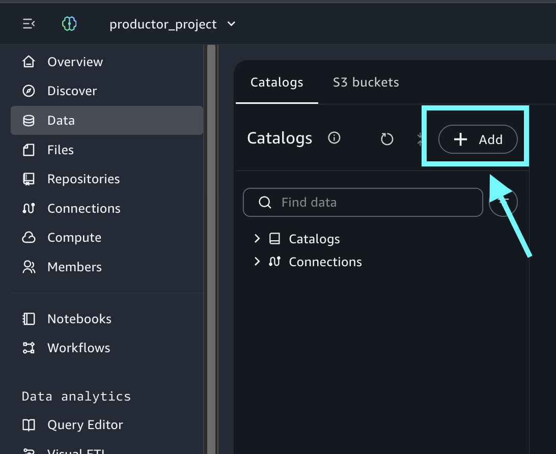
Clean up

The walkthrough creates querybook cells in your Query Editor session but doesn’t provision standalone infrastructure. To remove the generated SQL cells, delete them from your querybook or delete the querybook itself.

If you uploaded the California schools dataset specifically for this walkthrough, remove the following resources to avoid ongoing charges:

  • SageMaker Unified Studio domain. If you created a domain solely for this walkthrough, delete it to stop incurring charges. Refer to the SageMaker Unified Studio administration guide for deletion steps.
  • Uploaded tables. In the Data explorer, right-click each table you created and choose Delete table to remove the data from your project database and the underlying S3 storage.
  • Amazon Athena query results. Amazon Athena stores query results in an S3 output location. Delete the query result files from that bucket, or delete the bucket if you created it solely for this walkthrough.
  • Amazon CloudWatch logs. If Amazon Athena queries generated CloudWatch log groups, delete those log groups to avoid storage charges.

Conclusion

Data Agent in Query Editor brings conversational, catalog-aware SQL development to your Amazon Redshift and Amazon Athena workloads. In this post, you explored unfamiliar data, built a multi-step investment analysis, recovered from query errors, and summarized findings through natural language prompts.

Data Agent works within your existing IAM and AWS Lake Formation security controls, keeps your data within your AWS environment, and retains context across your analytical workflow so each question builds on the last.

Get started with these next steps:

  1. Run your first prompt. Open Query Editor in your SageMaker Unified Studio domain and enter Show me the top 10 tables in my catalog with the most columns. For setup, refer to the SageMaker Unified Studio getting started guide.
  2. Add descriptions to your AWS Glue Data Catalog. Table descriptions and column-level business metadata improve the quality of generated SQL. For best practices, refer to Populating the AWS Glue Data Catalog.
  3. Try a multi-step analysis. Enter Which product categories had declining revenue quarter-over-quarter, and which regions drove the decline? and review Data Agent’s plan step by step.

For more information, refer to the Amazon SageMaker Data Agent documentation, the What’s New blog post, Amazon Redshift documentation, and Amazon Athena documentation. To learn how Data Agent works in notebooks, refer to Accelerate context-aware data analysis and ML workflows with Amazon SageMaker Data Agent.


About the authors

Jason Ramos

Jason Ramos

Jason is a Front-End Engineer on the Amazon SageMaker Unified Studio team. He builds the scalable frontend experiences that power SageMaker Data Agent, bringing conversational AI capabilities to data scientists, analysts, and engineers across SageMaker Unified Studio. Outside of work, he enjoys playing piano and exploring the Bay Area food scene.

Olena Mursalova

Olena Mursalova

Olena is a Software Development Engineer on the Amazon SageMaker Unified Studio team, where she develops the SageMaker Data Agent — an intelligent assistant that turns natural language prompts into code, visualizations, and data insights for data engineers and analysts.

Jessica Cheng

Jessica Cheng

Jessica is a Front-End Engineer on the Amazon SageMaker Unified Studio team based in the Bay Area, where she builds intelligent data agent experiences. At work, she is passionate about creating accessible, easy-to-use experiences at scale. Outside of work, her passions lie in finding the best swimming hole in California.

Sanjana Sekar

Sanjana Sekar

Sanjana is a Software Development Engineer on the Amazon SageMaker Unified Studio team. She was one of the engineers who built the SageMaker Data Agent, bringing conversational AI-powered SQL generation and debugging to Query Editor. She is focused on improving data agent capabilities and the compute blueprints experience within SageMaker Unified Studio. Outside of work, she enjoys hiking and biking.

Siddharth Gupta

Siddharth Gupta

Siddharth is heading Generative AI within SageMaker’s Unified Experiences. His focus is on driving agentic experiences, where AI systems act autonomously on behalf of users to accomplish complex tasks. An alumnus of the University of Illinois at Urbana-Champaign, he brings extensive experience from his roles at Yahoo, Glassdoor, and Twitch.

Schedule notebook runs in Amazon SageMaker Unified Studio

Post Syndicated from Shivani Mehendarge original https://aws.amazon.com/blogs/big-data/schedule-notebook-runs-in-amazon-sagemaker-unified-studio/

If you build notebooks for recurring tasks such as daily customer analysis, weekly report generation, or data quality checks in Amazon SageMaker Unified Studio, you’ve likely wanted to run them automatically on a schedule. Until now, there wasn’t a native way to do this. Teams had to manage orchestration separately, even though the interactive notebook experience was already in place. Now, notebook scheduling is available, so you can configure your production workloads to run automatically with minimal manual intervention.

In this post, we walk you through the new scheduling and orchestrating capabilities for notebooks in Amazon SageMaker Unified Studio. You will learn how to:

  • Trigger on-demand background runs, such as a model re-training job, without waiting at your desk.
  • Create recurring schedules for tasks such as nightly data freshness checks or weekly business reviews.
  • Parameterize notebooks so a single template can generate reports across different AWS Regions or customer segments.
  • Orchestrate multi-notebook workflows where one notebook’s output feeds into the next. For example, an extract, transform, and load (ETL) pipeline followed by a summary dashboard refresh.
  • Debug failed runs with AI-assisted troubleshooting.

Sample use case overview

In this walkthrough, you will take on the role of a logistics analyst who monitors shipping performance across carriers. The notebook loads shipping data from the ShippingLogs.csv dataset, identifies late deliveries, and generates a performance summary. You want to run this notebook every morning without manual intervention, reuse it across different carriers, and know when something goes wrong.

You will start by running a notebook in the background and viewing the results. Next, you will create a recurring schedule for daily runs, then parameterize the notebook to generate reports for different carriers. You will also orchestrate the notebook in a multi-step workflow and debug a failed run using AI-assisted troubleshooting.

Prerequisites

Before you begin, you need:

  • An Amazon SageMaker Unified Studio project with Notebooks enabled. See Set up IAM-based domains for permission requirements.
  • A sample dataset. We use the ShippingLogs.csv dataset, which contains shipping data including estimated and actual delivery times, carriers, and origins. You can download it from the Workshop Studio (the file is named ShippingLogs.csv on the linked page).

Setting up the notebook

Start by creating a new notebook in your SageMaker Unified Studio project. If you haven’t already, upload the ShippingLogs.csv file under the Shared tab in the Files panel.

SageMaker Unified Studio Notebook Files panel showing the Shared tab with the ShippingLogs.csv dataset uploaded

In the first cell, we load and explore the dataset. To reference the file in code, select the file in the Shared tab and copy the Amazon Simple Storage Service (Amazon S3) URI shown in the file details. Alternatively, you can reference it with this code:

import pandas as pd
from sagemaker_studio import Project

# Initialize the project
proj = Project()

# Get the S3 root path
s3_root = proj.s3.root

df = pd.read_csv(s3_root + '/ShippingLogs.csv')
df.head()

The dataset contains columns including Carrier, ActualShippingDays, ExpectedShippingDays, ShippingOrigin, ShippingPriority, and OnTimeDelivery. Add a second cell to analyze shipping performance for a single carrier:

import matplotlib.pyplot as plt

carrier_data = df[df['Carrier'] == 'GlobalFreight']
# Flag late deliveries
carrier_data['is_late'] = carrier_data['ActualShippingDays'] > carrier_data['ExpectedShippingDays']
late_pct = carrier_data['is_late'].mean() * 100
# Visualize actual vs expected shipping days
plt.figure(figsize=(12, 4))
plt.hist(carrier_data['ActualShippingDays'] - carrier_data['ExpectedShippingDays'], bins=20, edgecolor='black')
plt.axvline(x=0, color='red', linestyle='--', label='On time')
plt.title(f'Shipping Delay Distribution - GlobalFreight ({late_pct:.1f}% late)')
plt.xlabel('Days Over Expected')
plt.ylabel('Number of Shipments')
plt.legend()
plt.show()

With the notebook working interactively, you’re ready to automate it.

Running a notebook asynchronously

To trigger an asynchronous run, open your notebook. In the notebook header, choose the menu on the Run all button, and then choose Run in background.

Notebook header with the Run all menu expanded, showing the Run in background option

This captures a snapshot of the notebook in its current state and starts a run on a separate dedicated compute. You can continue working on other tasks or close the browser entirely. Your interactive session isn’t affected.

You will see a notification at the bottom of your screen confirming that the run started. To check the status of your run, choose View Run in the notification. This opens a view showing every background and scheduled run with its status, duration, and a link to view the full output.

Run history view showing background and scheduled runs with status, duration, and output links

You can choose to view the run details at any point to view results as cells run. The run details include three tabs:

  • Output: The notebook in read-only mode with cell results rendered, including dataframe outputs, visualizations, and print statements.
  • Parameters: The parameter values used for this run.
  • Logs: Run logs for debugging.

Run details view showing the Output, Parameters, and Logs tabs with rendered cell output

You can also access past runs by selecting the View Runs option in the notebook header.

Notebook header with the View Runs option highlighted

Stopping an in-progress run

If you need to cancel a run, open the run, and choose Stop. The run terminates, and its status updates to reflect the cancellation.

Run detail view with the Stop button selected to terminate an in-progress run

What to know about background runs

Compute: Each background run uses its own dedicated compute, separate from your interactive session. Your interactive work isn’t interrupted.

Packages: The packages that you install through the notebook’s package manager will be available in your background runs. When you use !pip install in code cells, the asynchronous run installs those packages as well.

Local files: Background runs can’t access files stored locally in your notebook environment. Reference data from your project’s shared storage (Amazon S3) or connected data sources instead.

Startup time: Expect a few minutes of startup time while compute is provisioned and your environment is prepared.

Creating a recurring schedule

Now that you’ve confirmed asynchronous runs work correctly, you can automate the notebook on a schedule. Choose the schedule icon in the notebook header to open the schedule creation form.

Schedule creation form opened from the notebook header schedule icon

Configure the following settings:

  • Schedule name: Enter a descriptive name, such as Daily Shipping Report.
  • Schedule type: Choose Recurring for repeated runs or One-time for a single future run.
  • Frequency: Define how often the notebook runs using a rate (for example, every one day) or a cron expression. Set the time zone and the start and end dates for the schedule. For example, set the schedule to run every day at 7:00 AM UTC starting tomorrow.
  • Flexible time window (optional): The number of minutes after the scheduled start time within which the run can be invoked. For example, with a 5-minute window, the notebook runs within 5 minutes of the start time.
  • Advanced settings:
    • Compute Instance: Keep the current settings or override with a different instance type for the asynchronous run to use.
    • Timeout: Set a maximum run duration to help prevent notebooks from running indefinitely. If left blank, it defaults to 60 minutes.

Choose Create.

Configured schedule form with name, recurring type, daily frequency, and advanced settings populated

The schedule appears in the Schedules tab of the activity panel. SageMaker Unified Studio creates an Amazon EventBridge Scheduler schedule for each schedule you configure.

Schedules tab in the activity panel listing the newly created Daily Shipping Report schedule

Viewing schedule run history

To view past runs for a schedule, choose the schedule name in the Schedules activity panel. This opens the schedule details view, where you can see the list of runs triggered by that schedule, the duration of each run, and a link to open the notebook output for an individual run.

Schedule details view showing the list of past runs with status, duration, and output links

Editing and deleting schedules

To modify a schedule, choose Edit next to it in the Schedules panel. You can change the frequency, instance type, timeout, and other configuration fields. To pause or resume a schedule, choose Pause or Resume from the same menu. To remove a schedule, choose Delete from that menu. Deleting a schedule stops future runs but preserves historical run outputs in Amazon S3 for auditing purposes.

Schedules panel with the Edit, Pause, Resume, and Delete options for a schedule

Parameterizing notebooks

With parameters, you can reuse a single notebook across different inputs without duplicating code. For example, you can run the same shipping performance report for each carrier by passing a different carrier name to each run.

Defining parameters

Open the Parameters activity panel and choose Add. Set the parameter name to carrier and the default value to GlobalFreight.

Parameters activity panel with the carrier parameter and GlobalFreight default value configured

Using parameters in code

In your notebook, replace the second cell with the following code. This retrieves the carrier parameter value using the SageMaker Unified Studio Python SDK instead of the hardcoded value:

import sagemaker_studio
import matplotlib.pyplot as plt

carrier = sagemaker_studio.nbutils.parameters.get("carrier")

carrier_data = df[df['Carrier'] == carrier].copy()
carrier_data['is_late'] = carrier_data['ActualShippingDays'] > carrier_data['ExpectedShippingDays']
late_pct = carrier_data['is_late'].mean() * 100

plt.figure(figsize=(12, 4))
plt.hist(carrier_data['ActualShippingDays'] - carrier_data['ExpectedShippingDays'], bins=20, edgecolor='black')
plt.axvline(x=0, color='red', linestyle='--', label='On time')
plt.title(f'Shipping Delay Distribution - {carrier} ({late_pct:.1f}% late)')
plt.xlabel('Days Over Expected')
plt.ylabel('Number of Shipments')
plt.legend()
plt.show()

Creating schedules with different parameter values

Now create three schedules for the same notebook, each targeting a different carrier:

  • “daily-shipping-gf” with carrier = GlobalFreight.
  • “daily-shipping-mc” with carrier = MicroCarrier.
  • “daily-shipping-shipper” with carrier = Shipper.

When you view a historical run, a separate Parameters tab in the run output displays the parameter values that were active for that run.

You can also override parameter values when triggering an on-demand background run. Choose the menu on the Run all button, then choose Run with settings. You can keep the defaults or provide custom values for that run.

Orchestrating with Workflows

To combine notebooks into a multi-step pipeline, such as running a data calculation notebook before the shipping log notebook, you can use the Notebook Operator in the Workflows tool to orchestrate them.

To do this, choose the Add to workflows button under the options menu of the notebook header.

Notebook header options menu with the Add to workflows button highlighted

This takes you to the Workflows tool, adding a new Notebook Operator task with prefilled properties from your notebook. When configuring the Operator task:

  • Select the target notebook from the notebook menu.
  • Use the Parameters widget to pass notebook parameters into the run of the notebook.
  • Specify optional arguments such as the compute instance and timeout configuration for the run.

Workflows canvas with a Notebook Operator task configured with notebook, parameters, and compute settings

Workflows also supports polling for the status of a notebook run for a particular notebook using Notebook Sensor. In Workflows, you can add a new Sensor task by hovering on the edge of the existing Operator task, where a plus (+) button is displayed.

Workflows canvas showing the plus button on the edge of an Operator task for adding a Sensor

You can then search for and add the Notebook Sensor to the canvas.

Task picker dialog with Notebook Sensor selected for adding to the workflow canvas

When configuring the Sensor task, specify the notebook run ID within the text field. The Operator’s form field contains Jinja templating to retrieve the notebook run. If the Sensor is used within the same workflow as the Operator, this template can be copied to use within a Sensor to poll the notebook run. Select the target notebook from the notebook menu.

Notebook Sensor configuration panel with the notebook run ID field populated using Jinja templating

Within Workflows, you can configure notebook runs to emit outputs and use those outputs as inputs for subsequent notebook runs.

Building off of the previous shipping log notebook example, we will pass the carrier parameter from an upstream notebook’s output. Your shipping-logs-analysis notebook should be already set up.

Because the notebook depends on the carrier parameter, you can specify it in the Parameters panel.

Parameters panel for the shipping-logs-analysis Operator with the carrier parameter dependency configured

Now, define a second notebook, calculate-best-carrier, which performs a calculation to determine our best carrier to use for shipping:

import pandas as pd
from sagemaker_studio import Project

# Initialize the project
proj = Project()

# Get the S3 root path
s3_root = proj.s3.root

df = pd.read_csv(s3_root + '/ShippingLogs.csv')
df.head()

carrier_stats = df.groupby('Carrier').agg(
    total=('OrderID', 'count'),
    late=('OnTimeDelivery', lambda x: (x == 'Late').sum())
).reset_index()
carrier_stats['late_pct'] = carrier_stats['late'] / carrier_stats['total'] * 100

best = carrier_stats.sort_values('late_pct', ascending=True).iloc[0]
best_carrier = best['Carrier']

print("Late % by carrier:")
print(carrier_stats.to_string(index=False))
print(f"\nBest carrier: {best_carrier} ({best['late_pct']:.1f}% late)")

To configure the calculate-best-carrier notebook’s outputs, you can choose the Variables panel. A new selector is available at the bottom of this panel which allows you to select variables to mark as outputs.

Variables panel with the selector at the bottom for marking notebook variables as outputs

We want this notebook to emit the best_carrier variable.

Variables panel showing best_carrier marked as an output variable for the calculate-best-carrier notebook

Now, use the Add to workflows button as previously demonstrated to quickly add this notebook within a workflow. Chain a second Notebook Operator that points to our shipping-logs-analysis notebook. Because we specified a parameter dependency on carrier for this notebook, it’s available as an option in the Parameters widget menu.

Parameters widget menu of a Notebook Operator showing carrier as a configurable parameter dependency

When they’re chained, the notebook tasks detect the outputs set in upstream notebook runs. These outputs can be selected as keys within the Parameters widget of the Operator to pass into the run. This can be done recursively for an arbitrary number of Operator tasks. We can select the emitted best_carrier output from the calculate-best-carrier notebook.

Parameters widget displaying best_carrier as a selectable upstream output to pass into the next Operator

You can now choose the Save button on the top left of the visual canvas and the Run button to start the workflow. When the workflow is completed, the specified notebook outputs are available in the Task Output panel and the notebook run result can be viewed in the Notebooks tool.

Task Output panel showing the emitted notebook outputs after a successful workflow run

Notebook run result rendered in the Notebooks tool after the chained workflow completes

In a similar manner, the Notebook Sensor will also emit the notebook outputs from a particular notebook’s run which can be used within other tasks. This is useful when you want to retrieve outputs from a notebook run in another workflow.

Debugging a failed run with AI assistance

When viewing your past runs, you notice that a run from earlier today has a Failed status. Choose the failed run to open the notebook output in read-only mode.

In this example, suppose you incorrectly referred to column name ActualShippingDays as DeliveryDays. The run would fail with a KeyError: 'DeliveryDays' in the cell that computes late deliveries.

At the top of the failed run output, choose Troubleshoot with AI. Choosing the Troubleshoot with AI button lands you in the notebook with the Agent chat panel open.

Failed run output with the Troubleshoot with AI button highlighted at the top of the page

The data agent analyzes the cell outputs, identifies the cell that errored, explains the root cause, and suggests a fix. In this case, it identifies that the column DeliveryDays doesn’t exist in the dataframe and suggests updating the code reference. You can review the change, then verify the fix by choosing Run in background from the Run all menu to trigger a test run before the next scheduled run.

Note: You can also use the Data Agent to create schedules and start notebook runs using natural language, without having to navigate.

Cleaning up

To avoid incurring future charges, delete the resources that you created in this walkthrough:

  • Delete any schedules that you created from the Schedules panel in your notebook.
  • Delete test notebooks if you don’t need them.
  • Navigate to the Workflows page and delete any workflows that you created during this walkthrough.
  • Your project’s Amazon S3 storage retains historical run outputs until you manually remove them.

Conclusion

In this post, we showed how to run notebooks in the background in Amazon SageMaker Unified Studio using background runs, schedules, parameterization, workflow orchestration, and AI-assisted debugging. Using a shipping logistics dataset, we demonstrated how a single notebook can be parameterized to generate performance reports for different carriers on independent schedules, all without duplicating code or managing extensive infrastructure.

To get started, open a notebook in your SageMaker Unified Studio project, choose the menu on the Run all button in the notebook header, and choose Run in background. For more advanced use cases, explore workflows in Amazon SageMaker Unified Studio to build multi-step data pipelines, or review the Amazon SageMaker Unified Studio User Guide for additional configuration options.

Learn more:

If you have feedback or questions, reach out on AWS re:Post for Amazon SageMaker Unified Studio.


About the authors

Shivani Mehendarge

Shivani Mehendarge

Shivani is a Software Development Engineer at Amazon Web Services, where she builds scalable infrastructure that helps data teams run and automate their workloads in Amazon SageMaker Unified Studio. She is passionate about solving complex distributed systems challenges and building reliable cloud services.

Regan Perk

Regan Perk

Regan is a Senior Software Development Engineer on the Amazon SageMaker Unified Studio team. She designs, implements, and maintains features that enable customers to manage schedules and workflows in SageMaker Unified Studio.

Qazi Ashikin

Qazi Ashikin

Qazi is a Software Development Engineer at Amazon Web Services, where he works on developing features that allow customers to orchestrate workflows and schedules in SageMaker Unified Studio. He also works on AWS Glue Studio, where he builds agentic systems and maintains services that enable data analytics.

How Amazon is moving to integrate catalogs to improve data discovery with Amazon SageMaker

Post Syndicated from Pradeep Misra original https://aws.amazon.com/blogs/big-data/how-amazon-is-moving-to-integrate-catalogs-to-improve-data-discovery-with-amazon-sagemaker/

Enterprises face challenges when teams create data assets outside of central data catalogs. It adds overhead for discovery, and limits collaboration. Amazon’s Business Data Technologies (BDT) team has built an enterprise data catalog (Andes) for sharing datasets under well-defined policies. However, teams created catalog of local datasets and other non-tabular assets such as dashboards and metrics, outside Andes. This made it difficult to discover all assets in a consolidated way.
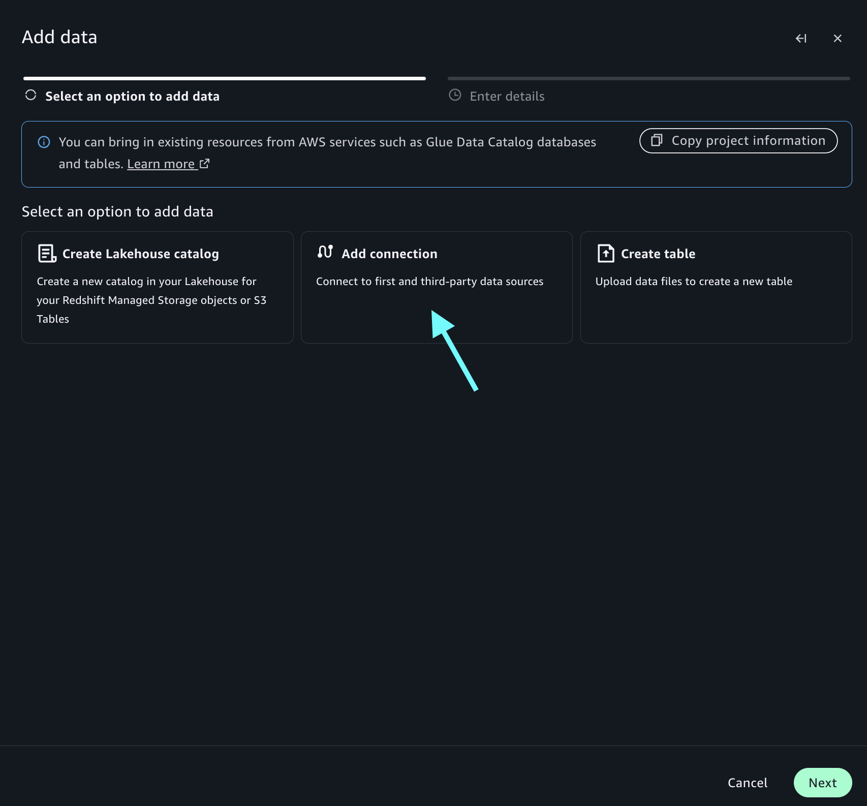
In this post, we share how Amazon.com is working to integrate catalogs by extending enterprise data catalog Andes with Amazon SageMaker.

Need for expanding catalog and governance from datasets to data assets

Without a single solution, users had to search multiple catalogs depending upon the asset type. Teams spent considerable time indexing the different catalogs and identifying the right one for their task. This slowed them down and took time away from solving the business problems.

To address these challenges, BDT team identified four critical capabilities needed:

  1. Multimodal catalog – Data consumers required the ability to blend enterprise data with local datasets and use them together for specific use cases. Teams sought to discover not only datasets, but also assets such as metrics, dashboards, and business files, to obtain a complete view of available resources. This necessitated a catalog that consolidates datasets and data assets in one location.
  2. Uniform governance and enforcement – To maintain best data protection practices and support business goals, teams need consistent enterprise-wide data governance where they request access once and the system enforces that access uniformly across all compute engines, alleviating fragmented or redundant access management. For internal systems, there was need for trusted identity propagation so user identity is preserved and used across AWS and internal systems for consistent enforcing.
  3. Multi-approval workflows – The solution supports multiple approval workflows within a single system, using Andes for dataset approvals and a custom workflow for dashboard approvals to maintain total governance and visibility across data assets.
  4. Delegated ownership – While enterprise teams retain overarching governance responsibility, business-specific data stewards required the ability to modify select attributes and apply appropriate tags to assets produced by their respective producers and consumers.

Solution: Unify datasets and data assets with Amazon SageMaker

Amazon chose to extend Andes with Amazon SageMaker to enhance the discovery experience. SageMaker offers native support for multimodal catalogs, and integrated with enterprise identity management, making it the ideal foundation for extending Andes’ governance model.

Rather than broadcasting assets across multiple domains, a single enterprise-wide domain standardizes and synchronizes data assets in one place. This domain is associated with AWS IAM Identity Center, which is connected to Amazon’s corporate identity system to maintain best data protection practices by limiting direct permissions and using corporate identity and group-based permissions.

Architecture diagram showing how Amazon SageMaker integrates with enterprise data catalog Andes and AWS IAM Identity Center

This integrated architecture directly addresses the identified challenges:

  • Single-pane asset discovery – Datasets and data assets are accessible through a single, consolidated view, avoiding the need to navigate across disparate systems or domains. This simplifies discovery and reduces the time to insight for teams across the organization.
  • Extended governance – Governance of both enterprise-wide and local datasets is orchestrated through a single system.
  • Extended observability – Trusted Identity Propagation (TIP) through AWS IAM Identity Center allows human users to access data interactively using their corporate identities. This provides audit-trail visibility into who is accessing what data for audits and organization’s observability requirements.
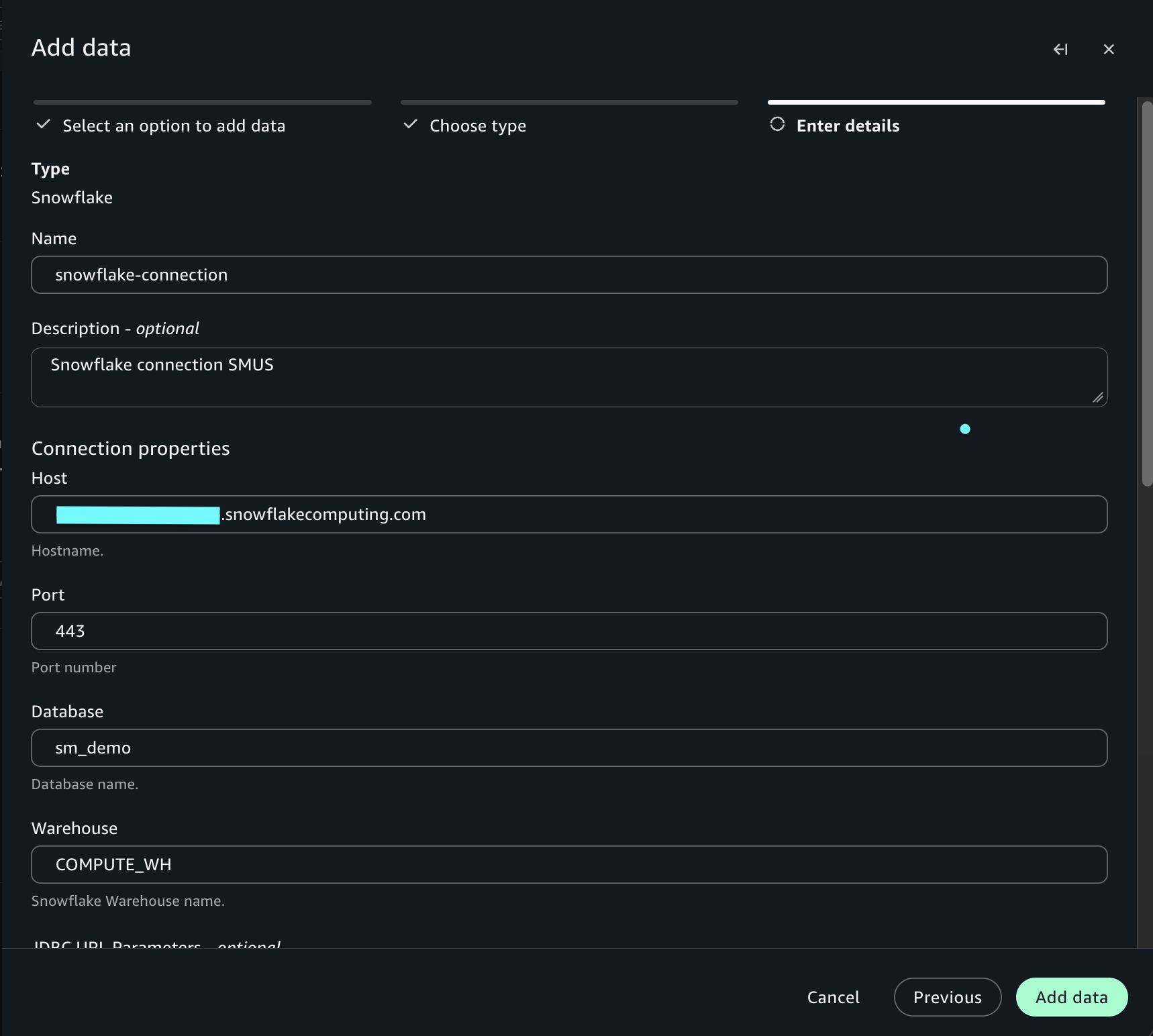
  • Amazon tool integration – Integration with Git and other internal systems automates management of accounts, permissions, and approvals. This reduces manual overhead and helps maintain that access controls remain tightly aligned with existing business workflows.

Design overview

This section describes the key features and design of the Amazon SageMaker integration. The technical implementation consists of three core components:

1) Catalog connectors

Amazon built connectors and ingestion paths to bring data assets into Amazon SageMaker while maintaining business continuity and preserving existing governance:

  • Andes integration: SageMaker provides APIs to synchronize assets from external catalogs. BDT extended this to bring Andes datasets (with their sophisticated metadata, business context) into the integrated experience. The integration preserves Andes’ permission model and governance workflows, to maintain existing security standards and best practices intact.
  • Account onboarding: Teams self-serve onboard their AWS accounts through an AWS Lambda-based integration. When creating projects, SageMaker queries this service to determine which accounts a user’s identity can access.

2) Delegated ownership

When data systems scale across business units, centralized governance teams need to delegate permissions for catalog enrichment, policy enforcement, and metadata management.

  • Catalog enhancement allows business teams to define and publish their own business glossaries, curated vocabularies of domain-specific terms, definitions, and relationships, directly within the catalog. Allowing business owners to author and maintain these glossaries increased accuracy and discoverability of catalog assets. Data consumers across the enterprise benefit from clearer, more consistent terminology.

3) Integration with consumption and access tooling

Teams discover data in SageMaker Unified Studio and consume it through both SageMaker Unified Studio and internal tooling:

  • Data discovery: SageMaker Unified Studio integrates with Amazon-wide Identity Center allowing almost all Amazon users to authenticate and search for cataloged assets. This integration addresses the data discovery problem by providing enterprise-wide visibility into available data resources.
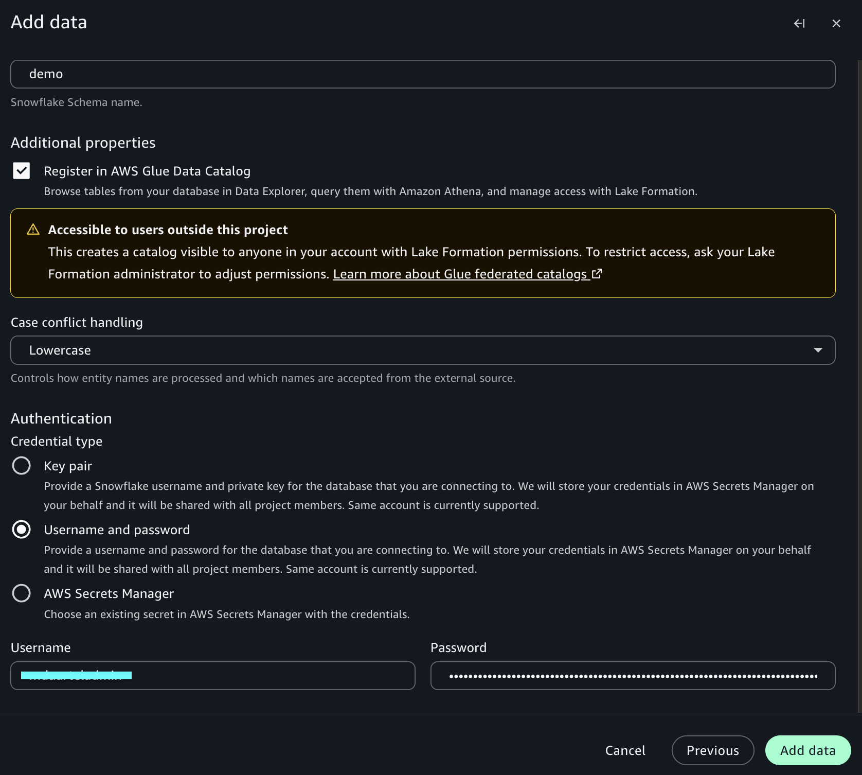
  • Integrated development environment: SageMaker Unified Studio provides built-in tooling out of the box including a Query Editor for SQL analytics and Amazon SageMaker AI for machine learning (ML), which helps teams access data, build models, and collaborate across organizational boundaries.
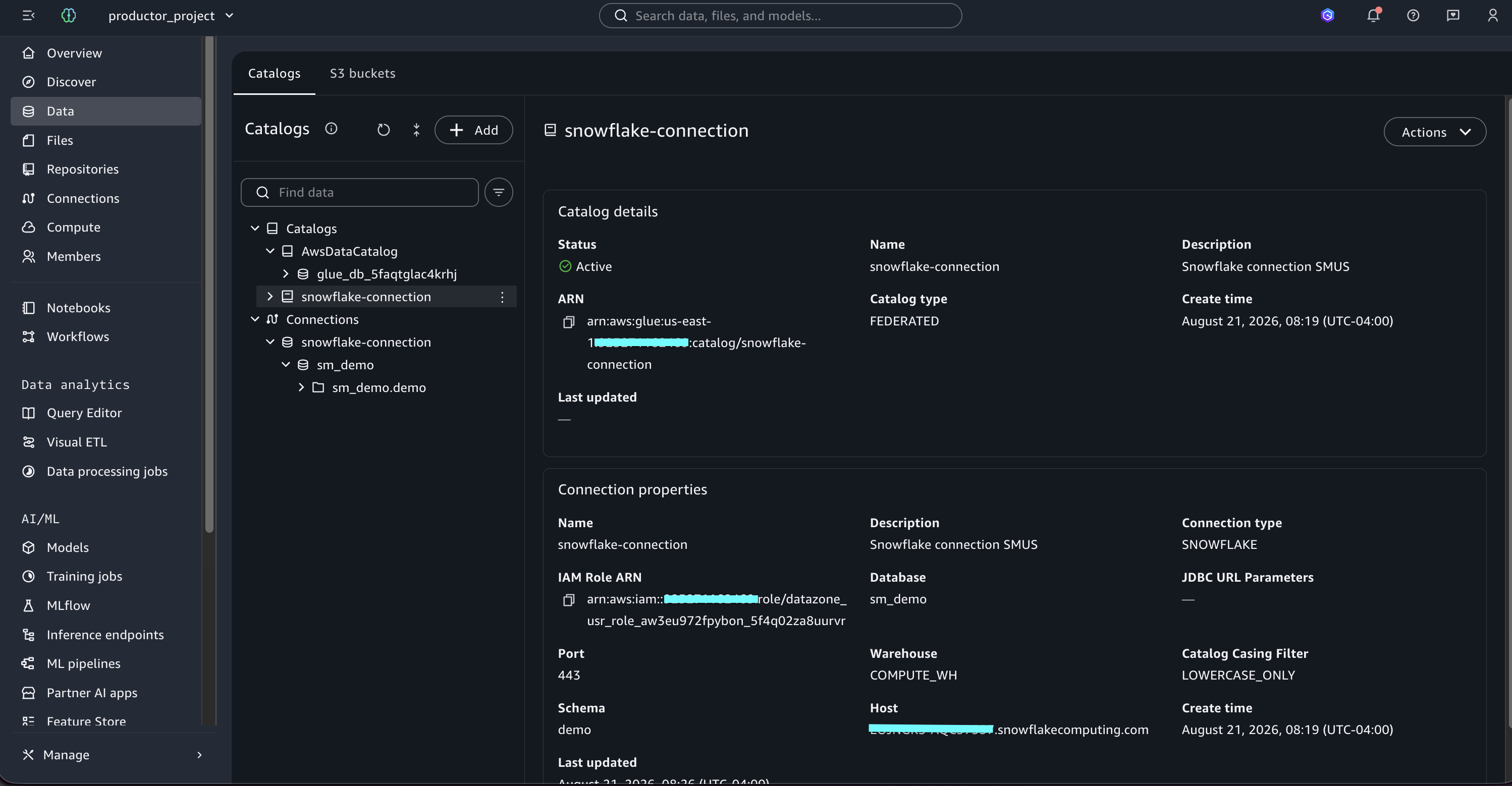
  • Code repository integration: Manage code with full Git operations supported from SageMaker Unified Studio. Query code and notebook code persist to GitFarm (Amazon’s internal Git system), allowing teams to view and manage their work through Amazon’s standard version control system.
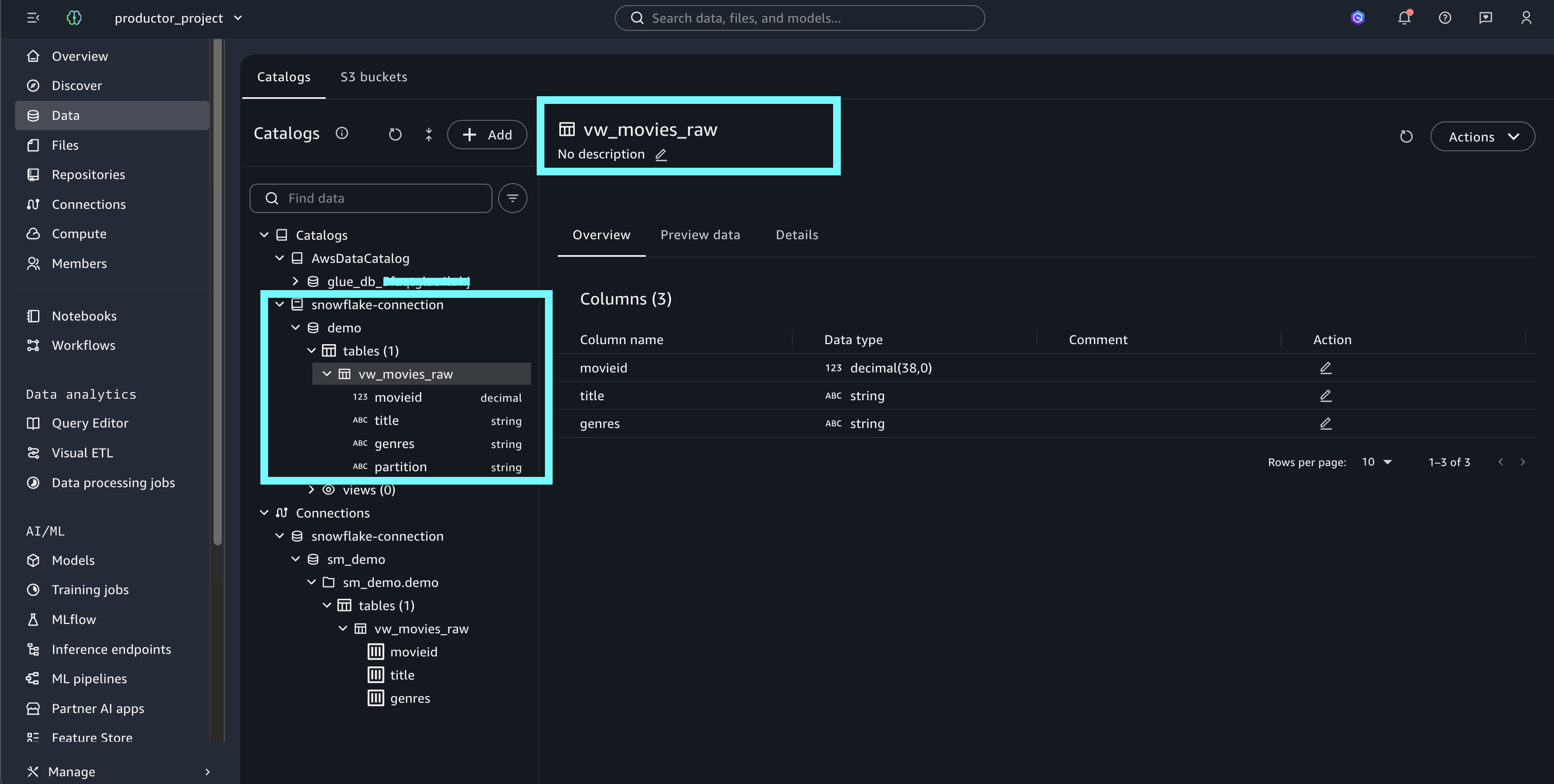
  • Native analytics integration: Projects directly connect to AWS analytics engines including Amazon Athena for SQL, AWS Glue and Amazon EMR for Apache Spark, and Amazon Redshift for data warehousing. User-authored jobs use Andes governance and permissions across engines for consistent access control.

SageMaker implementation results

SageMaker catalog now encompasses various types of data assets from across the organization, representing an expansion from datasets alone to a complete inventory of data, dashboards, metrics, models, and other data assets, all while maintaining best practices and appropriate access and use guardrails.

“SageMaker provides a unified catalog that makes discovery and sharing of data assets, metrics and dashboards across teams straightforward, with direct integration to Andes datasets. SageMaker delivers deep integration through Git repository connections and enterprise identity management that aligns with existing Amazon workflows.”

– Gerry Moses, Sr. Principal TPM, Amazon

  • Faster data discovery – Data consumers can go to one place to locate trusted, high-quality assets with significantly less friction, which reduces the time from question to insight. By surfacing well-documented, governed assets through an enriched catalog, teams can confidently identify the right data for their use cases without navigating sprawling, inconsistent inventories or relying on tribal knowledge.
  • Improved collaboration – Breaks down data silos by making curated assets discoverable and reusable across Amazon. When teams can build on shared, authoritative datasets rather than creating redundant copies, data proliferation is reduced.

Conclusion

By integrating their existing governance tooling with Amazon SageMaker to build a centralized data catalog, BDT is creating a foundation for faster, more efficient data discovery across teams. Amazon SageMaker helped unify diverse data types with their existing catalog and enabled collaboration across teams to help them find the right data. By integrating with existing governance frameworks, BDT demonstrates how organizations can expand their catalog capabilities while preserving existing enterprise investments.

To learn more and get started with Amazon SageMaker Unified Studio, visit aws.amazon.com/sagemaker/unified-studio or the AWS console.


About the authors

Matt David

Matt David

Matt is a Sr PMM, specializing in helping data teams with AI-powered analytics. His areas of interest include self-service analytics, data democratization, and preparing organizations for the age of AI agents. He brings extensive experience from his roles at Atlassian, Hex, and DataCamp.

Gerry Moses

Gerry Moses

Gerry is a Senior Principal Technical Program Manager in Business Data Technologies where he leads joint Amazon/AWS programs. His work improved data governance for Amazon’s Andes data lake, enabled broader AWS technology adoption by data lake users, and influenced product improvements that benefited all AWS customers.

Ramesh Singh

Ramesh Singh

Ramesh is a Senior Product Manager Technical at AWS in Seattle, Washington, currently with the Amazon SageMaker team. He is passionate about building high-performance ML/AI and analytics products that help enterprise customers achieve their critical goals using cutting-edge technology.

Pradeep Misra

Pradeep Misra

Pradeep is a Principal Analytics and Applied AI leader at AWS. He is passionate about solving customer challenges using data, analytics, and AI/ML. Outside of work, he likes exploring new places, trying new cuisines, and playing badminton with his family. He also likes doing science experiments, building LEGOs, and watching movies with his daughters.

Eunji Kang

Eunji Kang

Eunji is a Principal Product Manager Technical focusing on democratizing data across Amazon teams for fast data-driven business decisions without compromising security and compliance.

Trevor Gasdaska

Trevor Gasdaska

Trevor is a Principal Engineer focusing on data compliance and agentic AI workflows for Big Data Technologies at Amazon. He builds tools that help teams govern and use data at scale.

Brad Porter

Brad Porter

Brad is a Principal Business Development Manager at Amazon Web Services. He works with Amazon.com and enterprise customers to define and accelerate go-to-market strategies across Data Analytics, AI/ML, and Generative AI. He has over 20 years of experience in cloud strategy, enterprise infrastructure, and technology leadership.

Automate deployment of data and AI applications with Amazon SageMaker Unified Studio CI/CD CLI

Post Syndicated from Saurabh Bhutyani original https://aws.amazon.com/blogs/big-data/automate-deployment-of-data-and-ai-applications-with-amazon-sagemaker-unified-studio-ci-cd-cli/

Organizations building data and AI applications in Amazon SageMaker Unified Studio combine multiple AWS services, including AWS Glue, Amazon Athena, Amazon Managed Workflows for Apache Airflow (Amazon MWAA), Amazon SageMaker AI, and Amazon Quick Sight, into single applications. Promoting these applications from development to test and production stages requires substituting service-specific configurations for each stage and provisioning resources in the correct order.

Data teams understand which services their applications need but lack continuous integration and continuous delivery (CI/CD) expertise, while DevOps teams understand deployment automation but must learn each AWS service’s provisioning requirements.

The CI/CD CLI for Amazon SageMaker Unified Studio (aws-smus-cicd-cli) is an open source command line tool that automates deployment of multi-service data and AI applications across pipeline stages. Data teams define their application once in a YAML manifest, DevOps teams deploy with a single command, and the CLI handles configuration substitution, dependency ordering, and resource provisioning automatically. For details, see the CI/CD CLI documentation.

In this post, we walk through how the CI/CD CLI works, show you how to deploy a real application across environments, and demonstrate how it fits into your existing CI/CD workflows.

Customer spotlight

Bureau Veritas, a global leader in testing, inspection, and certification, operates across multiple SageMaker Unified Studio environments to support its data and AI teams. With their data and DevOps teams working on different parts of the application lifecycle, Bureau Veritas needed a controlled way to promote workloads from development through test to production while preserving clear ownership boundaries between the two teams.

“We need to promote data and AI applications across SageMaker Unified Studio environments in a controlled way that respects the boundaries between our data teams and our DevOps teams. The CI/CD CLI does exactly that — a single manifest from the data team, a single deploy command from DevOps, and full control over what goes to production.”

— Gilles Kempf, Architecture Manager, Bureau Veritas

How the CI/CD CLI works

The CI/CD CLI introduces a clean separation of concerns between data teams and DevOps teams.

Data teams define what to deploy in a declarative YAML manifest (manifest.yaml). The manifest describes the application’s resources, including AWS Glue extract, transform, and load (ETL) jobs, Athena queries, Airflow directed acyclic graphs (DAGs), Quick Sight dashboards, and SageMaker training jobs, along with stage-specific configurations for each environment.

DevOps teams define how and when to deploy using their existing CI/CD systems. They retain full control over their deployment methodology. They choose whether to promote content through git branches, a bundle artifactory, or both; they decide the shape of the pipeline, including which stages to include (dev, staging, pre-prod, prod) and which manual approvals or security gates are required. They run aws-smus-cicd-cli deploy inside GitHub Actions, Jenkins, or GitLab CI workflows without needing to understand which AWS services the application uses or how SageMaker Unified Studio projects are structured. The CLI is a utility for AWS analytics service deployment, not a CI/CD methodology. Your team’s existing conventions for branches, approvals, and pipeline shape stay exactly as they are.

The CLI is the abstraction layer between the two. It reads the manifest, substitutes stage-specific configurations (S3 paths, AWS Identity and Access Management (IAM) roles, account IDs, and connection strings), provisions resources in dependency order, and handles all AWS service interactions.The following diagram illustrates this separation:

SageMaker CI/CD

Key concepts

Application manifest

Each stage maps to a dedicated SageMaker Unified Studio project. This one-stage-to-one-project mapping is the foundation of CI/CD isolation: each project has its own domain, IAM boundaries, connections, and data, so changes in dev can never affect prod. For stronger isolation, projects can span different AWS accounts and AWS Regions. For example, dev in a sandbox account and prod in a production account in a different Region. Because each stage is a real SageMaker Unified Studio project, teams can open it in the console at any time to observe workflows, inspect resources, and troubleshoot deployments. Project membership is managed per project, so you control exactly who has access to each stage. For example, developers in dev and a release team in prod.The manifest file is the single source of truth for your application. It declares:

  • Content: application code from git repositories, data files from S3, Quick Sight dashboards, and workflow definitions.
  • Stages: environment-specific project mappings (dev, test, prod, etc.), each isolated as described earlier.
  • Configuration: stage-specific settings that are substituted automatically at deploy time.

Here is an example manifest for an analytics application with AWS Glue ETL and Quick Sight:
applicationName: SalesAnalyticsDashboard

content: 
  storage: 
    - name: etl-code 
      include: ["*.py"] 
    - name: workflows 
      include: ["*.yaml"] 
  quicksight: 
    - name: SalesDashboard 
      type: dashboard 
  workflows: 
    - workflowName: sales_etl_pipeline 
      connectionName: default.workflow_serverless 
 
stages: 
  dev: 
    domain: 
      region: us-east-1 
    project: 
      name: analytics-dev 
    deployment_configuration: 
      storage: 
        - name: etl-code 
          connectionName: default.s3_shared 
          targetDirectory: sales/bundle/etl 
        - name: workflows 
          connectionName: default.s3_shared 
          targetDirectory: sales/bundle/workflows 
 
  prod: 
    domain: 
      region: us-west-2 
    project: 
      name: analytics-prod 
    deployment_configuration: 
      storage: 
        - name: etl-code 
          connectionName: default.s3_shared 
          targetDirectory: sales/bundle/etl 
        - name: workflows 
          connectionName: default.s3_shared 
          targetDirectory: sales/bundle/workflows 
      quicksight: 
        assets: 
          - name: SalesDashboard 
            owners: 
              - arn:aws:quicksight:${AWS_REGION}:${AWS_ACCOUNT_ID}:user/default/Admin/* 

Each stage must map to a separate SageMaker Unified Studio project, providing full isolation between environments. The CLI substitutes variables like ${AWS_ACCOUNT_ID} and ${AWS_REGION} at deploy time based on the target environment.

Bundles

A bundle is an immutable, versioned archive of your application. The bundle command reads from a source stage (typically dev) and packages the application code, workflow definitions, and resolved configurations into a self-contained artifact. The deploy command then applies that artifact to one or more target stages (test or prod).

This stage-to-bundle-to-stage promotion model supports controlled rollout through quality gates:

# Package from dev 
aws-smus-cicd-cli bundle --manifest manifest.yaml 
 
# Deploy to test 
aws-smus-cicd-cli deploy --manifest app.tar.gz --targets test 
 
# Validate the test deployment 
aws-smus-cicd-cli test --manifest manifest.yaml --targets test 
 
# Promote the same bundle to prod 
aws-smus-cicd-cli deploy --manifest app.tar.gz --targets prod 

The same artifact is deployed at every stage without rebuilding, providing audit trails and reproducible deployments for regulated industries.
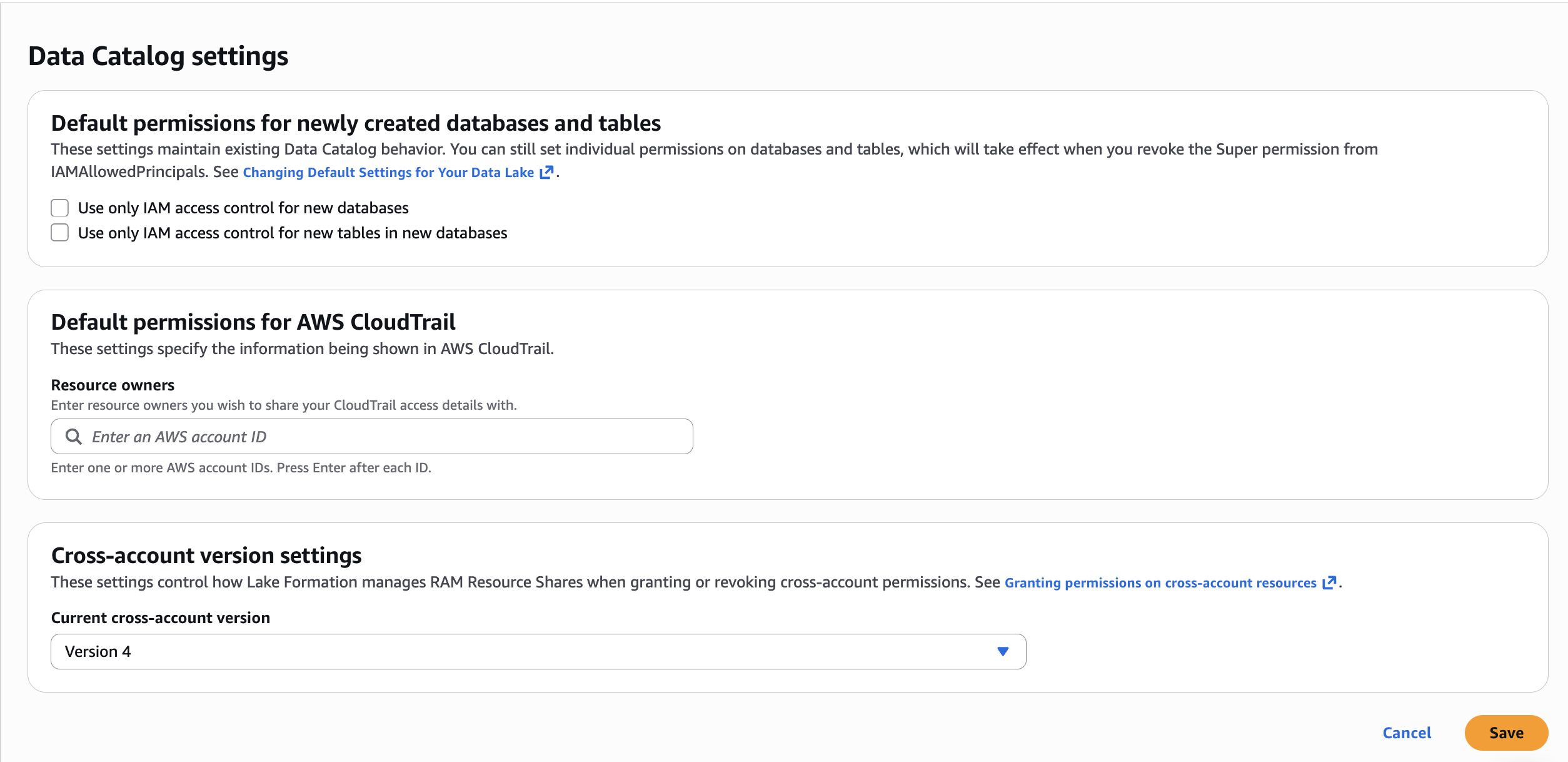
SageMaker Catalog integration

The CLI manages Amazon SageMaker Catalog resources as part of the deployment process. You can define catalog assets, glossaries, glossary terms, form types, asset types, and metadata forms, in your manifest. During deployment, the CLI searches for assets in the catalog, creates subscription requests for required data access, and waits for approval before proceeding. This automates the data governance workflow that teams previously handled manually.

CLI commands

The CI/CD CLI provides commands that cover the full deployment lifecycle:

Command Description
describe Validates the manifest, checks that target projects exist, and confirms the execution role has required permissions. Use –connect to validate against live AWS environments.
bundle Reads from a source stage and packages application code, workflow definitions, and configurations into an immutable, versioned archive.
deploy Applies bundle contents to one or more target stages. Provisions resources in dependency order.
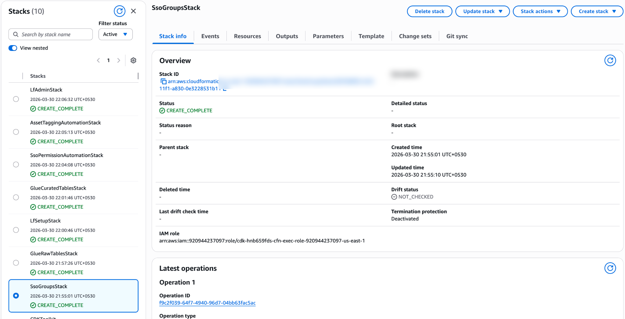
test Runs post-deployment validation to confirm services are running and ready for workloads.

create Generates a starter manifest from an existing SageMaker Unified Studio project.
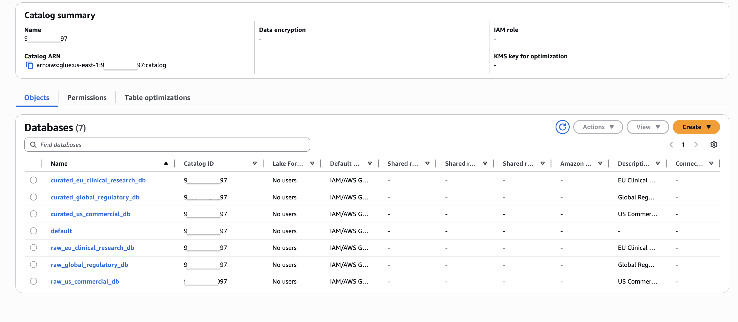
run Triggers Airflow workflow execution on MWAA or Airflow Serverless connections.
monitor Monitors workflow execution status in real time.
logs Fetches and streams workflow execution logs.
destroy Removes deployed resources and projects for cleanup or failure recovery.

Walkthrough: deploying a Quick Sight dashboard with AWS Glue ETL

In this section, we walk through deploying an analytics application that uses AWS Glue for ETL, Athena for queries, and Quick Sight for dashboards. This example is available in the GitHub repository.

Use case

An analytics team owns a Sales Analytics Dashboard built on AWS Glue ETL, Athena, and Quick Sight. They want to promote changes from a development environment to production with reproducible builds, automated validation, and a clear approval gate between stages, without writing custom deployment scripts or exposing data engineers to AWS provisioning details.

Solution overview

We use a sample application from the CI/CD CLI GitHub repository that includes AWS Glue ETL scripts, an Airflow workflow definition, a Quick Sight dashboard bundle, and integration tests. A single manifest.yaml describes the application and its dev and prod stages. The CLI handles the full lifecycle: bundle the app from dev, deploy it to test, run validation, and promote the same immutable artifact to prod.

Prerequisites

Before you begin, make sure you have the following:

Solution architecture

Each stage in the manifest maps to a dedicated SageMaker Unified Studio project (see the separation-of-concerns diagram in “How the CI/CD CLI works” earlier in this post). At deploy time, the CLI uploads ETL scripts and workflow definitions to the project’s S3 storage connection, provisions the Airflow workflow in MWAA Serverless, runs the workflow to create AWS Glue jobs and databases, and imports the Quick Sight dashboard. The same bundle artifact is applied to every downstream stage, ensuring dev, test, and prod stay in sync while remaining fully isolated.

Solution implementation

Step 1: Install the CLI

Install the CLI from PyPI:

pip install aws-smus-cicd-cli

Step 2: Create or customize a manifest

Clone the repository and start from the analytics example:

git clone https://github.com/aws/CICD-for-SageMakerUnifiedStudio.gitcd CICD-for-SageMakerUnifiedStudio/examples/analytic-workflow/dashboard-glue-quick

The example includes AWS Glue ETL scripts, an Airflow workflow definition, a Quick Sight dashboard bundle, and integration tests. Open manifest.yaml and update the project, domain, and deployment_configuration values under each stage so they match your own SageMaker Unified Studio projects and connection names.Alternatively, generate a manifest from an existing project: aws-smus-cicd-cli create --domain-id <your-domain-id> --dev-project-id <your-project-id>

Step 3: Validate your configuration

Run the describe command with --connect to verify your environment is ready. This connects to your AWS environment and validates that target projects exist, the execution role has the required permissions, and connections are reachable. Fix any issues before deploying.

aws-smus-cicd-cli describe --manifest manifest.yaml --connect

Step 4: Deploy

Run the deployment:

aws-smus-cicd-cli deploy --targets test --manifest manifest
During deployment, the CLI:
  1. Uploads ETL scripts and workflow definitions to S3 using the project’s storage connection.
  2. Creates the Airflow workflow in MWAA Serverless.
  3. Runs the workflow, which provisions AWS Glue jobs, creates databases, and runs ETL transformations.
  4. Imports the Quick Sight dashboard and refreshes datasets with the latest data.
  5. Processes any catalog asset subscriptions defined in the manifest.

Step 5: Validate

Run post-deployment validation to confirm services are running and ready for workloads:

aws-smus-cicd-cli test --manifest manifest.yaml --targets test

Step 6: Promote to production

Promote the same bundle artifact that was validated in the test stage to production. This guarantees the exact same artifact runs in prod:

# Promote the same bundle that was validated in test to prod

aws-smus-cicd-cli deploy --manifest app.tar.gz --targets prod

Integrating with GitHub Actions

The CLI works with existing CI/CD solutions. The GitHub repository includes reusable workflow templates that DevOps teams can adopt directly.The following is an example of a GitHub Actions workflow that implements a full bundle-based deployment pipeline:

name: Deploy Analytics Application 
on: 
  push: 
    branches: [main] 
 
jobs: 
  deploy-test: 
    runs-on: ubuntu-latest 
    steps: 
      - uses: actions/checkout@v4 
 
      - name: Install CLI 
        run: pip install aws-smus-cicd-cli 
 
      - name: Configure AWS credentials 
        uses: aws-actions/configure-aws-credentials@v4 
        with: 
          role-to-assume: ${{ secrets.AWS_ROLE_ARN }} 
          aws-region: us-east-1 
 
      - name: Validate 
        run: aws-smus-cicd-cli describe --manifest manifest.yaml --connect 
 
      - name: Bundle 
        run: aws-smus-cicd-cli bundle --manifest manifest.yaml 
 
      - name: Deploy to test 
        run: aws-smus-cicd-cli deploy --targets test --manifest manifest.yaml 
 
      - name: Run tests 
        run: aws-smus-cicd-cli test --manifest manifest.yaml --targets test 
 
  deploy-prod: 
    needs: deploy-test 
    runs-on: ubuntu-latest 
    environment: production 
    steps: 
      - uses: actions/checkout@v4 
 
      - name: Install CLI 
        run: pip install aws-smus-cicd-cli 
 
      - name: Configure AWS credentials 
        uses: aws-actions/configure-aws-credentials@v4 
        with: 
          role-to-assume: ${{ secrets.AWS_PROD_ROLE_ARN }} 
          aws-region: us-west-2 
 
      - name: Deploy to production 
        run: aws-smus-cicd-cli deploy --targets prod --manifest manifest.yaml

The CLI also works with Jenkins, GitLab CI, and Azure DevOps. See the CI/CD integration guide for additional examples.

In the next section, we cover which AWS services and workload types the CLI supports.

Supported workloads

The CLI deploys applications that span the following AWS services through Airflow workflow definitions:

  • Analytics and BI: AWS Glue ETL jobs and crawlers, Amazon Athena queries, Amazon Quick Sight dashboards, Amazon EMR jobs, Amazon Redshift queries.
  • Machine learning: SageMaker training jobs, ML model endpoints, SageMaker AI Pipelines.
  • Code and workflows: Jupyter notebooks, Python scripts, Airflow DAGs (MWAA and MWAA Serverless).
  • Data and storage: S3 data files, Git repositories, SageMaker Catalog resources (glossaries, glossary terms, form types, asset types, assets, data products, metadata forms).

The examples directory includes working applications for each of these patterns, with manifests, workflow definitions, and integration tests.

Failure recovery

If a deployment fails, the CLI stops at the point of failure and reports the error with a detailed stack trace. To recover:

  1. Run aws-smus-cicd-cli describe --connect to check which resources exist and which permissions are missing.
  2. Fix the issue and rerun aws-smus-cicd-cli deploy.
  3. For bundle-based deployments, redeploy a previous bundle version.
  4. Use aws-smus-cicd-cli destroy --targets <target> --force to clean up a failed deployment.

For detailed rollback procedures, see the Rollback Guide.

Conclusion

In this post, you learned how the Amazon SageMaker Unified Studio CI/CD CLI gives data and DevOps teams a clean separation of concerns: data teams describe their application once in a YAML manifest, and DevOps teams deploy it with a single command through their existing CI/CD pipelines. You saw how stages map to isolated SageMaker Unified Studio projects (optionally spanning AWS accounts and Regions), how bundles provide immutable, reproducible promotion through test and production, and how the CLI integrates with GitHub Actions, Jenkins, GitLab CI, and Azure DevOps. You also walked through deploying a Glue-and-Quick-Sight analytics application from dev through to prod.

Get started

The CI/CD CLI is available at no additional cost in all AWS Regions where Amazon SageMaker Unified Studio is available. You pay only for the underlying AWS resources provisioned during deployment.

Use the following steps to try it out:

  1. Install the CLI:
    pip install aws-smus-cicd-cli
  2. Browse the example applications for analytics and ML patterns.
  3. Follow the CI/CD CLI documentation to deploy your first application in 10 minutes.
  4. Review the Admin Guide for infrastructure setup.

For feedback and bug reports, open an issue on the GitHub repository.


About the authors

Ramesh H Singh

Ramesh H Singh

Ramesh H Singh is a Senior Product Manager Technical (External Services) at AWS in Seattle, Washington, currently with the Amazon SageMaker team. He is passionate about building high-performance ML/AI and analytics products that help enterprise customers achieve their critical goals using cutting-edge technology.

Vasudevan Venkataramanan

Vasudevan Venkataramanan

Vasudevan Venkataramanan is a Senior Software Engineer on the Amazon SageMaker Unified Studio team. He is responsible for technical direction of scheduling and orchestration within SageMaker Unified Studio. Outside of his professional work, he enjoys spending time with his kid, and playing pickleball and cricket.

Amir Bar Or

Amir Bar Or

Amir Bar Or is a Senior Software Engineer on the Amazon SageMaker Unified Studio team. He is responsible for technical direction of scheduling and orchestration within SageMaker Unified Studio. Outside of his professional work, he enjoys spending time with his kid, and playing pickleball and cricket.

Nikita Arbuzov

Nikita Arbuzov

Nikita is Software Engineer on the Amazon SageMaker Unified Studio team. He is responsible for building support for CI/CD features within SageMaker Unified Studio.

Saurabh Bhutyani

Saurabh Bhutyani

Saurabh Bhutyani is a Principal Analytics Specialist Solutions Architect at AWS. He is passionate about new technologies. He joined AWS in 2019 and works with customers to provide architectural guidance for running generative AI use cases, scalable analytics solutions and data mesh architectures using AWS services like Amazon Bedrock, Amazon SageMaker Unified Studio, Amazon EMR, Amazon Athena, AWS Glue, AWS Lake Formation, and Amazon DataZone.

Capture data lineage of Amazon EMR spark jobs into Amazon SageMaker Unified Studio

Post Syndicated from Jose Romero original https://aws.amazon.com/blogs/big-data/capture-data-lineage-of-amazon-emr-spark-jobs-into-amazon-sagemaker-unified-studio/

Data engineers running Apache Spark jobs on Amazon EMR face a persistent challenge: understanding how data moves through Spark pipelines as it’s transformed, joined, and written to downstream tables . Tracking these transformations manually requires examining job logs, reviewing code, and piecing together transformation logic across multiple sources. As pipelines scale, this process becomes complex. The visibility gap affects key business activities: troubleshooting data quality issues takes longer – impact analysis for schema changes requires more effort – and compliance audits need extensive documentation of data provenance.

Amazon SageMaker is the center for all your data and analytics where you can find and access all the data in your organization and act on it using tools across various use case. This unified platform addresses the data visibility challenge by bringing together data governance, collaboration, and discovery into a single interface. At the heart of this platform is Amazon SageMaker Catalog, a centralized hub that enables organizations to catalog, govern, and discover all their data assets with complete visibility into lineage. By capturing data lineage across your entire data ecosystem from raw sources through transformations to final outputs, SageMaker Catalog enables you to track data provenance across your entire platform, enable collaboration with clear visibility into data ownership and quality metrics, build trust through comprehensive data lineage that supports compliance and confident decision-making, and accelerate discovery of trustworthy, governance-ready data assets. You can access and visualize this lineage directly in Amazon SageMaker Unified Studio, which serves as the unified interface to explore data relationships and collaborate across your analytics workflows.

Amazon EMR, starting from version 7.11, now includes native OpenLineage support that automates lineage capture. OpenLineage is an open-source framework for data lineage that automatically emits lineage metadata from your data transformation jobs directly into Amazon SageMaker Catalog, or other data governance solutions, without requiring customizations.

This EMR native support of OpenLineage is part of a growing set of integrations across AWS analytics services including AWS Glue, Amazon EMR Serverless, and Amazon Redshift. The complete list of services with native OpenLineage integration can be found in the data lineage support matrix.

In this post, you’ll walk through a practical, step-by-step example that shows how to capture and track data lineage from Spark jobs running on Amazon EMR directly into Amazon SageMaker Catalog using OpenLineage. You’ll see how lineage metadata flows automatically and explore data relationships and dependencies across your workflows in Amazon SageMaker Unified Studio.

Solution overview

Imagine you’re part of a large enterprise that relies on HR analytics to optimize workforce planning, compensation strategies, and talent retention practices. Your data engineering team owns the delivery of these analytical products by processing raw HR datasets (including employee records, attendance logs, and compensation details), with Spark jobs running on your Amazon EMR infrastructure.

With time, Spark jobs have grown in complexity. Your team now struggles to maintain visibility into how data moves through pipelines, who modified it, and how to map dependencies between datasets and final analytical products.

The following solution demonstrates how you can address these challenges by automatically capturing data lineage end-to-end from Spark jobs running on your EMR infrastructure and visualizing it in Amazon SageMaker Unified Studio so that you and the business understand data provenance of the final analytical products.

AWS cloud data pipeline architecture diagram showing data flowing from Amazon S3 CSV files (employees.csv, attendance.csv) through Amazon EMR with Apache Spark processing, AWS Glue Data Catalog metadata management, and Amazon SageMaker Catalog integration, producing salary_adjustments.csv and bonus_payments.csv output files stored in Amazon S3.

The architecture includes a Data Layer with CSV files containing employee, attendance, salary, and bonus data stored in Amazon S3 (Simple Storage Service), representing typical HR and payroll source systems.

The Processing Layer uses Amazon EMR cluster running Apache Spark jobs that transform raw data into analytical tables. The first Spark job joins employee and attendance data while the second Spark job combines attendance with compensation data. Both jobs use Apache Iceberg table format to provide ACID (Atomic, Consistent, Isolated, and Durable) transactions and time travel capabilities.

The Metadata Layer uses AWS Glue Data Catalog to store Iceberg table metadata, making tables discoverable and accessible across AWS analytics services. A Lineage Layer uses the OpenLineage integration in EMR to automatically track input/output datasets (CSV files and Iceberg tables), transformation logic at column level (joins, filters, aggregations), and job execution metadata.

Finally, the Data Governance Layer uses Amazon SageMaker Catalog to capture and process OpenLineage events posted by the EMR Spark jobs and automatically build a comprehensive lineage graph that shows complete data provenance from CSV source files through Spark transformations to Iceberg analytical tables.

Before you deploy this solution, make sure you have the following resources in place.

Prerequisites

For this walkthrough, you should have the following prerequisites:

  • An AWS account.
  • Your assumed role should have full access to Amazon EMR serverless, Amazon S3, Amazon Identity and Access Management (IAM) and AWS Lambda. Note that for production workloads, minimum permissions are recommended.
  • A Amazon VPC (Virtual Private Cloud) with at least one subnet with internet access. You can provision this VPC as you create the Amazon SageMaker domain next.
  • An existing Amazon SageMaker Unified Studio domain and project. To get started, use the quick setup option as explained here. To create a project, follow the instructions here.
  • An S3 bucket with the sample data files and Spark scripts uploaded (see Prepare Your Source Data below)
  • Default EMR service roles — if this is your first time using EMR in this account, run `aws emr create-default-roles` from the AWS CLI or CloudShell to create them.

With these prerequisites in place, let’s examine what the AWS CloudFormation template will deploy to your AWS environment.

Architecture components

The deployment creates several interconnected components that work together to capture and visualize lineage:

  • An S3 bucket to store all data and artifacts for the solution.
  • An EMR cluster (v 7.12.0) with Apache Iceberg support enabled and OpenLineage integration pre-installed, ready to run Spark jobs with lineage tracking.
  • A set of IAM policies that grant the necessary permissions to the EMR cluster to post lineage events to your SageMaker Unified Studio domain.
  • A set of AWS Lake Formation permissions that grant the EMR cluster to create, alter, and drop Iceberg tables in your specified Glue database.

With an understanding of what will be deployed, you’re ready to launch the CloudFormation stack.

Deploy the solution

Note: While this walkthrough uses the AWS EMR console and AWS CLI to verify the cluster and run Spark jobs, you can also perform these steps directly from Amazon SageMaker Unified Studio. SMUS provides a unified interface to create and manage EMR clusters, submit Spark jobs, and monitor execution — all within the same environment where you’ll later explore the lineage captured in Amazon SageMaker Catalog.

Prepare your source data

Before deploying the CloudFormation stack, clone or download the following git repository.PutHereGitRepo

Upload the CSV files downloaded from git to the input/ prefix and the spark scripts in scripts/ prefix. You can run the following command to upload the files:

aws s3 cp employees.csv s3://YOUR-BUCKET/input/
aws s3 cp attendance.csv s3://YOUR-BUCKET/input/
aws s3 cp salary_adjustments.csv s3://YOUR-BUCKET/input/
aws s3 cp bonus_payments.csv s3://YOUR-BUCKET/input/
aws s3 cp emr-lineage-spark-job.py s3://YOUR-BUCKET/scripts/
aws s3 cp emr-lineage-compensation-job.py s3://YOUR-BUCKET/scripts/

To deploy the solution, complete the following steps in CloudFormation console:

  1. Create new stack by specifying the CloudFormation yaml file previously download from git repository PutHereThe YMLFileName
  2. Enter a stack name (e.g., emr-lineage-demo) and provide the following parameters:
    • SourceS3BucketName: S3 bucket containing your CSV files and Spark scripts
    • SourceCSVPrefix: S3 prefix where CSV files are located
    • SourceScriptsPrefix: S3 prefix where Spark scripts are located
    • GlueDatabaseName: The name of the Glue database associated to your Amazon SageMaker Unified Studio project.
    • DataZoneDomainId: Your SageMaker Unified Studio domain ID.
    • VpcId: The id of the VPC that was deployed as part of the prerequisites.
    • For EMRReleaseLabel, MasterInstanceType, CoreInstanceType and CoreInstanceCount, keep the default values.
  3. Acknowledge IAM resource creation, choose Next and then Submit. The CloudFormation stack takes approximately 10 to 15 minutes to complete.
  4. In the EMR console, wait for the cluster status to show as WAITING before moving to the next step.

Screenshot of the Amazon EMR on EC2 Clusters management console showing a list of 14 clusters, with the cluster "EMR-Lineage-Demo-emr-ec2-lineage-demo-stack" (ID: j-3APWOTUDNYO2T) highlighted in a "Waiting – Ready to run steps" status with a green badge.

Now that the EMR cluster is running with OpenLineage enabled, let’s examine how the Spark jobs are configured to capture lineage metadata.

Explore data lineage configuration in EMR

When submitting Spark jobs to EMR, specific configurations enable OpenLineage to create and post lineage events to SageMaker Unified Studio as the job runs:

  • spark.hadoop.hive.metastore.client.factory.class – Configures Spark to use AWS Glue as the Hive metastore.
  • spark.jars – Path to the pre-installed OpenLineage library (available on EMR 7.11+).
  • spark.extraListeners – Registers an OpenLineage listener to capture metadata of input / output datasets and transformations.
  • spark.openlineage.transport.type – Uses the OpenLineage DataZone transport option to send lineage events directly into SageMaker Catalog.
  • spark.openlineage.transport.domainId – The ID of your SageMaker Unified Studio domain, that serves as the target for lineage events.
  • spark.glue.accountId – Your AWS account ID for Glue data catalog operations.

Now that you understand the configuration that enables automatic lineage capture, you’re ready to run the data pipeline.

When running this two-step pipeline, you will calculate the total employee compensation by combining salary adjustments, bonuses, and attendance data. The final analytical asset will serve payroll processing and budgeting.

Run employee attendance analysis job

The first job reads employee details (in employees.csv dataset) and attendance records (in attendance.csv dataset), joins the datasets on EmployeeID and creates a unified dataset (employee_attendance Iceberg table) in your Glue database.

Follow the steps below to run this first job:

  1. In the CloudFormation console, navigate to the stack’s Outputs tab
  2. Copy the value of the Job1SubmitCommand output key. Note that this is the command you’ll use to submit the first job in EMR with the right configuration.

AWS CloudFormation console screenshot showing the Outputs tab for the "emr-ec2-lineage-demo-stack" stack, displaying 9 outputs including the Job1SubmitCommand — an AWS EMR add-steps command with Apache Spark configuration for the EMR Lineage Demo Job targeting cluster j-3APWOTUDNYO2T.

  1. Run the command in your terminal or AWS CloudShell.
  2. Monitor the job in the Amazon EMR console under Steps.

Screenshot of the Amazon EMR console Steps tab for the cluster "EMR-Lineage-Demo-emr-ec2-lineage-demo-stack," showing one completed step named "EMR-Lineage-Demo-Job" with Step ID s-0270631D8DHBCJZKBAZ and a green "Completed" status checkmark.

Run employee compensation analysis job

Now, you will calculate the total employee compensation (Iceberg table) by combining salary adjustments (salary_adjustments.csv dataset), bonuses (bonus_payments.csv dataset), and attendance (calculated in the last step):

  1. Repeat the steps 1 to 4 to run Job 2.
  2. After completion, open the AWS Glue console.
  3. Navigate to Data Catalog, then Tables and select your SageMaker project’s database.
  4. Confirm that employee_attendance and employee_compensation tables are listed.

With both Spark jobs complete, you can now visualize the complete data lineage graph in Amazon SageMaker Unified Studio.

Visualizing lineage in SageMaker Unified Studio

SageMaker Unified Studio provides a graph-based data lineage visualization that helps data engineers, analysts, and data scientists clearly understand which source datasets (files or tables) feed into each dataset, what transformations and logic are applied at every step, which downstream analytics assets consume the data, and how changes to upstream data or transformations may impact the rest of the data pipeline.

Now that the data pipeline run successfully, let’s review the captured lineage for the HR data in SageMaker Unified Studio:

  1. Navigate to the SageMaker Unified Studio console, sign in to your domain.
  2. Open your project and go to Data Sources
  3. Find your AWS Glue Data Catalog source

Screenshot of the Amazon SageMaker project catalog Data Sources page listing three configured data sources: a Redshift Serverless source, an AWS Glue Lakehouse source named "AwsDataCatalog-emr_ec2_lineage_blogpost_glue_db-default-datasource" (highlighted), and a Tooling SageMaker model package group source — all scheduled MTWTFSS and in Ready or Running status.

  1. Click RUN. Two new assets will be created.

Screenshot of the AWS Glue Data Catalog interface showing run activities for the data source "AwsDataCatalog-emr_ec2_lineage_blogpost_glue_db-default-datasource," with two completed on-demand runs and a highlighted asset table showing employee_attendance and employee_compensation successfully created in the emr_ec2_lineage_blogpost_glue_db database.

  1. Navigate to Assets and Click on employee_compensation. Under the LINEAGE tab you’ll find the lineage graph view that SageMaker builds based on the OpenLineage metadata captured from the EMR Spark jobs as they run.

AWS Glue data lineage visualization showing the flow of the employee_compensation dataset from an Apache Spark job (default.emr_lineage_compensa, COMPLETE, Dec 22 2025 11:42:47 AM) through an AWS Glue Iceberg table (20 columns) to an AWS Glue Inventory destination table, with a right sidebar displaying lineage metadata including the dataset ARN, OpenLineage producer URL, Iceberg snapshot ID, and projected field names EmployeeID, Name, and Department.

    • You’ll first see three lineage nodes from left to right: one representing the EMR Spark job that created the final Iceberg table, a second one representing the actual Iceberg table in the Glue catalog, and a third one representing the data asset in the SageMaker Catalog inventory that maps to the Glue table.
    • Click on any lineage node to view its underlying metadata in the details pane, including dataset names, S3 locations, schema, data types, job execution details and more.
  1. Expand the lineage to the left by clicking on the double arrow next to the first lineage node. Keep expanding until you hit the originating datasets.

Data pipeline lineage diagram showing the complete ETL flow from Amazon S3 source files (input/attendance.csv with 6 columns, input/employees.csv with 5 columns) through two Apache Spark jobs to intermediate tables (input/salary_adjustments.csv, iceberg/employee.csv, AWS Glue employee_attendance with 14 columns) and final destination tables (AWS Glue iceberg/employee_compensation with 29 columns, AWS Glue Inventory employee_compensation_hive with 30 columns), all timestamped Dec 22, 2025.

    • Expanding the graph to the left reveals the complete data pipeline back to original CSV source files. You can see how compensation data depends on upstream attendance analytics.
    • Note how each lineage node represents an element in the data pipeline you run, including both Spark jobs and even the intermediate employee_attendance Iceberg table that connects them.
  1. You can expand column-level lineage by clicking on the column section of a lineage node of a dataset or data asset. This allows you to understand how data changes at a column level as it goes downstream your data pipeline.

Data lineage diagram showing the employee compensation ETL pipeline with four Amazon S3 source tables (employee.csv with 5 columns, input/attendance.csv with 6 columns, input/salary_adjustments.csv with 4 columns, output/employee_attendance.csv with 14 columns) processed by two Apache Spark jobs to produce a final s3://employee_compensation table with 20 columns, all dated Dec 22, 2025.

Cleanup

To avoid ongoing charges, clean up the resources:

  1. First, empty the destination bucket by running the following command in your terminal or with AWS CloudShell.

aws s3 rm s3://${DEST_BUCKET}/ --recursive

  1. Delete the CloudFormation stack.
    • On the AWS CloudFormation console, choose Stacks in the navigation pane.
    • Choose the stack you created, then choose Delete and then Delete stack when prompted.

Conclusion

In this post, you explore how to capture data lineage from Spark jobs in Amazon EMR (v7.11+) directly into Amazon SageMaker Unified Studio. You learned how to set up an Amazon EMR cluster with native OpenLineage support to automatically track lineage metadata from Spark jobs processing your data. You also configured the integration between EMR and Amazon SageMaker Catalog to ensure lineage information flows seamlessly into your governance platform. Finally, you explored the resulting lineage graph in SageMaker Unified Studio and saw how it provides comprehensive visibility into data transformations, from source CSV files through Spark processing jobs to final analytical tables using Apache Iceberg format.

We encourage you to now test these capabilities with your own data pipelines running on EMR. By implementing automated lineage tracking, many customers have strengthened their governance frameworks while gaining valuable insights into data dependencies, impact analysis, and compliance requirements. This approach enables data teams to build trust in their analytics outputs while maintaining the agility needed to derive business value from their data assets.


About the authors

Yanick Houngbedji is a Solutions Architect for Independent Software Vendors (ISV) at Amazon Web Services (AWS), based in Montréal, Canada. He specializes in helping customers architect and implement highly scalable, performant, and secure cloud solutions on AWS. Before joining AWS, he spent over 8 years providing technical leadership in data engineering, big data analytics, business intelligence, and data science solutions.

Jose Romero is a Senior Solutions Architect for Startups at Amazon Web Services (AWS) based in Austin, TX, US. He is passionate about helping customers architect modern platforms at scale for data, AI, and ML. As a former senior architect in AWS Professional Services, he enjoys building and sharing solutions for common complex problems so that customers can accelerate their cloud journey and adopt best practices. Connect with him on LinkedIn.

Analyzing your data catalog: Query SageMaker Catalog metadata with SQL

Post Syndicated from Ramesh H Singh original https://aws.amazon.com/blogs/big-data/analyzing-your-data-catalog-query-sagemaker-catalog-metadata-with-sql/

As your data and machine learning (ML) assets grow, tracking which assets lack documentation or monitoring asset registration trends becomes challenging without custom reporting infrastructure. You need visibility into your catalog’s health, without the overhead of managing ETL jobs. The metadata feature of Amazon SageMaker provides this capability to users. Converting catalog asset metadata into Apache Iceberg tables stored in Amazon S3 Tables removes the need to build and maintain custom ETL pipelines. Your team can then query asset metadata directly using standard SQL tools. You can now answer governance questions like asset registration trends, classification status, and metadata completeness using standard SQL queries through tools like Amazon Athena, Amazon SageMaker Unified Studio notebooks, and BIsystems.

This automated approach reduces ETL development time and gives your team visibility into catalog health, compliance gaps, and asset lifecycle patterns. The exported tables include technical metadata, business metadata, project ownership details, and timestamps, partitioned by snapshot date to enable time travel queries and historical analysis. Teams can use this capability to proactively monitor catalog health, identify gaps in documentation, track asset lifecycle patterns, and make sure that governance policies are consistently applied.

How metadata export works

After you enable the metadata export feature, it runs automatically on a daily schedule:

  1. SageMaker Catalog creates the infrastructure — An Amazon Simple Storage Service (Amazon S3) table bucket named aws-sagemaker-catalog is created with an asset_metadata namespace and an empty asset table.
  2. Daily snapshots are captured — A scheduled job runs once per day around midnight (local time per AWS Region) to export updated asset metadata.
  3. Metadata is structured and partitioned — The export captures technical metadata (resource_id, resource_type), business metadata (asset_name, business_description), project ownership details, and timestamps, partitioned by snapshot_date for query performance.
  4. Data becomes queryable — Within 24 hours, the asset table appears in Amazon SageMaker Unified Studio under the aws-sagemaker-catalog bucket and becomes accessible through Amazon Athena, Studio notebooks, or external BI tools.
  5. Teams query using standard SQL — Data teams can now answer questions like “How many assets were registered last month?” or “Which assets lack business descriptions?” without building custom ETL pipelines.

The export evaluates catalog assets and their metadata properties in the domain, converting them into Apache Iceberg table format. The data flows into downstream analytics operations immediately, with no separate ETL or batch processes to maintain. The exported metadata becomes part of a queryable data lake that supports time-travel queries and historical analysis.

In this post, we demonstrate how to use the metadata export capability in Amazon SageMaker Catalog and perform analytics on these tables. We explore the following specific use-cases.

  • Audit historical changes to investigate what an asset looked like at a specific point in time.
  • Monitor asset growth view how the data catalog has grown over the last 30 days.
  • Track metadata improvements to see which assets gained descriptions or ownership over time.

Solution overview

AWS Cloud architecture diagram showing data pipeline from Amazon SageMaker Catalog to Amazon S3 Tables with daily export, connecting to query engines including Amazon Athena, Amazon Redshift, and Apache Spark

Figure 1 – SageMaker catalog export to S3 Tables

The architecture consists of three key components:

  1. Amazon SageMaker Catalog exports asset metadata daily to Amazon S3.
  2. S3 Tables stores metadata as Apache Iceberg tables in the aws-sagemaker-catalog bucket with ACID compliance and time travel.
  3. Query engines (Amazon Athena, Amazon Redshift, and Apache Spark) access metadata using standard SQL from the asset_metadata.asset table.

What metadata is exposed?

SageMaker Catalog exports metadata in the asset_metadata.asset table:

Metadata Type Fields Description
Technical metadata resource_id, resource_type_enum, account_id, region Resource identifiers (ARN), types (GlueTable, RedshiftTable, S3Collection), and location
Namespace hierarchy catalog, namespace, resource_name Organizational structure for assets
Business metadata asset_name, business_description Human-readable names and descriptions
Ownership extended_metadata['owningEntityId'] Asset ownership information
Timestamps asset_created_time, asset_updated_time, snapshot_time Creation
Custom metadata extended_metadata['form-name.field-name'] User-defined metadata forms as key-value pairs

The snapshot_time column supports point-in-time analysis and query of historical catalog states.

Prerequisites

To follow along with this post, you must have the following:

For SageMaker Unified Studio domain setup instructions, refer to the SageMaker Unified Studio Getting started guide.

After you complete the prerequisites, complete the following steps.

  1. Add this policy to our IAM user or role to enable metadata export. If using SageMaker Unified Studio to query the catalog, add this policy to the AmazonSageMakerAdminIAMExecutionRole managed role.
{ "Version": "2012-10-17", 
"Statement": [ 
{
 "Effect": "Allow",
 "Action": [ "datazone:GetDataExportConfiguration",
 "datazone:PutDataExportConfiguration"
 ],
 "Resource": "*"
 },
 {
 "Effect": "Allow",
 "Action": [
 "s3tables:CreateTableBucket",
 "s3tables:PutTableBucketPolicy"
 ],
 "Resource": "arn:aws:s3tables:*:*:bucket/aws-sagemaker-catalog" 
} 
]
}
  1. Grant describe and select permissions for SageMaker Catalog with AWS Lake Formation. This step can be performed in the AWS Lake Formation console.
    1. Select Permissions -> Data permissions and choose Grant.

      AWS Lake Formation Grant Permissions interface showing principal type selection with IAM users and roles option selected and AmazonSageMakerAdminIAMExecutionRole assigned

      Figure 2 – AWS Lake Formation grant permission

    2. Under Principal type, select Principals, IAM users and roles and the AWS managed AmazonSageMakerAdminIAMExecutionRole execution role.
    3. Choose Named Data Catalog resources.
    4. Under Catalogs, search for and select <account-id>:s3tablecatalog/aws-sagemaker-catalog.
    5. Under Databases, select asset_metadata database.
      AWS Lake Formation Grant Permissions page showing Named Data Catalog resources method with s3tablescatalog/aws-sagemaker-catalog selected, asset_metadata database, and asset table configured

      Figure 3 – AWS Lake Formation catalog, database, and table

      AWS Lake Formation Grant Permissions interface showing table permissions with Select and Describe checked, grantable permissions section, and All data access radio button selected

      Figure 4 – AWS Lake Formation grant permission

    6. For Table, select asset.
    7. Under Table permissions, check Select and Describe.
    8. Choose Grant to save the permissions.

Enable data export using the AWS CLI

Configure metadata export using the PutDataExportConfiguration API. The Amazon DataZone service automatically creates an S3 table bucket named aws-sagemaker-catalog with an asset_metadata namespace, and schedules a daily export job. Asset metadata is exported once daily around midnight local time per AWS Region.

The SageMaker Domain identifier is available on domain detail page in the AWS Management Console. Accessing the asset table through the S3 Tables console or the Data tab in SageMaker Unified Studio can require up to 24 hours.

AWS CLI command to enable SageMaker catalog export:

aws datazone put-data-export-configuration --domain-identifier <domain-id> --region <region> --enable-export

Use this AWS CLI command to validate the configuration is enabled:

aws datazone get-data-export-configuration --domain-identifier <domain-id> --region <region>
{
    "isExportEnabled": true,
    "status": "COMPLETED",
    "s3TableBucketArn": "arn:aws:s3tables:<region>:<account-id>:bucket/aws-sagemaker-catalog",
    "createdAt": "2025-11-26T18:24:02.150000+00:00",
    "updatedAt": "2026-02-23T19:33:40.987000+00:00"
}

Access the exported asset table

  1. Navigate to Amazon SageMaker Domains in the AWS Management Console.
  2. Select your domain and select Open.

    Amazon SageMaker Domains management page showing an Identity Center based domain with Available status, created February 26, 2026, with Open unified studio button highlighted

    Figure 5 – Open Amazon SageMaker Unified Studio

  3. In SageMaker Unified Studio, choose a project from the Select a project dropdown list.
  4. To query SageMaker catalog data, select Build in the menu bar and then choose Query Editor. To create a new project, follow the instructions in the Amazon SageMaker Unified Studio User Guide.

    SageMaker Unified Studio project overview dashboard showing IDE and Applications, Data Analysis and Integration with Query Editor highlighted, Orchestration, and Machine Learning and Generative AI categories

    Figure 6 – Open SageMaker Unified Studio Query Editor

The asset_metadata.asset table is available in Data explorer. Use Data explorer to view the schema and query data to perform analytics from.

  1. Expand Catalogs in Data explorer. Then, select and expand s3tablecatalog, aws-sagemaker-catalog, asset_metadata, and asset.
  2. Test querying the catalog with SELECT * FROM asset_metadata.asset LIMIT 10;.
SageMaker Unified Studio Query Editor with Data Explorer showing Lakehouse hierarchy including s3tablescatalog, aws-sagemaker-catalog, asset_metadata database, and asset table schema with SQL SELECT query

Figure 7 – Query SageMaker catalog

Queries for observability and analytics

With setup complete, execute queries to gain insights on catalog usage and changes. To monitor asset growth, and view how the data catalog has grown over the last five days:

SELECT 
    DATE (snapshot_time) as date,
    COUNT (*) as total_assets
FROM asset_metadata.asset
WHERE 
     DATE (snapshot_time) >= CURRENT_DATE - INTERVAL '5' DAY
GROUP BY DATE (snapshot_time)
ORDER BY date DESC;
SageMaker Unified Studio Query Editor showing SQL aggregation query on asset_metadata.asset table with results displaying date and total_assets columns, returning 42 assets for March 7-8, 2026"

Figure 8 – Query asset growth

Use the catalog to track metadata changes to determine which assets gained descriptions or ownership over time. Use this query to identify assets that gained business descriptions over the past five days by comparing today’s snapshot with the earlier snapshot.

SELECT
    t.asset_id,
    t.resource_name,
    p.business_description as description_before,
    t.business_description as description_now
FROM asset_metadata.asset t
JOIN asset_metadata.asset p ON t.asset_id = p.asset_id
WHERE DATE(t.snapshot_time) = CURRENT_DATE
    AND DATE(p.snapshot_time) = CURRENT_DATE - INTERVAL '5' DAY
    AND p.business_description IS NULL
    AND t.business_description IS NOT NULL;

Investigate asset values at a specific point in time using this query to retrieve metadata from any snapshot date.

SELECT
     asset_id,
     resource_name,
     business_description,
     extended_metadata['owningEntityId'] as owner,
     snapshot_time
FROM asset_metadata.asset
WHERE asset_id = 'your-asset-id'
     AND DATE(snapshot_time) = DATE('2025-11-26');

Clean up resources

To avoid ongoing charges, clean up the resources created in this walkthrough:

  1. Disable metadata export:

Disable the daily metadata export to stop new snapshots:

aws datazone put-data-export-configuration \
  --domain-identifier <domain-id. \
  --no-enable-export \
  --region <region>
  1. Delete S3 Tables resources:

Optionally, delete the S3 Tables namespace containing the exported metadata to remove historical snapshots and stop storage charges. For instructions on how to delete S3 tables, see Deleting an Amazon S3 table in the Amazon Simple Storage Service User Guide.

Conclusion

In this post, you enabled the metadata export feature of SageMaker Catalog and used SQL queries to gain visibility into your asset inventory. The feature converts asset metadata into Apache Iceberg tables partitioned by snapshot date, so you can perform time-travel queries, monitor catalog growth, track metadata completeness, and audit historical asset states. This provides a repeatable, low-overhead way to maintain catalog health and meet governance requirements over time.

To learn more about Amazon SageMaker Catalog, see the Amazon SageMaker Catalog documentation. To explore Apache Iceberg table formats and time-travel queries, see the Amazon S3 Tables documentation.


About the Authors

Photo of Author Ramesh Singh

Ramesh is a Senior Product Manager Technical (External Services) at AWS in Seattle, Washington, currently with the Amazon SageMaker team. He is passionate about building high-performance ML/AI and analytics products that help enterprise customers achieve their critical goals using cutting-edge technology.

Photo of Author Pradeep Misra

Pradeep is a Principal Analytics and Applied AI Solutions Architect at AWS. He is passionate about solving customer challenges using data, analytics, and Applied AI. Outside of work, he likes exploring new places and playing badminton with his family. He also likes doing science experiments, building LEGOs, and watching anime with his daughters.

Photo of Author - Rohith Kayathi

Rohith is a Senior Software Engineer at Amazon Web Services (AWS) working with Amazon SageMaker team. He leads business data catalog, generative AI–powered metadata curation, and lineage solutions. He is passionate about building large-scale distributed systems, solving complex problems, and setting the bar for engineering excellence for his team.

Photo of AUthor - Steve Phillips

Steve is a Principal Technical Account Manager and Analytics specialist at AWS in the North America region. Steve currently focuses on data warehouse architectural design, data lakes, data ingestion pipelines, and cloud distributed architectures.

Get to insights faster using Notebooks in Amazon SageMaker Unified Studio

Post Syndicated from Praveen Kumar original https://aws.amazon.com/blogs/big-data/get-to-insights-faster-using-notebooks-in-amazon-sagemaker-unified-studio/

In this post, we demonstrate how Notebooks in Amazon SageMaker Unified Studio help you get to insights faster by simplifying infrastructure configuration. You’ll see how to analyze housing price data, create scalable data tables, run distributed profiling, and train machine learning (ML) models within a single notebook environment.

Data scientists and analysts often spend days configuring infrastructure and managing authentication across multiple data sources before they can begin analysis. When working with data across Amazon Simple Storage Service (Amazon S3), Amazon Redshift, Snowflake, and local files, teams face repeated authentication setup, manual compute scaling decisions, and tool-switching overhead that delays insights.

Notebooks in Amazon SageMaker Unified Studio provide instant access to 12+ data sources, compute scaling from local to distributed processing, and AI-powered code generation within a single browser-based environment. You’ll learn to use polyglot programming, multi-engine compute, and AI-assisted development to accelerate your path from question to insight.

What are Notebooks in Amazon SageMaker Unified Studio?

Notebooks in Amazon SageMaker Unified Studio provide an interactive environment for data analysis, exploration, engineering, and machine learning workflows. It delivers five integrated capabilities:

  • Polyglot programming: Write code in Python and SQL interchangeably within the same notebook environment
  • Unified data access: Connect instantly to data stored in Amazon S3, AWS Glue Data Catalog, Apache Iceberg tables, and third-party sources like Snowflake and BigQuery
  • Native visualization: Create charts directly from Python and SQL results for immersive data analytics
  • AI-powered development: Generate code through natural language prompts using SageMaker Data Agent, with an intelligent chat interface for data analytics, data science, and ML tasks
  • Flexible compute: Scale from basic instances to GPU-powered environments as your needs grow

Architecture

This section covers the architecture of Notebooks, which delivers enterprise-scale analytics with browser-based simplicity through a cloud-native architecture that integrates multiple compute engines, diverse data sources, and AI-powered assistance.

Presentation layer

You access the notebook interface through Amazon SageMaker Unified Studio, interacting with a familiar interface featuring code cells for execution, markdown cells for documentation, and visualization cells for charts and tables.

Compute layer

A dedicated notebook server manages your kernel lifecycle and session state. Key components include a Language Server for code completion, a Python 3.11 runtime with pre-loaded data science libraries, and a Polyglot Kernel that handles your Python, PySpark, and SQL execution within the same notebook. Persistent Amazon Elastic Block Store (Amazon EBS) storage backs each notebook you create.

Execution layer

Notebooks support multiple execution engines, automatically routing your code to the optimal processing engine. In-memory execution handles your smaller datasets and rapid prototyping. Apache Spark via Amazon Athena provides distributed processing for your large-scale analytics via Spark Connect. Native connectivity to Amazon Athena (Trino), Amazon Redshift, Snowflake, and BigQuery processes your SQL queries.

Data Integration

You get unified access to 12+ data sources including AWS-native (Amazon S3, AWS Glue, Amazon Athena, Amazon Redshift) and third-party (Snowflake, BigQuery, PostgreSQL, MySQL) data sources. For the latest supported data sources, see Connect to data sources .

AI layer

The SageMaker Data Agent operates in two modes to assist you: an Agent Panel for multi-step analytical workflows and Inline Assistance for focused, cell-level code generation. For a detailed overview, see Accelerate context-aware data analysis and ML workflows with Amazon SageMaker Data Agent .

Security is embedded throughout the architecture to protect your work. Data access respects your AWS Identity and Access Management (AWS IAM) permissions. The notebook and the agent can only access data sources you’re authorized to use. Communication between components uses encrypted channels, and your notebook storage is encrypted at rest. The AI agent includes built-in guardrails to help prevent destructive operations and logs interactions for your compliance and auditing purposes.

Prerequisites

Before you begin, you need:

  • An AWS account with appropriate permissions to create Amazon SageMaker Unified Studio resources. See Set up IAM-based domains for complete permission requirements.
  • Basic familiarity with Python programming and SQL queries
  • Understanding of data analysis concepts and ML workflows
  • Access to the sample housing dataset (provided in the walkthrough)

Getting started with Notebooks

To get started, open the Amazon SageMaker console and choose Get started.

You will be prompted either to select an existing AWS Identity and Access Management (AWS IAM) role that has access to your data and compute, or to create a new role. For this walkthrough, choose Create a new role and leave the other options at their defaults.

Choose Set up. It takes a few minutes to complete your environment.

Use case

In this post, you’ll use a Notebook and the SageMaker Data Agent to perform the following:

  1. Working with dataset: Upload sample dataset housing.csv and explore with data explorer
  2. Polyglot programming: Query dataframes with SQL via DuckDB
  3. Multi-engine access via AWS Glue: Create an AWS Glue table to unlock Athena SQL/Spark engines for distributed processing
  4. Advanced analytics: Use Athena Spark for data profiling
  5. AI-assisted development: Generate profiling and ML code with Data Agent
  6. ML workflow: Train Random Forest model and evaluate results

First, let’s walk through the interface and explore its core capabilities.

Understanding the interface

The Notebooks interface follows familiar notebook conventions with cells for code execution and markdown for documentation. Within the notebook, you’ll see your current programming environment (such as Python 3.11) and compute profile specifications. The interface allows you to:

  • Access your data by browsing files, exploring data catalogs, and managing third-party connections
  • Monitor variables created within your notebook context
  • Scale compute resources on demand by adjusting virtual CPUs and RAM based on your workload requirements, even scaling up to GPU instances
  • Manage packages by installing and configuring Python packages as needed

Working with the dataset

For this walkthrough, you’ll use the housing.csv sample dataset which you can download from this page. (the file is named canvas-sample-housing.csv on the linked page). Choose the Files icon in the left panel and choose the Local tab. Upload the CSV file to the notebook on the Local tab.

Notebooks provide you with instant access to your data assets. Using the data explorer, you can browse your AWS Glue Data Catalog, Amazon S3 table catalogs, Amazon S3 buckets, and configured third-party connections.

Choose the three-dot options menu.

Choose Read as dataframe, then run the inserted cell in the notebook to view the results.

import pandas as pd
<<df_csv_xxxx>> = pd.read_csv('housing.csv')
<<df_csv_xxxx>>

When you return a dataframe, Notebooks render it in a rich table format with automatic data profiling.

Polyglot programming: Python and SQL together

One of the most powerful features in Notebooks is the interoperability between Python and SQL. After you load data into a Python dataframe, you can immediately query it using SQL. For example, to calculate total population and household by ocean proximity, you can run:

select sum(population) ,sum(households),ocean_proximity 
from<<df_csv_xxxx>> 
group byocean_proximity

The notebook’s autocomplete functionality recognizes dataframes in your context, making SQL queries intuitive.

This SQL query runs on DuckDB (an in-memory SQL database engine), which requires no separate installation or server maintenance on your part. DuckDB’s lightweight design integrates into Python, Java, and other environments, making it ideal for your rapid interactive data analysis. For distributed processing needs, you can use engines such as Apache Spark or Trino after creating an AWS Glue table for this dataset.

Create an AWS Glue table for the dataset

After you create an AWS Glue table, you can query the dataset using various AWS Glue catalog-compatible engines, including Amazon Athena SQL (Trino) and Amazon Athena Spark. These engines deliver optimal price-performance for your specific workload requirements.

Start by creating an AWS Glue database. To do that, create a new cell in the notebook by choosing SQL and selecting Amazon Athena (SQL).

Run this SQL to create a database: create database demo;

Next, go to data explorer and choose +Add on the top left, then choose Create table. Choose the database you created earlier and enter a name for the table. Upload the housing.csv dataset file used earlier. Continue by choosing Next in the side panel to create the table.

Next, let’s run a sample SQL query in a new cell using Amazon Athena SQL:

select sum(population) , sum(households), ocean_proximity 
fromdemo.housing
group by ocean_proximity

Advanced capabilities with Athena Spark

Before you can build an ML model to predict house prices, let’s analyze the dataset further and run data profiling for additional insights. For advanced exploration, you can use Amazon Athena Spark within your notebook.To do that, you’ll create a new Python cell which has a built-in Spark session. Run the following code to check the Spark version:

# Verify Spark version
spark.version

Using the SageMaker Data Agent for data profiling

Instead of writing boilerplate code manually, you can use the built-in generative AI capability.

Prompt: “Perform data profiling and create visualization for housing table”

The AI assistant generates comprehensive profiling code for you, including basic statistics calculation, column-level profiling, data type analysis, and missing value detection.

The agent accessed your AWS Glue Data Catalog, understood your housing table structure, and generated profiling code tailored to your specific columns and data types. This context awareness reduces the trial-and-error cycle you’d normally face when adapting generic code snippets to your environment. Review the generated code and run it. The fast response times help you iterate on your analysis efficiently.

If you encounter an error, you can resolve it using Fix with AI as shown in the following figure. When errors occur during execution, the “Fix with AI” feature analyzes the traceback, diagnoses the root cause, and generates corrected code, so you can keep your analysis moving forward.

Training ML models

Next, you’ll use the data agent to generate code for training a model that predicts housing prices.

Prompt: “Generate code to train a model that predicts housing prices. Use table housing.”

The AI assistant generates end-to-end code for you that:

  1. Reads housing data from AWS Glue catalog using Amazon Athena Spark and converts to pandas
  2. Converts string columns to numeric, encodes using one-hot encoding and removes missing values
  3. Trains a Random Forest model to predict median house values
  4. Evaluates model performance (RMSE, MAE, R-square)
  5. Displays top 10 most important features for predictions

This multi-step orchestration saves you hours of development time by handling the entire workflow from data access to model evaluation.

If you encounter an error, you can resolve it using Fix with AI available in the results traceback section.

This workflow showcased Notebooks’ unified capabilities: you uploaded files locally, created AWS Glue tables for multi-engine access, used Amazon Athena Spark for distributed profiling, and used AI-assisted ML development to predict housing prices. All of this happened within a single notebook environment without switching tools.

Key benefits and best practices

Notebooks in Amazon SageMaker Unified Studio deliver several advantages:

  • Faster time to insights: With traditional environments, you might spend hours on configuration before analysis begins. Notebooks bypass this overhead, so you can start work immediately.
  • Improved collaboration: You can share notebooks with consistent environments, supporting reproducibility and reducing “works on my machine” issues.
  • Reduced complexity: You can access multiple data sources and compute engines from one interface rather than navigating separate tools for each data source or processing engine.
  • AI-accelerated development: Generate task-specific code and receive intelligent suggestions, reducing time spent on repetitive coding tasks.
  • Scalable performance: Handle datasets from megabytes to petabytes with appropriate compute resources. The system scales automatically as data volumes grow.

Best practices

  1. Start with appropriate compute profiles by beginning with smaller instances and scaling up as your needs grow.
  2. Use AI assistance with natural language prompts for your repetitive tasks and complex operations.
  3. Combine engines strategically by using Amazon Athena Spark for your large-scale processing, Amazon Redshift for data warehousing and other specialized engines for your specific workloads.
  4. Document your work using markdown cells to create living documentation alongside your code.
  5. Organize using multiple cells by breaking the complex workflows into logical steps for better readability and debugging.

Cleaning up

To avoid incurring future charges, delete the resources you created in this walkthrough:

  1. In the Amazon SageMaker Unified Studio console, navigate to the Notebook page
  2. Delete the notebook
  3. Delete the demo database and housing table from the AWS Glue Data Catalog
  4. Delete Amazon SageMaker Unified Studio domain created during this walkthrough
  5. If you created a new IAM role specifically for this walkthrough, delete it from the IAM console

Conclusion

In this post, we demonstrated how Notebooks in Amazon SageMaker Unified Studio help you work more efficiently and deliver insights more quickly. By combining familiar notebook interfaces with enterprise-scale compute, multi-engine support, and generative AI assistance, teams can streamline data and AI workflows.

The integration of Python and SQL, instant access to diverse data sources, and intelligent code generation capabilities make Notebooks a valuable tool for modern data teams. Teams can perform exploratory data analysis, build complex data pipelines, or train ML models with the flexibility and power needed within a single, intuitive environment.

Ready to get started? Create your first notebook in Amazon SageMaker Unified Studio and begin analyzing data within minutes.

Explore additional capabilities:

  • Time series analysis workflows with seasonal decomposition and forecasting
  • Natural language processing pipelines for text classification and sentiment analysis
  • Integration with Amazon SageMaker Model Registry for ML model versioning
  • Advanced Spark optimization techniques for petabyte-scale processing

Learn more:


About the authors

Praveen Kumar

Praveen Kumar is a Principal Analytics Solutions Architect at AWS with expertise in designing, building, and implementing modern data and analytics applications using cloud-based services. His areas of interest are serverless technology, data governance, and data-driven AI applications.

Majisha Namath Parambath

Majisha Namath Parambath is a Principal Engineer at Amazon SageMaker, bringing over a decade of experience at AWS to her role. She spearheads critical initiatives for Amazon SageMaker Unified Studio, the next-generation service that provides comprehensive data analytics and interactive machine learning capabilities with an emphasis on agentic systems. Her expertise encompasses system design, architecture, and cross-functional execution, with particular attention to security, performance, and reliability at enterprise scale. When she’s not engineering solutions, Majisha enjoys reading, cooking, and hitting the slopes for skiing.

Siddharth Gupta

Siddharth Gupta is heading Generative AI within SageMaker’s Unified Experiences. His focus is on driving agentic experiences, where AI systems act autonomously on behalf of users to accomplish complex tasks. Previously, he led edge machine learning solutions at AWS. His work focuses on improving how developers and data scientists interact with AI, creating more intuitive data integrations and better tools for building and deploying machine learning models. An alumnus of the University of Illinois at Urbana-Champaign, he brings extensive experience from his roles at Yahoo, Glassdoor, and Twitch. You can reach out to him on LinkedIn.

How to use Parquet Column Indexes with Amazon Athena

Post Syndicated from Matt Wong original https://aws.amazon.com/blogs/big-data/how-to-use-parquet-column-indexes-with-amazon-athena/

Amazon Athena recently added support for reading Parquet Column Indexes in Apache Iceberg tables on November 21, 2025. With this optimization, Athena can perform page-level data pruning to skip unnecessary data within Parquet row groups, potentially reducing the amount of data scanned and improving query runtime for queries with selective filters. For data teams, this may help enable faster insights and help reduce costs when analyzing large-scale data lakes.

Data teams building data lakes often choose Apache Iceberg for its ACID transactions, schema evolution, and metadata management capabilities. Athena is a serverless query engine that allows you to query Amazon S3-based data lakes using SQL, and you don’t need to manage infrastructure. Based on the type of data and query logic, Athena can apply multiple query optimizations to improve performance and reduce costs.

In this blog post, we use Athena and Amazon SageMaker Unified Studio to explore Parquet Column Indexes and demonstrate how they can improve Iceberg query performance. We explain what Parquet Column Indexes are, demonstrate their performance benefits, and show you how to use them in your applications.

Overview of Parquet Column Indexes

Parquet Column Indexes store metadata that query engines can use to skip irrelevant data with greater precision than row group statistics alone. To understand how they work, consider how data is structured within Parquet files and how engines like Athena process them.

Parquet files organize data hierarchically by dividing data into row groups (typically 128-512 MB each) and further subdividing them into pages (typically 1 MB each). Traditionally, Parquet maintains metadata on the contents of each row group level in the form of min/max statistics, allowing engines like Athena to skip row groups that don’t satisfy query predicates. Although this approach reduces the bytes scanned and query runtime, it has limitations. If even a single page within a row group overlaps with the values you are searching for, Athena scans all pages within the row group.

Parquet Column Indexes help address this problem by storing page-level min/max statistics in the Parquet file footer. Row group statistics provide coarse-grained filtering, but Parquet Column Indexes enable finer-grained filtering by allowing query engines like Athena to skip individual pages within a row group. Consider a Parquet file with a single row group containing 5 pages for a column. The row group has min/max statistics of (1, 20), and each page for that column has the following min/max statistics.

row-group-0: min=1, max=20
    page-0: min=1, max=10
    page-1: min=1, max=10
    page-2: min=5, max=15
    page-3: min=6, max=16
    page-4: min=10, max=20

When Athena runs a query filtering for values equal to 2, it first checks the row group statistics and confirms that 2 falls within the range (1, 20). Athena will then plan to scan the pages within that row group. Without Parquet Column Indexes, Athena scans each of the 5 pages in the row group. With Parquet Column Indexes, Athena examines the page-level statistics and determines that only page-0 and page-1 need to be read, skipping the remaining 3 pages.

How to use Parquet Column Indexes with Athena

Athena uses Parquet Column Indexes based on table type:

  • Amazon S3 Tables: Athena automatically uses Parquet Column Indexes by default when they are present.
  • Iceberg tables in S3 general purpose buckets: Athena does not use Parquet Column Indexes by default. To allow Athena to use Parquet Column Indexes, add an AWS Glue table property named use_iceberg_parquet_column_index and set it to true. Use the AWS Glue console or AWS Glue UpdateTable API to perform these actions.

Read more about how to use this feature in Use Parquet column indexing.

Measuring Athena performance gains when using Parquet Column Indexes

Now that we understand what Parquet Column Indexes are, we’ll demonstrate the performance benefits of using Parquet Column Indexes by analyzing the catalog_sales table from a 3TB TPC-DS dataset. This table contains ecommerce transaction data including order dates, sales amounts, customer IDs, and product information. This dataset is a good proxy for the types of business analysis that you might perform on your own data, such as identifying sales trends, analyzing customer purchasing patterns, and calculating revenue metrics. We compare query execution statistics with and without Parquet Column Indexes to quantify the performance improvement.

Prerequisites

Before you begin, you must have the following resources:

  1. A SageMaker Unified Studio IAM-based domain.
  2. An Execution IAM Role configured within the SageMaker Unified Studio IAM-based domain with access to S3, AWS Glue Data Catalog, and Athena.
  3. An S3 bucket in your account to store Iceberg table data and Athena query results.

Create catalog_sales Iceberg table

Complete the following steps using SageMaker Unified Studio notebooks. There, you can use SageMaker Unified Studio’s multi-dialect notebook functionality to work with your data using the Athena SQL and Spark engines. To create a catalog_sales Iceberg table in your account, follow these steps:

  1. Navigate to Amazon SageMaker in the AWS Management Console and choose Open under Get started with Amazon SageMaker Unified Studio.
  2. From the side navigation, select Notebooks and choose Create Notebook. The subsequent steps in this post will execute scripts in this notebook.
  3. Create a new SQL cell in the notebook and set the connection type to Athena (Spark). Execute the following query to create a database for the tables in this post.
    CREATE DATABASE parquet_column_index_blog;

  4. Create a new SQL cell in the notebook and verify the connection type is Athena (Spark). Execute the following query to create a Hive table pointing to the location of the TPC-DS catalog_sales table data at the public S3 bucket.
    CREATE TABLE IF NOT EXISTS parquet_column_index_blog.catalog_sales_hive (
    	  cs_sold_time_sk int,
    	  cs_ship_date_sk int,
    	  cs_bill_customer_sk int,
    	  cs_bill_cdemo_sk int,
    	  cs_bill_hdemo_sk int,
    	  cs_bill_addr_sk int,
    	  cs_ship_customer_sk int,
    	  cs_ship_cdemo_sk int,
    	  cs_ship_hdemo_sk int,
    	  cs_ship_addr_sk int,
    	  cs_call_center_sk int,
    	  cs_catalog_page_sk int,
    	  cs_ship_mode_sk int,
    	  cs_warehouse_sk int,
    	  cs_item_sk int,
    	  cs_promo_sk int,
    	  cs_order_number bigint,
    	  cs_quantity int,
    	  cs_wholesale_cost decimal(7, 2),
    	  cs_list_price decimal(7, 2),
    	  cs_sales_price decimal(7, 2),
    	  cs_ext_discount_amt decimal(7, 2),
    	  cs_ext_sales_price decimal(7, 2),
    	  cs_ext_wholesale_cost decimal(7, 2),
    	  cs_ext_list_price decimal(7, 2),
    	  cs_ext_tax decimal(7, 2),
    	  cs_coupon_amt decimal(7, 2),
    	  cs_ext_ship_cost decimal(7, 2),
    	  cs_net_paid decimal(7, 2),
    	  cs_net_paid_inc_tax decimal(7, 2),
    	  cs_net_paid_inc_ship decimal(7, 2),
    	  cs_net_paid_inc_ship_tax decimal(7, 2),
    	  cs_net_profit decimal(7, 2))
    	USING parquet
    	PARTITIONED BY (cs_sold_date_sk int)
    	LOCATION 's3://blogpost-sparkoneks-us-east-1/blog/BLOG_TPCDS-TEST-3T-partitioned/catalog_sales/'
    	TBLPROPERTIES (
    	  'parquet.compression'='SNAPPY'
    	);

  5. Create a new SQL cell in the notebook and verify the connection type is Athena (Spark). Execute the following query to add the Hive partitions to the AWS Glue metadata.
    MSCK REPAIR TABLE parquet_column_index_blog.catalog_sales_hive;

  6. Create a new SQL cell in the notebook and verify the connection type is Athena (Spark). Replace s3://amzn-s3-demo-bucket/athena_parquet_column_index_blog/catalog_sales/ with the S3 URI where you want to store your Iceberg table data, then execute the following query to create the catalog_sales Iceberg table from the Hive table.
    CREATE TABLE parquet_column_index_blog.catalog_sales
    	USING iceberg
    	PARTITIONED BY (cs_sold_date_sk)
    	LOCATION 's3://amzn-s3-demo-bucket/athena_parquet_column_index_blog/catalog_sales/'
    	AS
    	SELECT * FROM parquet_column_index_blog.catalog_sales_hive;

  7. Create a new SQL cell in the notebook and verify the connection type is Athena (Spark). Execute the following query to delete the catalog_sales_hive table, which was only needed to create the catalog_sales Iceberg table.
    DROP TABLE parquet_column_index_blog.catalog_sales_hive;

Run an Athena query without Parquet Column Indexes

After creating the catalog_sales Iceberg table in the preceding steps, we run a simple query that analyzes shipping delays of the top 10 most ordered items. This type of analysis could be critical for ecommerce and retail operations. By identifying which popular items experience the greatest delays, fulfillment teams can focus resources where they matter most. For example, you can adjust inventory placement, change warehouse assignments, or address carrier issues. Additionally, popular items with significant shipping delays are more likely to result in order cancellations or returns, so proactively identifying these issues helps protect revenue.

SELECT cs_item_sk,
    SUM(cs_quantity) as total_orders,
    AVG(cs_ship_date_sk - cs_sold_date_sk) as avg_ship_delay_days,
    MIN(cs_ship_date_sk - cs_sold_date_sk) as min_ship_delay,
    MAX(cs_ship_date_sk - cs_sold_date_sk) as max_ship_delay,
    SUM(
        CASE
            WHEN cs_ship_date_sk - cs_sold_date_sk > 7 THEN 1 ELSE 0
        END
    ) as late_shipments,
    SUM(
        CASE
            WHEN cs_ship_date_sk - cs_sold_date_sk > 7 THEN 1 ELSE 0
        END
    ) * 100.0 / COUNT(*) as late_shipment_pct,
    AVG(cs_ext_ship_cost) as avg_shipping_cost
FROM parquet_column_index_blog.catalog_sales
WHERE cs_item_sk IN (
        SELECT cs_item_sk
        FROM parquet_column_index_blog.catalog_sales
        WHERE cs_item_sk IS NOT NULL
        GROUP BY cs_item_sk
        ORDER BY SUM(cs_quantity) DESC
        LIMIT 10
    )
    AND cs_ship_date_sk IS NOT NULL
    AND cs_sold_date_sk IS NOT NULL
GROUP BY cs_item_sk
ORDER BY avg_ship_delay_days DESC;

Additionally, this query is a good candidate for demonstrating the effectiveness of using Parquet Column Indexes because it has a selective filter predicate on a single column cs_item_sk. When Athena executes this query, it first identifies row groups whose min/max ranges overlap with the top 10 most ordered items. Without using Parquet Column Indexes, Athena has to scan every page of data within those matched row groups. However, when using Parquet Column Indexes, Athena can prune data further by skipping individual pages within those row groups whose min/max ranges do not overlap with the ids. Complete the following steps to establish baseline query performance when Athena does not use Parquet Column Indexes during the query.

  1. Create a new Python cell in the notebook. Replace s3://amzn-s3-demo-bucket/athena_parquet_column_index_blog/query_results/ with the S3 URI where you want to store your Athena query results, then execute the following script. Note the runtime and bytes scanned that will be printed. The script will run the query five times with query result reuse disabled and chooses the minimum runtime and the corresponding bytes scanned among those iterations. See our numbers in the Run Athena query with Parquet Column Indexes section.
    import boto3
    import time
    
    # Configuration
    DATABASE = "parquet_column_index_blog"
    OUTPUT_LOCATION = "s3://amzn-s3-demo-bucket/athena_parquet_column_index_blog/query_results/"
    
    def run_athena_query(query: str, database: str, output_location: str):
        athena_client = boto3.client('athena')
        
        response = athena_client.start_query_execution(
            QueryString=query,
            QueryExecutionContext={'Database': database},
            ResultConfiguration={'OutputLocation': output_location}
        )
        
        query_execution_id = response['QueryExecutionId']
        
        while True:
            result = athena_client.get_query_execution(QueryExecutionId=query_execution_id)
            state = result['QueryExecution']['Status']['State']
            
            if state in ['SUCCEEDED', 'FAILED', 'CANCELLED']:
                break
            
            time.sleep(5)
        
        if state != 'SUCCEEDED':
            raise Exception(f"Query failed with state: {state}")
        
        stats = result['QueryExecution']['Statistics']
        
        return {
            'execution_time_sec': stats['EngineExecutionTimeInMillis'] / 1000,
            'data_scanned_gb': stats['DataScannedInBytes'] / (1024 ** 3)
        }
    
    
    def benchmark_query(query: str, database: str, output_location: str, num_runs: int = 5):
        results = []
        
        for i in range(num_runs):
            stats = run_athena_query(query, database, output_location)
            results.append(stats)
        
        best_run = min(results, key=lambda r: r['execution_time_sec'])
        
        execution_time = round(best_run['execution_time_sec'], 1)
        data_scanned = round(best_run['data_scanned_gb'], 1)
        
        print(f"Execution time: {execution_time} sec")
        print(f"Data scanned: {data_scanned} GB")
    
    
    QUERY = """
    SELECT cs_item_sk,
        SUM(cs_quantity) as total_orders,
        AVG(cs_ship_date_sk - cs_sold_date_sk) as avg_ship_delay_days,
        MIN(cs_ship_date_sk - cs_sold_date_sk) as min_ship_delay,
        MAX(cs_ship_date_sk - cs_sold_date_sk) as max_ship_delay,
        SUM(
            CASE
                WHEN cs_ship_date_sk - cs_sold_date_sk > 7 THEN 1 ELSE 0
            END
        ) as late_shipments,
        SUM(
            CASE
                WHEN cs_ship_date_sk - cs_sold_date_sk > 7 THEN 1 ELSE 0
            END
        ) * 100.0 / COUNT(*) as late_shipment_pct,
        AVG(cs_ext_ship_cost) as avg_shipping_cost
    FROM parquet_column_index_blog.catalog_sales
    WHERE cs_item_sk IN (
            SELECT cs_item_sk
            FROM parquet_column_index_blog.catalog_sales
            WHERE cs_item_sk IS NOT NULL
            GROUP BY cs_item_sk
            ORDER BY SUM(cs_quantity) DESC
            LIMIT 10
        )
        AND cs_ship_date_sk IS NOT NULL
        AND cs_sold_date_sk IS NOT NULL
    GROUP BY cs_item_sk
    ORDER BY avg_ship_delay_days DESC;
    """
    
    # Run benchmark
    benchmark_query(QUERY, DATABASE, OUTPUT_LOCATION, num_runs=5)

Sort the catalog_sales table

Before rerunning the query with Athena using Parquet Column Indexes, you need to sort the catalog_sales table by the cs_item_sk column. In the preceding query, there is a dynamic filter as a subquery on the cs_item_sk column:

cs_item_sk IN (
        SELECT cs_item_sk
        FROM parquet_column_index_blog.catalog_sales
        WHERE cs_item_sk IS NOT NULL
        GROUP BY cs_item_sk
        ORDER BY SUM(cs_quantity) DESC
        LIMIT 10
    )

When executing this query, Athena pushes down the filter predicate to the data source level, fetching only rows that match the top 10 most ordered items. To maximize page pruning with Parquet Column Indexes, rows with the same cs_item_sk values should be stored near each other in the Parquet file. Without sorting, matching values could be scattered across many pages, forcing Athena to read more data. Sorting the table by cs_item_sk clusters similar values together, enabling Athena to read fewer pages.

Let’s examine the Parquet Column Indexes in one of the Parquet files to understand how the data in the catalog_sales table is currently organized. First, download the Parquet file from the cs_sold_date_sk = 2450815 partition and install the open-source parquet-cli tool on your local machine. Replace <local-path-to-parquet-file> with the path to the downloaded Parquet file, then run the following command on your local machine:

parquet column-index <local-path-to-parquet-file>

This displays Parquet Column Indexes for all columns. For brevity, only the first 11 pages of the cs_item_sk column from the first row group are shown in the following example:

row-group 0:
column index for column cs_item_sk:
Boundary order: UNORDERED
         null_count  min  max
page-0            0    4  359989
page-1            0    2  359996
page-2            0   10  359995
page-3            0   13  359996
page-4            0   22  359989
page-5            0   25  359984
page-6            0   13  359989
page-7            0   56  359990
page-8            0   14  359984
page-9            0    7  359978
page-10           0    1  359998

Notice that nearly every page contains a wide range of values. This overlap means Athena cannot eliminate pages when filtering with Parquet Column Indexes on cs_item_sk. For example, searching for cs_item_sk = 100 requires scanning each of the 11 pages because the value 100 falls within every page’s min/max range. With this overlap, enabling Athena to use Parquet Column Indexes would provide no performance benefit. Sorting the data by cs_item_sk eliminates this overlap, creating distinct, non-overlapping ranges for each page. To make Parquet Column Indexes more effective, sort the table by completing the following step:

  1. Create a new SQL cell in the notebook and verify the connection type is Athena (Spark). Execute the query to sort the cs_item_sk column values of the catalog_sales table in ascending order and to put all the null values in the last few Parquet pages. New Iceberg data files will be generated from this query.
    CALL spark_catalog.system.rewrite_data_files(
    table => 'parquet_column_index_blog.catalog_sales', 
    strategy => 'sort', 
    sort_order => 'cs_item_sk ASC NULLS LAST', 
    options => map('target-file-size-bytes', '1073741824', 
    'rewrite-all', 'true', 'max-concurrent-file-group-rewrites', '200'));

Running the parquet column-index command on the sorted data file from the cs_sold_date_sk = 2450815 partition shows that the Parquet Column Indexes are now sorted and have non-overlapping ranges. The first 11 pages of the cs_item_sk column from the first row group are shown in the following example:

row-group 0:
column index for column cs_item_sk:
Boundary order: ASCENDING
         null_count  min    max
page-0           0      1   5282
page-1           0   5282  10556
page-2           0  10556  15842
page-3           0  15842  21154
page-4           0  21154  26434
page-5           0  26434  31669
page-6           0  31669  36916
page-7           0  36916  42205
page-8           0  42205  47528
page-9           0  47528  52808
page-10          0  52808  58189

Now when searching for cs_item_sk = 100, Athena only needs to read page-0, skipping the remaining 10 pages entirely.

Run Athena query with Parquet Column Indexes

Now that the data is sorted to eliminate overlapping pages within the row groups for the cs_item_sk column, we run two experiments on the sorted data. The first measures the impact of sorting alone, and the second measures the combined effect of sorting with Parquet Column Indexes.

  1. Create a new Python cell in the notebook. Execute the same script in the section Run Athena query without Parquet Column Indexes and take note of the query runtime and bytes scanned results. This measures the performance of querying sorted data without using Parquet Column Indexes.
  2. Create a new Python cell in the notebook. Execute the following Python script to set the use_iceberg_parquet_column_index table property to true for the catalog_sales table in the AWS Glue Data Catalog.
    import boto3
    
    def add_iceberg_parquet_column_index(database_name: str, table_name: str):
        glue_client = boto3.client('glue')
        
        # Get current table definition
        response = glue_client.get_table(DatabaseName=database_name, Name=table_name)
        table = response['Table']
        
        # Build TableInput with only allowed fields
        table_input = {'Name': table['Name']}
        
        allowed_fields = [
            'Description', 'Owner', 'LastAccessTime', 'LastAnalyzedTime',
            'Retention', 'StorageDescriptor', 'PartitionKeys', 'ViewOriginalText',
            'ViewExpandedText', 'TableType', 'Parameters', 'TargetTable'
        ]
        
        for field in allowed_fields:
            if field in table:
                table_input[field] = table[field]
        
        # Add the property
        if 'Parameters' not in table_input:
            table_input['Parameters'] = {}
        table_input['Parameters']['use_iceberg_parquet_column_index'] = 'true'
        
        # Update the table
        glue_client.update_table(DatabaseName=database_name, TableInput=table_input)
    
    # Usage
    add_iceberg_parquet_column_index("parquet_column_index_blog", "catalog_sales")

  3. Create a new Python cell in the notebook. Execute the same script in the section Run Athena query without Parquet Column Indexes and take note of the query runtime and bytes scanned results. This measures the performance of querying sorted data using Parquet Column Indexes.

Athena query time and bytes scanned improvement

The following table summarizes the results from each experiment. The percentage improvements for the sorted experiments are measured against the unsorted baseline.

Experiment Runtime (sec) Bytes Scanned (GB)
Unsorted without Parquet Column Indexes 20.6 45.2
Sorted without Parquet Column Indexes 15.4 (25.2% faster) 27.8 (38.5% fewer bytes)
Sorted with Parquet Column Indexes 10.3 (50.0% faster) 13.0 (71.2% fewer bytes)

Recommendations

To maximize Athena’s ability to use Parquet Column Indexes and achieve optimal query performance, we recommend the following.

  1. Sort data by frequently filtered columns. This allows Athena to efficiently read Parquet Column Indexes and skip irrelevant pages, potentially reducing scan time. When data is sorted by a filter column, similar values are clustered together within pages. Because Parquet Column Indexes store min/max values for each page, Athena can quickly determine which pages contain matching values and skip the rest.
  2. Sort data by high-cardinality columns. This creates distinct value ranges between pages, maximizing the opportunity for Athena to skip pages during query execution. High-cardinality (many distinct values) columns produce non-overlapping min/max ranges across pages, allowing Athena to more effectively filter out irrelevant pages. In contrast, low-cardinality columns such as boolean or status fields result in overlapping ranges across many pages, reducing the number of skipped pages.

Clean up

When you have finished the steps in this post, complete the following cleanup actions to avoid incurring ongoing charges:

  1. Create a new SQL cell in the notebook and set the connection type to Athena (Spark). Execute the following command to drop the parquet_column_index_blog database and the catalog_sales table.
    DROP DATABASE parquet_column_index_blog CASCADE;

  2. Delete the Iceberg table data and the Athena query results from your S3 bucket.
  3. Delete the SageMaker Unified Studio IAM-based domain if it is no longer needed.

Conclusion

In this post, we showed you how Athena uses Parquet Column Indexes to speed up queries and reduce the number of bytes scanned. By using Parquet Column Indexes, Athena can skip irrelevant data pages to improve query performance, especially for queries with selective filters on sorted data. Refer to Optimize Iceberg tables to learn more about this feature and try it out on your own queries.


About the Author

Portrait photograph of a young Asian male in his twenties wearing a black t-shirt against a neutral gray background

Matt Wong

Matt is a Software Development Engineer on Amazon Athena. He has worked on several projects within the Amazon Athena Datalake and Storage team and is continuing to build out more Athena features. Outside of work, Matthew likes to spend time juggling, biking, and running with family and friends.