All posts by Ayush Kulkarni

Announcing Lambda MicroVMs: serverless compute environments with VM-level isolation and near-instant startup

Post Syndicated from Ayush Kulkarni original https://aws.amazon.com/blogs/compute/announcing-lambda-microvms-serverless-compute-environments-with-vm-level-isolation-and-near-instant-startup/

We recently announced the launch of AWS Lambda MicroVMs, a new serverless compute primitive that provides VM-level isolation, near-instant startup performance, and state retention. You can now give each user or job their own execution environment to securely run just-in-time code – either user or AI generated – without managing virtualization infrastructure or choosing between isolation, speed, and state retention. Lambda MicroVMs are powered by Firecracker virtualization, the technology underpinning AWS Lambda. You can use Lambda MicroVMs to build data analytics applications, AI sandboxes, vulnerability scanners, and interactive development environments.

Evolution of serverless compute

When we launched AWS Lambda in 2014, the premise was simple: give developers a way to run code without thinking about servers. Upload a handler, configure a trigger, and let the service handle infrastructure provisioning, scaling, patching, and availability. Over the past decade, Lambda has grown to process tens of trillions of requests each month for over 1.5 million customers. Under the hood, those invocations run inside a Lambda-managed Firecracker microVM – a lightweight virtual machine that combines hardware-level virtualization and near-instant startup speed. With Lambda SnapStart, we used Firecracker’s snapshotting capabilities to accelerate startup times by resuming execution environments from pre-initialized snapshots (carrying memory and disk state) rather than cold-booting them.

Today, a growing class of applications need to run code supplied by users or AI agents just-in-time – and need Firecracker’s core capabilities directly: hardware isolation, near-instant startup, and state retention over extended periods. Achieving this today often requires building custom infrastructure that diverts teams from core application development. We’ve been hearing this theme from customers across use cases and industry verticals:

  • Interactive code environments like browser-based IDEs, notebooks, and vibe-coding platforms need to deploy and execute user-generated code in per-user environments that start within seconds and retain state – like installed packages, generated files, and running processes – across interactions.
  • Data analytics platforms run user-supplied or LLM-generated queries and notebooks in isolated environments that retain large working sets over long durations – such as an 8-hour workday – with the ability to resume quickly after periods of inactivity.
  • AI coding assistants and agents run LLM-generated code iteratively, while retaining context between iterations, and rapidly launching and shutting down environments to evaluate alternative code paths, such as for reinforcement learning.
  • IT security scanners execute vulnerability assessments in compute environments that are strongly isolated from one another, can scale to handle bursts of concurrent scan requests, and support elevated operating system privileges.
  • CI/CD platforms need ephemeral, isolated build and test environments that start quickly and can be discarded after each run.

Introducing Lambda MicroVMs

Now, with AWS Lambda MicroVMs, developers can directly use the isolation, speed, and state snapshotting of Firecracker MicroVM as a primitive, while keeping the serverless simplicity of AWS Lambda. Lambda MicroVMs provide these key capabilities.

  1. Snapshot-based, near-instant startup: To optimize startup speed, MicroVMs are launched from MicroVM images, which are pre-initialized Firecracker snapshots of your application’s memory and disk state. When you create a MicroVM image, the service executes your Dockerfile, initializes your application, and snapshots the MicroVM. Lambda starts MicroVMs from this snapshot with your dependencies loaded.
  2. Direct HTTPS connectivity: Each MicroVM exposes a dedicated HTTPS endpoint for inbound connectivity to individual ports. You can connect to applications running within your MicroVM using standard HTTPS clients, WebSocket connections, or gRPC – exactly as you would with a container or VM.
  3. Lifecycle control with state retention: Lambda MicroVMs allow you to control the lifecycle of each execution environment, enabling you to support interactions that last a few minutes to sessions that span 8 hours.
  4. Vertical and horizontal scaling: Each MicroVM starts with a configurable baseline — 2 GB memory and 1 vCPU by default (up to 8 GB and 4 vCPUs), with CPU allocated in a 2:1 ratio to memory. From that baseline, MicroVMs scale vertically by up to 4x automatically, meeting peak resource demands for each user or session without any action on your part. MicroVMs also scale horizontally — you can launch several hundred within a minute during traffic spikes. For details on service limits, refer to Lambda service quotas.
  5. Internet and VPC access: By default, Lambda MicroVMs support outbound connectivity to the public internet without additional configuration. For private VPC connectivity to resources such as databases or internal APIs, you can use a Lambda Network Connector (LNC). LNC is a new Lambda resource that provides managed, configurable network connectivity between your MicroVMs and your private VPC.

Building with Lambda MicroVMs

Lambda MicroVMs introduces two core resource types: a MicroVM image – a versioned artifact containing your runtime environment and application code, and MicroVMs – individual instances launched on demand from a MicroVM image.

Let’s make this concrete with an example. You are a cloud architect building a data analytics application which under the hood, manages compute environments to generate insights for data analysts within your organization. Analysts load multi-gigabyte datasets and generate visualizations in sessions that last hours with idle gaps when they switch to other tasks. When analysts return, they expect to pick up exactly where they left off. Here’s how you can use MicroVMs for this workload:

Step 1: Define your environment

Write a Dockerfile that installs your data science stack. This runs once at MicroVM image build time – every analyst’s MicroVM starts with these dependencies already loaded. This Dockerfile builds a notebook server that accepts code execution requests, runs them in-process (so state accumulates across requests), and returns results. Your customer-facing UI calls this notebook server for each analyst.

FROM public.ecr.aws/lambda/microvms:al2023-minimal

# Install Python 3.12 and pip
RUN dnf install -y python3.12 python3.12-pip && dnf clean all

RUN pip3.12 install --no-cache-dir \
    pandas numpy scipy scikit-learn matplotlib seaborn \
    fastapi uvicorn boto3 pyarrow

COPY notebook_server.py /app/notebook_server.py
WORKDIR /app
EXPOSE 8080

CMD ["python3.12", "notebook_server.py"]

Next, package and upload your application artifacts and Dockerfile to S3.

zip -r notebook-env.zip Dockerfile notebook_server.py
aws s3 cp notebook-env.zip s3://amzn-s3-demo-analytics-platform/artifacts/notebook-env.zip --region us-east-1

With these in place, create a MicroVM image:

aws lambda-microvms create-microvm-image \
    --name analytics-notebook \
    --code-artifact '{"uri": "s3://amzn-s3-demo-analytics-platform/artifacts/notebook-env.zip"}' \
    --base-image-arn arn:aws:lambda:us-east-1:aws:microvm-image:al2023-1 \
    --build-role-arn arn:aws:iam::123456789012:role/NotebookBuildRole \
    --resources '[{"minimumMemoryInMiB": 4096}]' \
    --region us-east-1

When you create a MicroVM image, Lambda executes your Dockerfile, starts your application, and takes a Firecracker snapshot of the fully initialized environment with the libraries imported, and notebook server listening. Every MicroVM launched from this image skips this initialization step, and provides near-instant startup.

Step 2: Launch a MicroVM when an analyst starts their session

Once your MicroVM image is ready, you can start a new MicroVM for each analyst session. The idle policy encodes your business logic: auto-suspend after 5 minutes of inactivity, retain the suspended state for up to 8 hours (covers a full workday), and auto-resume when the analyst’s next request arrives. Within seconds, the analyst has a dedicated environment with their own filesystem, and a dedicated HTTPS endpoint.

aws lambda-microvms run-microvm \
    --image-identifier arn:aws:lambda:us-east-1:123456789012:microvm-image:analytics-notebook \
    --image-version 1.0 \
    --idle-policy '{"maxIdleDurationSeconds":300,"suspendedDurationSeconds":28800,"autoResumeEnabled":true}' \
    --maximum-duration-in-seconds 28800 \
    --execution-role-arn arn:aws:iam::123456789012:role/notebook-exec-role \
    --region us-east-1

# MicroVM endpoint url is returned by the run-microvm API call
ENDPOINT="https://a1b2c3d4-e5f6-7890-abcd-1234567890ef.lambda-microvm.us-east-1.on.aws"

When a data analyst submits a query, it is submitted as an HTTPS request to their assigned MicroVM. You can test this using curl on the MicroVM endpoint.

curl -X POST "$ENDPOINT/execute" \
    -H "X-aws-proxy-auth: $TOKEN" \
    -H "Content-Type: application/json" \
    -d '{"code": "import pandas as pd; df = pd.read_parquet(\"s3://amzn-s3-demo-data-lake/transactions.parquet\"); print(f\"Loaded {len(df)} rows, {df.memory_usage(deep=True).sum()/1e9:.1f} GB\")"}'

Notice that you can separate the build-time IAM role from the execution-time IAM role for finer-grained control over each tenant’s permissions.

Step 3: Suspend and resume during idle periods

After 5 minutes of inactivity, the MicroVM is automatically suspended based on the configured idle policy. When the MicroVM is suspended, its memory and disk state is preserved.

Two hours later, the analyst returns and sends the next query. The MicroVM auto-resumes within seconds. The memory and disk state are restored exactly as the analyst left them – no re-computation or re-loading required.

Analysts can also suspend and resume their MicroVMs directly using the APIs.

aws lambda-microvms suspend-microvm \
    --microvm-identifier microvm-a1b2c3d4-e5f6-7890-abcd-1234567890ef \
    --region us-east-1

aws lambda-microvms resume-microvm \
    --microvm-identifier microvm-a1b2c3d4-e5f6-7890-abcd-1234567890ef \
    --region us-east-1

Step 4: Connect to private data sources

If your data lives in a private VPC, for example, Amazon Redshift clusters or RDS databases, you can use a Lambda Network Connector (LNC) to give your analysts MicroVMs access to this data. Create a network connector once:

aws lambda-core create-network-connector \
    --name analytics-vpc \
    --configuration '{"VpcEgressConfiguration":{"SubnetIds":["subnet-data1","subnet-data2"],"SecurityGroupIds":["sg-analytics"],"NetworkProtocol":"IPv4","AssociatedComputeResourceTypes":["MicroVm"]}}' \
    --operator-role arn:aws:iam::123456789012:role/ConnectorRole \
    --region us-east-1

Then, reference it when starting a MicroVM. Re-use network connectors across all MicroVMs that share the same network configuration.

aws lambda-microvms run-microvm \
    --image-identifier arn:aws:lambda:us-east-1:123456789012:microvm-image:analytics-notebook \
    --egress-network-connectors '["arn:aws:lambda:us-east-1:123456789012:network-connector:analytics-vpc"]' \
    --idle-policy '{"maxIdleDurationSeconds":300,"suspendedDurationSeconds":28800,"autoResumeEnabled":true}' \
    --region us-east-1

Now, your organization’s analysts can query private databases directly from their notebook environment.

Step 5: Cleaning up

To stop incurring charges, terminate any running MicroVMs and delete unused resources.

# Terminate the MicroVM
aws lambda-microvms terminate-microvm \
    --microvm-identifier microvm-a1b2c3d4-e5f6-7890-abcd-1234567890ef \
    --region us-east-1

# Delete the network connector (if created)
aws lambda-core delete-network-connector \
    --identifier analytics-vpc \
    --region us-east-1

# Delete the MicroVM image
aws lambda-microvms delete-microvm-image \
    --image-identifier arn:aws:lambda:us-east-1:123456789012:microvm-image:analytics-notebook \
    --region us-east-1

To recap, with MicroVMs we build an image once, launch isolated MicroVMs per user or job, interact over HTTPS, suspend when idle, and terminate when done. This pattern applies broadly, across use cases. For instance, an IT security platform scanning customer repositories has similar requirements: an isolated environment per scan, the ability to run with elevated operating system privileges, and rapid horizontal scaling to hundreds of concurrent scans. Similarly, an AI coding assistant needs per-developer sandboxes that retain installed packages and generated files across iterative code-write-test cycles, with suspend/resume preserving context when developers switch tasks. In each case, the workflow is the same.

Building MicroVMs with Agent Toolkit for AWS

In the previous section, we demonstrated Lambda MicroVMs core API operations. You can also use your preferred Agentic development tools to start developing with Lambda MicroVMs. Simply install the AWS Lambda MicroVMs skill from the Lambda MicroVMs console, or use the Agent Toolkit for AWS.

To get started in the AWS Lambda console, choose the highlighted button to access the MicroVMs agent instructions as in Figure 1:
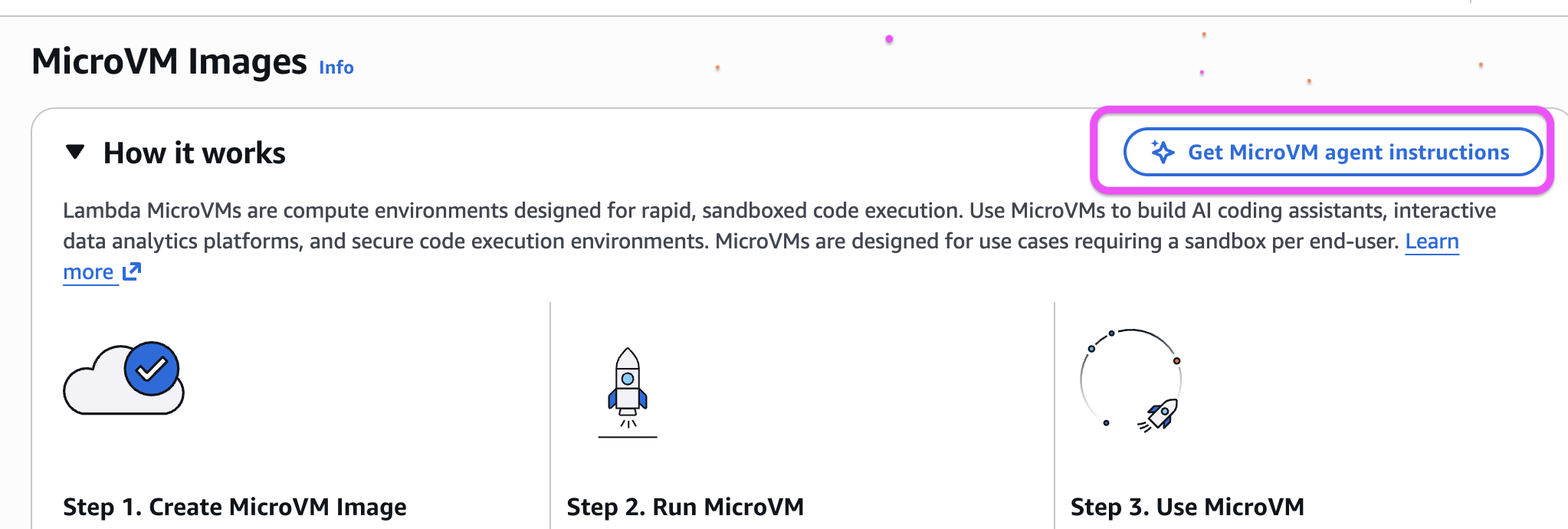
Figure 1: Access MicroVM agent instructions

Figure 1: Access MicroVM agent instructions

Next, copy the agent installation instructions and paste it in your terminal to begin developing.
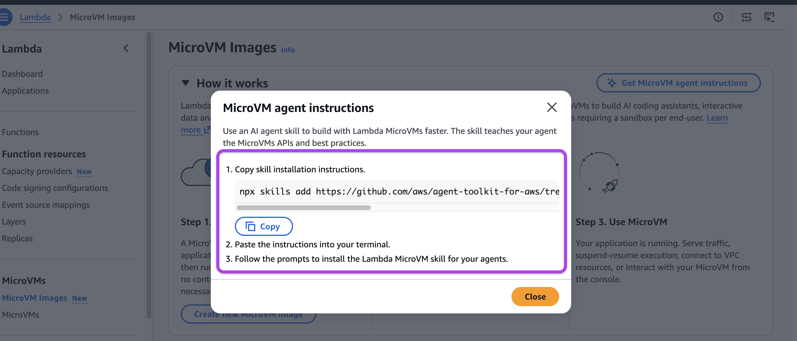
Figure 2: Copy agent instructions

Figure 2: Copy agent instructions

The following screenshot demonstrates the skill in action in an AI coding assistant. Using the skill, the coding assistant agent generates a detailed plan to build the analytics notebook solution, executes the plan, and validates correct execution.
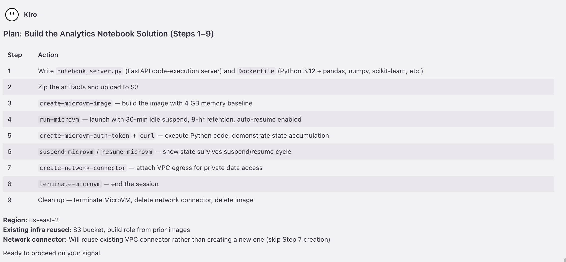
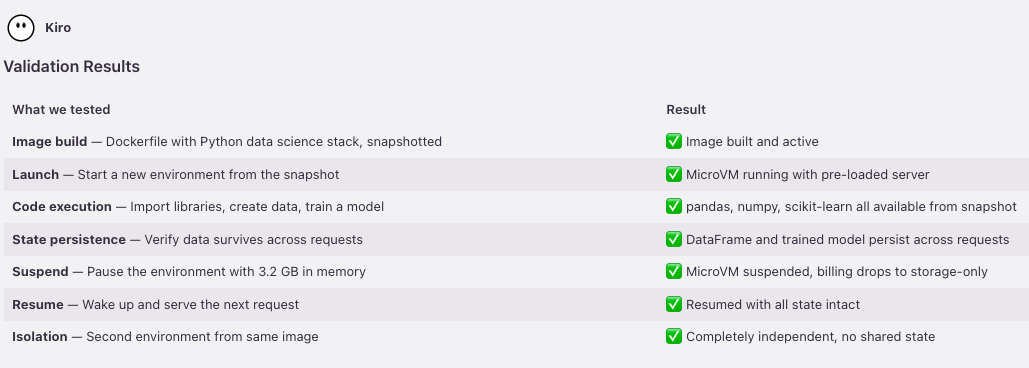
Figure 3: Agent-driven development with MicroVMs

Figure 3 continued: Agent-driven development with MicroVMs

Figure 3 continued: Agent-driven development with MicroVMs

Lambda MicroVMs as sandboxes for Claude Managed Agents

You can also use AWS Lambda MicroVMs as a managed sandbox provider for Claude Managed Agents self-hosted sandboxes. This pattern keeps the orchestration within your Anthropic environment, which hosts the agent loop and Claude model, but moves tool execution into AWS Lambda MicroVMs, so the agent’s code, filesystem, and network egress never leave the infrastructure you control. You control the execution environment – what is installed, what network access is available, and what resources the agent can reach. For integration details, refer to the Lambda MicroVMs developer guide.

Snapshot compatibility considerations

Lambda MicroVMs are started from snapshots of pre-initialized memory and disk state. This has a few implications for how you build applications:

Uniqueness: Content generated and retained within a MicroVM image is shared across all MicroVMs started from that image. To maintain uniqueness for content such as unique IDs, secrets, or random seeds, generate these values after each MicroVM is started. If your application code uses OpenSSL, use the AWS-provided base container image from public.ecr.aws/lambda/microvms:al2023-minimal to build your MicroVM image.

Ephemeral credentials and network connections: Credentials and connections established during MicroVM image creation – or before a MicroVM is suspended – may expire or terminate by the time the MicroVM starts or resumes. Design your application to refresh these credentials and re-establish connections on startup. AWS SDK clients re-establish connections automatically in most cases.

Lambda MicroVMs provides lifecycle hooks that are executed when a MicroVM is started or resumed. Use these hooks to restore uniqueness and to re-establish network connections or ephemeral credentials. For more details, refer to the Working with snapshots section in the Lambda MicroVMs developer guide.

Pricing

Lambda MicroVMs pricing comprises compute, snapshots, and data transfer (at standard AWS rates, including data transferred to your VPC). You have two cost management levers: baseline-plus-consumption billing and idle-suspension. With baseline-plus-consumption billing, your bill tracks closer to your actual resource usage rather than peak resource usage. You configure your MicroVM’s baseline resource allocation to match your workload’s average resource utilization – not peak. During peak activity, your MicroVM can vertically scale up to 4x of the configured baseline automatically and resource usage above the baseline is only billed during active use. You configure the baseline by setting memory, and CPU is allocated in a 2:1 memory-to-CPU ratio – the default is 2GB / 1vCPU, with a corresponding peak of 8 GB / 4 vCPU. Supported baseline and peak values are shown in Figure 4.
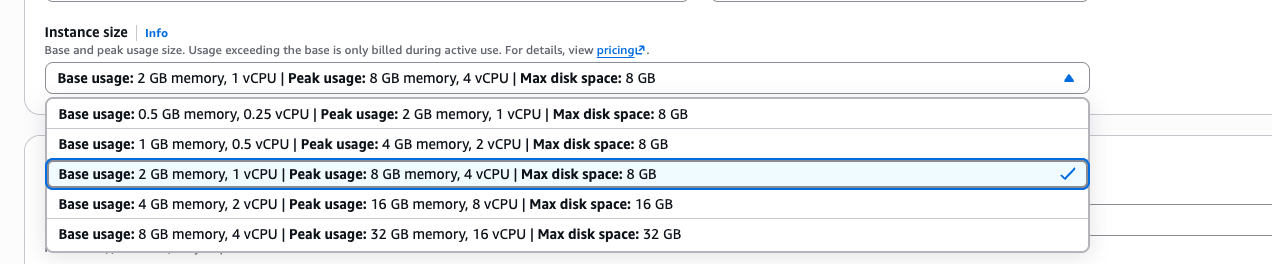
Figure 4: Baseline and peak resource configuration

Figure 4: Baseline and peak resource configuration

During extended idle periods, you can suspend your MicroVM to preserve memory and disk state at storage-only rates, resuming near-instantly when needed – no compute charges while suspended. For full pricing details, see AWS Lambda pricing.

Conclusion

Lambda MicroVMs extends the serverless compute model beyond invocation-based functions to long-running, stateful environments that execute code supplied by end users or AI. Development teams can focus on core application development while Lambda provides secure isolation and near-instant startup performance. Whether you’re building an AI coding assistant, an interactive development platform, an IT security platform, or a data analytics workload, the pattern is the same: define your environment in a Dockerfile, build a MicroVM Image once, launch isolated MicroVMs on demand, interact over HTTPS, and terminate when done.

To get started, visit the AWS Lambda MicroVMs developer guide or start building with the MicroVMs agent skill, available through the AWS Lambda console.
Deploying AI models for inference with AWS Lambda using zip packaging

Post Syndicated from Ayush Kulkarni original https://aws.amazon.com/blogs/compute/deploying-ai-models-for-inference-with-aws-lambda-using-zip-packaging/

AWS Lambda provides an event-driven programming model, scale-to-zero capability, and integrations with over 200 AWS services. This can make it a good fit for CPU-based inference applications that use customized, lightweight models and complete within 15 minutes.

Users usually package their function code as container images when using machine learning (ML) models that are larger than 250 MB, which is the Lambda deployment package size limit for zip files. In this post, we demonstrate an approach that downloads ML models directly from Amazon S3 into your function’s memory so that you can continue packaging your function code using zip files. To optimize startup latency without implementing application-level performance optimizations, we use Lambda SnapStart. SnapStart is an opt-in capability available for Java, Python, and .NET functions that optimizes startup latency—from 16.5s down to 1.6s for the application used in this post.

Application architecture

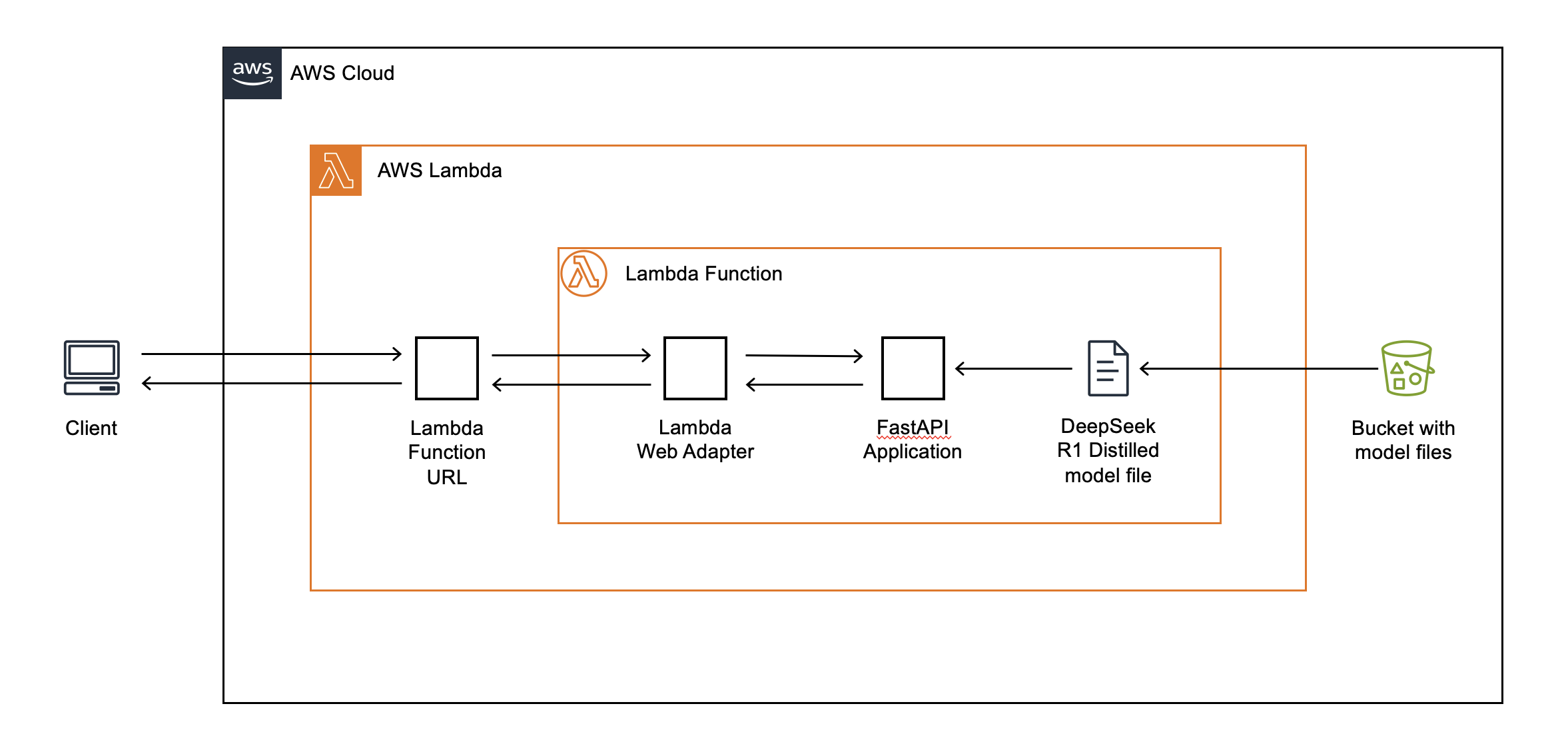
In this post, we demonstrate how to build a chatbot, using a 4-bit quantized version of the DeepSeek-R1-Distill-Qwen-1.5B-GGUF model for inference along with Lambda Function URL (FURL) and Lambda Web Adapter (LWA) to stream text responses. A FURL is a dedicated HTTP(s) endpoint for your Lambda function, and you can use LWA, an open-source project available on AWS Labs, for familiar web application frameworks (such as FastAPI, Next.JS, or Spring Boot) with Lambda. For a detailed explanation of how this response streaming architecture works, refer to this AWS Compute post.

Today, Lambda functions are run on CPU-based Amazon Elastic Compute Cloud (Amazon EC2) instances that use x86 and ARM64 architectures. For this reason, you must use SDKs that enable large language model (LLM) inference on CPUs. In this post, we also demonstrate how to use the llama.cpp project (through the llama-cpp-python library) and the FastAPI web framework to handle web requests. To use models that exceed the 250 MB zip package size limit of Lambda, you can download them from an S3 bucket during function initialization. The following figure describes this architecture in detail.

Architecture diagram demonstrating an AI inference workload with AWS Lambda FURLs and AWS Lambda Web Adapter

Figure 1: Application architecture

You can refer to this GitHub repository for the application code used in this example.

Downloading ML models during function initialization

As an alternative to packaging ML models using OCI container images, you can download them from durable storage, such as Amazon S3, during initialization. Initialization (or INIT) refers to the phase when Lambda downloads your function code, starts the language runtime and runs your function initialization code, which is code outside the handler. Loading large files directly into memory can be faster than first downloading them to disk and then loading them into memory. To do so, you can use a Linux capability called memfd, to directly download the ML model from Amazon S3 directly into memory, while referencing it using a standard file descriptor. Referencing the model using a file descriptor is necessary for llama.cpp to successfully import the model. This is comprised of two steps.

First, create a memory-only file descriptor:


    libc = ctypes.CDLL("libc.so.6", use_errno=True)
    MFD_CLOEXEC = 1
    
    memfd_create = libc.memfd_create
    memfd_create.argtypes = [ctypes.c_char_p, ctypes.c_uint]
    memfd_create.restype = ctypes.c_int
    
    fd = memfd_create(b"model", MFD_CLOEXEC)
    if fd == -1:
        errno = ctypes.get_errno()
    raise OSError(errno, f"memfd_create failed: {os.strerror(errno)}")
    
    return fd

Then, download the model into the memory-mapped file referenced by the previously created file descriptor.

def download_model_to_memfd(bucket, key, chunk_size=100*1024*1024):  # 100MB chunks

    s3 = boto3.client('s3')
    
    # Get file size
    response = s3.head_object(Bucket=bucket, Key=key)
    file_size = response['ContentLength']
    
    # Create memory file
    fd = create_memfd()
    
    # Pre-allocate the full file size
    try:
        os.ftruncate(fd, file_size)
    except OSError as e:
        logger.error(f"Failed to allocate {file_size/1024/1024:.2f}MB in memory: {e}")
        cleanup_fd(fd)
        raise RuntimeError(f"Not enough memory to load model of size {file_size/1024/1024:.2f}MB")
    
    # Calculate parts
    parts = []
    for start in range(0, file_size, chunk_size):
        end = min(start + chunk_size - 1, file_size - 1)
        parts.append({'start': start, 'end': end})
    
    logger.info(f"Downloading {file_size/1024/1024:.2f}MB in {len(parts)} parts")
    
    # Download parts concurrently
    download_func = partial(download_part, s3, bucket, key, fd)
    with ThreadPoolExecutor(max_workers=multiprocessing.cpu_count()) as executor:
        executor.map(download_func, parts)
    
    fd_path = f"/proc/self/fd/{fd}"
    return fd, fd_path

Querying the chatbot

After deploying our sample chatbot application, we begin interacting with it.

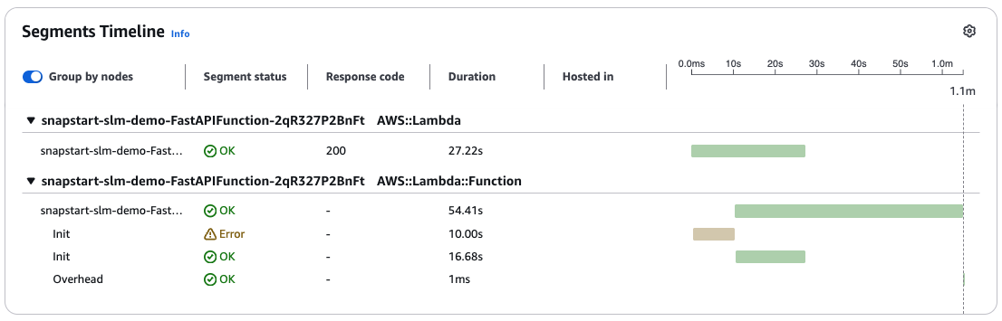
The first query to the chatbot results in a new execution environment being initialized. When Lambda runs the initialization code described in the previous section, your ML model is directly downloaded from Amazon S3 into the function’s memory. After this, Lambda runs the function’s handler method. Looking at the X-Ray trace segment in the following figure, we observe that the first Init times out after 10 s. The second Init completes in 16.68 s. Furthermore, the first Init times out because Lambda limits the duration of this phase to 10s. If Init takes longer than this, then Lambda retries it during function invocation applying the function’s configured execution duration timeout.

Screenshot of AWS X-Ray Segments demonstrating INIT duration of 16.68 s

Figure 2: Init duration, indicated by AWS X-Ray trace segment

Optimizing startup performance with SnapStart

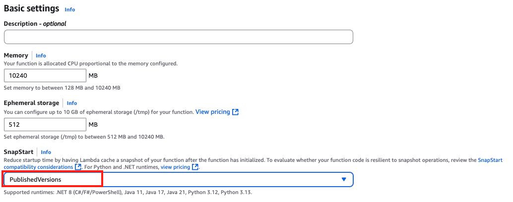
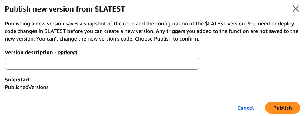
To optimize function startup latency, you can use Lambda SnapStart. SnapStart is designed to optimize startup latency stemming from long-running function initialization code. Lambda uses SnapStart to initialize your function when you publish a function version, as shown in the following figure. Then, Lambda takes a Firecracker microVM snapshot of the memory and disk state of the initialized execution environment, encrypts the snapshot, and intelligently caches it to optimize retrieval latency.

Screenshot of AWS Lambda Console showing how to enable SnapStart for your Lambda function

Figure 3: Enabling SnapStart

Querying the chatbot again shows a significant speed-up in initialization latency. You can verify this by viewing your function’s Amazon CloudWatch Logs, and searching for the “RESTORE_REPORT” log line, as shown in the following figure. For the sample application used, restore duration is 1.39 s. This is a considerable improvement over the Init duration of 16.68 s. Performance results may vary. But best of all, you don’t need to change a single line of code to achieve this improvement!

Screenshot of Amazon CloudWatch Logs demonstrating RESTORE duration of 1.39 s

Figure 4: Achieving faster startup latency with SnapStart

Tuning inference performance

Inference performance depends on the CPU resources allocated to your function. Lambda allocates CPU power in proportion to the amount of memory configured for your function. Allocating more memory results in faster inference results, measured by the rate at which prompt tokens are evaluated (tokens evaluated per second), and the rate at which output tokens are produced (tokens generated per second). For this example, we allocate the maximum—in other words 10 GB memory—to maximize performance. Performance results obtained at other memory size configurations are included in the following table. As the table shows, doubling the memory allocated from 5 GB to 10 GB results in an 83% improvement in tokens evaluated and generated (per second), with only a 24% increase in billed GB-seconds. Performance results may vary. Refer to the sample code to instrument performance at different memory sizes.

Memory
Size (MB)
Tokens evaluated per second

Tokens generated

per second

Billed Duration (ms)

Billed

GB-seconds

10240 44.68 29.53 36,660 366.60
9216 41.67 26.77 37,690 339.21
8192 37.17 22.05 44,298 354.38
7168 33.67 21.78 44,818 313.73
6144 28.89 18.43 52,579 315.47
5120 24.41 16.07 59,036 295.18
4096 19.07 12.94 72,648 290.59
3072 13.39 9.20 101,468 304.40
2048 10.01 6.77 135,862 271.72

Table 1: Inference performance at different memory sizes

Understanding how application costs scale with usage

To estimate the cost of running this workload, we begin by making some assumptions about our traffic patterns. We estimate about 30,000 inference calls per month to our Lambda function, with each inference call averaging 10s in duration. We set function memory to 10 GB, because it represents the ideal price-performance for our use case. We deploy our application in the US-West-2 (Oregon) AWS Region. Initially, because our number of invokes is low, we assume a 5% cold-start rate. In other words, 5% of invokes result in a cold-start when a new execution environment is created. When using SnapStart with the Lambda managed Python runtime, you are charged for caching your function’s snapshot and for restoring execution from your function’s snapshot.

With these parameters, the monthly Lambda bill is $91.1, calculated as shown in the following table. The monthly costs shown in the table are only illustrative.

Charge Calculation Monthly Cost
Compute 30,000 inferences * 10 seconds per inference * 10 GB (configured memory) * $0.00001667 per GB-second $50.01
Requests $0.2 per million requests * 30,000 inferences $0.006
SnapStart – Cache 10 GB function memory * 2.59M GB-seconds per month * $0.0000015046 per GB-second $38.99
SnapStart – Restore 10 GB function memory * $0.0001397998 per GB restore * 1500 cold-starts $2.09
Total Compute + Requests + SnapStart Cache + SnapStart Restore $91.1

At low invocation volume, the added charges for the SnapStart account for approximately 50% of total monthly cost. For this added charge, cold-start latency reduces from 16.68 s to1.39 s, without having to implement complex optimizations ourselves. We can demonstrate how these costs scale with usage. We assume that our chatbot grows in popularity with traffic increasing 10 times to 300,000 monthly inference calls. Although cold-start rates for individual Lambda functions can vary due to several factors, Lambda’s re-use of execution environments generally results in cold-start rates decreasing with higher traffic volume. For the purposes of this example, we assume that our cold-start rate drops to 1% of all invokes with the 10 times growth in traffic.With these assumptions, our monthly Lambda bill at 10 times higher traffic volume is $543.3. Added charges for SnapStart now constitute less than 10% of our total bill, as shown in the following table. Monthly costs shown in this table are only illustrative.

Charge Calculation Monthly Cost
Compute 300,000 inferences * 10 seconds per inference * 10 GB (configured memory) * $0.00001667 per GB-second $500.01
Requests $0.2 per million requests * 300,000 inferences $0.06
SnapStart – Cache 10 GB function memory * 2.59M GB-seconds per month * $0.0000015046 per GB-second $38.99
SnapStart – Restore 10 GB function memory * $0.0001397998 per GB restore * 3000 cold-starts $4.18
Total Compute + Requests + SnapStart Cache + SnapStart Restore $543.24

Considerations


Lambda functions are run on CPU-based EC2 instances. If your ML models need GPU-based inference, foundational LLMs, or exceed the Lambda limits on execution duration (15 minutes) and function memory (10 GB), then you can use AWS Machine Learning, AWS Generative AI, or AWS Compute services.

Moreover, you should know the following things about Lambda SnapStart:

Handling uniqueness: If your initialization code generates unique content that is included in the snapshot, then the content isn’t unique when it’s reused across execution environments. To maintain uniqueness when using SnapStart, you must generate unique content after initialization, such as if your code uses custom random number generation that doesn’t rely on built-in-libraries or caches any information such as DNS entries that might expire during initialization. To learn how to restore uniqueness, visit Handling uniqueness with Lambda SnapStart in the Lambda Developer Guide.

Performance tuning: To maximize performance, we recommend that you preload dependencies and initialize resources that contribute to startup latency in your initialization code instead of in the function handler. This moves the latency associated with these operations during version publish, rather than during function invocation and can yield faster startup performance. To learn more, visit Performance tuning for Lambda SnapStart in the Lambda Developer Guide.

Networking best practices: The state of connections that your function establishes during the initialization phase isn’t guaranteed when Lambda resumes your function from a snapshot. In most cases, network connections that an AWS SDK establishes automatically resume. For other connections, review the Networking best practices for Lambda SnapStart in the Lambda Developer Guide.

Conclusion

In this post, we demonstrated how you can download ML models directly from Amazon S3 into your function’s memory, enabling you to deploy your AWS Lambda functions using zip packages. To optimize startup latency without implementing application-level performance optimizations, we also demonstrated the use of Lambda SnapStart, an opt-in capability available for Java, Python, and .NET. For the application used in this post, SnapStart reduced startup latency from 16.68 s down to 1.39 s.

To learn more about Lambda, refer to our documentation. For details about Lambda SnapStart, refer to our launch posts for Java, Python and .Net, and the documentation.

You can refer to this GitHub repository for the application code used in this example.

Under the hood: how AWS Lambda SnapStart optimizes function startup latency

Post Syndicated from Ayush Kulkarni original https://aws.amazon.com/blogs/compute/under-the-hood-how-aws-lambda-snapstart-optimizes-function-startup-latency/

When building applications using AWS Lambda, optimizing function startup is an important step to improve performance for latency sensitive applications. The largest contributor to startup latency (often referred to as cold start time) is the time that Lambda spends initializing your function code. Lambda SnapStart is a feature available for Java, Python, and .NET runtimes that helps reduce variable cold start latency from several seconds (or higher) to as low as sub-second. SnapStart typically needs zero or minimal changes to your application code and makes it easier to build highly responsive and scalable applications without implementing complex performance optimizations. This post explains how SnapStart works under the hood and provides recommendations to improve application performance when using SnapStart.

If your function already initializes within hundreds of milliseconds, then AWS recommends using Lambda Provisioned Concurrency to achieve double-digit millisecond startup latency.

What is a cold-start?

Lambda runs your function code in an isolated, secure execution environment that uses Firecracker microVM technology. When you first invoke a Lambda function, Lambda creates a new execution environment for the function to run in. Lambda downloads your function code, starts the language runtime, and runs your function initialization code, which is code outside the handler. This initialization process (INIT) is called a cold start. Then, Lambda runs your function handler code to invoke the function. A Lambda execution environment only handles a single invoke request at a time. The following figure shows the lifecycle of a typical invocation request.

Figure 1. Function invocation lifecycle without SnapStart

Figure 1. Function invocation lifecycle without SnapStart

After the function finishes running, Lambda doesn’t stop the execution environment right away. When your function receives another invocation request, Lambda attempts to route the request to the idle but already running execution environment. As the INIT process has already run for this execution environment, this invoke is called a warm start. When more traffic arrives than Lambda has available idle execution environments, Lambda initializes new execution environments to serve the additional requests, performing the cold start initialization process again.

The last step of the cold start, initializing function code, typically takes the longest. This depends on the startup tasks that you execute in your code and the programming language runtime or framework you use. For languages such as Java and .NET, startup latency is impacted by just-in-time compilation of static code in loaded classes. For Python, it can be impacted if your executed code contains numerous or large modules. Other startup tasks, such as downloading machine learning (ML) models, can also take several seconds to complete, which adds to your function’s initialization latency. SnapStart is designed to optimize this last step of the cold start process and achieves this in three stages.

Stage 1: Snapshotting your Lambda function

When using SnapStart, the Lambda execution environment lifecycle changes. When you enable SnapStart for a particular function, publishing a new function version triggers the snapshotting process. The process runs the function initialization phase and takes an immutable, encrypted Firecracker microVM snapshot of the memory and disk state of the initialized execution environment, caching and chunking the snapshot for reuse. Code paths that are not executed during initialization, such as classes loaded on-demand through dependency injection, are not included in your function’s snapshot. To improve snapshot efficiency, proactively execute code paths during the initialization phase, or use runtime hooks to run code before Lambda creates a snapshot.

Snapshot creation can take a few minutes, during which your function version remains in the PENDING state, becoming ACTIVE when the snapshot is ready.

When you subsequently invoke your function, Lambda restores new execution environments from this snapshot. This optimization makes the invocation time faster and more predictable, because creating new a execution environment no longer requires an initialization.

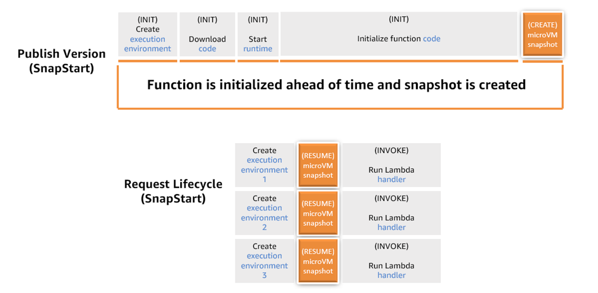
The following figure shows the lifecycle of a SnapStart configured function.

Diagram illustrating how AWS Lambda SnapStart works. The top section shows the 'Publish Version' phase, where the function is initialized ahead of time by creating the execution environment, downloading the code, starting the runtime, and initializing the function code. At the end of this phase, a microVM snapshot is created. The bottom section shows the 'Request Lifecycle' using SnapStart: each new execution environment resumes from the pre-initialized microVM snapshot and immediately invokes the Lambda handler. This allows multiple environments to start faster by skipping initialization steps.

Figure 2. Function invocation lifecycle with SnapStart

After Lambda creates a snapshot, it periodically regenerates it to apply security patches, runtime updates, and software upgrades. Your invocation requests continue to work throughout the regeneration process.

Stage 2: Storing snapshots for low-latency retrieval at Lambda scale

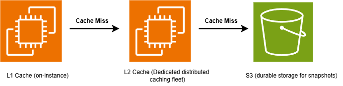
Lambda operates at a high scale, processing tens of trillions of invocation requests every month. To efficiently manage and retrieve snapshots at this volume of traffic, Lambda uses storage and caching components. These consist of three layers: Amazon S3 for durable storage, a dedicated distributed cache, and a local cache on Lambda worker nodes.

Lambda stores function snapshots in Amazon S3, dividing them into 512 KB chunks to optimize retrieval latency. Retrieval latency from Amazon S3 can take up to hundreds of milliseconds for each 512 KB chunk. Therefore, Lambda uses a two-layer cache to speed-up snapshot retrieval.

When you enable SnapStart, during the optimization process, Lambda stores snapshot chunks in a layer two (L2) cache. This layer is a dedicated distributed cache instance fleet purpose-built by Lambda. Lambda stores a separate copy of each snapshot per AWS Availability Zone (AZ). To balance performance with costs, Lambda may not proactively cache unused snapshot chunks, instead caching them after they are first accessed. Chunks remain cached in the L2 fleet as long as your function version is active. The snapshot restore performance from the L2 layer is typically single digit milliseconds for a 512 KB chunk.

Lambda also maintains a layer one (L1) cache located on Lambda worker nodes, the Amazon Elastic Compute Cloud (Amazon EC2) instances handling function invocations. This layer is available locally, thus it provides the fastest performance, typically 1 millisecond for a 512 KB chunk. Functions with more frequent invocations are more likely to have their snapshot chunks cached in this layer. Functions with fewer invocations are automatically evicted from this cache, because it is bound by the worker instance disk capacity. When a snapshot chunk is not available in the L1 cache, Lambda retrieves the chunk from the L2 cache layer.

Figure 3. SnapStart tiered cache

Figure 3. SnapStart tiered cache

Stage 3: Resuming execution from restored snapshots

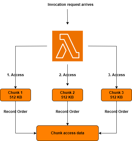
Resuming execution from snapshots with low latency is the final SnapStart stage. This involves loading the retrieved snapshot chunks into your function execution environment. Typically, only a subset of the retrieved snapshot is needed to serve an invocation. Storing snapshots as chunks lets Lambda optimize the resume process by proactively loading only the necessary subset of chunks. To achieve this, Lambda tracks and records the snapshot chunks that the function accesses during each function invocation, as shown in the following figure.

Figure 4. Initial invocation, record chunk access pattern

Figure 4. Initial invocation, record chunk access pattern

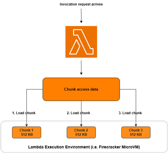
After the first function invocation, Lambda refers to this recorded chunk access data for subsequent invokes, as shown in the following figure. Lambda proactively retrieves and loads this “working set” of chunks before they are needed for execution. This significantly speeds up cold-start latency. If every invoke executes the same code path, then all necessary chunks are tracked after the first invoke. If your Lambda function includes a method that is conditionally invoked once every five cold starts, then Lambda adds the corresponding chunks representing this method to the chunk access metadata after five cold starts.

Figure 5. Subsequent invocation, load chunks in order of access

Figure 5. Subsequent invocation, load chunks in order of access

Understanding SnapStart function performance

The speed of restoring a snapshot depends on its contents, size, and the caching tier used. As a result, SnapStart performance can vary across individual functions.

Function performance improves with more invocations

Frequently invoked functions are more likely to have their snapshots cached in the L1 layer, which provides the fastest retrieval latency. Infrequently accessed portions of snapshots for functions with sporadic invokes are less likely to be present in the L1 layer, resulting in slower retrieval latency from the L2 and S3 cache layers. Chunk access data for functions with more invocations is also more likely to be “complete”, which speeds up snapshot restore latency.

Pre-load code paths to optimize snapshot restore latency

To maximize the benefits of SnapStart, preload dependencies, initialize resources, and perform heavy computation tasks that contribute to startup latency in your initialization code instead of in the function handler. Code paths not executed during your function’s INIT phase, such as application classes loaded on-demand through dependency injection, are not included in your function’s snapshot. You can further improve SnapStart effectiveness by proactively executing these code paths during function initialization. You can also run code using runtime hooks and invoking your handler during the initialization phase before creating the snapshot. To achieve this, refer to the documentation and posts for Spring Boot and .NET applications to implement the performance tuning.

Performance differs depending on function size

SnapStart performance depends on how quickly Lambda can retrieve and load cached snapshots into your function execution environment. Larger function sizes increase the size of snapshots, and thus the number of chunks, which causes performance to differ for functions of varying sizes.

Not all functions benefit from SnapStart

SnapStart is designed to improve startup latency when function initialization takes several seconds, due to language-specific factors or because of initializing and loading software dependencies and frameworks. If your functions initialize within hundreds of milliseconds, you are unlikely to experience a significant performance improvement with SnapStart. For these scenarios, we recommend Provisioned Concurrency, which pre-initializes execution environments, delivering double-digit millisecond latency.

Conclusion

AWS Lambda SnapStart can deliver as low as sub-second startup performance for Java, .NET, and Python functions with long initialization times. This post explores how the Lambda lifecycle changes with SnapStart and how Lambda efficiently stores and loads snapshots to improve start up performance. SnapStart helps developers build highly responsive and scalable applications without provisioning resources or implementing complex performance optimizations.

To learn more about SnapStart, refer to the documentation and launch posts for Java, and Python and .NET. For performance tuning, refer to the SnapStart best practices section for your preferred language runtime. This post outlines approaches to pre-load code paths to further optimize startup latency. Find more information and sample applications built using SnapStart on Serverlessland.com.