Post Syndicated from Erik Anderson original https://aws.amazon.com/blogs/big-data/scale-amazon-redshift-to-meet-high-throughput-query-requirements/
Many enterprise customers have demanding query throughput requirements for their data warehouses. Some may be able to address these requirements through horizontally or vertically scaling a single cluster. Others may have a short duration where they need extra capacity to handle peaks that can be addressed through Amazon Redshift concurrency scaling. However, enterprises with consistently high demand that can’t be serviced by a single cluster need another option. These enterprise customers require large datasets to be returned from queries at a high frequency. These scenarios are also often paired with legacy business intelligence (BI) tools where data is further analyzed.
Amazon Redshift is a fast, fully managed cloud data warehouse. Tens of thousands of customers use Amazon Redshift as their analytics platform. These customers range from small startups to some of the world’s largest enterprises. Users such as data analysts, database developers, and data scientists use Amazon Redshift to analyze their data to make better business decisions.
This post provides an overview of the available scaling options for Amazon Redshift and also shares a new design pattern that enables query processing in scenarios where having multiple leader nodes are required to extract large datasets for clients or BI tools without introducing additional overhead.
Common Amazon Redshift scaling patterns
Because Amazon Redshift is a managed cloud data warehouse, you only pay for what you use, so sizing your cluster appropriately is critical for getting the best performance at the lowest cost. This process begins with choosing the appropriate instance family for your Amazon Redshift nodes. For new workloads that are planning to scale, we recommend starting with our RA3 nodes, which allow you to independently tailor your storage and compute requirements. The RA3 nodes provide three instance types to build your cluster with: ra3.xlplus, ra3.4xlarge, and ra3.16xlarge.
Horizontal cluster scaling
Let’s assume for this example, you build your cluster with four ra3.4xlarge nodes. This configuration provides 48 vCPUs and 384 GiB RAM. Your workload is consistent throughout the day, with few peaks and valleys. As adoption increases and more users need access to the data, you can add nodes of the same node type to your cluster to increase the amount of compute power available to handle those queries. An elastic resize is the fastest way to horizontally scale your cluster to add nodes as a consistent load increases.
Vertical cluster scaling
Horizontal scaling has its limits, however. Each node type has a limit to the number of nodes that can be managed in a single cluster. To continue with the previous example, ra3.4xlarge nodes have a maximum of 64 nodes per cluster. If your workload continues to grow and you’re approaching this limit, you may decide to vertically scale your cluster. Vertically scaling increases the resources given to each node. Based on the additional resources provided by the larger nodes, you will likely decrease the quantity of nodes at the same time.
Rather than running a cluster with 64 ra3.4xlarge nodes, you could elastically resize your cluster to use 16 ra3.16xlarge nodes and have the equivalent resources to host your cluster. The transition to a larger node type allows you to horizontally scale with those larger nodes. You can create an Amazon Redshift cluster with up to 16 nodes. However, after creation, you can resize your cluster to contain up to 32 ra3.xlplus nodes, up to 64 ra3.4xlarge nodes, or up to 128 ra3.16xlarge nodes.
Concurrency scaling
In March 2019, AWS announced the availability of Amazon Redshift concurrency scaling. Concurrency scaling allows you to add more query processing power to your cluster, but only when you need it. Rather than a consistent volume of workload throughout the day, perhaps there are short periods of time when you need more resources. When you choose concurrency scaling, Amazon Redshift automatically and transparently adds more processing power for just those times when you need it. This is a cost-effective, low-touch option for burst workloads. You only pay for what you use on a per-second basis, and you accumulate 1 hour’s worth of concurrency scaling credits every 24 hours. Those free credits have met the needs of 97% of our Amazon Redshift customers’ concurrency scaling requirements, meaning that most customers get the benefits of concurrency scaling without increasing their costs.
The size of your concurrency scaling cluster is directly proportional to your cluster size, so it also scales as your cluster does. By right-sizing your base cluster and using concurrency scaling, you can address the vast majority of performance requirements.
Multi-cluster scaling
Although the previous three scaling options work together to address the needs of the vast majority of our customers, some customers need another option. These use cases require large datasets to be returned from queries at a high frequency and perform further analysis on them using legacy BI tools.
While working with customers to address these use cases, we have found that in these scenarios, multiple medium-sized clusters can perform better than a single large cluster. This phenomenon mostly relates to the single Amazon Redshift leader node’s throughput capacity.
This last scaling pattern uses multiple Amazon Redshift clusters, which allows you to achieve near-limitless read scalability. Rather than relying on a single cluster, a single leader node, and concurrency scaling, this architecture allows you to add as many resources as needed to address your high throughput query requirements. This pattern relies on Amazon Redshift data sharing abilities to enable a seamless multi-cluster experience.
The remainder of this post covers the details of this architecture.
Solution overview
The following diagram outlines a multi-cluster architecture.
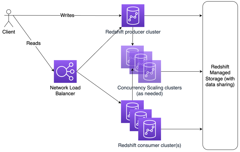
The first supporting component for this architecture is Amazon Redshift managed storage. Managed storage is available for RA3 nodes and allows the complete decoupling of compute and storage resources. This decoupling supports another feature that was announced at AWS re:Invent 2020—data sharing. Data sharing is primarily intended to let you share data amongst different data warehouse groups so that you can retain a single set of data to remove duplication. Data sharing ensures that the users accessing the data are using compute on their clusters rather than using compute on the owning cluster, which better aligns cost to usage.
In this post, we introduce another use case of data sharing: horizontal cluster scaling. This architecture allows you to create two or more clusters to handle high throughput query requirements while maintaining a single data source.
An important component in this design is the Network Load Balancer (NLB). The NLB serves as a single access point for clients to connect to the backend data warehouse for performing reads. It also allows changing the number of underlying clusters transparently to users. If you decide to add or remove clusters, all you need to do is add or remove targets in your NLB. It’s also important to note that this design can use any of the previous three scaling options (horizontal, vertical, and concurrency scaling) to fine-tune the number of resources available to service your particular workload.
Prerequisites
Let’s start by creating two Amazon Redshift clusters of RA3 instance type, and name them producer_cluster and consumer_cluster. For instructions, refer to Create a cluster.
In this post, our producer cluster is a central ETL cluster hosting enterprise sales data using a 3 TB Cloud DW dataset based on the TPC-DS benchmark.
The next step is to configure data sharing between the producer and consumer clusters.
Set up data sharing at the producer cluster
In this step, you need a cluster namespace from the consumer_cluster. One way to find the namespace value of a cluster is to run the SQL statement SELECT CURRENT_NAMESPACE when connected to the consumer_cluster. Another way is through the Amazon Redshift console. Navigate to your Amazon Redshift consumer_cluster, and find the cluster namespace located in the General information section.
After you connect to the producer cluster, create the data share and add the schema and tables to the data share. Then, grant usage to the consumer namespace by providing the namespace value. See the following code:
You can validate that data sharing was correctly configured by querying these views from the producer cluster:
Set up data sharing at the consumer cluster
Get the cluster namespace of the producer cluster by following same steps for the consumer cluster. After you connect to the consumer cluster, you can create a database referencing the data share of the producer cluster. Then you create an external schema and set the search path in the consumer cluster, which allows schema-level access control within the consumer cluster and uses a two-part notation when referencing shared data objects. Finally, you grant usage on the database to a user, and run a query to check if objects as part of data share are accessible. See the following code:
Set up the Network Load Balancer
After you set up data sharing at both the producer_cluster and consumer_cluster, the next step is to configure a Network Load Balancer to accept connections through a single endpoint and forward the connections to both clusters for reading data via queries.
As a prerequisite, collect the following information from the Amazon Redshift producer and consumer clusters on the Amazon Redshift console in the cluster properties section. Use the producer cluster information if consumer cluster is not mentioned below.
| Parameter Name | Parameter Description |
| VPCid | Amazon Redshift cluster VPC |
| NLBSubnetid | Subnet where the NLB ENI is created. The NLB and Amazon Redshift subnet need to be in the same Availability Zone. |
| NLBSubnetCIDR | Used for allowlisting inbound access in the Amazon Redshift security group |
| NLBPort | Port to be used by NLB Listener, usually the same port as Amazon Redshift port 5439 |
| RedshiftPrivateIP | IP address of Amazon Redshift leader node of the producer cluster |
| RedshiftPrivateIP | IP address of Amazon Redshift leader node of the consumer cluster |
| RedshiftPort: | Port used by Amazon Redshift clusters, usually 5439 |
| RedshiftSecurityGroup | Security group to allow connectivity to Amazon Redshift cluster |
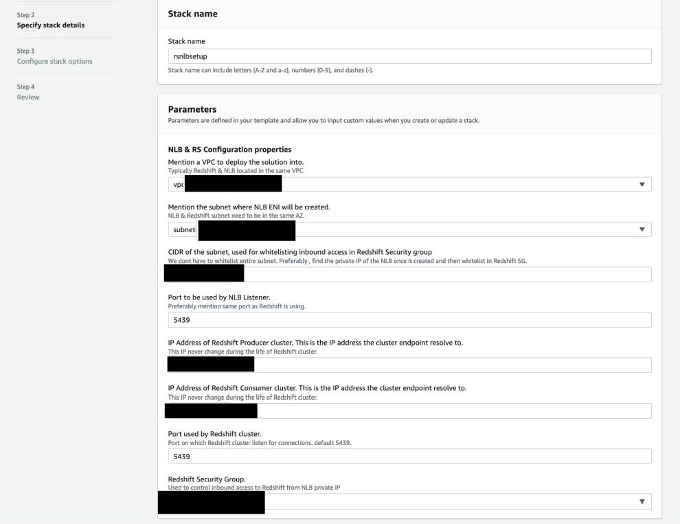
After you collect this information, run the AWS CloudFormation script NLB.yaml to set up the Network Load Balancer for the producer and consumer clusters. The following screenshot shows the stack parameters.
After you create the CloudFormation stack, note the NLB endpoint on the stack’s Outputs tab. You use this endpoint to connect to the Amazon Redshift clusters.
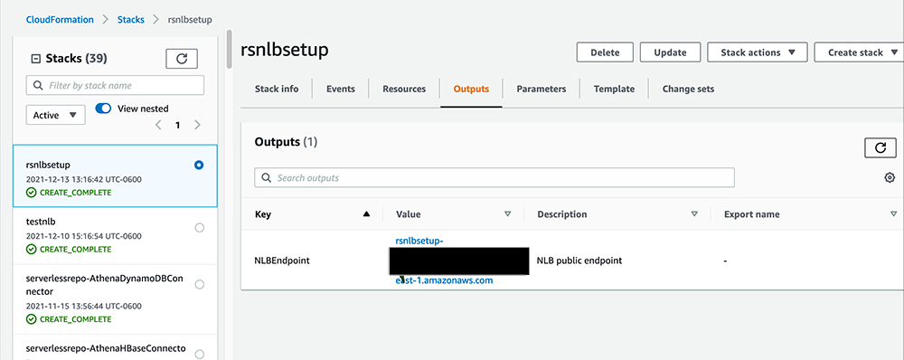
This NLB setup is done for the both producer and consumer clusters by the CloudFormation stack. If needed, you can add additional Amazon Redshift clusters to an existing NLB by navigating to Target groups page of the Amazon EC2 console. Then navigate to rsnlbsetup-target and add the Amazon Redshift cluster leader node private IP and port.
Validate the connections to the Amazon Redshift clusters
After you set up the NLB, the next step is to validate the connectivity to the Amazon Redshift clusters. You can do this by first configuring SQL tools like SQL Workbench, DBeaver, or Aginity Workbench and setting the host name and endpoint to the Amazon Redshift cluster’s NLB endpoint, as shown in the following screenshot. For additional configuration information, see Connecting to an Amazon Redshift cluster using SQL client tools.

Repeat this process a few times to validate that there are connections to both clusters. Similarly, you can use the same NLB endpoint as the host name while configuring.
As a next step, we use JMeter to show how the NLB is connecting to each of the clusters. The Apache JMeter application is open-source software, a 100% pure Java application designed to load test functional behavior and measure performance. Our NLB connects to each cluster in a round-robin manner, which enables even distribution of read load on Amazon Redshift clusters.
Setting up JMeter is out of scope of this post; refer to Building high-quality benchmark tests for Amazon Redshift using Apache JMeter to learn more about setting up JMeter and performance testing on an Amazon Redshift cluster.
The following screenshot shows the HTML output of the response data from JMeter testing. It shows that requests go to both the Amazon Redshift producer and consumer clusters in a round-robin manner.
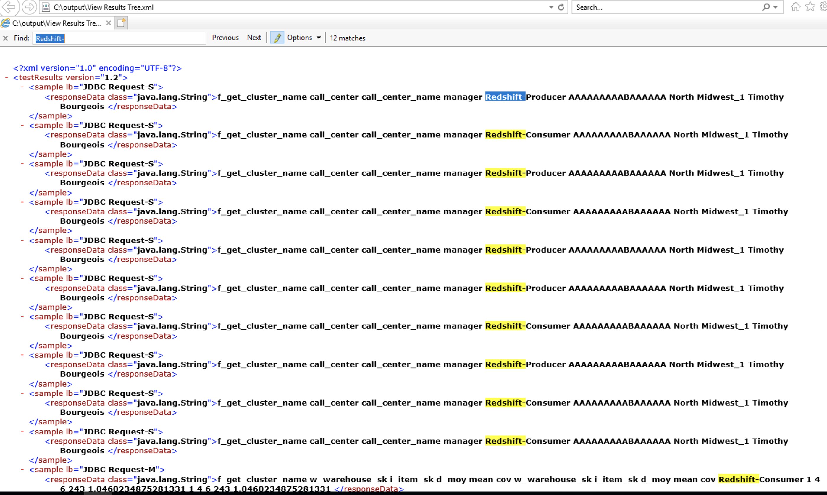
The preceding screenshot shows a sample output from running 20 SQL queries. Testing with over 1,000 SQL runs was performed with over four Amazon Redshift clusters, and the NLB was able to distribute them as evenly as possible across all of those clusters.
With this setup, you have the flexibility to add Amazon Redshift clusters to your NLB as needed and can configure data sharing to enable horizontal scaling of Amazon Redshift clusters. When demand reduces, you can either de-register some of the Amazon Redshift clusters at the NLB configuration or simply pause the Amazon Redshift cluster and the NLB automatically connects to only those clusters that are available at the time.
Conclusion
In this post, you learned about the different ways that Amazon Redshift can scale to meet your needs as they adjust over time. Use horizontal scaling to increase the number of nodes in your cluster. Use vertical scaling to increase the size of each node. Use concurrency scaling to dynamically address peak workloads. Use multiple clusters with data sharing behind an NLB to provide near-endless scalability. You can use these architectures independently or in combination with each other to build your high-performing, cost-effective data warehouse using Amazon Redshift.
To learn more about some of the foundational features used in the architecture mentioned in this post, refer to:
- Sharing Amazon Redshift data securely across Amazon Redshift clusters for workload isolation
- Amazon Redshift Update – Next-Generation Compute Instances and Managed, Analytics-Optimized Storage
- New – Concurrency Scaling for Amazon Redshift – Peak Performance at All Times.
About the Authors
 Erik Anderson is a Principal Solutions Architect at AWS. He has nearly two decades of experience guiding numerous Fortune 100 companies along their technology journeys. He is passionate about helping enterprises build scalable, performant, and cost-effective solutions in the cloud. In his spare time, he loves spending time with his family, home improvement projects, and playing sports.
 Rohit Bansal is a Analytics Specialist Solutions Architect at AWS. He specializes in Amazon Redshift and works with customers to build next-generation Analytics solutions using other AWS Analytics Services.