All posts by Jason Hunter

Bulk Executor for Amazon DynamoDB, Part 2: Lessons we learned the hard way

Post Syndicated from Jason Hunter original https://aws.amazon.com/blogs/architecture/bulk-executor-for-amazon-dynamodb-part-2-lessons-we-learned-the-hard-way/

In the Introducing open source Bulk Executor for Amazon DynamoDB blog post, you learned about the purpose and usage of the Bulk Executor tool. In this Part 2 post, we share the story of how we built it: the design tradeoffs, surprises, gotchas, and eventual workarounds. Think of it as your travel guide for working with Amazon DynamoDB and AWS Glue.

Design requirements

Bulk Executor is a project designed to run actions in bulk against many or all items in a table. For example you can mass delete old items or compare two tables for equality.

Three core requirements shaped most of the decisions that follow: running a bulk command should feel like a local script (real-time output, interruptible with ^C), it should scale to hundreds of parallel workers without the user managing infrastructure, and it should be straightforward to add new commands without tight coupling to the framework.

Selecting AWS Glue

We selected AWS Glue to drive the parallel execution. It’s a serverless service where you submit jobs that get distributed across workers (compute instances), each running tasks in parallel. For more information, see Key topics in Apache Spark. Our command-line client starts a job and AWS Glue handles distributing the work across potentially hundreds of workers.

We also considered Amazon Simple Queue Service (Amazon SQS) with AWS Lambda, AWS Fargate, Amazon EMR, and Ray. We decided to use AWS Glue because it gave us both serverless parallelism and a built-in DynamoDB connector, so we got much of the hard stuff at no cost. The following short code sample shows how to read or write items:

# Read from DynamoDB into a Spark DataFrame
dataframe = (
    spark.read
    .format("dynamodb")
    .option("dynamodb.input.tableName", "source")
    .option("dynamodb.throughput.read", "40000")
    .option("dynamodb.consistentRead", "false")
    .load()
)

# Write to DynamoDB from a Spark DataFrame
(
    dataframe.write
    .format("dynamodb")
    .option("dynamodb.output.tableName", "sink")
    .option("dynamodb.throughput.write", "40000")
    .option("dynamodb.item.size.check.enabled", "true")
    .save()
)

The Spark DataFrame gave us the built-in capabilities that we needed. Specifically:

  • A where/filter that accepts a Spark SQL condition to filter the data.
  • An orderBy that sorts the data.
  • A limit that controls the number of items.

On the back of these capabilities, we built the find command as our first command with its --where, --orderby, and --limit parameters requiring almost no coding on our part. If you want to print the 100 most recent undelivered orders, you can issue a bulk command like this:

./bulk find --table orders --where "status = 'undelivered'" --orderby timestamp desc --limit 100

The count command uses the same code but counts the items instead of printing them. The delete command does the same, but after finding the items runs parallel batch delete calls to remove them.

One downside of the Spark connector is that it doesn’t fully represent the source table data types. It simplifies the data and, for example, makes no distinction between a string set and a list of strings.

Estimating costs

When working against large tables, we wanted to give a cost estimate before starting the work. Predicting the future is always hard. Here’s how we did it.

For reads, we look at the table’s metadata (updated approximately every 6 hours, so beware a table that you recently loaded can read as smaller than it really is) to learn its recent size and calculate the read request units necessary for a full scan. For on-demand tables the math is straightforward: call the Pricing API to get the cost per million read request units for the region, multiply, done.

For provisioned mode, cost depends on the provisioned level, auto scaling headroom, and job duration, making estimation harder. Our heuristic is to take two-thirds of the on-demand price (divide by 1.5). The reasoning: a table provisioned at 100 percent utilization costs about 30 percent of the equivalent on-demand throughput. However, 100 percent is rarely achievable in practice. At 50 percent utilization, the cost is about 60 percent. We use 67 percent because it’s better to quote a little high.

For the delete command, write costs depend on how many items match, which we don’t know until after scanning. So delete calculates pricing in two phases: first the read cost estimate up front, then after finding the matches, the write cost based on the size of the deletion set.

For the fill command, which mass loads synthetic data according to a custom generator, we first generate some sample items to know the approximate size of the items, then price accordingly.

We don’t estimate AWS Glue Data Processing Unit (DPU) costs for two reasons. First, knowing how much compute will be required can’t be done simply. Second, we observed that for large jobs, DPU costs tend to be a small fraction of the DynamoDB costs. This makes sense, because an AWS Glue worker running at a small hourly cost can drive a huge amount of database activity. For small jobs, DPU is a larger fraction because of the overhead of getting things started, but the absolute dollars are low. You can specify --XWaitForDPU to see actual DPU costs reported after execution.

Every --X parameter is a parameter to the Bulk Executor itself, as opposed to the command being run. We modeled this after the Java Virtual Machine convention.

Job termination (^C)

We needed a way for the caller to terminate processing, for example if the pricing estimate comes back higher than expected. Pressing ^C stops the client Python script immediately but leaves the AWS Glue job running until its timeout.

We solved this by having the Python code catch the interrupt signal programmatically. An interrupt handler sees the ^C and sets an interrupted flag. This flag gets noticed by a watcher loop that’s always running. Usually it’s watching for things like AWS Glue state changes. But when it sees the interrupt, it actively directs the AWS Glue job to stop before proceeding with a clean exit of the client-side program. Now one ^C cleanly stops both sides.

Mandating point-in-time recovery (PITR)

A command like delete has the potential to delete more than anticipated. We made the design choice to require point-in-time recovery (PITR) to be enabled on any table receiving a mutating command. That way if your --where clause doesn’t do exactly what you wanted, you have a way to roll back.

This is one reason we built out the revert-export command to undo writes in place based on a PITR-driven incremental export. See our previous blog post “Recover from accidental DynamoDB changes using Bulk Executor”.

Watching execution (CloudWatch Live Tail)

In our first version, the client polled Amazon CloudWatch Logs for AWS Glue worker output. This was inefficient and meant output appeared delayed and in chunks. Switching to Amazon CloudWatch Live Tail let job output stream to the client in near real-time.

This introduced a problem: when find returned only a small number of matches things worked fine, but with large result sets we got incomplete output. The root cause: Live Tail displays at most 500 events per second. Beyond that, it streams only a sample of matching events.

Our solution was to write large output (from find or diff) to an Amazon Simple Storage Service (Amazon S3) bucket and only stream the first 10 results to the terminal, plus a link to the full data set.

Live Tail had two more surprises. Events can arrive out of order, so we built a reordering layer. Also, AWS Glue jobs can complete before their final log events appear in CloudWatch (there are a few seconds of propagation delay), so we couldn’t stop listening the moment the job stopped. We implemented a “microwave popcorn monitor”: stop listening only after a few seconds of silence.

Fast and useful error handling

When an AWS Glue task hits an error, it logs an exception and by default the stack trace goes into the logs for the client to see. If the error is in only one task, that’s manageable, if a bit verbose. But if it’s something that hits every task (like a bad --where clause), you get hundreds of identical stack traces flooding the terminal. We addressed this with four patterns.

On the client side, each command validates parameters before starting the AWS Glue job. A typo gets caught locally without AWS Glue ever spinning up.

Inside AWS Glue, we create an error_accumulator that’s a Spark accumulator. Instead of letting exceptions propagate up from tasks en masse, each task adds its exception to the accumulator. The Spark driver then extracts the first error and prints only that: one clean message instead of hundreds of duplicates, followed by a graceful job shutdown.

Continuously, on the client side, the Live Tail stream of events goes through a pattern matcher looking for error patterns that will never self-resolve (like AccessDeniedException, ModuleNotFoundError, OutOfMemoryError) and can trigger an immediate job stop rather than letting every task fail with the same error.

Also, to prevent “scary” stack traces for something as simple as a typo in a --where clause, we use a special app-specific exception type that a command can choose to throw when wanting to give an error and not a stack trace. Only developer-type errors should generate stack traces.

It took a while but we developed an approach to error handling that we liked: catch errors as quickly as possible, simplify them down to show the user only what’s necessary, and have the final line of each execution indicate if the job succeeded or failed (and why). We also added color coding (red for errors, yellow for warnings) to make issues easier to spot.

DynamoDB connector compared to direct access

The AWS Glue connector reads and writes DataFrames, but it has no way to delete items. For the delete command we had no choice but to make direct DynamoDB API calls. The command logic uses the connector to first find the matching items (giving a DataFrame), then iterates over the items to perform deletes using batch writes. Here’s a simplified version:

def delete_partition(partition, table_name, keys):
    table = dynamodb_resource.Table(table_name)
    with table.batch_writer() as batch:
        for record in partition:
            item = json.loads(record)
            key = {k: item[k] for k in keys}
            batch.delete_item(Key=key)

# Distribute deletes across workers
records.toJSON().foreachPartition(
    lambda partition: delete_partition(partition, table_name, keys)
)

Each Spark partition gets a slice of the matching items, and foreachPartition() runs the delete function in parallel across workers. The batch_writer() handles batching the individual deletes into efficient batch_write_item calls under the hood.

We built fill and load-export to write items directly by using batch_writer also, instead of constructing a DataFrame.

This pattern of going direct worked so well that it inspired us to rethink how we approached the first commands we wrote. We built a scancount command to explore whether counting could be faster without the connector.

The answer: consistently faster, because of less overhead. The connector-based count has to load every item into the AWS Glue context to then filter them and count what survived the filter. With scancount, we use DynamoDB segmented scan with push-down predicates and Select: COUNT so nothing comes out of the database except the count itself with the filter already having been applied. Each worker scans its own segment of the table in parallel:

def _count(table_name, index_name, filter_expression,
             segment, total_segments, total_matched_accumulator, error_accumulator):
    table = dynamodb_resource.Table(table_name)

    scan_kwargs = {
        "Select": "COUNT",
        "Segment": segment,
        "TotalSegments": total_segments
    }
    if index_name:
        scan_kwargs["IndexName"] = index_name
    if filter_expression:
        scan_kwargs["FilterExpression"] = filter_expression

    # Error handling code removed
    local_count = 0
    while True:
        response = table.scan(**scan_kwargs)
        local_count += response.get("Count", 0)
        if "LastEvaluatedKey" not in response:
            break
        scan_kwargs["ExclusiveStartKey"] = response["LastEvaluatedKey"]

    total_matched_accumulator.add(local_count)
    return local_count

parallelize_count = 100
rdd = spark_context.parallelize(range(parallelize_count), parallelize_count)
rdd.foreach(lambda worker_id: _count(table_name, index_name,
    filter_expression, worker_id, parallelize_count,
    total_matched_accumulator, error_accumulator))

The tradeoff: scancount accepts a raw --filter-expression instead of the higher-level --where Spark SQL syntax, since there’s no DataFrame involved.

The code for diff and copy also does direct reads instead of using the connector. With these commands, it wasn’t for speed but to make sure they keep perfect data type fidelity.

A side note on diff: it was important for each task to write its subset of output directly to its own Amazon S3 object, without ever centralizing the output back to the driver, which would not scale.

Rate limiting

The connector provides built-in rate limiting. However, for our commands making direct API calls (such as delete, fill, copy, and scancount), there’s no rate limiting. With enough AWS Glue workers running loops unconstrained, it usually generates unwanted throttles.

We built a distributed rate limiter that coordinates across all workers. The approach is described in detail in Rate-limiting calls to Amazon DynamoDB using Python Boto3, Part 1 and Part 2: Distributed Coordination.

Users control this with --XMaxReadRate and --XMaxWriteRate parameters. If unspecified, we investigate the environment to infer the appropriate rates based on account and table settings and quotas.

Recently, we added a feature to issue a (yellow) warning if the max read or write rate won’t allow the work to complete within the --XTimeout (which defaults to one hour). Better to warn the user early: if even the maximum rate can’t finish within the timeout, the user can restart with a higher rate or a longer timeout.

Building a library of commands

We started with the idea that commands should be straightforward to drop in, like new Unix commands. The loose coupling has paid off in contributions from outside the original core team. So far we’ve seen:

  • The diff command contributed by Chris Gillespie.
  • The sql command contributed by John Terhune.
  • The load command contributed by Arjan Schaaf.
  • The load-export and revert-export commands contributed by Ruskin Dantra.

Each command is its own Python module loaded by name. The contract is lightweight: export a run(job, spark_context, glue_context, parsed_args) function and use the shared conventions (the error_accumulator for exceptions, the distributed rate limiter for DynamoDB calls, and a shared library to help with cost estimates).

Upgrading to new AWS Glue versions, with the help of AI

A few months ago, we migrated from AWS Glue 4 to AWS Glue 5. The benefits: faster job startup and a new DynamoDB connector that loads directly into a DataFrame (the old connector required a DynamicFrame intermediate step, adding overhead and complexity).

The migration also gave us a chance to measure the new connector against the old one. We used AI tooling to generate a suite of stress tests comparing both connectors under AWS Glue 5, varying table sizes and read/write patterns. The AI ran these tests for hours, collected the results, and produced a comparison report that gave us the confidence the upgrade was worthwhile.

This migration had been on our backlog for a while and we kept postponing it. With AI handling the test generation and execution, we finished it in one interactive working session.

Since then we’ve upgraded to AWS Glue 6, this time to capture the 30 percent lower costs for DPU-hours.

Implementing an AI linter

We noticed some things are hard to test using either unit tests or end-to-end tests. For example, we have some data that exists in three places in three different formats, and we want to make sure those three definitions do not drift apart.

First, we have a README that explains some aspects of security. You can either let us generate a new AWS Glue job role for you, or you can pass in your own custom role by name. It explains, in English prose, the minimum AWS Identity and Access Management (IAM) permissions required by the AWS Glue job role if you create your own. That’s one definition.

The second definition is that when we create the role, we attach the right set of permissions on the role. The third definition is that when you provide the role we check the role’s effective permissions (partly through the IAM policy simulator and partly by reading its attached policies) to confirm that you’ve given the role the proper minimum. This follows the principle that we should error out early here if not, instead of on first execution.

It would be a bad and subtle bug if, as the permissions requirements change, any of the three differently-formatted statements of the same core facts diverge. It’s not easy to compare English prose with role-creating logic with IAM-checking logic.

Our solution was to create an AI linter. It’s a folder in the project with a README that defines the linter behavior and a subfolder with a set of rules each held as a markdown file. When desired, we can ask AI to run the linting. No coding required.

Other rules we have say that every command (including commands in the future) should impose rate limiting, whether through the connector or Python library. That’s not easy to test, but easy for AI to reason about. Another rule is every command with large output must write the output to Amazon S3 (following a particular location selection convention) and output to the terminal a bounded preview with a link.

Any false alarms are only informative to us as a development team, and we can refine the rules to remove them. Of course, AI authored the markdown files themselves too.

Conclusion

None of the problems we solved were individually massive. They were all little things: Live Tail sampling events, ^C not reaching the remote job, error messages repeating hundreds of times, not knowing costs in advance, unbounded read and write rates. But each one made the tool frustrating to use until we fixed it. If you’re building your own tooling on AWS Glue, we hope these solutions save you some discovery time. We also hope our experience using AI for long-running or hard-to-run tests gives you some ideas.

The project is open source on GitHub and we welcome contributions. Now that you’ve seen the internals, you have everything you need to write your own commands. Write the run() function and rely on the harness for the rest. If you think it’s generally useful, send us a pull request!



About the authors

Enabling self-service data publication to your data lake using AWS Glue DataBrew

Post Syndicated from Jason Hunter original https://aws.amazon.com/blogs/big-data/enable-self-service-data-publication-to-your-data-lake-using-aws-glue-databrew/

Data lakes have been providing a level of flexibility to organizations unparalleled to anything before them. Having the ability to load and query data in place—and in its natural form—has led to an explosion of data lake deployments that have allowed organizations to accelerate against their data strategy faster than ever before.

Most organizations have a latent demand for business data that already exists within the organization—but is not yet broadly advertised or accessible. Building data lakes with AWS Lake Formation allows you to create an open and portable data platform that allows data consumers (users and applications) to discover and source high-quality and trusted data from across business data domains.

In a typical scenario, a data lake is run and managed by a data team that is responsible for the onboarding of datasets, application and enforcement of business rules (ETL/ELT), and publishing the transformed dataset into a company-wide data catalog for consumption. The following diagram illustrates a typical process flow of how data transmits through a data lake.

It most cases, the data team writes the code and uses platform tools to run the pipeline, including running business logic against the data that is to be shared to the wider organization data users.

The ability for users to self-serve the creation of datasets (such as data owners and business units) for general applicability across the business is an ongoing request for most organizations. If you run a centralized operating model across your data lake, you may require that all data pass through this centralized team or where the facility exists for self-serve data publication, this typically requires a high technical bar to participate in the data onboarding process, which is normally outside the capability of data stewards and owners.

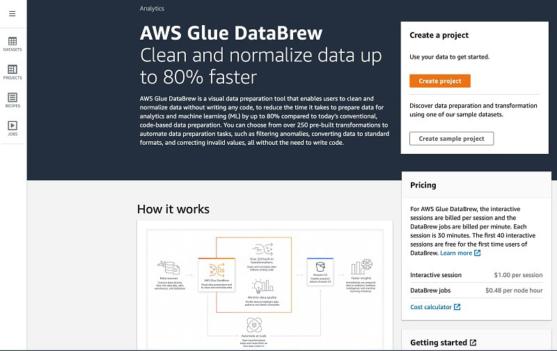
AWS Glue DataBrew is a visual data preparation tool that helps solve some of these challenges by allowing you to inspect datasets and apply transformations against them in a visual and no code way that allows users of all skill sets to participate as part of the data preparation pipeline process. An obvious benefit is data owners and SMEs (subject matter experts) can define and implement data quality and governance checks against their data before publishing it into the data lake.

This accelerates and simplifies the process of producing trusted and quality outputs because the data owners are integrated as part of the onboarding process.

For this post, we discuss a use case of a project team in a consultancy organization that wants to combine first-party data they have acquired against an existing dataset that exists within their data lake.

Overview of solution

The workflow includes the following steps:

Step 1: Create a new AWS Glue DataBrew dataset by uploading a file to, or choosing and existing dataset, from their organization data lake.
Step 2: Create a DataBrew project to load and visually inspect and validate the datasets that you will transform.
Step 3: Using DataBrew, visually transform, augment and define the business rules you want to be applied to your new dataset. (These business rules are called steps, which collectively are called a Recipe)
Step 4: Create a DataBrew job to execute your Rules (Recipe) against the datasets in their entirety.
Step 5: Run a AWS Glue crawler to discover the resulting dataset, publish it to the AWS Glue data catalog and apply a secure permission model to it.
Step 6: Use a preferred analysis or machine learning (ML) tool to browse and consume the data in the Data Catalog based on user permissio

Let’s now go through these steps in a bit more detail.

Creating a project

A project in DataBrew defines two key aspects: the primary dataset you’re working with and the steps you want to run against that dataset to produce a trusted and validated dataset that is specific to your business need.

To create your project, complete the following steps:

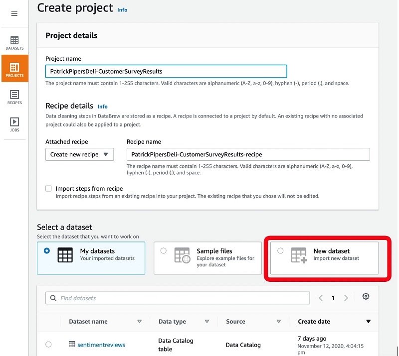
  1. On the DataBrew console, choose Create project.


  1. For Project name, enter a name that is representative of the source and intent of the output.
  2. For Attached recipe, choose Create new recipe.

In subsequent projects with a similar shape of data, you can reuse your recipe of business rules.

You have several options when connecting your dataset. You can upload a new data source (such as a local Excel or JSON file on my computer) or to reuse an existing dataset that exists within your data lake. If you’re sourcing data from the data lake, you can filter by the origin of the source, such as our cloud data warehouse Amazon Redshift, or transactional systems hosted in an Amazon Relation Database Service (Amazon RDS) instance. For more information about copying data into your data lake using AWS Glue, see Which Data Stores Can I Crawl? For this post, I upload a new dataset.

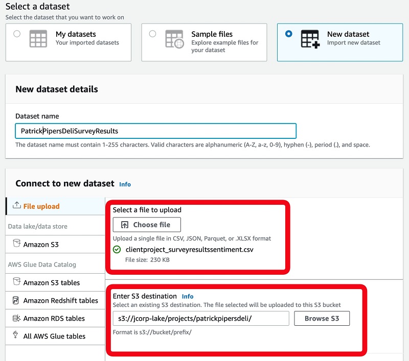
  1. Select New dataset.

  1. For Dataset name, enter a name.
  2. For File upload, choose Choose file.
  3. Choose the file to upload.
  4. For Enter S3 destination, enter the location in our data lake where the file is saved to.

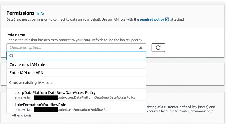
  1. For Role name, choose a security role that grants access to the data lake location specified.

Typically, this is an area that you have access to that is driven by project or department privileges.

If no role is provided by default, a data platform admin or AWS account admin can create one for you. For more information, see Identity-based policy examples for AWS Glue DataBrew.

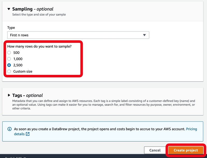
  1. Optionally, modify the sample size of the data to inspect.
  2. Choose Create project.

Analyzing and transforming your dataset

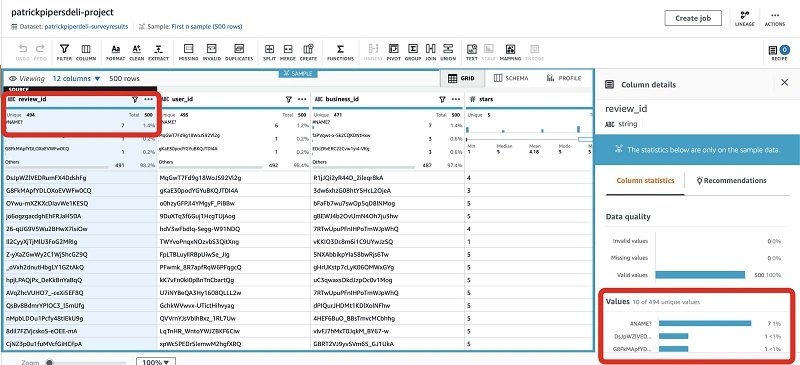
With a project created, I can load a sample of my dataset in a familiar tabular grid view and start to explore the data in greater detail.

This view allows for quick inspection of the data and the ability to run some sample and survey methods to determine if the data being viewed has statistical significance to our project. This way, we can make sure we’re making informed, data-driven decisions on behalf of our clients.

The following screenshot shows that the review_id column has duplicate values.

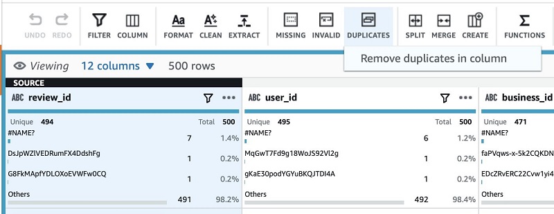
To maintain integrity and trust of the output, I can remove the duplicate rows as a step by choosing Duplicates and Remove duplicates in column.

This adds a new step to my recipe, which is enforced on this column type whenever it runs. DataBrew shows a preview of the change before you apply the changes. 

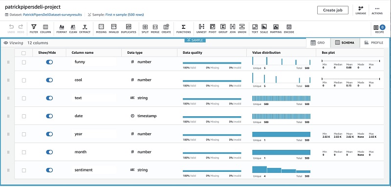
If I want to dig deeper into the shape and validity of my data, I can simply choose the Schema tab to get a coalesced view of the data, or create a data profile job on the Profile tab to get further insights, such as correlations across column types.

The rest of the data looks good, so I now complete the rest of my transformation functions:

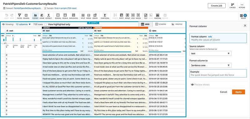
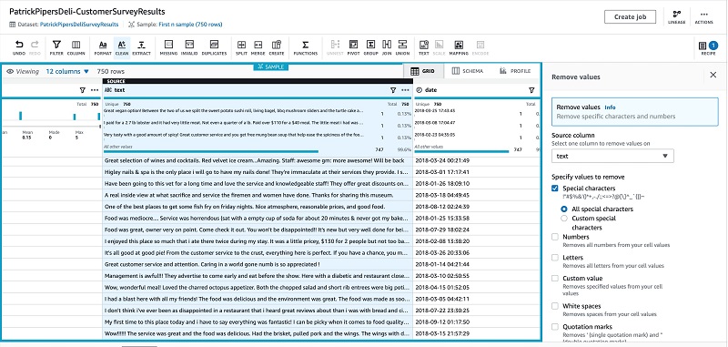
  1. Clean the survey result summary text by removing invalid characters and quotes, and enforcing sentence casing.
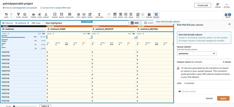
  2. For downstream ML tasks, apply a hot encode function to the text value of a customer’s sentiment (categorical variable) to that of an integer value (binary vector).
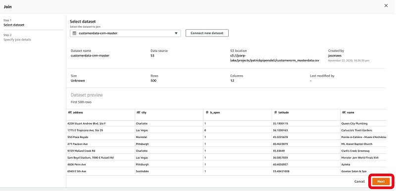
  3. Join to a company dataset that contains our customer data so I can bring in identifiable information of the locations surveyed.
  4. Hide columns not require for the final output.

Cleaning the summary text

We first clean the survey result summary text by removing invalid characters and quotes, and enforce sentence casing.

  1. Choose Format.
  2. Choose Change to sentence casing.

  1. On the recipe bar, choose Clean.
  2. For Specify values to remove, select Special characters.

Applying a hot encode function

Next, apply a hot encode function to the categorical variable (sentiment) to a binary vector for downstream ML purposes.

  1. Choose Encode.
  2. Choose One-Hot-Encode column.
  3. Choose your source column.
  4. Choose Apply.

Joining and enriching our dataset

We now join our dataset against a primary customer dataset so we can enrich our dataset with additional columns of value.

The initial dataset we created contains a number of key data elements, such as a review rating, customer comments, associated sentiment rating, a number of ordinal values specifying the value of the review, emotional attributes from the interviewee, and various restaurant and location identifiers.

As part of our full analysis, we want to reference the additional data elements associated with these restaurant and location identifiers so we can form a complete view of the data.

DataBrew makes this enrichment task easy by letting you join to an additional company dataset that exists within your data lake. In the following steps, I choose to bring across only those columns that I require by deselecting those that are not required. (This existing dataset contains additional data of businesses that are part of the wider survey group.)

  1. On the recipe menu bar, choose Join.
  2. Choose Dataset join.
  3. For Select dataset, choose the dataset to join against.

The page displays a summary view for inspection.

  1. Choose Next.

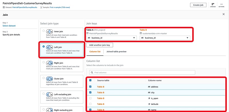
For this post, we perform a left join to ensure that we’re only bring in matching records against our own dataset (Table A) from the paired dataset (Table B).

  1. Choose the columns between both tables that we want to match against (for this post, business_id).
  2. Select the columns from the joined table to include in our dataset.

  1. Choose Finish.

When this step is complete, we have a complete dataset that is applicable towards our final requirements for analysis.

Removing unnecessary columns

Finally, remove columns not required for the final dataset and change the column names. ­­

At the conclusion of our data preparation, we can see the number and types of steps we have run.

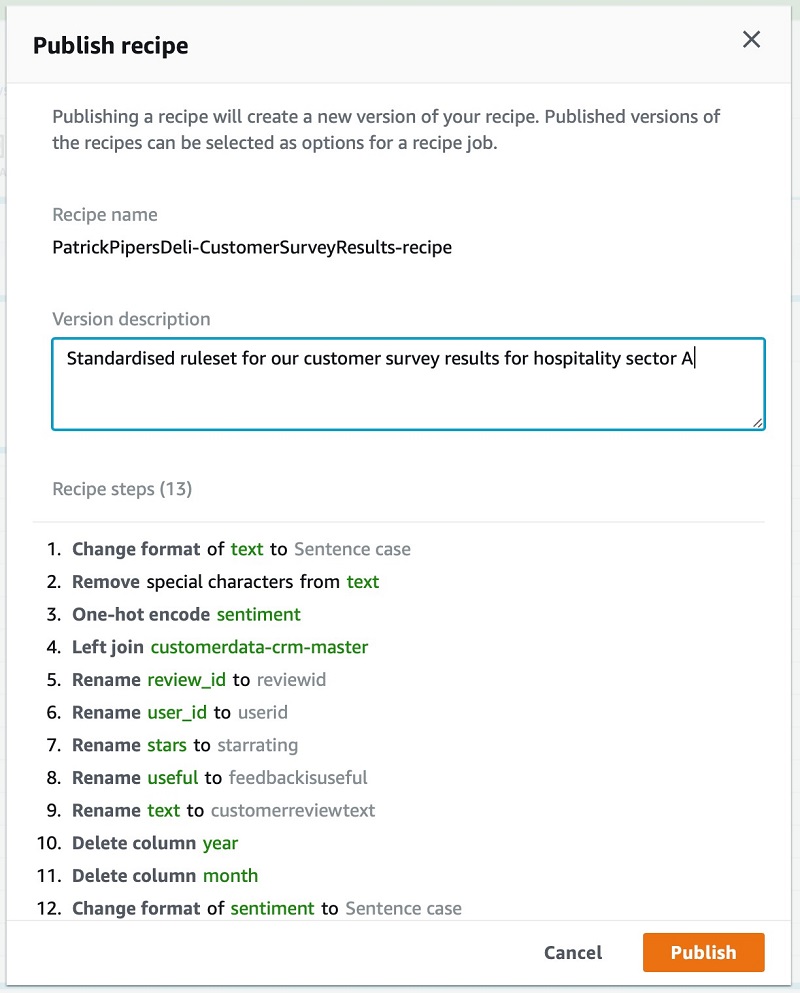
For similar datasets, you can choose Publish in the Recipe pane to reuse this recipe and enforce the steps taken instead of having to complete the steps again. This allows you to build up your own repository of recipes that you can replay against various datasets to ensure a consistent level of data quality and outputs.

You then provide a description and publish the recipe for broader accessibility.

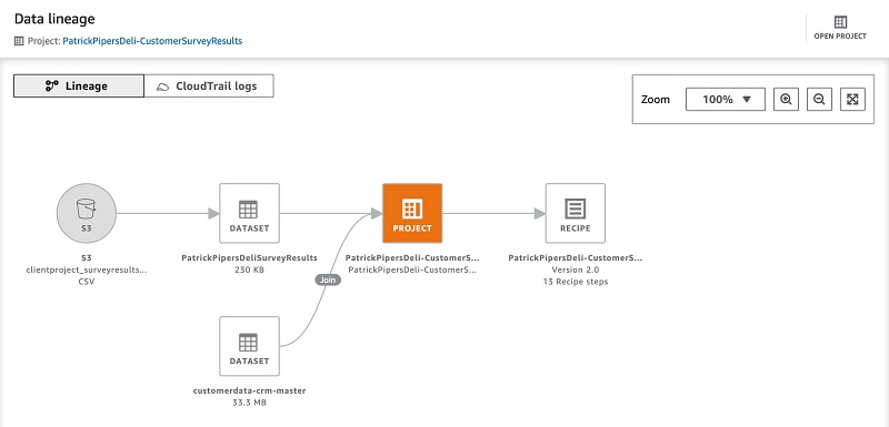
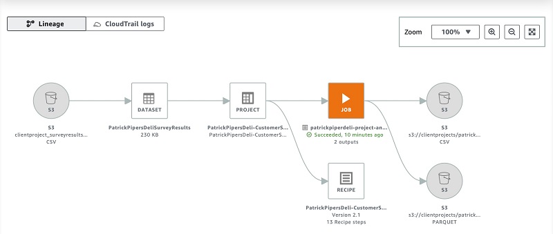
As a final validation step before publishing my dataset, I can choose to visually inspect the data lineage to confirm my sources selected are as intended and to confirm the size of my datasets to process.

For this post, I can confirm that the source and datasets are correct and the recipe being created has the expected number of steps. The data lineage view is useful for when you’re reading unfamiliar data sources because it allows you to understand the origins and transformations that have taken place beforehand.

Creating a job to publish your dataset

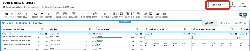
Now we have our dataset defined and validated by way of the visual steps we created in our recipe. It’s time to create a job that runs them against the entirety of our dataset. The output is saved back into an area of our data lake for additional processing, leading to publication within our Data Catalog.

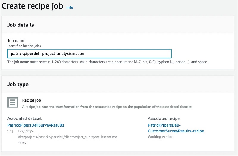
  1. Choose Create job.

  1. For Job name, enter a name.

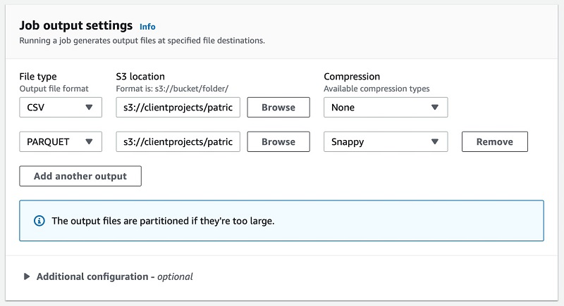
  1. In the Job output settings section, specify the data lake location where the final output is saved to.

If required, we can optionally choose a file format for the dataset. If you have multiple requirements for different file formats, you can simply choose to save multiple outputs by choosing Add another output and specifying the details. For this post, I opt to save the output in two formats: one in CSV and another in the optimized open file format Apache Parquet.

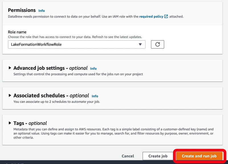
  1. For Role name, choose the security role that has access to our client project folder to make sure DataBrew has permission to save the dataset to the location specified.

The role that you choose here is different than the DataBrew role you chose when creating the project. Each role serves a different purpose. For this post, we choose a role that has permissions to read, run, and save the resulting files into data lake locations (as governed by the role) of which I have been delegated rights to access and save data to.

  1. Choose Create and run job.


The project is now visible on the main page, detailing the recipe used against the dataset and the job name.
style=”margin: 20px 0px 20px 0px; border: 1px solid #CCCCCC;”

To view details about the job run and inspect completion details, choose the value in the Jobs column.

To see additional details about the history of the job, choose the job name.

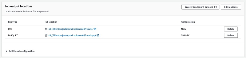
The output provides details of the job.

The lineage view shows the end-to-end process of all input files, transformation steps, and final output locations.

Consuming your dataset

After you save the new dataset to your data lake, we can use AWS Glue to crawl the new dataset and publish it to our Data Catalog. For more information, see Populating the AWS Glue Data Catalog. After the data is indexed, it’s available and visible through AWS Glue and Lake Formation. 

Crawling the output files from DataBrew

To crawl the output files and publish them to our Data Catalog, complete the following steps:

  1. On the AWS Glue console, choose Crawlers.
  2. Choose Add crawler.

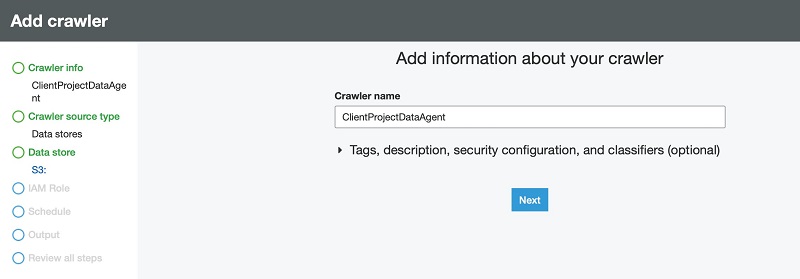
  1. For Crawler name, enter a name.
  2. Choose Next.

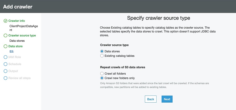
  1. For Crawler source type, select Data stores.
  2. For Repeat crawls of S3 data stores, select Crawl new folders only.
  3. Choose Next.

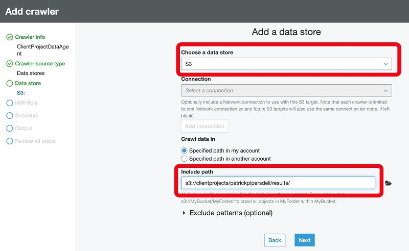
  1. For Choose a data store, choose S3.
  2. For Crawl data in, select Specified path in my account.
  3. For Include path, enter the path of the DataBrew output files.
  4. Choose Next.

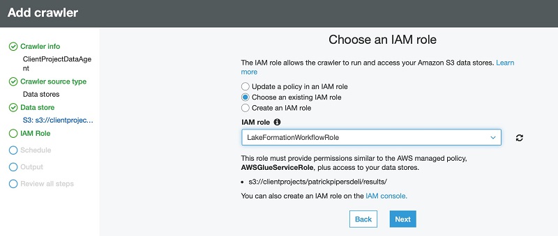
  1. Select Choose an existing IAM role.
  2. For IAM role, choose or create a role that has access to the location of your DataBrew output.

If you don’t have such a role, your data platform admin can set one up for you.

  1. Choose Next.

  1. For Frequency, specify how often the crawler should check for new output files. For this post, we choose Run on demand. 

This normally aligns with the schedule you have set up in DataBrew.

  1. Choose Next.
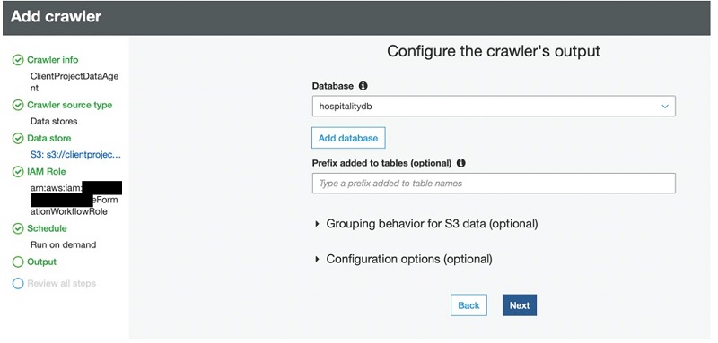
  2. For Database, choose (or create) a database to publish the business view of your output files.

The crawler creates one or more data tables that users can browse and, if permissions allow, run select queries against.

  1. Choose Next.

  1. Review the summary page and choose Finish.
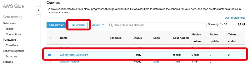
  2. Select your crawler and choose Run crawler.

When the crawler is complete, it details the number of tables it created and the time it took to discover and index your output dataset. The next step is to view and set up permissions in the Data Catalog.

Publishing and securing your DataBrew output files

In this post, we use the Lake Formation security and permission model enforced for data consumers using supported services. For more information, see Security and Access Control to Metadata and Data in Lake Formation.

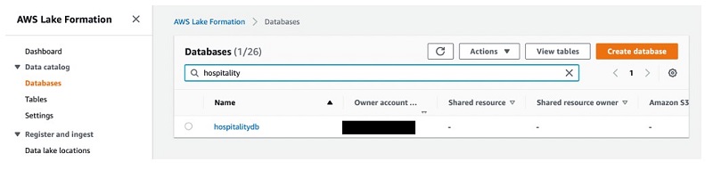
  1. On the Lake Formation console, under Data catalog, choose Databases.
  2. Enter the database name you used when you created the crawler earlier (for this post, hospitalitydb).


  1. Select the database and choose View tables.

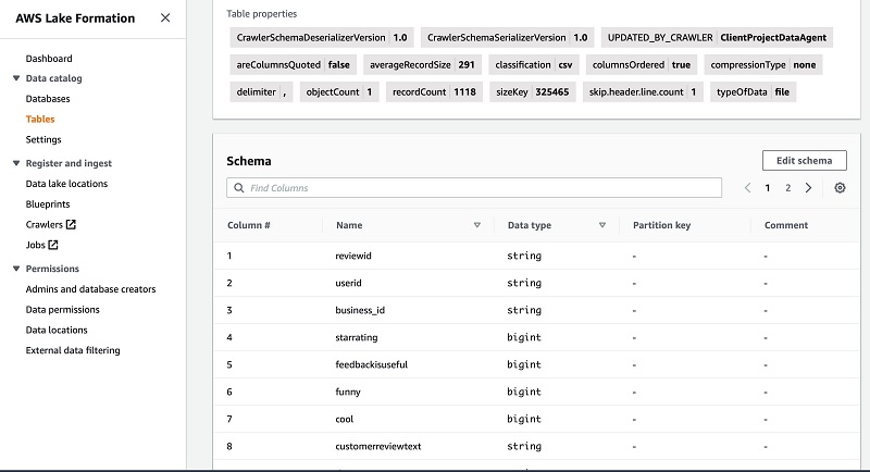
We can see that a table called results was created in this database.

We can do several things, such as grant or revoke items from the Actions menu, or choose the table name to inspect the schema.

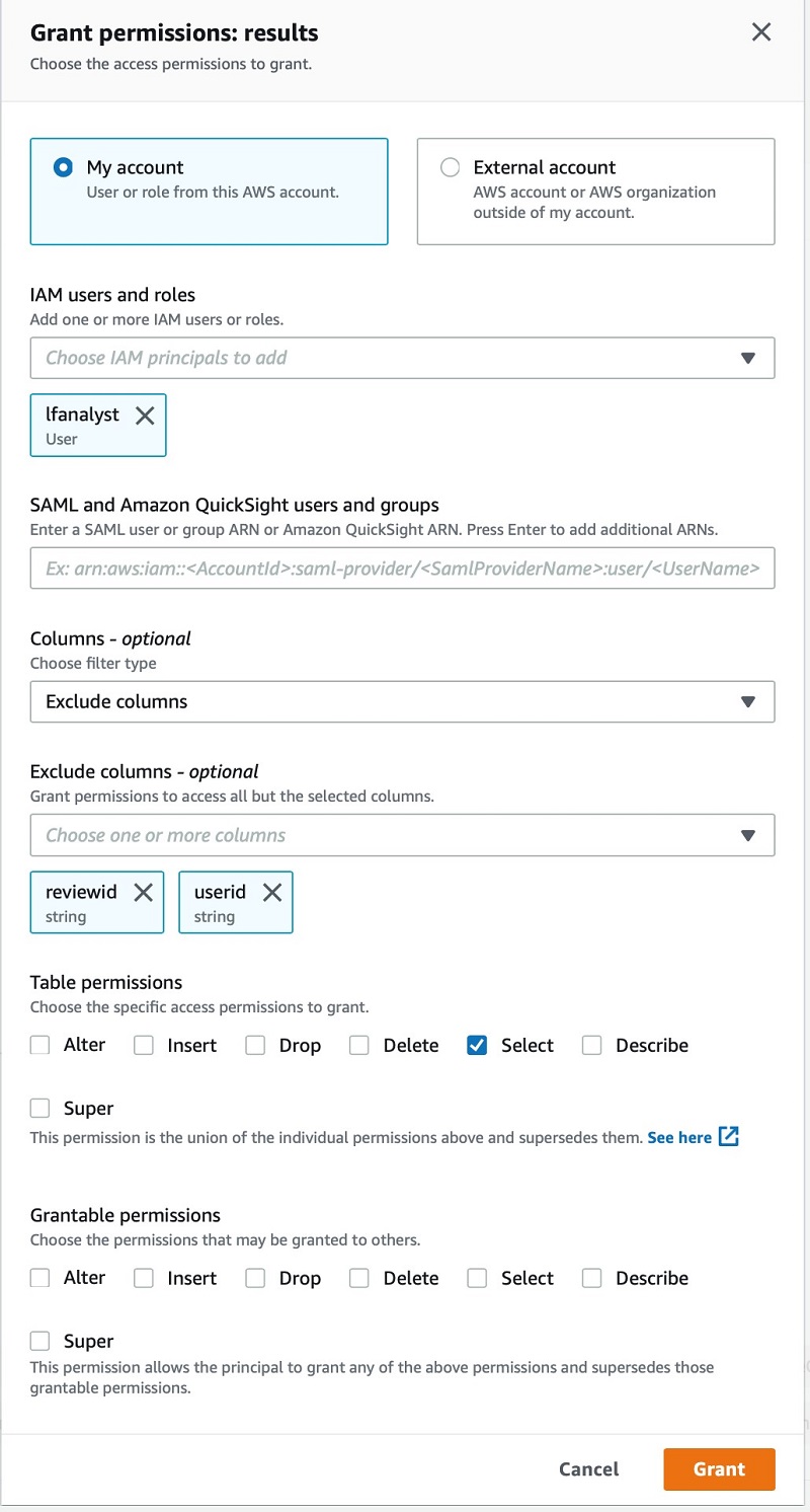
As a data owner, I grant an analyst with the username lfanalyst select permissions to my dataset, and restrict access to only a limited set of columns. For this post, I exclude the userid and reviewid columns.

After I save this change, I can let the analyst know that they have access to my survey results.

Consumption access to DataBrew output files

The analyst user who has been granted limited access to this dataset can query the data using Amazon Athena, either via the console or external analytical tools that support the JDBC or ODBC drivers it provides.

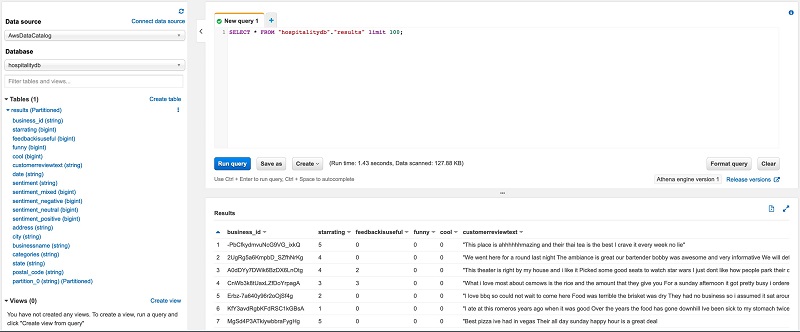
If using the console, the analyst can choose the database hospitalitydb to view the results table.


If the analyst expands the results table to view the columns, userid and reviewid aren’t present.

The following screenshot shows the results of a SQL statement to browse a sample of the dataset.

Conclusion

DataBrew makes it easy for data owners, analysts, and data SMEs to easily curate and publish data of value to their organization data lake in a self-service manner.

This visual interface, combined with ML assistance to help you better understand and validate your data, allows all types of users to easily create, consume, and publish data into an organization’s data lake in a visual, no code, or low code way while working within an existing centralized governance model.


About the Author

Jason Hunter is a Principal Solutions Architect at AWS with a focus on Big Data & Analytics solutions. With over 20 years of experience in information technology, he helps customers architect and build highly scalable, secure and performant cloud-based data platforms, accelerating their journey to become more data driven.