Post Syndicated from Aritra Nag original https://aws.amazon.com/blogs/architecture/build-priority-based-message-processing-with-amazon-mq-and-aws-app-runner/
Organizations need message processing systems that can prioritize critical business operations while handling routine tasks efficiently. When handling time-sensitive tasks like rush orders from key customers, critical system alerts, or multi-step business processes, you need to prioritize urgent messages while making sure other routine requests are processed reliably.
In this post, we show you how to build a priority-based message processing system using Amazon MQ for priority queuing, Amazon DynamoDB for data persistence, and AWS App Runner for serverless compute. We demonstrate how to implement application-level delays that high-priority messages can bypass, create real-time UIs with WebSocket connections, and configure dual-layer retry mechanisms for maximum reliability.
This solution addresses three critical challenges in modern data processing systems:
- Implementing configurable delay processing at the application level
- Supporting priority-based message routing that respects business requirements
- Providing real-time feedback to users through WebSocket connections
The use of AWS managed services reduces operational complexity, so teams can focus on business logic rather than infrastructure management. Message handling with priority-based processing makes sure operations receive attention while routine tasks are processed in the background. Users will experience status updates that provide visibility into their requests, while retry mechanisms provide reliability during failures. The infrastructure as code (IaC) approach supports deployments across different environments, from development through production.
Solution overview
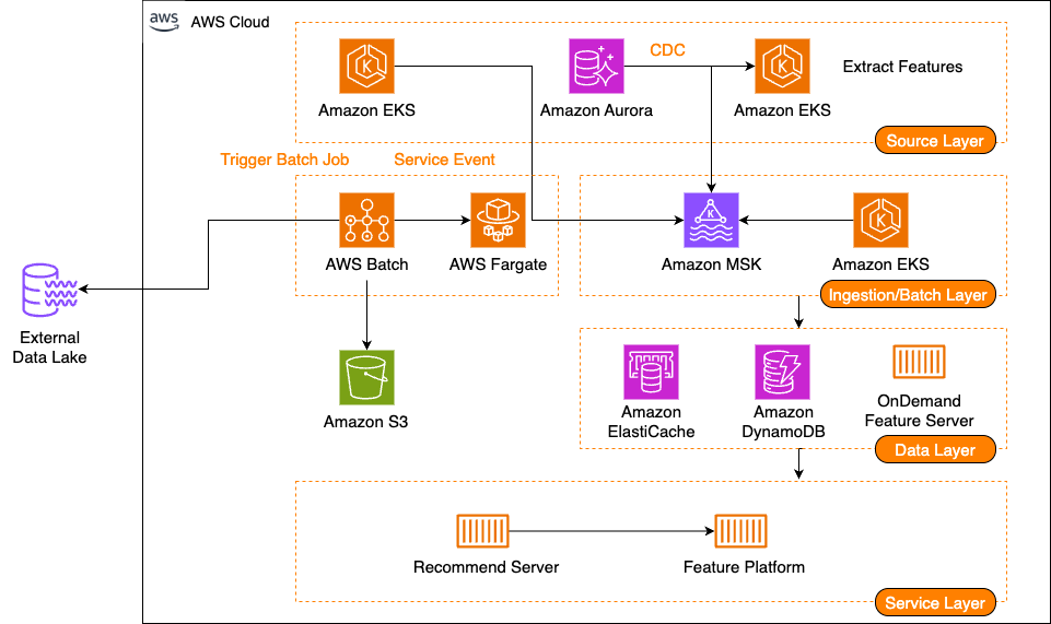
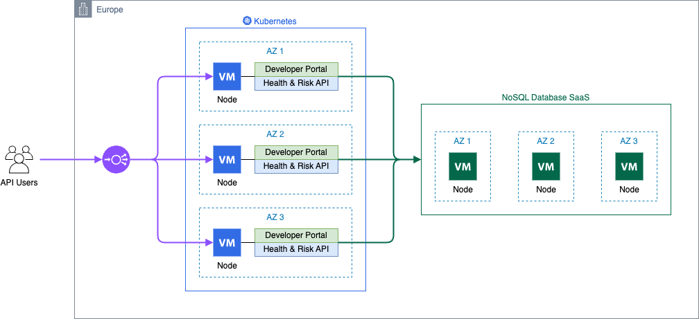
The solution consists of several AWS managed services to create a serverless, priority-based message processing system with real-time user feedback. The architecture implements intelligent routing based on three message priority levels, to make sure critical messages receive immediate processing:
- High-priority path – Messages bypass delays and queue immediately with JMS priority 9
- Standard-priority path – Messages undergo configured delays before queuing with JMS priority 4
- Low-priority path – Messages process after all higher priority messages with JMS priority 0
The following diagram illustrates this architecture.
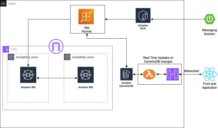
The solution uses the following AWS managed services to deliver a scalable, serverless architecture:
- AWS App Runner is a fully managed container application service that automatically builds, deploys, and scales containerized applications. It provides automatic scaling based on traffic, built-in load balancing and HTTPS, seamless integration with container registries, and zero infrastructure management overhead.
- Amazon MQ is a managed message broker service for Apache ActiveMQ that offers priority-based message queuing, automatic failover for high availability, message persistence and durability, and JMS protocol support for enterprise applications.
- Amazon DynamoDB is a fully managed NoSQL database service providing single-digit millisecond performance at any scale, automatic scaling with on-demand pricing, built-in security and backup capabilities, and global tables for multi-Region deployments.
The system uses JMS priority levels with High=9, Medium=4, and Low=0 for automatic ordering, combined with conditional delay processing based on priority classification. Amazon MQ provides reliable message delivery and persistence with dead-letter queue (DLQ) configuration for failed message handling.
Asynchronous delay processing uses CompletableFuture implementation for non-blocking delays, thread pool management for concurrent processing, graceful error handling with retry mechanisms, and configurable delay periods per message type to optimize resource utilization. For real-time status updates, the solution provides WebSocket connections for bidirectional communication, Amazon DynamoDB Streams for change data capture (CDC), comprehensive status tracking throughout the processing lifecycle, and a React frontend integration for live updates, so users have complete visibility into their message processing status.
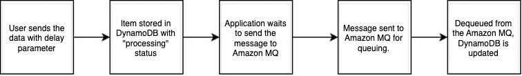
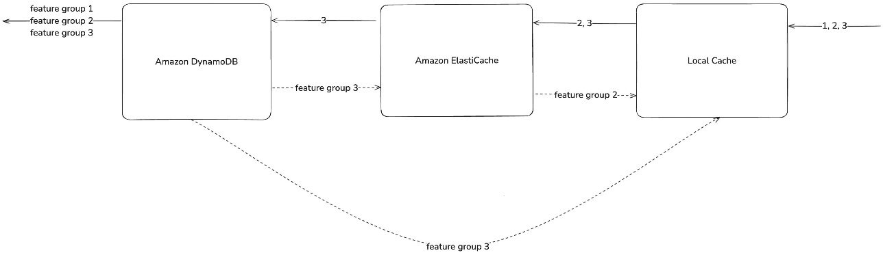
The standard priority messaging flow (shown in the following diagram) handles messages with configurable delays using JMS asynchronous processing capabilities. Messages wait for their specified delay period before entering the Amazon MQ queue, where they’re processed.
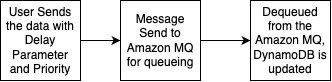
The high-priority messaging flow (shown in the following diagram) provides an express lane for critical messages. These messages skip the delay mechanism entirely and proceed directly to the queue, providing immediate processing for time-sensitive operations.
To make it even more straightforward to get started, we’ve prepared an example application that you can use to observe the Amazon MQ behavior with varying message volumes. You can find the source code repository, IaC implementation, and instructions to run the sample on GitHub.
In the following sections, we walk you through deploying the complete processing system.
Prerequisites
Make sure you have the following tools, permissions, and knowledge to successfully deploy the priority-based message processing system. You must have an active AWS account with the following configurations:
- The AWS Command Line Interface (AWS CLI) version 2.15.0 or later
- AWS Identity and Access Management (IAM) roles with the minimum permissions:
Install and configure the following development tools on your local machine:
- Java 17 or later
- Spring Boot 3.2.0 or later
- Node.js 18.19.0 or later
- Docker 24.0.7 or later
- Maven 3.9.6 or later
- AWS CDK 2.124.0 or later
To successfully implement this solution, you should have basic familiarity with the following:
- Spring Boot applications
- Message queue concepts
- WebSocket protocols
- React development
Configure the infrastructure stack
This step involves creating the core AWS services using the AWS Cloud Development Kit (AWS CDK). This modular approach enables independent stack management and environment-specific configurations.
- Create a new AWS CDK project:
- Create the infrastructure stack:
- Run the following commands to deploy the stack:
You can verify the infrastructure on the AWS Management Console.
Configure the message processing application
In this step, we create the Spring Boot application with priority-based message processing capabilities. First, we configure the application.properties file to incorporate environment variables, including AWS credentials, AWS Regions, and other configuration parameters such as log levels into the application and business logic implementation. Next, we implement the message service using a JMS template with comprehensive error handling, followed by enhancing the JMS configuration with connection pooling for improved performance.
The following code illustrates an example message service implementation:
For proper timestamp update implementation, we integrate the DynamoDB SDK service with caching capabilities. Finally, after implementing the REST controller for the API with asynchronous processing support, we can deploy the message processing application. This implementation includes Java code application-level delay processing for demonstration purposes. Although this approach effectively showcases the priority-based message routing capabilities and real-time WebSocket updates in our demo environment, AWS recommends using Amazon MQ delay processing features for production workloads. For production implementations, use Amazon MQ delay and scheduling capabilities instead of application-level delays through features like Amazon MQ delay queues, ActiveMQ scheduling features, and appropriate message Time-to-Live (TTL) configurations.
The following code is an example snippet showcasing the Amazon MQ feature:
Build and deploy the Spring Boot application to App Runner
In this step, we push the application to Amazon Elastic Container Registry (Amazon ECR) to run it in App Runner:
- Build and push the Docker image to Amazon ECR:
- Create the App Runner service with environment variables for the DynamoDB table and Amazon MQ broker endpoint:
Set up real-time updates
For this step, we implement WebSocket support for real-time status updates using AWS Lambda to process DynamoDB streams and send updates to connected clients using Amazon API Gateway WebSocket connections. You can find the code snippet for this in this link
Deploy the React application to Amazon S3 and Amazon CloudFront
In this step, we create a frontend application to enable the WebSocket connection for seeing the messaging getting updated in the DynamoDB and API Gateway WebSocket connections.
Similar to the above section, here is the AWS cdk code for building the frontend for proceeding towards the validation of the solution
Validate the solution
This section provides comprehensive testing procedures to validate the priority-based message processing system.
Automated testing script
After you have completed the preceding steps, you can initiate a comprehensive testing script to validate priority processing and delay behavior:
Validation through the web interface
The following screenshot of the UI illustrates how the queueing mechanism can work with the real-time updates using WebSockets.
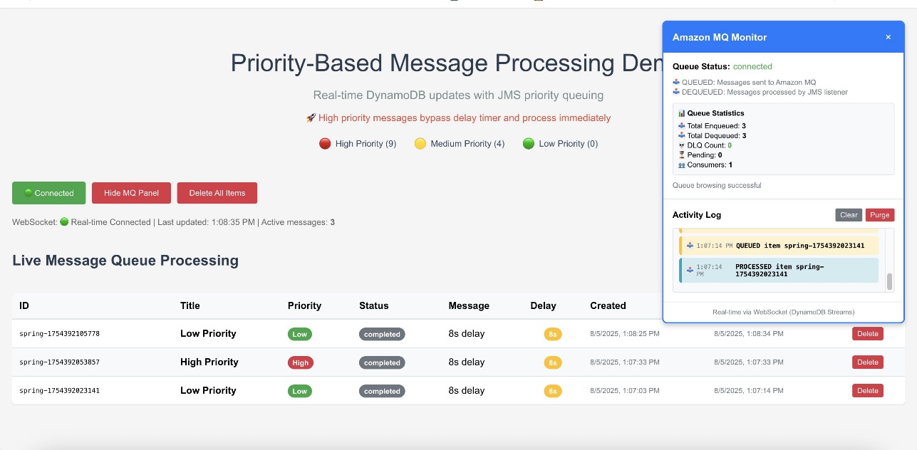
The web interface provides validation of the priority-based message processing system. Access the Amazon CloudFront URL to view the following information:
- Real-time message processing with live status updates
- Queue statistics showing message distribution by priority
- Processing timeline demonstrating priority bypass behavior
- WebSocket connection status indicating real-time connectivity
Amazon CloudWatch dashboards and alarms
AWS recommends creating Amazon CloudWatch dashboards to track your priority-based message processing system’s performance across multiple dimensions. Monitor message processing by priority levels to make sure high-priority messages are processed first and identify any bottlenecks in your priority routing logic. The following screenshot shows an example dashboard.
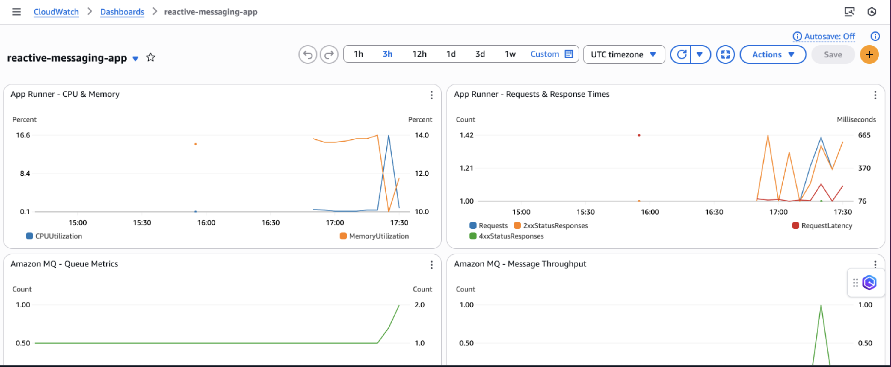
You can track queue depth and processing times to understand system load and latency patterns, helping you optimize resource allocation and identify when scaling is needed. Observe DynamoDB performance metrics including read/write capacity consumption, throttling events, and latency to make sure your database layer maintains optimal performance under varying loads.
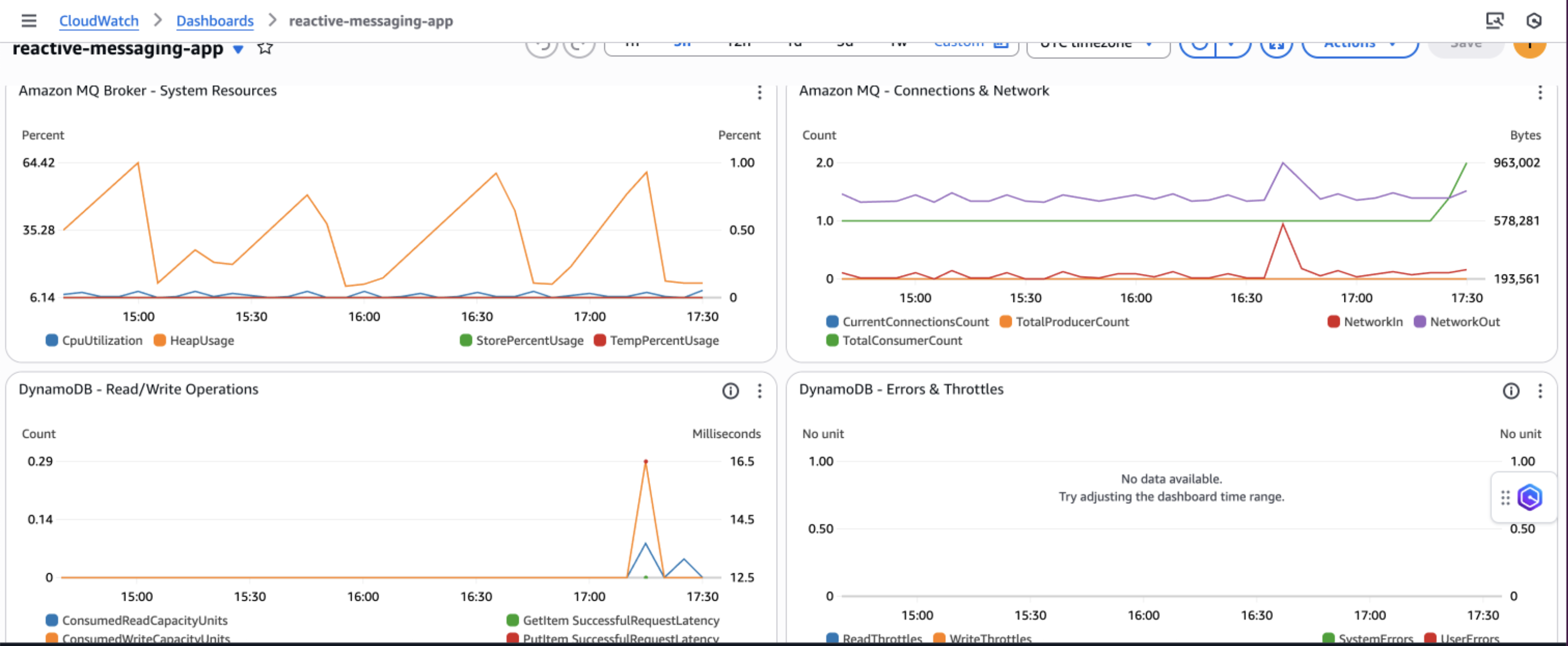
Additionally, implement application-specific custom metrics such as message processing success rates, retry counts, and business-specific KPIs to gain deeper insights into your application’s behavior and make data-driven decisions for continuous improvement.
Security considerations
AWS recommends implementing comprehensive security measures to safeguard your message processing system. Start by implementing least privilege IAM policies that grant only the minimum permissions required for each component to function, making sure services like App Runner can only access the specific DynamoDB tables and Amazon MQ queues they need. Configure your network architecture using a virtual private cloud (VPC) with private subnets for Amazon MQ, isolating your message broker from direct internet access while maintaining connectivity through NAT gateways for necessary outbound connections.
Enable encryption at rest using AWS Key Management Service (AWS KMS) for DynamoDB tables and Amazon MQ data and enforce encryption in transit by configuring SSL/TLS connections for all service communications, particularly for ActiveMQ broker connections. Finally, configure security groups with minimal access rules that explicitly define allowed traffic between components, restricting inbound connections to only the ports and protocols required for your application to function, such as port 61617 for ActiveMQ SSL connections from App Runner instances.
Cost considerations
The following table contains cost estimates based on the US East (N. Virginia) Region. Actual costs might vary based on your Region, usage patterns, and pricing changes.
| Service | Small (1,000 msg/day) | Medium (10,000 msg/day) | Large (100,000 msg/day) |
| Amazon DynamoDB | $5–10 | $25–50 | $200–400 |
| Amazon MQ | $15 (t3.micro) | $30 (m5.large) | $120 (m5.xlarge) |
| AWS App Runner | $20–40 | $50–150 | $400–800 |
| Amazon API Gateway WebSocket | $3–5 | $10–25 | $50–100 |
| Amazon CloudWatch Logs | $5–10 | $10–20 | $30–50 |
| Data Transfer | $5 | $10-20 | $50-100 |
| Total Estimated Cost | $53–95 | $135–295 | $850–1,570 |
Troubleshooting
The following are common issues and their solutions when implementing the priority-based message processing system:
- Messages not processing in priority order:
- Verify JMS priority is configured correctly:
message.setJMSPriority(priority) - Check ActiveMQ broker configuration for priority queue support
- Confirm
CLIENT_ACKNOWLEDGEmode is properly configured - Review queue consumer concurrency settings
- Verify JMS priority is configured correctly:
- WebSocket updates not working:
- Verify DynamoDB Streams is enabled on the table
- Check the Lambda function is triggered by stream events
- Validate API Gateway WebSocket configuration and IAM permissions
- Test the WebSocket connection using browser developer tools
- Application scaling issues:
- Monitor App Runner metrics in CloudWatch
- Adjust auto scaling configuration based on traffic patterns
- Consider Amazon MQ broker capacity and upgrade if needed
- Review DynamoDB capacity settings and enable auto scaling
Clean up
To avoid incurring ongoing AWS charges, delete the resources you created in this walkthrough:
- Delete the CDK stacks:
- Remove the App Runner service:
- Delete the ECR repositories and container images.
- Remove CloudWatch log groups if not set to auto-delete.
- Delete S3 buckets used for frontend hosting.
Next steps
To extend this solution and add additional capabilities, consider the following enhancements:
- Integrate AWS Step Functions for complex workflow orchestration
- Add Amazon EventBridge for event-driven integrations
- Implement Lambda for serverless message processing
- Use Amazon SageMaker for ML-based priority classification
- Build dashboards with Amazon QuickSight for business intelligence
Conclusion
This solution demonstrates how to build a production-ready priority-based message processing system using AWS managed services. By combining Amazon MQ priority queuing with DynamoDB real-time streams and App Runner serverless compute, you create a resilient architecture that intelligently handles messages based on business priorities.The implementation of application-level delays with priority bypass makes sure critical messages receive immediate attention, and the dual-layer retry mechanism provides maximum reliability. Real-time WebSocket updates keep users informed of processing status, creating a responsive and transparent system.To learn more about the services and patterns used in this solution, explore the following resources:
- AWS documentation and guides:
- Reference architectures and solutions:
- Video tutorials:


 As we move into the second week of 2025, China is celebrating Laba Festival (腊八节), a traditional holiday, which marks the beginning of Chinese New Year preparations. On this day, Chinese people prepare


 Raghu Kuppala is an Analytics Specialist Solutions Architect experienced working in the databases, data warehousing, and analytics space. Outside of work, he enjoys trying different cuisines and spending time with his family and friends.


 Diego Colombatto is a Senior Partner Solutions Architect at AWS. He brings more than 15 years of experience in designing and delivering Digital Transformation projects for enterprises. At AWS, Diego works with partners and customers advising how to leverage AWS technologies to translate business needs into solutions.
 Angel Conde Manjon is a Sr. EMEA Data & AI PSA, based in Madrid. He has previously worked on research related to Data Analytics and Artificial Intelligence in diverse European research projects. In his current role, Angel helps partners develop businesses centered on Data and AI.
 Tiziano Curci is a Manager, EMEA Data & AI PDS at AWS. He leads a team that works with AWS Partners (G/SI and ISV), to leverage the most comprehensive set of capabilities spanning databases, analytics and machine learning, to help customers unlock the through power of data through an end-to-end data strategy.


