All posts by Raghu Kuppala

Getting started with Apache Iceberg write support in Amazon Redshift – Part 3

Post Syndicated from Raghu Kuppala original https://aws.amazon.com/blogs/big-data/getting-started-with-apache-iceberg-write-support-in-amazon-redshift-part-3/

Production data is always evolving. Tables gain and lose columns, outgrow their data types, and get re-partitioned as query patterns shift. Multiple engines often need to read the same data. These changes used to mean expensive data rewrites or rebuilt pipelines. Apache Iceberg makes them metadata-only operations, and Amazon Redshift now supports evolving schemas and partitioning layouts through ALTER statements, with no data rewrites and no pipeline rebuilds. You can also create AWS Lake Formation resource links in the catalog of Amazon S3 Tables, a capability of Amazon Simple Storage Service (Amazon S3), for centralized cross-engine governance.

In Part 1, you created Apache Iceberg tables and wrote data directly from Amazon Redshift to your data lake, setting up external schemas, creating tables in both Amazon Simple Storage Service (Amazon S3) and Amazon S3 Tables, and performing INSERT operations with full ACID (Atomicity, Consistency, Isolation, Durability) compliance. In Part 2, you performed DELETE, UPDATE, and MERGE operations to modify data at the row level and synchronize staging and production tables.

In this post, you use the customer and orders datasets from the previous posts to evolve Iceberg table schemas and partitioning with ALTER operations. You also create an AWS Lake Formation resource link in the S3 Tables catalog to share tables with other analytics engines under a single, centralized permission model.

Solution overview

This solution demonstrates ALTER operations for Apache Iceberg tables in Amazon Redshift and Lake Formation resource link creation for the S3 Tables catalog. The walkthrough includes the following key operations:

  • ALTER TABLE RENAME COLUMN – Rename existing columns without changing data types or partition specs.
  • ALTER TABLE ADD/DROP COLUMN – Add new columns or remove existing columns as metadata-only operations.
  • ALTER TABLE ALTER COLUMN – Widen column data types (for example, INT to BIGINT) without rewriting data.
  • ALTER TABLE SET TABLE PROPERTIES – Change compression type for future writes.
  • ALTER TABLE ADD/DROP/REPLACE PARTITION FIELD – Evolve partition specs without re-partitioning existing data.
  • Lake Formation resource link – Create a resource link in the S3 Tables catalog for centralized access governance.

The following diagram shows the end-to-end architecture:
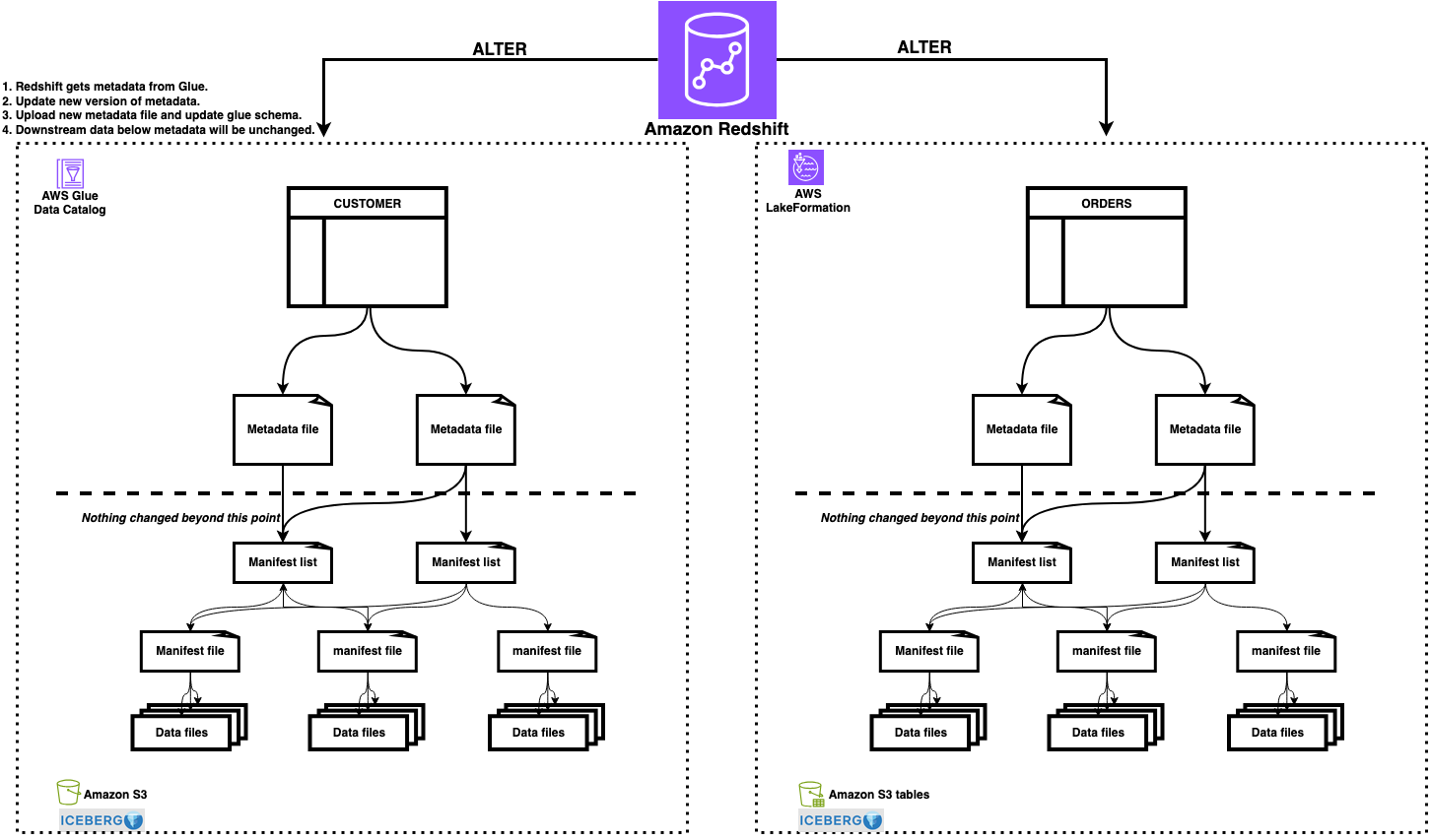
Architecture diagram of Amazon Redshift running ALTER operations on Iceberg tables in S3 Tables, with Lake Formation resource links providing access from Amazon Athena and other engines

Figure 1: Architecture showing Amazon Redshift performing ALTER operations on Iceberg tables in S3 Tables, with Lake Formation resource links providing access from Amazon Athena and other engines

Prerequisites

Complete the setup from Part 1 and Part 2, including:

  • An Amazon Redshift data warehouse (provisioned or Serverless) on patch 201 or higher.
  • The AWS Identity and Access Management (IAM) role (RedshifticebergRole) with permissions for Amazon S3, AWS Glue Data Catalog, and Lake Formation.
  • The customer table in a standard Amazon S3 bucket (AWS Glue catalog: customer_db).
  • The orders table in an Amazon S3 table bucket (iceberg-write-blog@s3tablescatalog).
  • Access to an IAM role that is a Lake Formation data lake administrator.
  • AWS Glue Data Catalog integrated with S3 Tables (s3tablescatalog exists).

Schema evolution with ALTER TABLE

With ALTER TABLE, you can change Iceberg table definitions, including schema, partition specs, and properties, without rewriting stored data. Each operation updates only metadata. The table structure changes instantly while existing data files remain untouched. This helps make schema evolution, partition adjustments, and property updates safe to run on production tables.

Add a column

You can add a new column to an Iceberg table using ALTER TABLE. Each new column is added with a unique field ID that Iceberg uses for column tracking across schema evolution. Existing rows return NULL for the newly added column.

Verify the current schema:
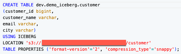
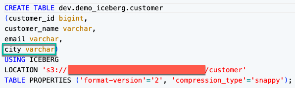
SHOW TABLE dev.demo_iceberg.customer;
SHOW TABLE output listing the current columns of the customer table

Figure 2: SHOW TABLE output showing the current customer table schema

Add the column:

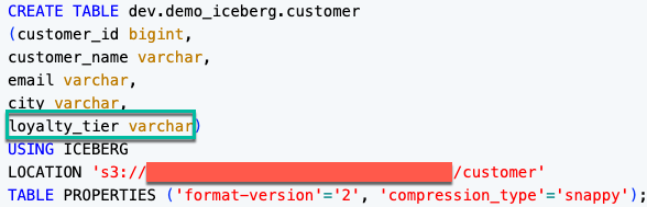
-- Add a loyalty_tier column to the customer table
ALTER TABLE dev.demo_iceberg.customer
ADD COLUMN loyalty_tier VARCHAR;

Verify the schema change:

SHOW TABLE dev.demo_iceberg.customer;
SHOW TABLE output showing the new loyalty_tier column added to the customer schema

Figure 3: SHOW TABLE output showing the loyalty_tier column added to the schema

The following output shows the new loyalty_tier column as NULL for existing rows:
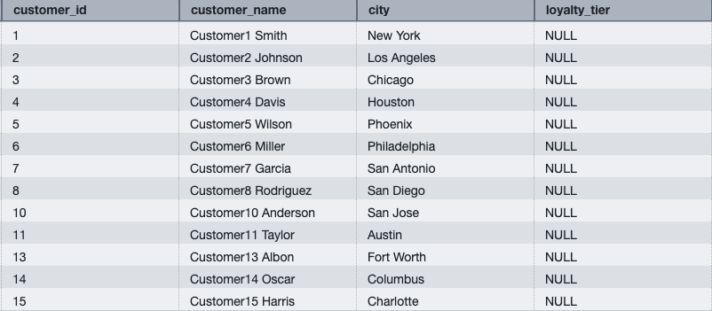
SELECT customer_id, customer_name, city, loyalty_tier
FROM dev.demo_iceberg.customer
ORDER BY customer_id;
Query results showing loyalty_tier as NULL for existing customer rows

Figure 4: Query results showing loyalty_tier as NULL for existing rows

Populate the new column by aggregating order totals from the orders table in S3 Tables:

-- Set loyalty_tier based on total spend from orders
UPDATE dev.demo_iceberg.customer
SET loyalty_tier = CASE
WHEN a.total_spend > 300 THEN 'Gold'
ELSE 'Silver'
END
FROM (
SELECT customer_id, SUM(total_order_amt) AS total_spend
FROM "iceberg-write-blog@s3tablescatalog".iceberg_write_namespace.orders
GROUP BY customer_id
) AS a
WHERE dev.demo_iceberg.customer.customer_id = a.customer_id;

The following output shows customer loyalty tiers after the update:
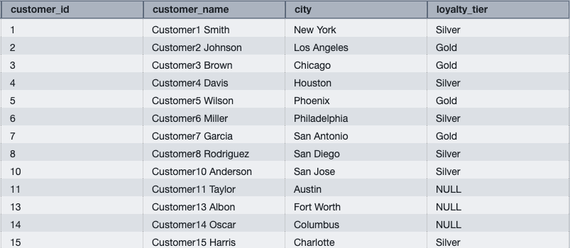
SELECT customer_id, customer_name, loyalty_tier
FROM dev.demo_iceberg.customer
ORDER BY customer_id;
Customer table query results showing Gold and Silver loyalty tiers

Figure 5: Customer table showing Gold and Silver loyalty tiers

Note: Customer IDs 11, 13, and 15 show NULL for loyalty_tier because they have no matching orders in the orders table.

Drop a column

Remove columns that are no longer needed. The column is removed from the current schema, but data in existing files remains untouched and simply becomes invisible to queries.

Verify the current schema:
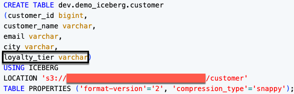
SHOW TABLE dev.demo_iceberg.customer;
SHOW TABLE output showing the customer schema before dropping loyalty_tier

Figure 6: SHOW TABLE output showing the current customer table schema before dropping loyalty_tier

Drop the column:

-- Drop the loyalty_tier column
ALTER TABLE dev.demo_iceberg.customer
DROP COLUMN loyalty_tier;

Verify the schema change:

SHOW TABLE dev.demo_iceberg.customer;
SHOW TABLE output showing the customer schema after loyalty_tier is dropped

Figure 7: SHOW TABLE output showing the customer table schema after loyalty_tier is dropped

Verify the column is dropped:
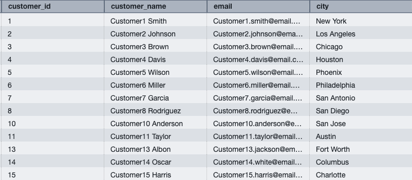
SELECT * FROM dev.demo_iceberg.customer
ORDER BY customer_id;
Query results confirming the loyalty_tier column no longer appears

Figure 8: Query results confirming the loyalty_tier column has been dropped

Note: To drop a column used in the current partition spec, first drop or replace the partition field, then drop the column.

Rename a column

Rename a column without affecting data types or partition specs:

-- Rename city to location
ALTER TABLE dev.demo_iceberg.customer
RENAME COLUMN city TO location;

The following output confirms the column has been renamed to location:
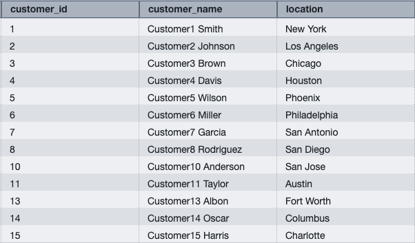
SELECT customer_id, customer_name, location
FROM dev.demo_iceberg.customer
ORDER BY customer_id;
Query results showing the city column renamed to location

Figure 9: Query results showing the renamed column location

Widen a column type

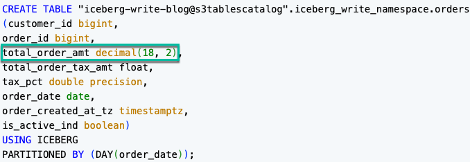
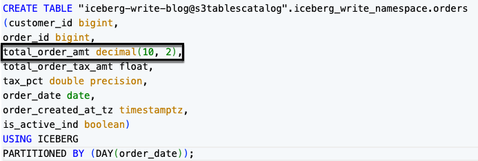
Widen a column’s data type without rewriting data. This is useful when your data outgrows the original precision, for example when order amounts exceed the original decimal range.

Verify the current column type:
SHOW TABLE "iceberg-write-blog@s3tablescatalog".iceberg_write_namespace.orders;
SHOW TABLE output showing total_order_amt as DECIMAL(10,2)

Figure 10: SHOW TABLE output showing total_order_amt as DECIMAL(10,2)

Now run the ALTER to widen the column:

-- Widen total_order_amt to support larger order values
ALTER TABLE "iceberg-write-blog@s3tablescatalog".iceberg_write_namespace.orders
ALTER COLUMN total_order_amt TYPE DECIMAL(18,2);

Verify the updated column type:

SHOW TABLE "iceberg-write-blog@s3tablescatalog".iceberg_write_namespace.orders;
SHOW TABLE output showing total_order_amt widened to DECIMAL(18,2)

Figure 11: SHOW TABLE output confirming total_order_amt widened to DECIMAL(18,2)

Note: Amazon Redshift supports safe type promotions (for example, INT to BIGINT, FLOAT to DOUBLE, DECIMAL(10,2) to DECIMAL(18,2)). Plan column types accordingly for future growth.

Set table properties

Change the compression type for future writes:

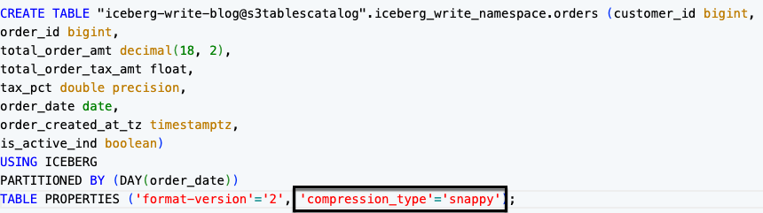
Verify the current compression type:
SHOW TABLE "iceberg-write-blog@s3tablescatalog".iceberg_write_namespace.orders;
SHOW TABLE output showing the orders table compression type before the change

Figure 12: SHOW TABLE output showing the current compression type before the update

Now run the ALTER to change the compression type:

-- Switch to zstd compression for better ratios
ALTER TABLE "iceberg-write-blog@s3tablescatalog".iceberg_write_namespace.orders
SET TABLE PROPERTIES ('compression_type'='zstd');

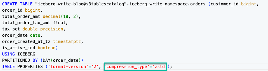
The following SHOW TABLE output confirms the updated compression setting:
SHOW TABLE "iceberg-write-blog@s3tablescatalog".iceberg_write_namespace.orders;
SHOW TABLE output showing compression_type set to zstd

Figure 13: SHOW TABLE output showing compression_type set to zstd

Note: This affects only future writes. Existing data files retain their original compression.

Partition evolution

A powerful feature of Iceberg is partition evolution, the ability to change how a table is partitioned without rewriting existing data. Amazon Redshift writes new data with the updated partition scheme, while existing data remains in the old layout. Query engines handle both layouts transparently.

Adding a partition field

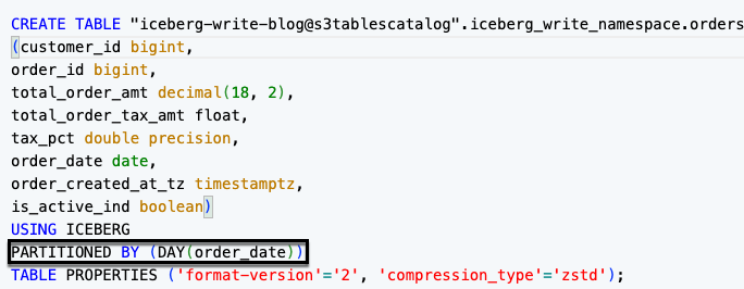
The orders table from Part 1 is partitioned by DAY(order_date). Add an additional bucket partition to distribute data across hash buckets:

Verify the current partition spec:
SHOW TABLE "iceberg-write-blog@s3tablescatalog".iceberg_write_namespace.orders;
SHOW TABLE output showing the orders partition spec before adding a field

Figure 14: SHOW TABLE output showing the current partition spec before adding a partition field

Add the partition field:

-- Add bucket partitioning on customer_id
ALTER TABLE "iceberg-write-blog@s3tablescatalog".iceberg_write_namespace.orders
ADD PARTITION FIELD bucket(16, customer_id);

After this change, new data is partitioned by both DAY(order_date) and bucket(16, customer_id), while existing data remains in the original day-only layout.

Verify the updated spec:
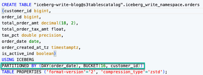
SHOW TABLE "iceberg-write-blog@s3tablescatalog".iceberg_write_namespace.orders;
SHOW TABLE output showing partition spec with DAY(order_date) and bucket(16, customer_id)

Figure 15: SHOW TABLE output showing the updated partition spec with DAY(order_date) and bucket(16, customer_id)

Replacing a partition field

Instead of separately dropping and adding, use REPLACE PARTITION FIELD as a single atomic operation. This is the recommended approach when swapping one transform for another on the same source column, because it makes the intent explicit and avoids a transient state where the table is unpartitioned between operations.

Verify the current partition spec:
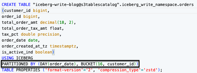
SHOW TABLE "iceberg-write-blog@s3tablescatalog".iceberg_write_namespace.orders;
SHOW TABLE output showing the current DAY(order_date) partition spec

Figure 16: SHOW TABLE output showing the current partition spec with DAY(order_date) and bucket(16, customer_id)

Replace the partition field:

-- Replace daily partitioning with monthly
ALTER TABLE "iceberg-write-blog@s3tablescatalog".iceberg_write_namespace.orders
REPLACE PARTITION FIELD DAY(order_date) WITH MONTH(order_date);

After this change:

  • Existing data remains in day-based partition folders.
  • Amazon Redshift writes new data into month-based partition folders.
  • The query engine reads both layouts transparently.

Confirm the new partition spec:
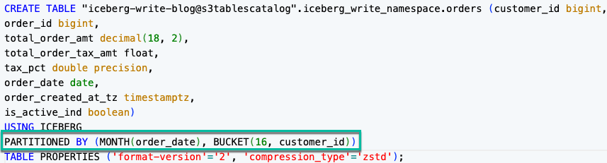
SHOW TABLE "iceberg-write-blog@s3tablescatalog".iceberg_write_namespace.orders;
SHOW TABLE output confirming the partition field replaced with MONTH(order_date)

Figure 17: SHOW TABLE output confirming the partition field replaced with MONTH(order_date)

Insert new data and verify that both partition layouts are queryable:
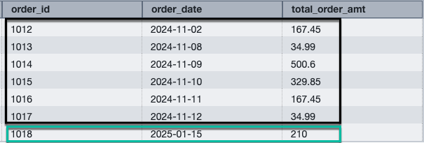
-- New data follows monthly partitioning
INSERT INTO "iceberg-write-blog@s3tablescatalog".iceberg_write_namespace.orders
(order_date, order_id, customer_id, total_order_amt, total_order_tax_amt,
tax_pct, order_created_at_tz, is_active_ind)
VALUES
('2025-01-15', 1018, 3, 210.00, 16.80, 0.08, '2025-01-15 09:00:00-06:00', true);
-- Query spans both old (daily) and new (monthly) layouts transparently
SELECT order_id, order_date, total_order_amt
FROM "iceberg-write-blog@s3tablescatalog".iceberg_write_namespace.orders
WHERE order_date >= '2024-11-01'
ORDER BY order_date;
Query results spanning both the daily and monthly partition layouts

Figure 18: Query results spanning both partition layouts

Converting to a multi-level partition

Iceberg supports multi-level (composite) partition specs, where data is organized by more than one partition field. You can evolve an existing single-level spec into a multi-level spec by adding partition fields one at a time. Each ADD PARTITION FIELD is a lightweight metadata operation, and no data is rewritten.

The orders table is currently partitioned by MONTH(order_date) and bucket(16, customer_id). Add one more partition field to create a three-level spec:

Verify the current partition spec:
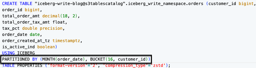
SHOW TABLE "iceberg-write-blog@s3tablescatalog".iceberg_write_namespace.orders;
SHOW TABLE output showing the two-level partition spec of MONTH(order_date) and bucket(16, customer_id)

Figure 19: SHOW TABLE output showing the current two-level partition spec of MONTH(order_date) and bucket(16, customer_id)

Add partition field to build the three-level spec:

-- Add a day-level partition field on order_created_at_tz
ALTER TABLE "iceberg-write-blog@s3tablescatalog".iceberg_write_namespace.orders
ADD PARTITION FIELD day(order_created_at_tz);

Verify the new multi-level partition spec:
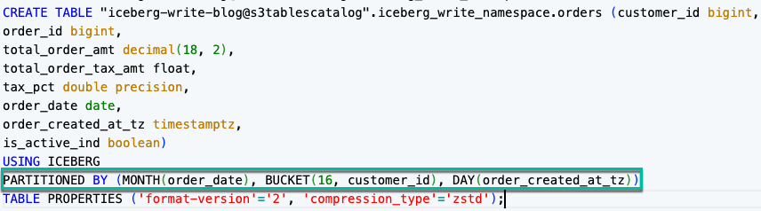
SHOW TABLE "iceberg-write-blog@s3tablescatalog".iceberg_write_namespace.orders;
SHOW TABLE output showing the three-level MONTH, bucket, and day partition spec

Figure 20: SHOW TABLE output showing the three-level partition spec of MONTH(order_date), bucket(16, customer_id), and day(order_created_at_tz)

After these changes:

  • Existing data remains in the original single-level layout (month-based folders).
  • Amazon Redshift writes new data into the multi-level layout (month, then bucket, then day folders).
  • The query engine reads both layouts transparently.

Dropping partition fields from a multi-level partition

You can also evolve in the other direction by removing partition fields from a multi-level spec to simplify the partition layout. Like adding fields, dropping a partition field is a metadata-only operation and removes one field per statement.

Verify the current multi-level partition spec:
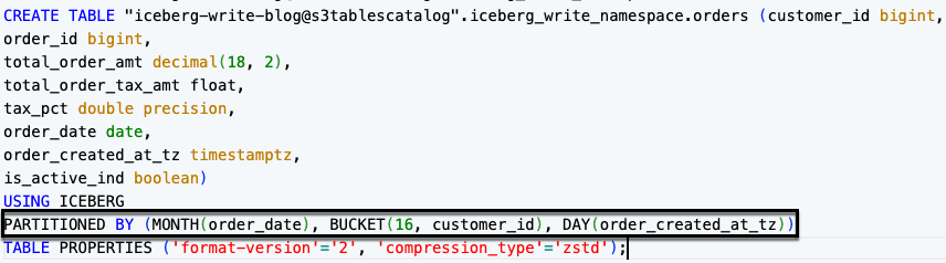
SHOW TABLE "iceberg-write-blog@s3tablescatalog".iceberg_write_namespace.orders;
SHOW TABLE output showing the three-level partition spec before dropping fields

Figure 21: SHOW TABLE output showing the three-level partition spec before dropping fields

Drop the partition fields one at a time:

-- Drop the bucket partition field
ALTER TABLE "iceberg-write-blog@s3tablescatalog".iceberg_write_namespace.orders
DROP PARTITION FIELD bucket(16, customer_id);
-- Drop the day-level partition field
ALTER TABLE "iceberg-write-blog@s3tablescatalog".iceberg_write_namespace.orders
DROP PARTITION FIELD day(order_created_at_tz);

Verify the table is back to its original single-level spec:
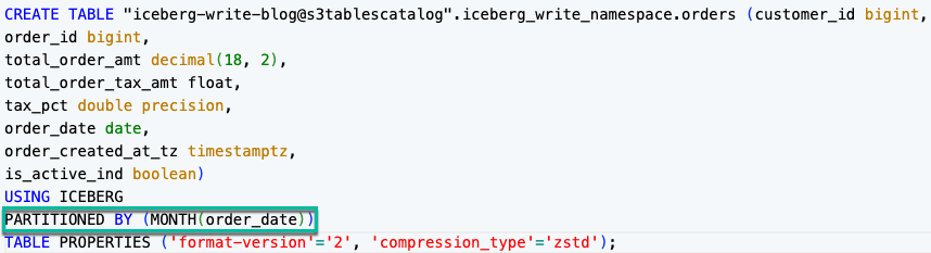
SHOW TABLE "iceberg-write-blog@s3tablescatalog".iceberg_write_namespace.orders;
SHOW TABLE output confirming the table back to a single-level MONTH(order_date) spec

Figure 22: SHOW TABLE output confirming the table is back to a single-level MONTH(order_date) partition spec

After dropping a partition field:

  • Data written under the dropped field’s layout stays in place and remains queryable.
  • Amazon Redshift writes new data using only the remaining partition fields.
  • Queries that filtered on the dropped field still work, but they no longer benefit from partition pruning on that field for newly written data.

Supported partition transforms

The following table lists the partition transforms available for Iceberg tables in Amazon Redshift:

Partition transform Syntax example What it does
Year year(order_date) Groups data into yearly partitions based on a date or timestamp column.
Month month(order_date) Groups data into monthly partitions based on a date or timestamp column.
Day day(order_date) Groups data into daily partitions based on a date or timestamp column.
Hour hour(event_ts) Groups data into hourly partitions based on a timestamp column.
Bucket bucket(16, customer_id) Distributes data across N hash buckets for even distribution on high-cardinality columns.
Truncate truncate(3, zip_code) Truncates column values to a fixed width W for grouping similar values together.
Identity identity(region) Partitions by the exact column value with no transformation applied.

Note: A column that is already part of an existing partition field can’t be used in a new partition field. Drop or replace the existing field first.

Accessing S3 Tables with external schemas

Lake Formation resource links provide cross-engine access to your S3 Tables through centralized governance. You create a resource link in the default AWS Glue Data Catalog that points to your S3 Tables database. Amazon Redshift, Amazon Athena, Amazon EMR, and other engines can then discover and query the tables using a single permission model.
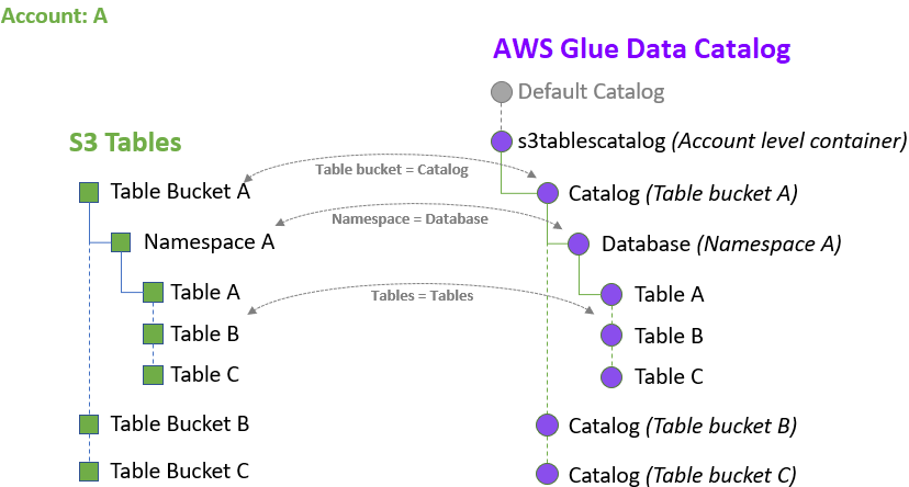
Diagram of S3 Tables integration with AWS Glue Data Catalog and Lake Formation

Figure 23: S3 Tables integration with AWS Glue Data Catalog and Lake Formation

For the complete setup walkthrough, including Lake Formation prerequisites, resource link creation, and permission grants, see Optimize Amazon S3 Tables queries with Amazon Redshift. For conceptual details on resource links and S3 Tables catalog integration, see About resource links and Creating an S3 Tables catalog.

The following steps show how to query S3 Tables through a resource link after completing the setup from the referenced blog.

In the Lake Formation console, the resource link appears as a database named iceberg_write_blog_rl (type: Resource link). To grant access to the resource link:

  1. In the Lake Formation console, choose Databases.
  2. Locate iceberg_write_blog_rl (type: Resource link).
  3. Choose Actions, then Grant.
  4. Grant DESCRIBE permission to RedshiftIcebergRole.

Create an external schema

With the resource link in place, create an external schema in Amazon Redshift for two-part notation access.

For IAM federated users:

CREATE EXTERNAL SCHEMA s3tables_iceberg
FROM DATA CATALOG
DATABASE 'iceberg_write_blog_rl'
CATALOG_ID '<ACCOUNT_ID>'
IAM_ROLE 'SESSION';

For database users and business intelligence (BI) tools:

CREATE EXTERNAL SCHEMA s3tables_iceberg
FROM DATA CATALOG
DATABASE 'iceberg_write_blog_rl'
IAM_ROLE 'arn:aws:iam::<ACCOUNT>:role/RedshifticebergRole';

Grant access to specific users or roles:
-- Grant to the IAM role used in this walkthrough
GRANT USAGE ON SCHEMA s3tables_iceberg TO "IAMR:RedshifticebergRole";
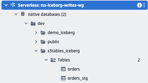
Amazon Redshift query showing S3 Tables available through the external schema

Figure 24: S3 Tables available through an external schema

Query with two-part notation

With the external schema created, query S3 Tables using two-part notation:
-- Instead of: "iceberg-write-blog@s3tablescatalog".iceberg_write_namespace.orders
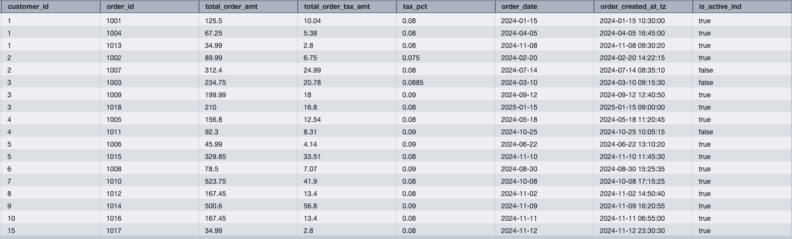
SELECT * FROM s3tables_iceberg.orders;
Query results from S3 Tables through the external schema using two-part notation

Figure 25: Query results from S3 Tables through an external schema using two-part notation

Access methods comparison

The following table compares the available methods for accessing Iceberg tables in Amazon Redshift:

Access method Query syntax Authentication Best for
S3 Tables three-part notation "bucket@s3tablescatalog".namespace.table IAM federated identity only Interactive queries in Query Editor v2 with direct catalog access.
External schema through resource link schema_name.table Any (IAM role defined in schema) BI tools, Data API, JDBC/ODBC applications, and shared team access.
awsdatacatalog awsdatacatalog.database.table IAM federated identity only Multi-database access in a single session without creating external schemas.

Bringing it together

Combine schema evolution with cross-engine access in a single workflow. The following example adds a column to the orders table and immediately queries it through the external schema:
-- 1. Add a column to the S3 Tables orders table
ALTER TABLE s3tables_iceberg.orders
ADD COLUMN fulfillment_status VARCHAR;
-- 2. Update the new column
UPDATE s3tables_iceberg.orders
SET fulfillment_status = 'shipped'
WHERE order_date < '2024-11-01';
UPDATE s3tables_iceberg.orders
SET fulfillment_status = 'pending'
WHERE order_date >= '2024-11-01';
-- 3. Query immediately via the external schema (no schema recreation needed)
SELECT o.order_id, o.order_date, o.fulfillment_status, c.customer_name
FROM s3tables_iceberg.orders o JOIN demo_iceberg.customer c
ON o.customer_id = c.customer_id
ORDER BY o.order_date DESC;
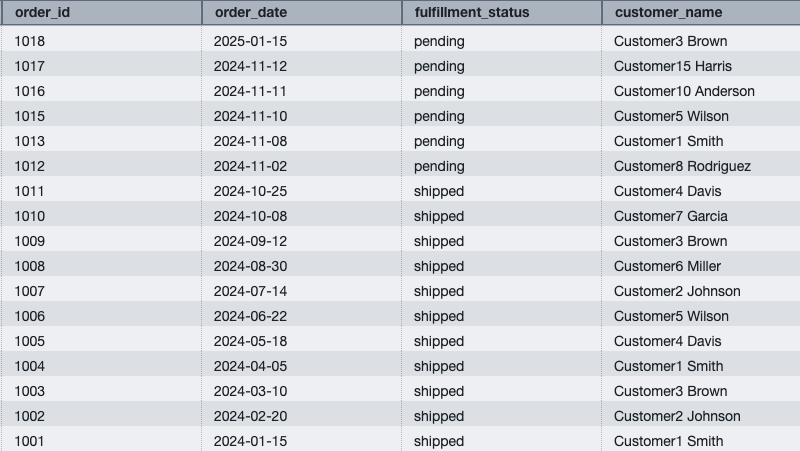
Query results of a cross-catalog join showing the evolved schema through the external schema

Figure 26: Cross-catalog join showing the evolved schema immediately visible through the external schema

The new column is visible through both the three-part notation and the external schema without any additional configuration, because the schema evolution in Iceberg propagates automatically.

Best practices

  • Test ALTER operations in non-production first. While metadata-only, schema changes affect all readers immediately.
  • Use REPLACE PARTITION FIELD instead of DROP + ADD. The atomic operation avoids a transient unpartitioned state.
  • Monitor partition spec changes with SHOW TABLE. Verify the current spec after any partition evolution.
  • Choose partition transforms based on query patterns. Use month() or day() for time-range filters. Use bucket() for high-cardinality join keys.
  • Set table properties before bulk loads. Change compression type (zstd for better ratios, snappy for speed) before large INSERT operations.
  • Run table maintenance after mutations. After performing multiple UPDATE, DELETE, or MERGE operations, run AWS Glue table optimizers to compact deletion files and improve read performance.
  • Use Lake Formation for fine-grained access. Column-level and row-level security can be applied through Lake Formation on tables accessed through resource links.
  • Grant schema access to specific users or roles. Avoid granting to PUBLIC. Use named IAM roles or database users for least-privilege access.
  • Monitor query performance. Use Amazon Redshift query monitoring features to track performance of write operations and optimize partitioning strategies as needed.

Considerations

Keep the following in mind when working with ALTER TABLE and partition evolution on Iceberg tables:

  • Plan for metadata-only behavior. ALTER TABLE operations update metadata instantly, and existing data files remain unchanged. All readers see the new schema immediately after the operation completes.
  • Drop partition fields before dropping partitioned columns. To remove a column used in the current partition spec, first drop or replace the partition field, then drop the column.
  • Use safe type promotions for ALTER COLUMN TYPE. Amazon Redshift supports widening within compatible families (INT to BIGINT, FLOAT to DOUBLE, DECIMAL(10,2) to DECIMAL(18,2)). Plan column types with future growth in mind.
  • Account for mixed partition layouts after evolution. Partition evolution doesn’t re-partition existing data. Old files remain in their original layout, and the query engine reads both layouts transparently.
  • Use external schemas for database user access. The auto-mounted three-part notation ("bucket@s3tablescatalog") requires IAM federated authentication. For database users and BI tools, create an external schema with an explicit IAM role.
  • Use full three-part notation with awsdatacatalog. The USE statement isn’t supported with awsdatacatalog, so always specify the full path.
  • Clean up S3 data separately after dropping tables. Dropping an Iceberg table removes only the catalog entry from AWS Glue Data Catalog. Delete the underlying S3 data files separately, or use AWS Glue table optimizers to remove orphaned files.

Clean up

To avoid ongoing charges, run the following:

-- Drop the fulfillment_status column added during testing
ALTER TABLE "iceberg-write-blog@s3tablescatalog".iceberg_write_namespace.orders
DROP COLUMN fulfillment_status;
-- Restore original partition spec (if changed)
ALTER TABLE "iceberg-write-blog@s3tablescatalog".iceberg_write_namespace.orders
REPLACE PARTITION FIELD MONTH(order_date) WITH DAY(order_date);
-- Drop external schema
DROP SCHEMA IF EXISTS s3tables_iceberg;

Conclusion

In this post, you evolved Apache Iceberg table schemas using ALTER TABLE operations. You added, dropped, and renamed columns, widened data types, changed compression, and evolved partition specs, all as metadata-only operations without rewriting data. You also created Lake Formation resource links to provide governed cross-engine access to S3 Tables, and simplified query syntax with external schemas.

This concludes the three-part series on getting started with Apache Iceberg write support in Amazon Redshift:

  1. Part 1: Create Iceberg tables and perform INSERT operations.
  2. Part 2: Run DELETE, UPDATE, and MERGE for row-level modifications.
  3. Part 3: Evolve schemas with ALTER TABLE and add cross-engine access with Lake Formation resource links.

If you have questions or feedback about this series, leave a comment on this post.

Additional resources


About the authors

Raghu Kuppala

Raghu Kuppala

Raghu is an Analytics Specialist Solutions Architect experienced working in the databases, data warehousing, and analytics space. Outside of work, he enjoys trying different cuisines and spending time with his family and friends.

Tanishq Goyal

Tanishq Goyal

Tanishq is a Software Development Engineer at AWS.

Sanket Hase

Sanket Hase

Sanket is an Engineering Manager with the Amazon Redshift team, leading query execution teams in the areas of data lake analytics, hardware-software co-design, and vectorized query execution.

Vlad Ponomarenko

Vlad Ponomarenko

Vlad is a Senior Software Development Engineer with the Amazon Redshift team, working on query processing, serverless, and integrations. Outside of work, he enjoys watching and playing sports and live music.

Sam Wang

Sam Wang

Sam works query processing and data ingestion as a Software Development Engineer on the Amazon Redshift team. When he’s not writing code, you’ll find him on the slopes.

Fahim Chodhury

Fahim Chowdhury

Fahim works on data lake query execution engine and query processing as a Software Development Engineer on the Amazon Redshift team.

Secure multi-warehouse Amazon Redshift access behind a Network Load Balancer using Microsoft Entra ID

Post Syndicated from Raghu Kuppala original https://aws.amazon.com/blogs/big-data/secure-multi-warehouse-amazon-redshift-access-behind-a-network-load-balancer-using-microsoft-entra-id/

As data analytics workloads scale, organizations face two challenges. First, they must deliver high-performance analytics at massive scale while maintaining secure access across diverse tools. Second, they must manage high-concurrency workloads while integrating with existing identity management systems.

You can address these challenges by using Amazon Redshift Serverless endpoints behind an AWS Network Load Balancer with Microsoft Entra ID federation. This architecture can authenticate while helping to streamline identity management across your data environment. Amazon Redshift Serverless provides petabyte-scale analytics with auto scaling capabilities, enabling high-concurrency workloads while streamlining user authentication and authorization.

In this post, we show you how to configure a native identity provider (IdP) federation for Amazon Redshift Serverless using Network Load Balancer. You will learn how to enable secure connections from tools like DBeaver and Power BI while maintaining your enterprise security standards.

Solution overview

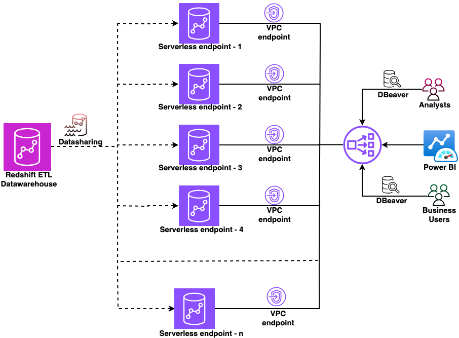
The following diagram shows the architecture.

Figure 1: Sample architecture diagram

Figure 1: Sample architecture diagram

In this architecture:

  • A central Amazon Redshift ETL data warehouse shares data to multiple Amazon Redshift Serverless workgroups using Amazon Redshift data sharing.
  • Each workgroup has a dedicated managed Amazon Virtual Private Cloud (Amazon VPC) endpoint.
  • A Network Load Balancer sits in front of all VPC endpoints, providing a single connection point.
  • Users connect from DBeaver or Power BI through the Network Load Balancer and authenticate using their Microsoft Entra ID credentials.

This setup works whether you’re validating the concept with a single workgroup today or planning to scale to multiple workgroups in the future.

Prerequisites

Before you begin, make sure that you have completed these prerequisites.

  1. Create Amazon Redshift Serverless endpoints.
  2. Set up datashare from producer to Amazon Redshift Serverless endpoints.
  3. Create Amazon Redshift-managed VPC endpoints.
  4. Create a Network Load Balancer.
  5. Configure a domain name.
  6. Set up Amazon Redshift native IdP federation with Microsoft Entra ID.
  7. Gather the following from your registered application in Microsoft Entra ID:
    1. Scope (API-Scope)
    2. Azure Client ID (AppID from App Registration Details)
    3. IdP Tenant (Tenant ID from App Registration Details)
  8. Download and install the latest Amazon Redshift JDBC and ODBC drivers.

This solution uses the following AWS services.

Implementation steps

This section covers configuring the Network Load Balancer, setting up an ACM certificate, creating custom domain names in Amazon Redshift, configuring DNS records in Amazon Route 53, and connecting your JDBC and ODBC clients using Microsoft Entra ID authentication.

1. Configure the Network Load Balancer

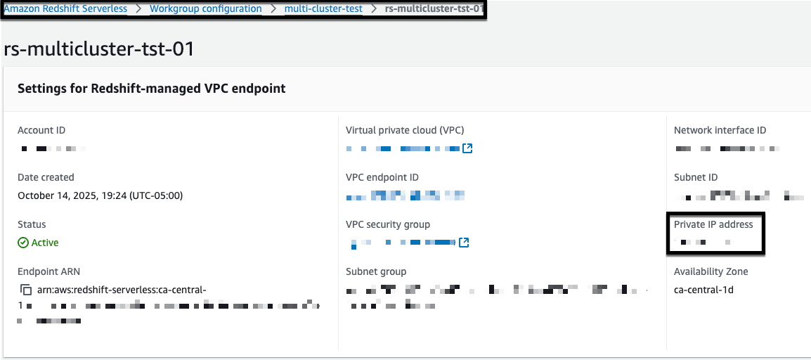
First, collect the private IP addresses for your Amazon Redshift-managed VPC endpoints:

  1. Open the Amazon Redshift Serverless console.
  2. Choose your workgroup.
  3. Note the private IP address of your Redshift-managed VPC endpoint.
  4. Repeat for each Amazon Redshift Serverless endpoint that you want to add to the Network Load Balancer.

    Figure 2: Amazon Redshift managed VPC endpoint

    Figure 2: Amazon Redshift managed VPC endpoint

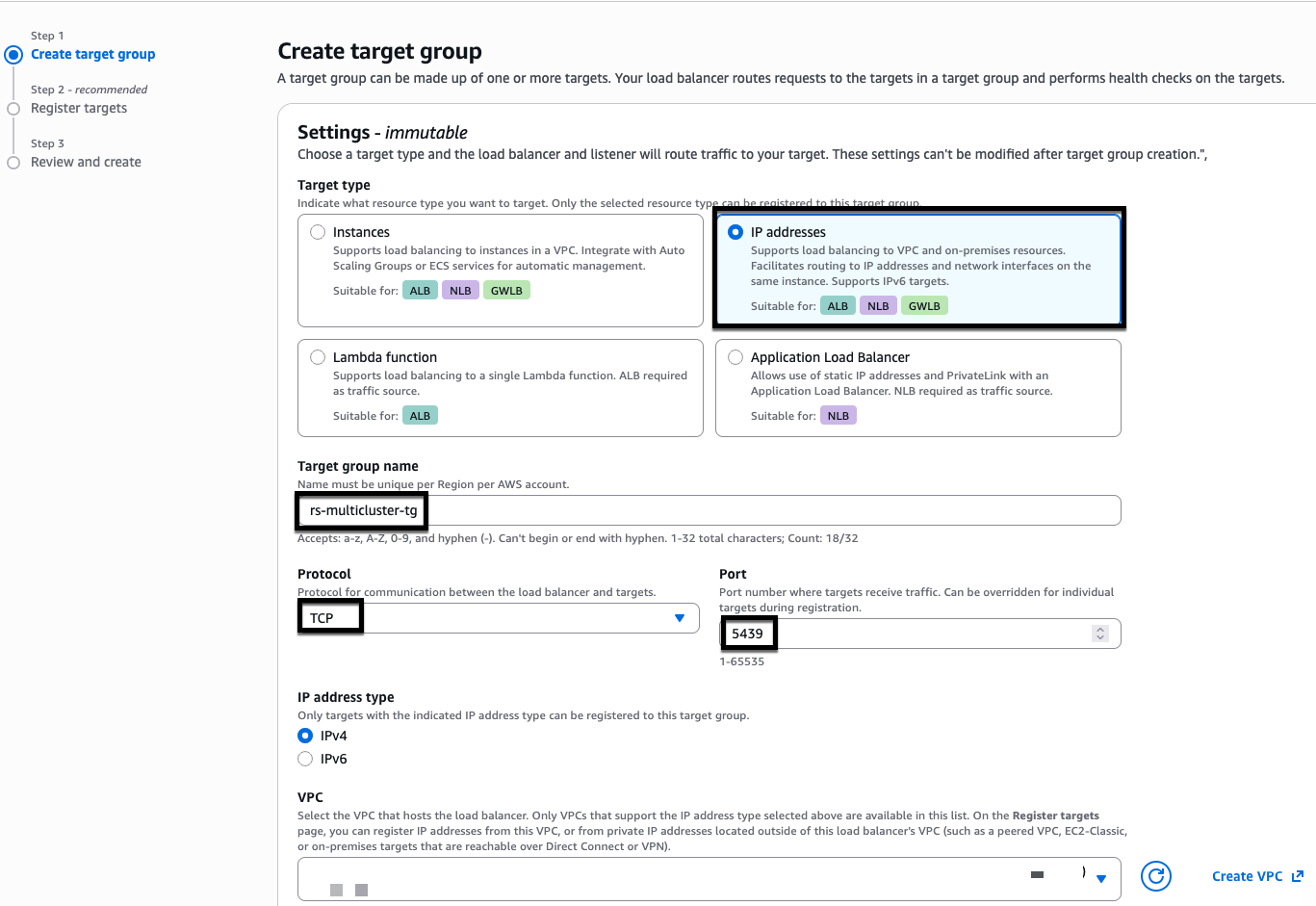
Next, create a target group for your endpoints:

  1. Open the Amazon Elastic Compute Cloud (Amazon EC2) console.
  2. Choose Target Groups.
  3. Choose Create target group.
  4. Configure the target group:
    • For Target type, choose IP addresses.
    • For Target group name, enter rs-multicluster-tg.
    • For Protocol, choose TCP.
    • For Port, enter 5439 (Note: You can find your specific port number in the Redshift endpoint connection details. If you haven’t modified it, use the default port 5439.).
    • For VPC, select your VPC.
    • Choose Next.
    Figure 3: create target group in NLB

    Figure 3: create target group in NLB

    Figure 4: NLB target group creation

    Figure 4: NLB target group creation

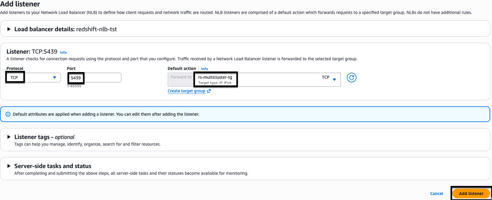
Add a listener to your Network Load Balancer:

  1. In the EC2 console, choose Load Balancers.
  2. Select your Network Load Balancer.
  3. In the Listeners tab, choose Add listener.
  4. Configure the listener:
    • For Protocol, choose TCP.
    • For Port, enter 5439.
    • For Default action, choose rs-multicluster-tg.
  5. Choose Add listener.

    Figure 5: NLB listener properties.

    Figure 5: NLB listener properties.

2. Configure AWS Certificate Manager (ACM)

For this example, we use myexampledomain.com as a custom domain. Replace it with your own domain name before you begin.Follow these steps to request and configure your certificate:

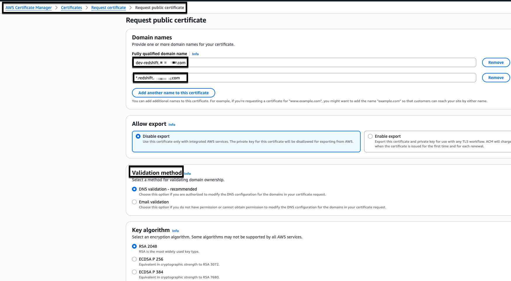
  1. Request a certificate in AWS Certificate Manager (ACM):
    • Open the AWS Certificate Manager console.
    • Choose Request Certificate.
    • Choose Request Public certificate.
    • Choose Next.
  2. Configure the certificate:
    • Add two domain names:
      • Network Load Balancer CNAME: dev-redshift.myexampledomain.com
      • Wildcard domain: *.redshift.myexampledomain.com
    • For Validation method, choose DNS validation.
    • Choose Request.

    For enhanced security, we recommend adding individual Amazon Redshift Serverless CNAMEs instead of using wildcards (*). This example uses DNS validation in AWS Certificate Manager, which requires creating CNAME records to prove domain control.

    Figure 6: AWS Certificate Manager (ACM) certificate creation

    Figure 6: AWS Certificate Manager (ACM) certificate creation

  3. Validate the certificate:
    • Your AWS Certificate Manager (ACM) certificate initially shows a ‘Pending validation’ status.
    • Wait for the status to change to ‘Issued’ before proceeding.
    • You must have an ‘Issued’ status before creating Amazon Redshift custom domain names.
    Figure 7: Sample issued AWS Certificate Manager (ACM) certificate

    Figure 7: Sample issued AWS Certificate Manager (ACM) certificate

3. Configure Amazon Redshift custom domain names

  1. Create a custom domain name:
    • Open the Amazon Redshift Serverless console.
    • Select your workgroup.
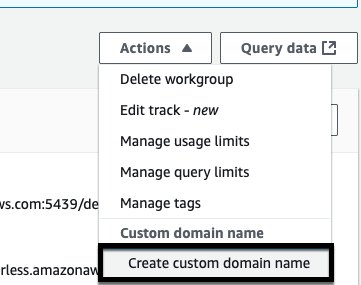
    • From Actions, choose Create custom domain name.
    Figure 8: Amazon Redshift custom domain name creation

    Figure 8: Amazon Redshift custom domain name creation

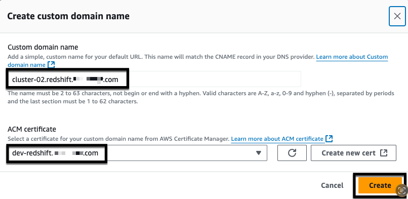
  2. Configure the domain settings:
    • For Custom domain name, enter cluster-02.redshift.myexampledomain.com.
    • For ACM certificate, select the certificate you created for dev-redshift.myexampledomain.com.
    • Choose Create.
    Figure 9: Amazon Redshift custom domain name creation

    Figure 9: Amazon Redshift custom domain name creation

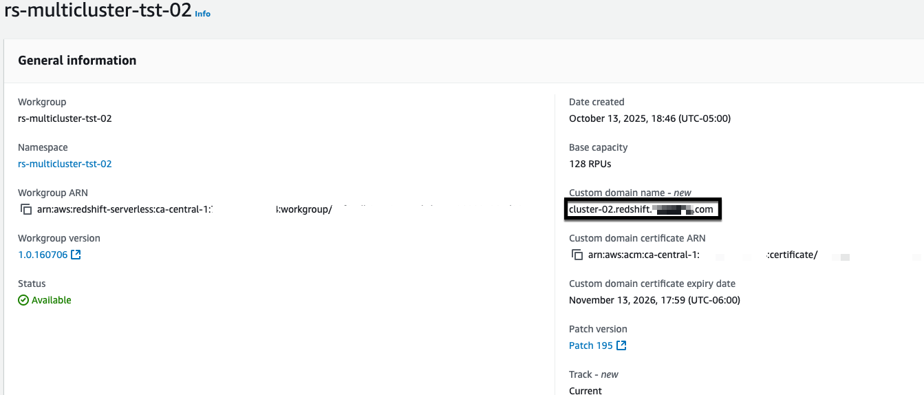
  3. Verify that the custom domain name appears in your workgroup.

    Figure 10: Amazon Redshift custom domain name

    Figure 10: Amazon Redshift custom domain name

  4. Repeat steps 1–3 for each remaining Amazon Redshift Serverless endpoint that you want to add to the Network Load Balancer. Use a unique custom domain name for each endpoint (for example, cluster-03.redshift.myexampledomain.com, cluster-04.redshift.myexampledomain.com) and select the same ACM certificate that you created earlier.

4. Configure Amazon Route 53

Amazon Route 53 maps your custom domain name to the correct Amazon Redshift endpoint, making it reachable by name rather than a system-generated address. Without it, clients have no way to resolve your custom domain and AWS Certificate Manager can’t verify domain ownership to enable secure connections.First, create a CNAME record for your Network Load Balancer:

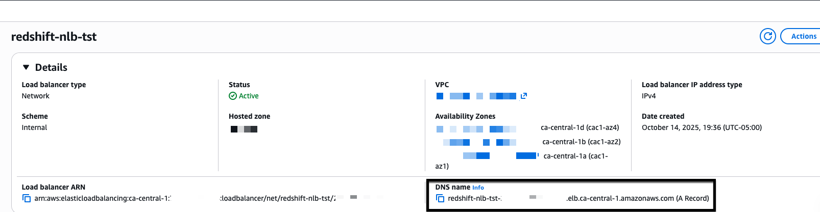
  1. Get the Network Load Balancer DNS name:
    • Open the Amazon EC2 console.
    • Choose Load Balancers.
    • Select your Network Load Balancer.
    • Copy the DNS name.
    Figure 11: NLB DNS name

    Figure 11: NLB DNS name

  2. Create Route 53 records:
    • Open the Amazon Route 53 console.
    • Choose Hosted Zones.
    • Select myexampledomain.com.
    • Choose Create record.
    • Configure the record:
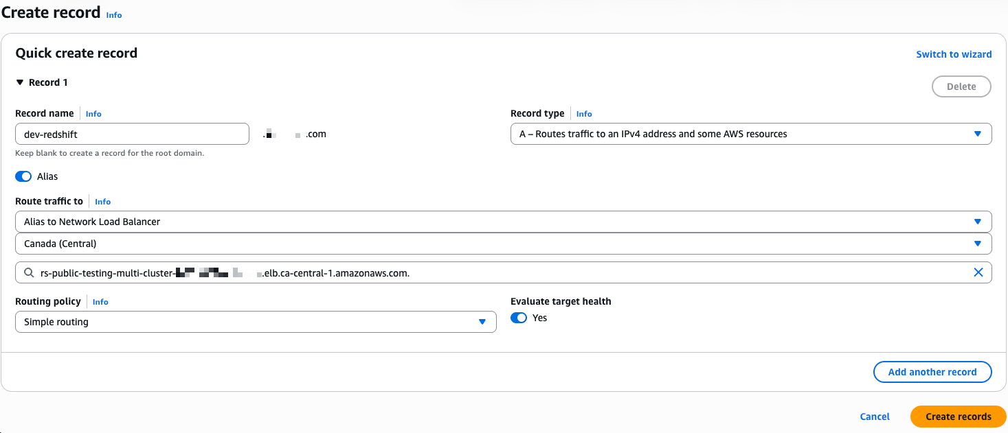
      • For Record name, enter dev-redshift.myexampledomain.com.
      • For Record type, choose A – Routes traffic to an IPv4 address and some AWS resources.
      • For Alias, choose Yes.
      • For Route traffic to, choose Alias to Network Load Balancer.
      • Select your AWS Region and Network Load Balancer DNS name.
      • For Routing policy, choose Simple routing.
      • Choose Create records.
    Figure 12: NLB - A record in route 53

    Figure 12: NLB – A record in route 53

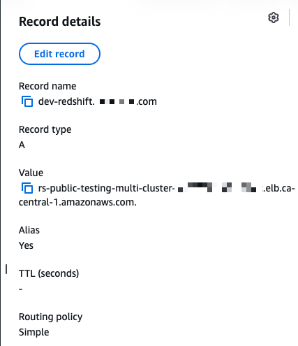
    Figure 13: NLB - A record in Route 53

    Figure 13: NLB – A record in Route 53

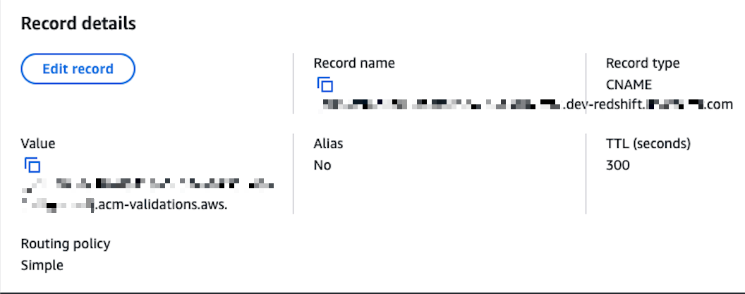
  3. Create the AWS Certificate Manager (ACM) validation CNAME:
    • Open AWS Certificate Manager.
    • Select your certificate for dev-redshift.myexampledomain.com.
    • Copy the CNAME name and CNAME value.
    • Return to Route 53.
    • Create a CNAME record in your myexampledomain.com hosted zone using the values from AWS Certificate Manager (ACM).
    • Choose Create records.
    Figure 14: NLB – CNAME record in Route 53

    Figure 14: NLB – CNAME record in Route 53

5. Configure Amazon Redshift JDBC and ODBC drivers with native IdP

The JDBC and ODBC driver configuration connects your client applications to Amazon Redshift through the Network Load Balancer using your Microsoft Entra ID credentials for authentication. Configuring both drivers allows any tool, whether DBeaver using JDBC or Power BI using ODBC, to authenticate through the same identity provider and reach the correct Amazon Redshift endpoint through a single connection point.

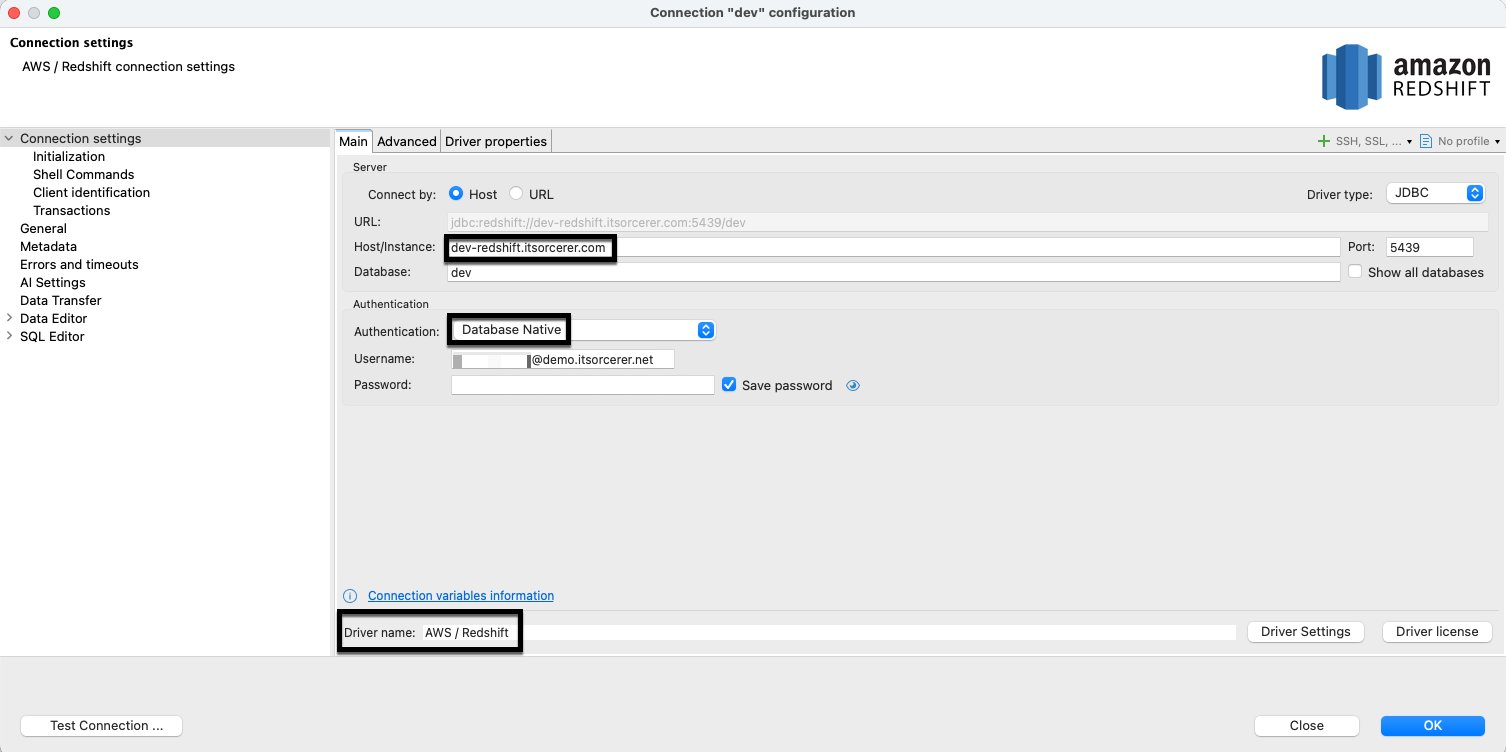
JDBC driver setup in DBeaver

  1. Create a new Amazon Redshift connection:
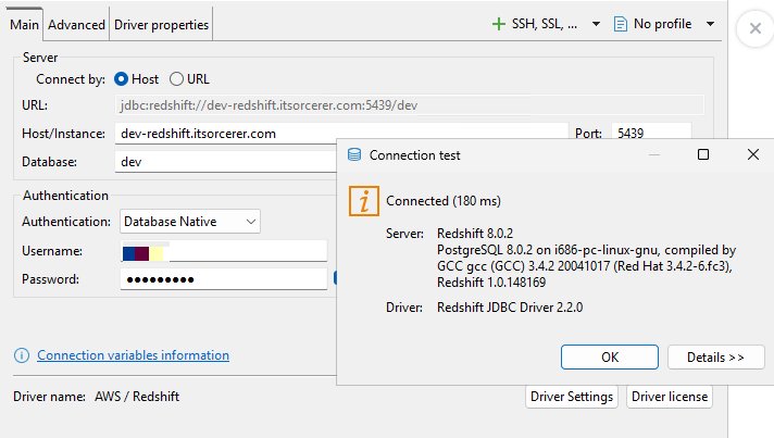
    • Host: dev-redshift.myexampledomain.com (NLB CNAME).
    • Database: dev.
    • Authentication: Database Native.
    • Username: login id for a user account.
    Figure 15: Amazon Redshift JDBC driver setup

    Figure 15: Amazon Redshift JDBC driver setup

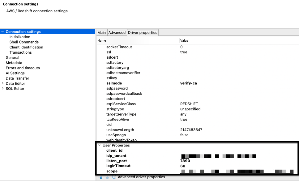
  2. Configure driver properties:
    • plugin_name: com.amazon.redshift.plugin.BrowserAzureOAuth2CredentialsProvider.
    • sslmode: verify-ca.
  3. Add user driver properties:
    • client_id: [Your Microsoft Entra ID application client ID].
    • idp_tenant: [Your Microsoft Entra ID tenant].
    • listen_port: 7890.
    • loginTimeout: 60.
    • scope: [Your Microsoft Entra ID application scope].
    Figure 16: Amazon Redshift JDBC driver user properties

    Figure 16: Amazon Redshift JDBC driver user properties

ODBC driver setup

  1. Configure the system DSN:
    • Open ODBC Data Source Administrator (64-bit).
    • Choose System DSN.
    • Choose Add.
    • Select Amazon Redshift ODBC Driver (x64) 2.01.04.00.
    • Choose Finish.
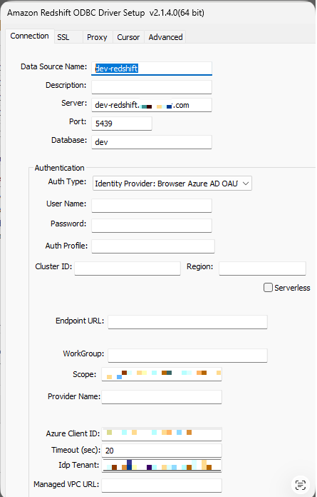
  2. Configure connection settings:
    • Data Source Name: dev-redshift.
    • Server: dev-redshift.myexampledomain.com.
    • Port: 5439.
    • Database: dev.
    • Auth type: Identity Provider: Browser Azure AD OAUTH2.
    • Scope: [Your Microsoft Entra ID application scope].
    • Azure Client ID: [Your Microsoft Entra ID application client ID].
    • IdP Tenant: [Your Microsoft Entra ID application tenant].
    Figure 17: Amazon Redshift ODBC driver properties

    Figure 17: Amazon Redshift ODBC driver properties

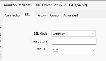
  3. Configure SSL settings:
    • SSL Mode: verify-ca.
    • Choose Save.
    Figure 18: Amazon Redshift ODBC driver properties

    Figure 18: Amazon Redshift ODBC driver properties

6. Validate connectivity

Test DBeaver connection

  1. After configuring the JDBC driver properties, choose Test Connection.
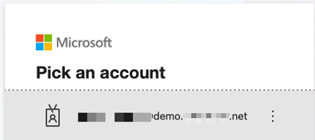
  2. Authenticate through the Microsoft login in your browser.
  3. Verify that you receive a success message.
  4. Confirm successful connection using Native IdP through the Network Load Balancer.
Figure 19: Microsoft Entra id authentication

Figure 19: Microsoft Entra id authentication

Figure 20: Successful Microsoft Entra id authentication

Figure 20: Successful Microsoft Entra id authentication

Figure 21: Successful Amazon Redshift authentication

Figure 21: Successful Amazon Redshift authentication

Test power BI desktop connection

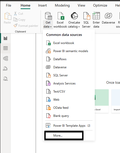
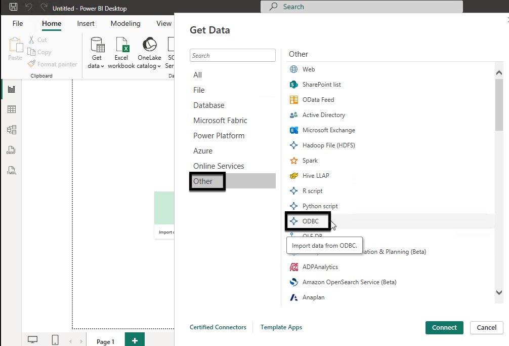
  1. Launch Power BI Desktop:
    • Choose Get data.
    • Choose More.
    • Under Other, select ODBC.
    • Choose Connect.
    Figure 22: Power BI desktop connectivity using Amazon Redshift ODBC driver

    Figure 22: Power BI desktop connectivity using Amazon Redshift ODBC driver

    Figure 23: Power BI desktop connectivity using Amazon Redshift ODBC driver

    Figure 23: Power BI desktop connectivity using Amazon Redshift ODBC driver

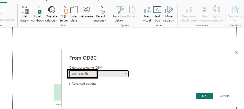
  2. Configure the connection:
    • Select dev-redshift from the Data source name.
    • Choose OK.
    • Complete Microsoft Entra ID authentication in your browser.
    Figure 24: Power bi desktop connectivity using Amazon Redshift odbc driver

    Figure 24: Power bi desktop connectivity using Amazon Redshift odbc driver

    Figure 25: Successful Microsoft Entra id authentication

    Figure 25: Successful Microsoft Entra id authentication

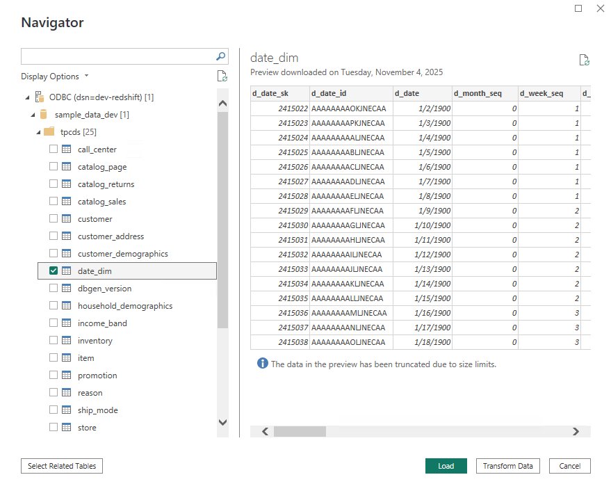
  3. Test the connection:
    • From Navigator, choose schema tpcds.
    • Select date_dim.
    • Choose Load.
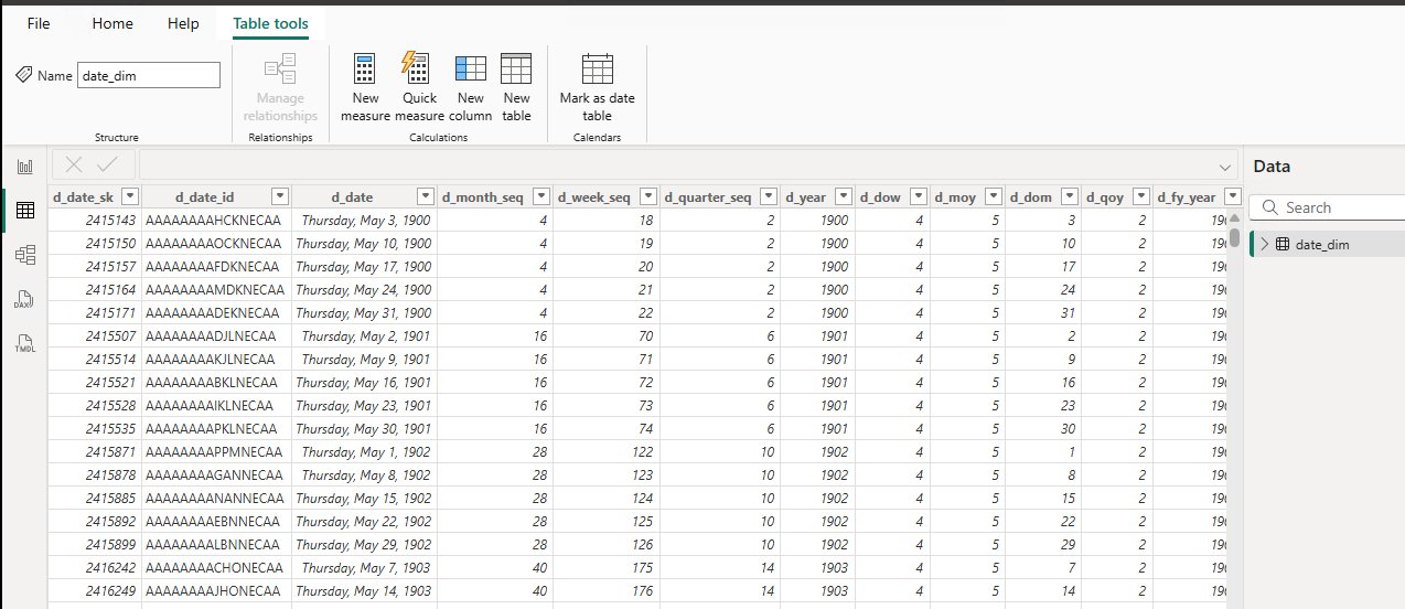
    • Verify that you can analyze your Amazon Redshift data in Power BI Desktop.
    Figure26: Power BI desktop connected to Amazon Redshift and schema browsing

    Figure26: Power BI desktop connected to Amazon Redshift and schema browsing

    Figure 27: Power BI desktop fetching data from date_dim table

    Figure 27: Power BI desktop fetching data from date_dim table

Cleaning up

To avoid ongoing charges, delete the following resources:

  1. Delete the Amazon Redshift data warehouses (provisioned cluster or serverless workgroup and namespace) and the VPC endpoints that you created.
  2. Delete the certificate that you created in AWS Certificate Manager (ACM).
  3. Delete the Network Load Balancer.

Conclusion

In this post, we showed you how to integrate Amazon Redshift Serverless with Microsoft Entra ID using an AWS Network Load Balancer as a single connection endpoint across multiple workgroups. As your data analytics use cases grow, you can continue to scale horizontally by adding new workgroups behind the same Network Load Balancer without changing your users’ connection settings or authentication experience.

For more information about extending and scaling this solution, see the following resources:

AWS Blogs


About the authors

Raghu Kuppala

Raghu Kuppala

Raghu is an Analytics Specialist Solutions Architect experienced working in the databases, data warehousing, and analytics space. Outside of work, he enjoys trying different cuisines and spending time with his family and friends.

Raza Hafeez

Raza Hafeez

Raza is a Senior Product Manager at Amazon Redshift. He has over 13 years of professional experience building and optimizing enterprise data warehouses and is passionate about enabling customers to realize the power of their data. He specializes in migrating enterprise data warehouses to AWS Modern Data Architecture.

Harshida Patel

Harshida Patel

Harshida is a Analytics Specialist Principal Solutions Architect, with AWS.

Justin Chin-You

Justin Chin-You

Justin is a Solutions Architect at AWS, working with Financial Services organizations. He is helping these organizations identify the right cloud transformation strategy based on industry trends and their organizational priorities.

Scale fine-grained permissions across warehouses with Amazon Redshift and AWS IAM Identity Center

Post Syndicated from Raghu Kuppala original https://aws.amazon.com/blogs/big-data/scale-fine-grained-permissions-across-warehouses-with-amazon-redshift-and-aws-iam-identity-center/

Amazon Redshift is a fully managed, petabyte-scale cloud-based data warehouse that you can use to scale analytics workloads effortlessly. As organizations expand their analytics capabilities across multiple business units, they need streamlined approaches for defining and managing fine-grained permissions for each warehouse. Many organizations use external identity providers (IdPs) like Microsoft Entra ID, Okta, or Ping to manage workforce identities centrally and need streamlined data warehouse integration with consistent access controls. We address these challenges by introducing Amazon Redshift federated permissions with AWS IAM Identity Center integration so that you can define security policies once and automatically enforce them across the warehouses in your account.

Amazon Redshift federated permissions are now supported with IAM Identity Center across multiple AWS Regions, where you can use identities from supported identity provider (IdP) such as Microsoft Entra ID, Okta, Ping Identity, or OneLogin across supported AWS Regions with IAM Identity Center. This enables you to align with business requirements including resiliency and proximity to users. You can now extend IAM Identity Center from your primary AWS Region to additional Regions of your choice based on your data residency requirements. In that region, you can get horizontal multi-warehouse scalability by adding new warehouses using Amazon Redshift federated permissions across multiple warehouses. With Redshift federated permissions, you define data permissions once from any Redshift warehouse in that region and automatically enforce them across all warehouses in the account in that region.

This post provides a comprehensive technical walkthrough for implementing Amazon Redshift federated permissions with AWS IAM Identity Center to help achieve scalable data governance across multiple data warehouses. It demonstrates a practical architecture where an Enterprise Data Warehouse (EDW) serves as the producer data warehouse with centralized policy definitions, helping automatically enforce security policies to consuming Sales and Marketing data warehouses without manual reconfiguration. You will learn how to do the following:

  • Configure IAM Identity Center connections for both data sharing producers and consumers
  • Register Amazon Redshift serverless namespaces with AWS Glue Data Catalog
  • Set up trusted identity propagation (TIP)
  • Create and attach Dynamic data masking policies to help protect personally identifiable information (PII) like customer dates of birth
  • Implement row-level security policies to control data visibility based on user roles
  • Map IdP groups to Amazon Redshift database roles for seamless access management

Prerequisites

Before you begin, verify that you have the following:

  • An AWS account with admin role privileges
  • Assign data lake admin permissions to above admin role. For instructions, see Create a data lake administrator
  • Enable IAM Identity Center integration using the Lake Formation
  • Review the blog post to understand the setup process of AWS IAM Identity Center integration with Amazon Redshift Query Editor v2
  • IAM Identity Center enabled in your AWS account, with users and groups created as listed under Solution overview section of User access (figure 2)
  • As an Amazon Redshift superuser, grant CONNECT, CREATE TABLE, INSERT, SELECT, and sys:secadmin permissions to AWSIDC:awssso-admin database role
  • An IAM role for IAM Identity Center access:
    • Step 1:Create an IAM policy for Amazon Redshift access. To integrate Amazon Redshift with IAM Identity Center, create an IAM policy (for example, aws-idc-policy) in the account where your Amazon Redshift data warehouse exists:
      {
        "Version": "2012-10-17",
        "Statement": [
          {
            "Sid": "VisualEditor0",
            "Effect": "Allow",
            "Action": [
              "redshift:DescribeQev2IdcApplications",
              "redshift-serverless:ListNamespaces",
              "redshift-serverless:ListWorkgroups",
              "redshift-serverless:GetWorkgroup"
            ],
            "Resource": [
              "arn:aws:redshift-serverless:<AWS Region>:<AWS Account ID>:workgroup/*",
              "arn:aws:redshift-serverless:<AWS Region>:<AWS Account ID>:namespace/*"
            ]
          },
          {
            "Sid": "VisualEditor1",
            "Effect": "Allow",
            "Action": [
              "sso:DescribeApplication",
              "sso:DescribeInstance"
            ],
            "Resource": [
              "arn:aws:sso:::instance/<IAM Identity Center Instance ID>",
              "arn:aws:sso::<AWS Account ID>:application/<IAM Identity Center Instance ID>/*"
            ]
          }
        ]
      }

    • Step 2: Create the IAM role. Create an IAM role (Amazon Redshift – Customizable) in the account where your Amazon Redshift data warehouse exists (for example, IAMIDCRedshiftRole).
    • Step 3: Attach IAM policies to the role. Attach the following two IAM policies to the previously mentioned role:
    • Step 4: Update the trust relationships. Update the trust relationships for this role with the following:
      {
        "Version": "2012-10-17",
        "Statement": [
          {
            "Effect": "Allow",
            "Principal": {
              "Service": "redshift.amazonaws.com"
            },
            "Action": [
              "sts:AssumeRole",
              "sts:SetContext"
            ]
          }
        ]
      }

      Note: AmazonRedshiftFederatedAuthorization is a managed policy that provides the necessary permissions for running queries with Amazon Redshift federated authorization.

  • Attach above IAMIDCRedshiftRole IAM role to all Redshift serverless endpoints

Solution overview

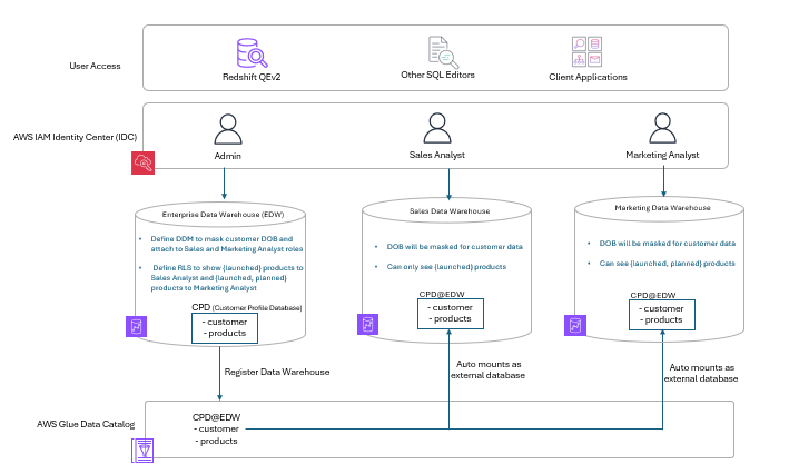
The following architecture diagram demonstrates federated permissions in a multi-warehouse environment, enabling scalable data governance across Amazon Redshift warehouses by automatically enforcing security policies.

Figure 1 : Sample architecture diagram

Figure 1: Sample architecture diagram

User access

Users can access data warehouses through Amazon Redshift Query Editor v2, third-party SQL editors (such as DBeaver and SQL Workbench), or custom client applications. The access methods help provide consistent security enforcement.

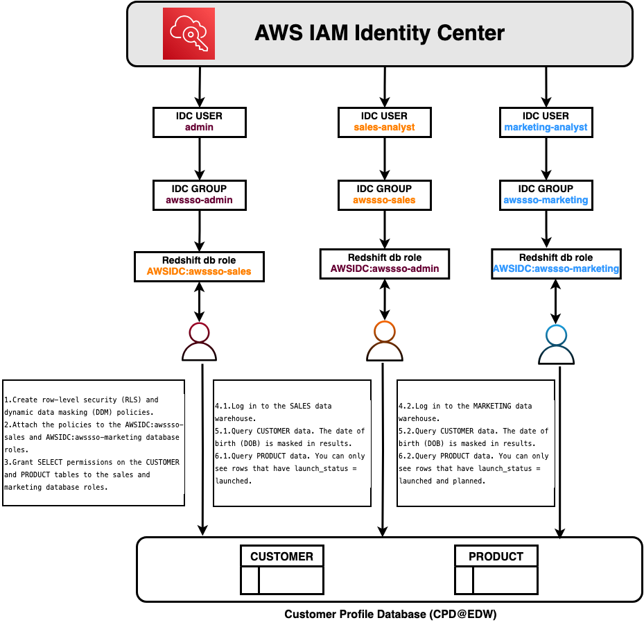
Figure 2: Solution overview flow

Figure 2: Solution overview flow

AWS IAM Identity Center integration

IAM Identity Center provides centralized authentication with single sign-on capabilities and automatically assigns role-based permissions based on organizational roles. This identity federation links corporate identities directly to AWS resources, making sure that authentication occurs at the identity layer before warehouse access.

Multi-warehouse architecture

This architecture uses three distinct data warehouses that serve different business functions while sharing centralized security policies.

Enterprise Data Warehouse (EDW)

The EDW serves as the central repository for enterprise data. In this architecture, customer and product data are stored in the Customer Profile Database (CPD), where administrators define two critical security policies:

  • Dynamic data masking (DDM) – Masks sensitive customer Date of Birth (DOB) fields for both Sales Analyst and Marketing Analyst roles, helping protect personally identifiable information (PII) while allowing analytical work
  • Row-level security (RLS) – Controls product visibility based on user roles. Sales Analysts view only launched products, while Marketing Analysts view both launched and planned products

The EDW registers with the AWS Glue Data Catalog, creating a unified metadata repository that makes data discoverable across the warehouses in the account. This registration establishes the foundation for federated permissions, enabling automatic policy propagation.

Sales data warehouse

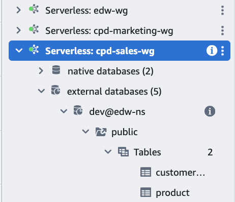
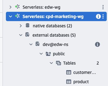
When Sales Analysts query customer and product tables, the system automatically enforces policies defined in the EDW through federated permissions. The registered namespace from the EDW automatically mounts as an external database, alleviating the need to recreate or reattach policies. Customer DOB fields appear masked, and only launched products are visible without additional configurations.

Marketing data warehouse

The Marketing Data Warehouse automatically inherits and enforces EDW security policies. Customer DOB fields remain masked to help protect PII, but with RLS policies, Marketing Analysts can view both launched and planned products. This provides the broader visibility needed for marketing planning. This differentiated access control is automatically enforced based on user roles.

Walkthrough

In this walkthrough, you create two Amazon Redshift IAM Identity Center (IDC) connections:

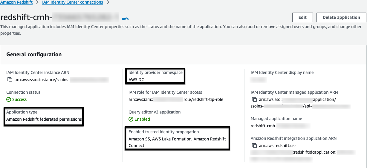
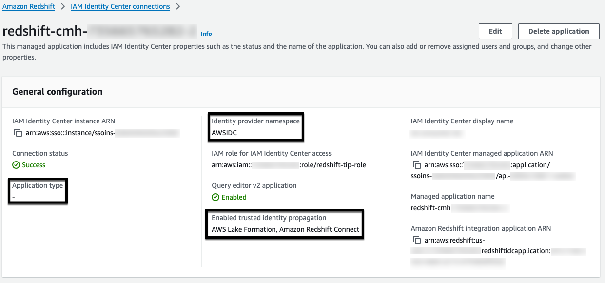
  1. Data sharing producer identity center connection – Assigned to the edw-wg Amazon Redshift serverless workgroup
  2. Data sharing consumer identity center connection – Assigned to the cpd-sales-wg and cpd-marketing-wg Amazon Redshift serverless workgroups

Set up IDC connections for Amazon Redshift federated permissions

In this section, you configure the IAM Identity Center connections that enable federated authentication across your warehouses. You will create separate connections for the producer (policy-defining) warehouse and consumer warehouses.

Configure Amazon Redshift data sharing producer IDC connection

To create the producer IDC connection:

  1. Open the Amazon Redshift Serverless console.
  2. Choose IAM Identity Center connections by expanding the hamburger menu.
  3. Choose Create application.
  4. Verify that you see “Amazon Redshift connected to IAM Identity Center”, and then choose Next.
  5. Configure the connection properties:
    • For IAM Identity Center display name, enter a name.
    • For Managed application name, enter rs-multicluster-producer.
    • For Identity provider namespace, choose AWSIDC.
    • For IAM role for IAM Identity Center access, choose the TIP IAM role that you created.
    • For Query editor v2 application, choose Enable the query editor v2 application.
    • For IAM Identity Center application type, choose Configure Amazon Redshift federated permissions using AWS IAM Identity Center (Recommended).
    • Choose Next.
  6. For Configure client connections that use third-party IdPs, choose No.
  7. Choose Next.
  8. Verify that the configuration details match your inputs and then choose Create Application.
Figure 3: Data sharing producer IDC connection

Figure 3: Data sharing producer IDC connection

Configure data sharing consumer IDC connection

To create the consumer IDC connection:

  1. Open the Amazon Redshift Serverless console.
  2. Choose IAM Identity Center connections by expanding the hamburger menu.
  3. Choose Create application.
  4. Verify that you see “Amazon Redshift connected to IAM Identity Center”, and then choose Next.
  5. Configure the connection properties:
    • For IAM Identity Center display name, enter a name.
    • For Managed application name, enter rs-multicluster-consumer.
    • For Identity provider namespace, choose AWSIDC.
    • For IAM role for IAM Identity Center access, choose the TIP IAM role that you created.
    • For Query editor v2 application, you will see the notification “You already have a query editor v2 application.”
    • For IAM Identity Center application type, deselect Configure Amazon Redshift federated permissions using AWS IAM Identity Center (Recommended).
    • For Trusted identity propagation, choose AWS Lake Formation access grants and Amazon Redshift Connect.
    • Choose Next.
  6. For Configure client connections that use third-party IdPs, choose No.
  7. Choose Next.
  8. Verify that the configuration details match your inputs, and then choose Create Application.
  9. Add your required users or groups to the IDC application for Amazon Redshift data sharing consumers.
Figure 4: Data sharing consumer IDC connection

Figure 4: Data sharing consumer IDC connection

Configure Amazon Redshift data sharing producer IDC connection for Amazon Redshift serverless namespace

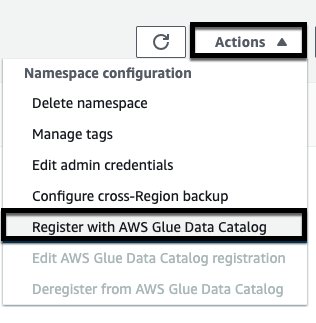
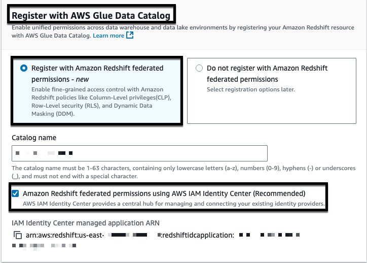
To register the edw-ns namespace with federated permissions:

  1. Open the Amazon Redshift Serverless Namespace console.
  2. Choose your Amazon Redshift Serverless namespace.
  3. Choose Actions, and then select Register with AWS Glue Data Catalog.
  4. Choose Register with Amazon Redshift federated permissions.
  5. Choose Amazon Redshift federated permissions using AWS IAM Identity Center.
  6. Choose Register.
Figure 5: Amazon Redshift data warehouse registration with Glue Data Catalog

Figure 5: Amazon Redshift data warehouse registration with Glue Data Catalog

Figure 6: Amazon Redshift data warehouse registration with Glue Data Catalog

Figure 6: Amazon Redshift data warehouse registration with Glue Data Catalog

Note: IAM Identity Center managed application ARN Data sharing producer IDC connection created would be used.

Configure Amazon Redshift data sharing consumer IDC connection for existing serverless namespace

For cpd-sales-wg and cpd-marketing-wg serverless workgroups, gather the following information from your registered IAM Identity Center connection:

  • IAM Identity Center display name
  • Identity provider namespace
  • IAM Identity Center managed application ARN
  • IAM role for IAM Identity Center access

Run the following SQL command as a database administrator to enable the integration:

CREATE IDENTITY PROVIDER "<IAM Identity Center display name>" TYPE AWSIDC
NAMESPACE '<Identity provider namespace>'
APPLICATION_ARN '<IAM Identity Center managed application ARN>'
IAM_ROLE '<IAM role for IAM Identity Center access>';

To modify an existing identity provider, use the ALTER IDENTITY PROVIDER command:

ALTER IDENTITY PROVIDER "<IAM Identity Center display name>"
NAMESPACE '<Identity provider namespace>';
ALTER IDENTITY PROVIDER "<IAM Identity Center display name>"
IAM_ROLE default | '<IAM role for IAM Identity Center access>';

Data preparation and access setup from producer

In this section, you create the customer and product tables, load sample data, create DDM and RLS policies, attach the policies to database roles and grant SELECT permissions to the roles.

Prepare data on EDW

Connect to the EDW data warehouse as an IDC Admin user and run the following SQL commands.

Create the product table:

CREATE TABLE product (
  product_id VARCHAR(16) NOT NULL,
  product_desc VARCHAR(200),
  current_price NUMERIC(7,2),
  wholesale_cost NUMERIC(7,2),
  category_desc VARCHAR(50),
  launch_status VARCHAR(50)
);

Insert sample product data:

INSERT INTO product 
VALUES 
  ('AAAAAAAAAFNPEAAA','At least concerned authors adopt just brown, federal',7.12,4.12,'Jewelry','launched'),
  ('AAAAAAAAOAAGDAAA','Complex services may not find totally changing accountants. Tiny, available ministers could not know always systems. Hot, male speakers discer',8.08,5.49,'Shoes','planned'),
  ('AAAAAAAAMJJMCAAA','Rows could prevent political, old duties. Just international stairs would regret police. Conditions discard always interesting, warm years. Present jobs shall take nearby relatively dreadful',8.18,5.31,'Jewelry','launched'),
  ('AAAAAAAAKLBLBAAA','Suddenly external sentences believe then by the assets. Simultaneously young feet could not probe separately shortly new men. Forms work again individuals. Images',17.96,7.9,'Shoes','launched'),
  ('AAAAAAAAMBKMCAAA','Clubs see finally materials. Significant objectives sell fairly left, civil power',3.18,3.84,'Books','launched'),
  ('AAAAAAAACPCAAAAA','Perhaps past preferences tell rather to a accounts. Very common feet can command never available final years; minutes expect recent, due employers. Altogether english shoes',9.84,0.19,'Electronics','planned'),
  ('AAAAAAAAFOIABAAA','More responsible characters go left factors. Championships shall stand twice new, important shows. Books could receive too able, national pounds. Central',3.55,2.2,'Books','launched'),
  ('AAAAAAAAKGBIAAAA','High, political changes shall not',9.55,5.25,'Electronics','launched');

Create the customer table:

CREATE TABLE customer (
  customer_id VARCHAR(16),
  first_name VARCHAR(20),
  last_name VARCHAR(30),
  date_of_birth VARCHAR(32),
  birth_country VARCHAR(20),
  email_address VARCHAR(50)
);

Insert sample customer data:

INSERT INTO customer
VALUES
  ('AAAAAAAALAMKHGBA','Regina','Coleman','1926-12-17','GAMBIA','[email protected]'),
  ('AAAAAAAAMCMKHGBA','John','Bell','1980-01-07','PAPUA NEW GUINEA','[email protected]'),
  ('AAAAAAAANNMKHGBA','Jacqueline','Pierre','1951-12-18','SAMOA','[email protected]'),
  ('AAAAAAAANFNKHGBA','Frank','Mackay','1992-03-19','HONG KONG','[email protected]'),
  ('AAAAAAAAOGNKHGBA','Anthony','Miller','1948-02-26','ALGERIA','[email protected]'),
  ('AAAAAAAACPOKHGBA','Bradley','Sawyer','1956-12-25','ZAMBIA','[email protected]'),
  ('AAAAAAAAOIPKHGBA','Robert','Carter','1951-01-01','UNITED STATES','[email protected]'),
  ('AAAAAAAALJPKHGBA','Ola','High','1980-11-19','SUDAN','[email protected]');

Create DDM and RLS policies

Create the masking policy for customer date of birth:

CREATE MASKING POLICY mask_cust_dob  
WITH (date_of_birth VARCHAR(32))  
USING (sha2(date_of_birth, 256)::TEXT);

Create RLS policies for product launch status:

CREATE RLS POLICY product_launch_status  
WITH (launch_status VARCHAR(50))   
USING (launch_status = 'launched');
  
CREATE RLS POLICY product_launch_status_all
WITH (launch_status VARCHAR(50))   
USING (launch_status IN ('launched','planned'));

Create Amazon Redshift DB roles for Sales and Marketing groups

Create the database roles:

CREATE ROLE "AWSIDC:awssso-sales";
CREATE ROLE "AWSIDC:awssso-marketing";

Attach masking policies

Attach the masking policy to both roles:

ATTACH MASKING POLICY mask_cust_dob  
ON dev.public.customer (date_of_birth)  
TO ROLE "AWSIDC:awssso-marketing";
ATTACH MASKING POLICY mask_cust_dob  
ON dev.public.customer (date_of_birth)  
TO ROLE "AWSIDC:awssso-sales";

Attach RLS policies and enable RLS on product table

Attach the RLS policies and enable row-level security:

ATTACH RLS POLICY product_launch_status  
ON dev.public.product  
TO ROLE "AWSIDC:awssso-sales"; 
ATTACH RLS POLICY product_launch_status_all  
ON dev.public.product  
TO ROLE "AWSIDC:awssso-marketing";
ALTER TABLE dev.public.product ROW LEVEL SECURITY ON;

Grant access to tables to roles

Grant SELECT permissions to both roles:

GRANT SELECT ON dev.public.customer TO ROLE "AWSIDC:awssso-sales";
GRANT SELECT ON dev.public.customer TO ROLE "AWSIDC:awssso-marketing";
GRANT SELECT ON dev.public.product TO ROLE "AWSIDC:awssso-sales"; 
GRANT SELECT ON dev.public.product TO ROLE "AWSIDC:awssso-marketing";

Connect to SALES data warehouse using IAM Identity Center

To connect as a Sales Analyst:

  1. Connect to cpd-sales-wg using the IAM Identity Center connection type as user sales-analyst, and then choose Continue.
  2. Choose sales-analyst, and then choose Next.
  3. Enter your password, and then choose Sign in.
  4. Enter your MFA code, and then choose Sign in.

You are now connected to Amazon Redshift Query Editor V2 with a successful connection to cpd-sales-wg as sales-analyst.

Figure 7: Connect to Sales data warehouse as IDC user

Figure 7: Connect to Sales data warehouse as IDC user

Query shared data as Sales Analyst

Query the customer table with dynamic data masking applied:

SELECT * FROM "dev@edw-ns"."public"."customer";

You can successfully access the customer table, but the sensitive information in the date_of_birth column is encrypted.

Figure 8: Result set of customer table

Figure 8: Result set of customer table

Query the product table with row-level security enabled:

SELECT * FROM "dev@edw-ns"."public"."product";

You can successfully access the product table, but only view data for products with a launch_status value of launched.

Figure 9: Result set of product table

Figure 9: Result set of product table

Note: To connect to the data sharing producer onboarded to Amazon Redshift federated permissions as an IDC user, a superuser is required to provide a CONNECT privilege to the IDC user trying to connect. For more information about how to grant the CONNECT privileges to the user, see Connect privileges in the Amazon Redshift Database Developer Guide.

Connect to Marketing data warehouse using IAM Identity Center

To connect as a Marketing Analyst:

  1. Connect to cpd-marketing-wg using the IAM Identity Center connection type as user marketing-analyst, and then choose Continue.
  2. Choose marketing-analyst, and then choose Next.
  3. Enter your password, and then choose Sign in.
  4. Enter your MFA code, and then choose Sign in.

You are now connected to Amazon Redshift Query Editor V2 with a successful connection to cpd-marketing-wg as marketing-analyst.

Figure 10: Connect to Marketing data warehouse as IDC user

Figure 10: Connect to Marketing data warehouse as IDC user

Query shared data as Marketing Analyst

Query the customer table with dynamic data masking applied:

SELECT * FROM "dev@edw-ns"."public"."customer";

You can successfully access the customer table, but the sensitive information in the date_of_birth column is encrypted.

Figure 11: Result set of customer table

Figure 11: Result set of customer table

Query the product table with row-level security enabled:

SELECT * FROM "dev@edw-ns"."public"."product";

You can successfully access the product table and view data for products with launch_status values of both launched and planned.

Figure 12: Result set of product table

Figure 12: Result set of product table

Additional resources

For more information about implementing federated permissions in your environment, see the following resources:

AWS Documentation

AWS Blogs

AWS Demo

Key benefits

  • Reduced administrative overhead – Centralized policy management removes manual replication
  • Consistent security enforcement – Policies apply uniformly across the warehouses and access methods
  • Seamless identity integration – Single sign-on with existing identity providers through trusted identity propagation and role-based access control

Conclusion

This post showed you how Amazon Redshift federated permissions with AWS IAM Identity Center integration helps streamline multi-warehouse data governance by centralizing security policy management. You define dynamic data masking and row-level security policies once in a central Enterprise Data Warehouse, and they automatically enforce across the connected data warehouses in the same account and Region.


About the authors

Raghu Kuppala

Raghu Kuppala

Raghu is an Analytics Specialist Solutions Architect experienced working in the databases, data warehousing, and analytics space. Outside of work, he enjoys trying different cuisines and spending time with his family and friends.

Satesh Sonti

Satesh Sonti

Satesh is a Principal Specialist Solutions Architect based out of Atlanta, specializing in building enterprise data platforms, data warehousing, and analytics solutions. He has over 20 years of experience in building data assets and leading complex data platform programs for banking and insurance clients across the globe.

Sandeep Adwankar

Sandeep Adwankar

Sandeep is a Senior Product Manager with Amazon SageMaker Lakehouse. Based in the California Bay Area, he works with customers around the globe to translate business and technical requirements into products that help customers improve how they manage, secure, and access data.

Sumukh Bapat

Sumukh Bapat

Sumukh is a Software Engineer at AWS. He works on improving customer experience for Amazon Redshift by solving complex problems in authentication, connectivity, and security. His work focuses on identity management, secure access, and distributed database systems.

Praveen Kumar Ramakrishnan

Praveen Kumar Ramakrishnan

Praveen is a Senior Software Engineer at AWS. He has nearly 20 years of experience spanning various domains including filesystems, storage virtualization and network security. At AWS, he focuses on enhancing the Redshift data security.

Ashish Ghodke

Ashish Ghodke

Ashish is a Software Engineer at Amazon Web Services, where he works on identity and access management systems for large-scale cloud services like Amazon Redshift. His work focuses on building secure authentication and single sign-on solutions for distributed systems. He is passionate about distributed systems, cloud security, and building reliable infrastructure at scale.

Enhance data ingestion performance in Amazon Redshift with concurrent inserts

Post Syndicated from Raghu Kuppala original https://aws.amazon.com/blogs/big-data/enhance-data-ingestion-performance-in-amazon-redshift-with-concurrent-inserts/

Amazon Redshift is a fully managed petabyte data warehousing service in the cloud. Its massively parallel processing (MPP) architecture processes data by distributing queries across compute nodes. Each node executes identical query code on its data portion, enabling parallel processing.

Amazon Redshift employs columnar storage for database tables, reducing overall disk I/O requirements. This storage method significantly improves analytic query performance by minimizing data read during queries. Data has become many organizations’ most valuable asset, driving demand for real-time or near real-time analytics in data warehouses. This demand necessitates systems that support simultaneous data loading while maintaining query performance. This post showcases the key improvements in Amazon Redshift concurrent data ingestion operations.

Challenges and pain points for write workloads

In a data warehouse environment, managing concurrent access to data is crucial yet challenging. Customers using Amazon Redshift ingest data using various approaches. For example, you might commonly use INSERT and COPY statements to load data to a table, which are also called pure write operations. You might have requirements for low-latency ingestions to maximize data freshness. To achieve this, you can submit queries concurrently to the same table. To enable this, Amazon Redshift implements snapshot isolation by default. Snapshot isolation provides data consistency when multiple transactions are running simultaneously. Snapshot isolation guarantees that each transaction sees a consistent snapshot of the database as it existed at the start of the transaction, preventing read and write conflicts that could compromise data integrity. With snapshot isolation, read queries are able to execute in parallel, so you can take advantage of the full performance that the data warehouse has to offer.
However, pure write operations execute sequentially. Specifically, pure write operations need to acquire an exclusive lock during the entire transaction. They only release the lock when the transaction has committed the data. In these cases, the performance of the pure write operations is constrained by the speed of serial execution of the writes across sessions.

To understand this better, let’s look at how a pure write operation works. Every pure write operation includes pre-ingestion tasks such as scanning, sorting, and aggregation on the same table. After the pre-ingestion tasks are complete, the data is written to the table while maintaining data consistency. Because the pure write operations run serially, even the pre-ingestion steps ran serially due to lack of concurrency. This means that when multiple pure write operations are submitted concurrently, they are processed one after another, with no parallelization even for the pre-ingestion steps. To improve the concurrency of ingestion to the same table and meet low latency requirements for ingestion, customers often use workarounds through the use of staging tables. Specifically, you can submit INSERT ... VALUES(..) statements into staging tables. Then, you perform joins with other tables, such FACT and DIMENSION tables, prior to appending data using ALTER TABLE APPEND into your target tables. This approach isn’t desirable because it requires you to maintain staging tables and potentially have a larger storage footprint due to data block fragmentation from the use of ALTER TABLE APPEND statements.

In summary, the sequential execution of concurrent INSERT and COPY statements, due to their exclusive locking behavior, creates challenges if you want to maximize the performance and efficiency of your data ingestion workflows in Amazon Redshift. To overcome these limitations, you must adopt workaround solutions, introducing additional complexity and overhead. The following section outlines how Amazon Redshift has addressed these pain points with improvements to concurrent inserts.

Concurrent inserts and its benefits

With Amazon Redshift patch 187, Amazon Redshift has introduced significant improvement in concurrency for data ingestion with support for concurrent inserts. This improves concurrent execution of pure write operations such as COPY and INSERT statements, accelerating the time for you to load data into Amazon Redshift. Specifically, multiple pure write operations are able to progress simultaneously and complete pre-ingestion tasks such as scanning, sorting, and aggregation in parallel.

To visualize this improvement, let’s consider an example of two queries, executed concurrently from different transactions.

The following is query 1 in transaction 1:

INSERT INTO table_a SELECT * FROM table_b WHERE table_b.column_x = 'value_a';

The following is query 2 in transaction 2:

INSERT INTO table_a SELECT * FROM table_c WHERE table_c.column_y = 'value_b'

The following figure illustrates a simplified visualization of pure write operations without concurrent inserts.

Without concurrent inserts, the key components are as follows:

  • First, both pure write operations (INSERT) need to read data from table b and table c, respectively.
  • The segment in pink is the scan step (reading data) and the segment in green is write step (actually inserting the data).
  • In the “Before concurrent inserts” state, both queries would run sequentially. Specifically, the scan step in query 2 waits for the insert step in query 1 to complete before it begins.

For example, consider two identically sized queries across different transactions. Both queries need to scan the same amount of data and insert the same amount of data into the target table. Let’s say both are issued at 10:00 AM. First, query 1 would spend from 10:00 AM to 10:50 AM scanning the data and 10:50 AM to 11:00 AM inserting the data. Next, because query 2 is identical in scan and insertion volumes, query 2 would spend from 11:00 AM to 11:50 AM scanning the data and 11:50 AM to 12:00 PM inserting the data. Both transactions started at 10:00 AM. The end-to-end runtime is 2 hours (transaction 2 ends at 12:00 PM).The following figure illustrates a simplified visualization of pure write operations with concurrent inserts, compared with the previous example.

With concurrent inserts enabled, the scan step of query 1 and query 2 can progress simultaneously. When either of the queries need to insert data, they now do so serially. Let’s consider the same example, with two identically sized queries across different transactions. Both queries need to scan the same amount of data and insert the same amount of data into the target table. Again, let’s say both are issued at 10:00 AM. At 10:00 AM, query 1 and query 2 begin executing concurrently. From 10:00 AM to 10:50 AM, query 1 and query 2 are able to scan the data in parallel. From 10:50 AM to 11:00 AM, query 1 inserts the data into the target table. Next, from 11:00 AM to 11:10 AM, query 2 inserts the data into the target table. The total end-to-end runtime for both transactions is now reduced to 1 hour and 10 minutes, with query 2 completing at 11:10 AM. In this scenario, the pre-ingestion steps (scanning the data) for both queries are able to run concurrently, taking the same amount of time as in the previous example (50 minutes). However, the actual insertion of data into the target table is now executed serially, with query 1 completing the insertion first, followed by query 2. This demonstrates the performance benefits of the concurrent inserts feature in Amazon Redshift. By allowing the pre-ingestion steps to run concurrently, the overall runtime is improved by 50 minutes compared to the sequential execution before the feature was introduced.

With concurrent inserts, pre-ingestion steps are able to progress simultaneously. Pre-ingestion tasks could be one or a combination of tasks, such as scanning, sorting, and aggregation. There are significant performance benefits achieved in the end-to-end runtime of the queries.

Benefits

You can now benefit from these performance improvements without any additional configuration because the concurrent processing is handled automatically by the service. There are multiple benefits from the improvements in concurrent inserts. You can experience the improvement of end-to-end performance of ingestion workloads when you’re writing to the same table. Internal benchmarking shows that concurrent inserts can improve end-to-end runtime by up to 40% for concurrent insert transactions to the same tables. This feature is particularly beneficial for scan-heavy queries (queries that spend more time reading data than they spend time writing data). The higher the ratio of scan:insert in any query, higher the performance improvement expected.

This feature also improves the throughput and performance for multi-warehouse writes through data sharing. Multi-warehouse writes through data sharing helps you scale your write workloads across dedicated Redshift clusters or serverless workgroups, optimizing resource utilization and achieving more predictable performance for your extract, transform, and load (ETL) pipelines. Specifically, in multi-warehouse writes through data sharing, queries from different warehouses can write data on the same table. Concurrent inserts improve the end-to-end performance of these queries by reducing resource contention and enabling them to make progress simultaneously.


The following figure shows the performance improvements from internal tests from concurrent inserts, with the orange bar indicating the performance improvement for multi-warehouse writes through data sharing and the blue bar denoting the performance improvement for concurrent inserts on the same warehouse. As the graph indicates, queries with higher scan components relative to insert components benefit up to 40% with this new feature.

You can also experience additional benefits as a result of using concurrent inserts to manage your ingestion pipelines. When you directly write data to the same tables by using the benefit of concurrent inserts instead of using workarounds with ALTER TABLE APPEND statements, you can reduce your storage footprint. This comes in two forms: first from the elimination of temporary tables, and second from the reduction in table fragmentation from frequent ALTER TABLE APPEND statements. Additionally, you can avoid operational overhead of managing complex workarounds and rely on frequent background and customer-issued VACUUM DELETE operations to manage the fragmentation caused by appending temporary tables to your target tables.

Considerations

Although the concurrent insert enhancements in Amazon Redshift provide significant benefits, it’s important to be aware of potential deadlock scenarios that can arise in a snapshot isolation environment. Specifically, in a snapshot isolation environment, deadlocks can occur in certain conditions when running concurrent write transactions on the same table. The snapshot isolation deadlock happens when concurrent INSERT and COPY statements are sharing a lock and making progress, and another statement needs to perform an operation (UPDATE, DELETE, MERGE, or DDL operation) that requires an exclusive lock on the same table.

Consider the following scenario:

  • Transaction 1:
    INSERT/COPY INTO table_A;

  • Transaction 2:
    INSERT/COPY INTO table_A;
    <UPDATE/DELETE/MERGE/DDL statement> table_A

A deadlock can occur when multiple transactions with INSERT and COPY operations are running concurrently on the same table with a shared lock, and one of those transactions follows its pure write operation with an operation that requires an exclusive lock, such as an UPDATE, MERGE, DELETE, or DDL statement. To avoid the deadlock in these situations, you can separate statements requiring an exclusive lock (UPDATE, MERGE, DELETE, DDL statements) to a different transaction so that INSERT and COPY statements can progress simultaneously, and the statements requiring exclusive locks can execute after them. Alternatively, for transactions with INSERT and COPY statements and MERGE, UPDATE, and DELETE statements on same table, you can include retry logic in your applications to work around potential deadlocks. Refer to Potential deadlock situation for concurrent write transactions involving a single table for more information about deadlocks, and see Concurrent write examples for examples of concurrent transactions.

Conclusion

In this post, we demonstrated how Amazon Redshift has addressed a key challenge: improving concurrent data ingestion performance into a single table. This enhancement can help you meet your requirements for low latency and stricter SLAs when accessing the latest data. The update exemplifies our commitment to implementing critical features in Amazon Redshift based on customer feedback.


About the authors

Raghu Kuppala is an Analytics Specialist Solutions Architect experienced working in the databases, data warehousing, and analytics space. Outside of work, he enjoys trying different cuisines and spending time with his family and friends.

Sumant Nemmani is a Senior Technical Product Manager at AWS. He is focused on helping customers of Amazon Redshift benefit from features that use machine learning and intelligent mechanisms to enable the service to self-tune and optimize itself, ensuring Redshift remains price-performant as they scale their usage.

Gagan Goel is a Software Development Manager at AWS. He ensures that Amazon Redshift features meet customer needs by prioritising and guiding the team in delivering customer-centric solutions, monitor and enhance query performance for customer workloads.

Kshitij Batra is a Software Development Engineer at Amazon, specializing in building resilient, scalable, and high-performing software solutions.

Sanuj Basu is a Principal Engineer at AWS, driving the evolution of Amazon Redshift into a next-generation, exabyte-scale cloud data warehouse. He leads engineering for Redshift’s core data platform — including managed storage, transactions, and data sharing — enabling customers to power seamless multi-cluster analytics and modern data mesh architectures. Sanuj’s work helps Redshift customers break through th

Write queries faster with Amazon Q generative SQL for Amazon Redshift

Post Syndicated from Raghu Kuppala original https://aws.amazon.com/blogs/big-data/write-queries-faster-with-amazon-q-generative-sql-for-amazon-redshift/

Amazon Redshift is a fully managed, AI-powered cloud data warehouse that delivers the best price-performance for your analytics workloads at any scale. Amazon Q generative SQL brings the capabilities of generative AI directly into the Amazon Redshift query editor. Amazon Q generative SQL for Amazon Redshift was launched in preview during AWS re:Invent 2023. With over 85,000 queries executed in preview, Amazon Redshift announced the general availability in September 2024.

Amazon Q generative SQL for Amazon Redshift uses generative AI to analyze user intent, query patterns, and schema metadata to identify common SQL query patterns directly within Amazon Redshift, accelerating the query authoring process for users and reducing the time required to derive actionable data insights. It provides a conversational interface where users can submit queries in natural language within the scope of their current data permissions. Generative SQL uses query history for better accuracy, and you can further improve accuracy through custom context, such as table descriptions, column descriptions, foreign key and primary key definitions, and sample queries. Custom context enhances the AI model’s understanding of your specific data model, business logic, and query patterns, allowing it to generate more relevant and accurate SQL recommendations. It enables you to get insights faster without extensive knowledge of your organization’s complex database schema and metadata.

Within this feature, user data is secure and private. Your data is not shared across accounts. Your queries, data and database schemas are not used to train a generative AI foundational model (FM). Your input is used as contextual prompts to the FM to answer only your queries.

In this post, we show you how to enable the Amazon Q generative SQL feature in the Redshift query editor and use the feature to get tailored SQL commands based on your natural language queries. With Amazon Q, you can spend less time worrying about the nuances of SQL syntax and optimizations, allowing you to concentrate your efforts on extracting invaluable business insights from your data.

Solution overview

At a high level, the feature works as follows:

  1. For generating the SQL code, you can write your query request in plain English within the conversational interface in the Redshift query editor.
  2. The query editor sends the query context to the underlying Amazon Q generative SQL platform, which uses generative AI to generate SQL code recommendations based on your Redshift metadata.
  3. You receive the generated SQL code suggestions within the same chat interface.

The following diagram illustrates this workflow.

Your content processed by generative SQL is not stored or used by AWS for service improvement.

Amazon Q generative SQL uses a large language model (LLM) and Amazon Bedrock to generate the SQL query. AWS uses different techniques, such as prompt engineering and Retrieval Augmented Generation (RAG), to query the model based on your context:

  • The database you’re connected to
  • The schema you’re working on
  • Your query history
  • Optionally, the query history of other users connected to the same endpoint

Amazon Q generative SQL is conversational, and you can ask it to refine a previously generated query.

In the following sections, we demonstrate how to enable the generative SQL feature in the Redshift query editor and use it to generate SQL queries using natural language.

Prerequisites

To get started, you need an Amazon Redshift Serverless endpoint or an Amazon Redshift provisioned cluster. For this post, we use Redshift Serverless. Refer to Easy analytics and cost-optimization with Amazon Redshift Serverless to get started.

Enable the Amazon Q generative SQL feature in the Redshift query editor

If you’re using the feature for the first time, you need to enable the Amazon Q generative SQL feature in the Redshift query editor.

To enable the feature, complete the following steps:

  1. On the Amazon Redshift console, open the Redshift Serverless dashboard.
  2. Choose Query data.

You can also choose Query Editor V2 in the navigation pane of the Amazon Redshift console.

When you open the Redshift query editor, you will see the new icon for Amazon Q next to the database dropdown menu on the top of the query editor console.

If you choose the Amazon Q icon, you will see the message “Amazon Redshift query editor V2 now supports generative SQL functionality. Contact your administrator to activate this feature in Settings.” If you’re not the administrator, you need to work with the account administrator to enable this feature.

  1. If you’re the administrator, choose the hyperlink in the message, or go to the settings icon and choose Generative SQL settings.
  2. In the Generative SQL settings section, select Q generative SQL, which will turn on Amazon Q generative SQL for all users of the account.

Amazon Q generative SQL is personalized to your database and, based on the updates or conversations you have had with the feature, will apply those learnings to other user conversations who connect to the same database with their own credentials. In the generative SQL settings, you can see the instructions to grant the sys:monitor role to a user or role.

  1. Choose Save.

You will receive a confirmation that the Amazon Q generative SQL settings have been successfully updated.

Load notebooks with sample TPC-DS data

The Redshift query editor comes with sample data and SQL notebooks that you can load into a sample database and corresponding schema. For this post, we use TPC-DS for a decision support benchmark.

We start by loading the TPC-DS data into the Redshift database. When you load this data, the schema tpcds is updated with sample data. We also use the provided notebooks with the tpcds schema to run queries to build a query history.

Complete the following steps:

  1. Connect to your Redshift Serverless workgroup or Redshift provisioned cluster.
  2. Navigate to the sample_data_dev database to view the sample databases available for running the generative SQL feature.
  3. Hover over the tpcds schema and choose Open sample notebooks.
  4. In the Create sample database pop-up message, choose Create.

In a few seconds, you will see the notification that the database sample_data_dev is created successfully and tpcds sample data is loaded successfully. Two sample notebooks for the schema are also generated.

  1. Choose Run all on each notebook tab.

This will take a few minutes to run and will establish a query history for the tpcds data.

This step is not mandatory for using the feature for your organization’s data warehouse.

Use Amazon Q to generate SQL queries from natural language

Now that the Amazon Q generative SQL feature is enabled and ready for use, open a new notebook and choose the Amazon Q icon to open a chat pane in the Redshift query editor.

Amazon Q generative SQL is personalized to your schema. It uses metadata from database schemas to improve the SQL query suggestions. Optionally, administrators can allow the use of the account’s query history to further improve the generated SQL. This can be enabled by running the following GRANT commands to provide access to your query history to other roles or users:

GRANT ROLE SYS:MONITOR to "IAMR:role-name";
GRANT ROLE SYS:MONITOR to "IAM:user-name";
GRANT ROLE SYS:MONITOR to "database-username";

This optional step allows users to make query monitoring history available to other users connected to the same database.

Let’s get started with some query examples.

  1. First, make sure you’re connected to sample_data_dev
  2. Let’s ask the query “What are the top 10 stores in sales in 1998?”

This generates a SQL query. Amazon Q generative SQL is also personalized to your data domain. You will notice that it joins to the Store table to retrieve store_name.

  1. Choose Add to notebook under the query to add the generated SQL.

Our query runs successfully and shows that the store able has the most sales.

  1. Amazon Q is personalized to your conversation. Suppose you want to know what the top selling item was for store able. You can ask this question “What was the unique identifier of the top selling item for the store ‘able’?”

The results show the top selling item. However, the query didn’t filter on the year.

  1. Let’s ask Amazon Q to give us the top selling item for store able in 1998. Instead of repeating the whole question again, you can simply ask “Can you filter by the year 1998?”

Now we have the top selling item for store able for 1998.

  1. To display the item description, you can ask the query “Can you modify the query to include its name and description?”

Amazon Q added the join to the item table and the query ran successfully.

Now that we have done some basic queries, let’s do some deeper analysis.

  1. Let’s ask Amazon Q “Can you give me aggregated store sales, for each county by quarter for all years?”

The answer is correct, but let’s ask a follow-up to include the state.

  1. Ask the follow-up question: “Can you include state?”

This answer looks good; you can also add an ORDER BY clause if you want the data sorted or ask Amazon Q to add that.

So far, we have only been looking at store_sales data. The TPC-DS data contains data for other sales channels, including web_sales and catalog_sales.

  1. Let’s ask Amazon Q “Can you give me the total sales for 1998, from different sales channels, using a union of the sales data from different channels?”

Let’s dive deeper into some other capabilities of Amazon Q generative SQL.

  1. Let’s try logging in with a different user and see how Amazon Q generative SQL interacts with that user. We have created User3 and granted the sys:monitor
  2. Logged in as User3, let’s ask the original question of “What are the top 10 stores in sales in 1998?”

Amazon Q generative SQL is able to use the query history and provide SQL recommendations for User3’s prompts because they have access to the system metadata provided through the role sys:monitor.

Safety features

Amazon Q generative SQL has built-in safety features to warn if a generated SQL statement will modify data and will only run based on user permissions. To test this, let’s ask Amazon Q to “delete data from web_sales table.”

Amazon Q gives a message “I detected that this query changes your database. Only run this SQL command if that is appropriate.”

Now, still logged in as User3, choose Run to try to delete the web_sales data.

As expected, User3 gets a permission denied error, because they don’t have the necessary privileges to delete the web_sales table.

Custom context

Custom context is a feature that allows you to provide domain-specific knowledge and preferences, giving you fine-grained control over the SQL generation process.

The custom context is defined in a JSON file, which can be uploaded by the query editor administrator or can be added directly in the Custom context section in Amazon Q generative SQL settings.

This JSON file contains information that helps Amazon Q generative SQL better understand the specific requirements and constraints of your domain, enabling it to generate more targeted and relevant SQL queries.

By providing a custom context, you can influence factors such as:

  • The terminology and vocabulary used in the generated SQL
  • The level of complexity and optimization of the SQL queries
  • The formatting and structure of the SQL statements
  • The data sources and tables that should be considered

The custom context feature empowers you to take a more active role in shaping the SQL generation process, leading to SQL queries that are better suited to your data and business requirements.

In this post, we use the BIRD (BIg Bench for LaRge-scale Database Grounded Text-to-SQL Evaluation) sample dataset, consisting of three tables. BIRD represents a pioneering, cross-domain dataset that examines the impact of extensive database contents on text-to-SQL parsing.

You can load the following BIRD sample dataset into your Redshift data warehouse to experiment with using custom contexts.

For this post, we demonstrate with three custom contexts.

TablesToInclude

TablesToInclude specifies a set of tables that are considered for SQL generation. This field is crucial when you want to limit the scope of SQL queries to a defined subset of available tables. It can help optimize the generation process by reducing unnecessary table references.

Let’s ask Amazon Q “List the distinct translated title and the set code of all cards translated into Spanish.”

This SQL unnecessarily uses the public.cards table. The public.set_translations table contains the data sufficient to answer the question.

We can add the following TablesToInclude custom context JSON:

{
  "resources": [
    {
      "ResourceId":"Serverless:Serverless-workgroup-name",
      "ResourceType": "REDSHIFT_WAREHOUSE",
      "TablesToInclude": [
        "bird.public.set_translations"
      ]
    }
  ]
}

After adding the custom context, the unwanted joins are eliminated and the correct SQL is generated.

ColumnAnnotations

ColumnAnnotations allows you to provide metadata or annotations specific to individual columns in your data tables. These annotations can offer valuable insights into the definitions and characteristics of the columns, which can be beneficial in guiding the SQL generation process.

Let’s ask Amazon Q to “Show me the unconverted mana cost and name for all the cards created by Rob Alexander.”

The generated SQL points to the column convertedmanacost, which doesn’t give a value for unconverted mana cost. The manacost column gives the unconverted mana cost.

Let’s add this using ColumnAnnotations in the custom context JSON:

{
  "resources": [
    {
      "ResourceId": "Serverless: Serverless-workgroup-name",
      "ResourceType": "REDSHIFT_WAREHOUSE",
      "ColumnAnnotations":
         {"bird.public.cards": { "manaCost": "manaCost is the unconverted mana"} }
    }
  ]
}

After the custom context is added, the correct SQL gets generated.

CuratedQueries

CuratedQueries provides a set of predefined question and answer pairs. In this set, the questions are written in natural language and the corresponding answers are the SQL queries that should be generated to address those questions.

These examples serve as a valuable reference point for Amazon Q generative SQL, helping it understand the types of queries it is expected to generate. You can guide Amazon Q generative SQL with the desired format, structure, and content of the SQL queries it should produce.

Let’s ask Amazon Q “List down the name of artists for cards in Chinese Simplified.”

Although the join key multiverseid exists, it is not correct.

Let’s add the following using CuratedQueries in the custom context JSON:

{
  "resources": [
    {
      "ResourceId": "Serverless: Serverless-workgroup-name",
      "ResourceType": "REDSHIFT_WAREHOUSE",
      "CuratedQueries": [
        {
          "Question": "List down the name of artists for cards in Spanish.",
          "Answer": "SELECT artist FROM public.cards c JOIN public.foreign_data f ON c.uuid = f.uuid WHERE f.language = 'Spanish';"
        }
      ]
    }
  ]
}

After the custom context is added, the correct SQL gets generated.

Additional features

In this section, we discuss the supporting features available with Amazon Q generative SQL feature for Redshift query editor:

Provide feedback

Amazon Q generative SQL allows you to provide feedback on the SQL queries it generates, helping improve the quality and relevance of the SQL over time. This feedback mechanism is accessible through the Amazon Q generative SQL interface, where you can indicate whether the generated SQL was helpful or not.

If you find the generated SQL to not be helpful, you can categorize the feedback into the following areas:

  • Incorrect Tables/Columns – This indicates that the SQL references the wrong tables or columns, or is missing essential tables or columns
  • Incorrect Predicates/Literals/Group By – This category covers issues with the SQL’s filter conditions, literal values, or grouping logic
  • Incorrect SQL Structure – This feedback suggests that the overall structure or syntax of the generated SQL is not correct
  • Other – This option allows you to provide feedback that doesn’t fit into the preceding categories

In addition to selecting the appropriate feedback category, you can also provide free text comments to elaborate on the specific issues or inaccuracies you found in the generated SQL. This additional information can be valuable for Amazon Q to better understand the problems and make improvements.

By actively providing this feedback, you play a crucial role in refining the generation capabilities of Amazon Q generative SQL. The feedback you provide helps the service learn from its mistakes, leading to more accurate and relevant SQL queries that better meet your needs over time.

This feedback loop is an important part of Amazon Q generative SQL’s continuous improvement, because it allows the service to adapt and evolve based on your specific requirements and use cases.

Regenerate SQL

The Regenerate SQL option will prompt Amazon Q to generate a new SQL query based on the same natural language prompt, using its learning and improvement capabilities to provide a potentially better-suited response.

Refresh database

By choosing Refresh database, you can instruct Amazon Q generative SQL to re-fetch and update the metadata information about the connected database.

This metadata includes:

  • Schema definitions – The structure and organization of your database schemas
  • Table definitions – The names, columns, and other properties of the tables in your database
  • Column definitions – The data types, names, and other characteristics of the columns within your database tables

Tips and techniques

To get more accurate SQL recommendations from Amazon Q generative SQL, keep in mind the following best practices:

  • Be as specific as possible. Instead of asking for total store sales, ask for total sales across all sales channels if that is what you need.
  • Add your schema to the path. For example:
    set search_path to tpcds;

  • Iterate when you have complex requests and verify the results. For example, ask which county has the most sales in 2000 and follow up with which item had the most sales.
  • Ask follow-up questions to make queries more specific.
  • If an incomplete response is generated, instead of rephrasing the entire request, provide specific instructions to Amazon Q as a continuation to the prior question.

Clean up

To avoid incurring future charges, delete the Redshift cluster you provisioned as part of this post.

Conclusion

Amazon Q generative SQL for Amazon Redshift simplifies query authoring and increases productivity by allowing you to express queries in natural language and receive SQL code recommendations. This post demonstrated how the Amazon Q generative SQL feature can accelerate data analysis by reducing the time required to write SQL queries. By using natural language processing and seamlessly converting it into SQL, you can boost productivity without requiring an in-depth understanding of your organization’s database structures. Importantly, the robust security measures of Amazon Redshift remain fully enforced, and the quality of the generated SQL continues to improve over time by enabling query history sharing across users.

Get started on your Amazon Q generative SQL journey with Amazon Redshift today by implementing the solution in this post or by referring to Interacting with Amazon Q generative SQL. For pricing information, refer to Amazon Q generative SQL pricing. Also, please try other Redshift generative AI features such as Amazon Redshift Integration with Amazon Bedrock and Amazon Redshift Serverless AI-driven scaling and optimization.


About the authors

Raghu Kuppala is an Analytics Specialist Solutions Architect experienced working in the databases, data warehousing, and analytics space. Outside of work, he enjoys trying different cuisines and spending time with his family and friends.

Sushmita Barthakur is a Senior Data Solutions Architect at Amazon Web Services (AWS), supporting Enterprise customers architect their data workloads on AWS. With a strong background in data analytics, she has extensive experience helping customers architect and build enterprise data lakes, ETL workloads, data warehouses and data analytics solutions, both on-premises and the cloud. Sushmita is based out of Tampa, FL and enjoys traveling, reading and playing tennis.

Xiao Qin is a senior applied scientist with the Learned Systems Group (LSG) at Amazon Web Services (AWS). He studies and applies machine learning techniques to solve data management problems. He is one of the developers that build the Amazon Q generative SQL capability.

Erol MurtezaogluErol Murtezaoglu, a Technical Product Manager at AWS, is an inquisitive and enthusiastic thinker with a drive for self-improvement and learning. He has a strong and proven technical background in software development and architecture, balanced with a drive to deliver commercially successful products. Erol highly values the process of understanding customer needs and problems, in order to deliver solutions that exceed expectations.

Phil Bates was a Senior Analytics Specialist Solutions Architect at AWS, before retiring, with over 25 years of data warehouse experience.

Use custom domain names with Amazon Redshift

Post Syndicated from Raghu Kuppala original https://aws.amazon.com/blogs/big-data/use-custom-domain-names-with-amazon-redshift/

Amazon Redshift is a fully managed, petabyte-scale data warehouse service in the cloud. With Amazon Redshift, you can analyze all your data to derive holistic insights about your business and your customers.

Amazon Redshift now supports custom URLs or custom domain names for your data warehouse. You might want to use a custom domain name or CNAME (Canonical Name) for the following reasons:

  • A custom domain name is straightforward to recall and use.
  • Routing connections is less disruptive. The connections from the client are pointed to the DNS record and not the server name. This lets you easily route connections to new clusters in failover or disaster recovery scenarios.
  • You can now obfuscate your server names with a friendly custom domain name.
  • It helps you avoid application code or connectivity changes in case the underlying data warehouse is migrated to a different Region or the endpoint is changed.

In this post, we discuss how you can modify your data warehouse to use custom domain names and how to connect to a data warehouse that has been configured with a custom URL.

Pre-requisites

To get started, you need a registered domain name. You can use Amazon Route 53 or a third-party domain registrar to register a domain.

You also need a validated Secure Sockets Layer (SSL) certificate for your custom endpoints. This is to verify ownership of the domain name and secure communication. You can use AWS Certificate Manager (ACM) to provision, manage, and deploy public SSL/TLS certificates. You need to use verify-full mode, which ensures that the connections are encrypted and verifies that the hostname of the server matches the hostname in the certificate.

Lastly, you need to attach the necessary permissions to the AWS Identity and Access Management (IAM) role that’s assigned to the relevant users and groups that will manage your Redshift data warehouse. These vary depending on if you’re using Amazon Redshift provisioned or Amazon Redshift Serverless. The permissions needed for the required actions are listed in the following table.

Action IAM Permission
Redshift Provisioned Redshift Serverless
Create custom domain for datawarehouse

redshift:CreateCustomDomainAssociation

acm:DescribeCertificate

redshiftServerless:CreateCustomDomainAssociation

acm:DescribeCertificate

Renaming cluster that has custom domain name acm:DescribeCertificate Not needed
Changing certificate for association

redshift:ModifyCustomDomainAssociation

acm:DescribeCertificate

redshiftServerless:UpdateCustomDomainAssociation

acm:DescribeCertificate

Deleting custom domain redshift:DeleteCustomDomainAssociation redshiftServerless:DeleteCustomDomainAssociation
Connecting to the data warehouse using custom domain name redshift:DescribeCustomDomainAssociations Not needed

The following screenshot shows an example of creating an IAM policy on the IAM console.

Creating DNS CNAME entry for custom domain name

The custom domain name typically includes the root domain and a subdomain, like mycluster.mycompany.com. You can either register a new root domain or use an existing one. For more information about registering a new domain with Route 53, refer to Registering a new domain.

After you set that up, you can add a DNS record that points your custom CNAME to the Redshift endpoint. You can find the data warehouse endpoint on the Amazon Redshift console on the cluster detail page.

The following screenshot illustrates locating a provisioned endpoint.

The following screenshot illustrates locating a serverless endpoint.

Now that you have created the CNAME entry, you can request a certificate from ACM. Complete the following steps:

  1. Open the ACM console and choose Request a certificate.
  2. For Fully qualified domain name, enter your custom domain name.
  3. Choose Request.
  4. Confirm that the request is validated by the owner of the domain by checking the status of the certificate.

The status should be Issued.

Now that you have created the CNAME record and certificate, you can create the custom domain URL for your Redshift cluster using the Amazon Redshift console.

Creating custom domain for a provisioned instance

To create a custom domain for a provisioned instance, complete the following steps:

  1. On the Amazon Redshift console, navigate to your provisioned instance detail page.
  2. On the Actions menu, choose Create custom domain name.
  3. For Custom domain name, enter the CNAME record for your Redshift provisioned cluster.
  4. For ACM certificate, choose the appropriate certificate.
  5. Choose Create.

You should now have a custom domain name associated to your provisioned data warehouse. The custom domain name and custom domain certificate ARN values should now be populated with your entries.

Note that sslmode=verify-full will only work for the new custom endpoint. You can’t use this mode with the default endpoint; you can connect to the default endpoint by using other SSL modes like sslmode=verify-ca.

Create a custom domain for a serverless instance

To create a custom domain for a serverless instance, complete the following steps:

  1. On the Amazon Redshift console, navigate to your serverless instance detail page.
  2. On the Actions menu, choose Create custom domain name.
  3. For Custom domain name, enter the CNAME record for your Redshift Serverless workgroup.
  4. For ACM certificate, choose the appropriate certificate.
  5. Choose Create.

You should now have a custom domain name associated to your serverless workgroup. The custom domain name and custom domain certificate ARN values should now be populated with your entries.

Note that, as with a provisioned instance, sslmode=verify-full will only work for the new custom endpoint. You can’t use this mode with the default endpoint; you can connect to the default endpoint by using other SSL modes like sslmode=verify-ca.

Connect using custom domain name

You can now connect to your cluster using the custom domain name. The JDBC URL would be similar to jdbc:redshift://prefix.rootdomain.com:5439/dev?sslmode=verify-full, where prefix.rootdomain.com is your custom domain name and dev is the default database. Use your preferred editor to connect to this URL using your user name and password.

Update the certificate association for your provisioned custom domain

To update the certificate association using the Amazon Redshift console, navigate to your provisioned cluster details page and on the Actions menu, choose Edit custom domain name. Update the domain name and ACM certificate, then choose Save changes.

To change the cluster’s ACM certificate associated to the custom domain using the AWS Command Line Interface (AWS CLI), use the following command:

aws redshift modify-custom-domain-association --cluster-identifier <clustername> --custom-domain-certificate-arn <newCertArn> --custom-domain-name <currentDomainNameOfCluster>

Update the certificate for your serverless custom domain

To update the certificate using the Amazon Redshift console, navigate to your serverless workgroup details page and on the Actions menu, choose Edit custom domain name. Update the domain name and ACM certificate, then choose Save changes.

To change the serverless workgroup’s ACM certificate associated to the custom domain using the AWS CLI, use the following command:

aws redshift-serverless update-custom-domain-association --region <aws-region> ----custom-domain-name <currentCustomDomainName> --custom-domain-certificate-arn <NewCustomdomaincertarn> --workgroup-name<workgroupname>

Delete a custom provisioned domain

To delete your custom domain, navigate to the provisioned cluster details page. On the Actions menu, choose Delete custom domain name. Enter delete to confirm, then choose Delete.

 To use the AWS CLI, use the following code:

aws redshift delete-custom-domain-association --cluster-identifier <ClusterName> --region <ClusterRegion>  --custom-domain-name <currentDomainName>

Delete a custom serverless domain

To delete your custom domain, navigate to the serverless workgroup details page. On the Actions menu, choose Delete custom domain name. Enter delete to confirm, then choose Delete.

To use the AWS CLI, use the following code:

aws redshift-serverless delete-custom-domain-association --workgroup-name <workgroupname> --custom-domain-name <CurrentCustomDomainName>

Conclusion

In this post, we discussed the benefits of using custom domain names for your Redshift data warehouse and the steps needed to associate a custom domain name with the Redshift endpoint. For more information, refer to Using a custom domain name for client connections.


About the Authors

Raghu Kuppala is an Analytics Specialist Solutions Architect experienced working in the databases, data warehousing, and analytics space. Outside of work, he enjoys trying different cuisines and spending time with his family and friends.

Sam Selvan is a Principal Analytics Solution Architect with Amazon Web Services.

Yanzhu Ji is a Product Manager in the Amazon Redshift team. She has experience in product vision and strategy in industry-leading data products and platforms. She has outstanding skill in building substantial software products using web development, system design, database, and distributed programming techniques. In her personal life, Yanzhu likes painting, photography, and playing tennis.

Nikhitha Loyapally is a Senior Software Development Engineer for Amazon Redshift.