Post Syndicated from Yanzhu Ji original https://aws.amazon.com/blogs/big-data/use-the-new-sql-commands-merge-and-qualify-to-implement-and-validate-change-data-capture-in-amazon-redshift/

Amazon Redshift is a fully managed, petabyte-scale data warehouse service in the cloud. Tens of thousands of customers use Amazon Redshift to process exabytes of data every day to power their analytics workloads.

Amazon Redshift has added many features to enhance analytical processing like ROLLUP, CUBE and GROUPING SETS, which were demonstrated in the post Simplify Online Analytical Processing (OLAP) queries in Amazon Redshift using new SQL constructs such as ROLLUP, CUBE, and GROUPING SETS. Amazon Redshift has recently added many SQL commands and expressions. In this post, we talk about two new SQL features, the MERGE command and QUALIFY clause, which simplify data ingestion and data filtering.

One familiar task in most downstream applications is change data capture (CDC) and applying it to its target tables. This task requires examining the source data to determine if it is an update or an insert to existing target data. Without the MERGE command, you needed to test the new dataset against the existing dataset using a business key. When that didn’t match, you inserted new rows in the existing dataset; otherwise, you updated existing dataset rows with new dataset values.

The MERGE command conditionally merges rows from a source table into a target table. Traditionally, this could only be achieved by using multiple insert, update, or delete statements separately. When using multiple statements to update or insert data, there is a risk of inconsistencies between the different operations. Merge operation reduces this risk by ensuring that all operations are performed together in a single transaction.

The QUALIFY clause filters the results of a previously computed window function according to user‑specified search conditions. You can use the clause to apply filtering conditions to the result of a window function without using a subquery. This is similar to the HAVING clause, which applies a condition to further filter rows from a WHERE clause. The difference between QUALIFY and HAVING is that filtered results from the QUALIFY clause could be based on the result of running window functions on the data. You can use both the QUALIFY and HAVING clauses in one query.

In this post, we demonstrate how to use the MERGE command to implement CDC and how to use QUALIFY to simplify validation of those changes.

Solution overview

In this use case, we have a data warehouse, in which we have a customer dimension table that needs to always get the latest data from the source system. This data must also reflect the initial creation time and last update time for auditing and tracking purposes.

A simple way to solve this is to override the customer dimension fully every day; however, that won’t achieve the update tracking, which is an audit mandate, and it might not be feasible to do for bigger tables.

You can load sample data from Amazon S3 by following the instruction here. Using the existing customer table under sample_data_dev.tpcds, we create a customer dimension table and a source table that will contain both updates for existing customers and inserts for new customers. We use the MERGE command to merge the source table data with the target table (customer dimension). We also show how to use the QUALIFY clause to simplify validating the changes in the target table.

To follow along with the steps in this post, we recommend downloading the accompanying notebook, which contains all the scripts to run for this post. To learn about authoring and running notebooks, refer to Authoring and running notebooks.

Prerequisites

You should have the following prerequisites:

• An AWS account
• A Redshift provisioned cluster or Amazon Redshift Serverless endpoint
• tpcds data in the sample_data_dev database (which contains a customer table)

Create and populate the dimension table

We use the existing customer table under sample_data_dev.tpcds to create a customer_dimension table. Complete the following steps:

1. Create a table using a few selected fields, including the business key, and add a couple of maintenance fields for insert and update timestamps:

    -- create the customer dimension table DROP TABLE IF EXISTS customer_dim CASCADE;
   CREATE TABLE customer_dim ( 
   customer_dim_id     bigint GENERATED BY DEFAULT AS IDENTITY(1, 1), 
   c_customer_sk integer NOT NULL ENCODE az64 distkey,
   c_first_name character(20) ENCODE lzo,
   c_last_name character(30) ENCODE lzo,
   c_current_addr_sk integer ENCODE az64,
   c_birth_country character varying(20) ENCODE lzo,
   c_email_address character(50) ENCODE lzo,
   record_insert_ts    timestamp WITHOUT time ZONE DEFAULT current_timestamp ,
   record_upd_ts       timestamp WITHOUT time ZONE DEFAULT NULL
   )
   SORTKEY (c_customer_sk);

2. Populate the dimension table:

   -- populate dimension 
   insert into customer_dim 
          (c_customer_sk, c_first_name,c_last_name, c_current_addr_sk, c_birth_country, c_email_address) 
   select  c_customer_sk, c_first_name,c_last_name, c_current_addr_sk, c_birth_country, c_email_address
   from “sample_data_dev”.”tpcds”.”customer”;

   

3. Validate the row count and the contents of the table:

   -- check customers count and look at sample data
   select count(1) from customer_dim; 
   select * from customer_dim limit 10;

   

Simulate customer table changes

Use the following code to simulate changes made to the table:

-- create a source table with some updates and some inserts
-- Update- Email has changed for 100 customers 
drop table if exists src_customer;
create table src_customer distkey(c_customer_sk) as 
select c_customer_sk , c_first_name , c_last_name, c_current_addr_sk, c_birth_country, ‘x’+c_email_address as c_email_address, getdate() as effective_dt
from   customer_dim 
where  c_email_address is not null
limit 100;


-- also let’s add three completely new customers
insert into src_customer values 
(15000001, ‘Customer#15’,’000001’, 10001 ,’USA’    , ‘Customer#[email protected]’, getdate() ),
(15000002, ‘Customer#15’,’000002’, 10002 ,’MEXICO’ , ‘Customer#[email protected]’, getdate() ),
(15000003, ‘Customer#15’,’000003’, 10003 ,’CANADA’ , ‘Customer#[email protected]’, getdate() );

-- check source count
select count(1) from src_customer;

Merge the source table into the target table

Now you have a source table with some changes you need to merge with the customer dimension table.

Before the MERGE command, this type of task needed two separate UPDATE and INSERT commands to implement:

-- merge changes to dim customer
BEGIN TRANSACTION;
-- update current records
UPDATE customer_dim
SET    c_first_name      = src.c_first_name      ,
       c_last_name       = src.c_last_name       , 
       c_current_addr_sk = src.c_current_addr_sk , 
       c_birth_country   = src.c_birth_country   , 
       c_email_address   = src.c_email_address   ,
       record_upd_ts     = current_timestamp
from   src_customer AS src
where  customer_dim.c_customer_sk = src.c_customer_sk ;
-- Insert new records
INSERT INTO customer_dim (c_customer_sk, c_first_name,c_last_name, c_current_addr_sk, c_birth_country, c_email_address) 
select src.c_customer_sk, src.c_first_name,src.c_last_name, src.c_current_addr_sk, src.c_birth_country, src.c_email_address 
from   src_customer AS src
where  src.c_customer_sk NOT IN (select c_customer_sk from customer_dim);
-- end merge operation
COMMIT TRANSACTION;

The MERGE command uses a more straightforward syntax, in which we use the key comparison result to decide if we perform an update DML operation (when matched) or an insert DML operation (when not matched):

MERGE INTO customer_dim using src_customer AS src ON customer_dim.c_customer_sk = src.c_customer_sk
WHEN MATCHED THEN UPDATE 
SET c_first_name      = src.c_first_name      ,
    c_last_name       = src.c_last_name       , 
    c_current_addr_sk = src.c_current_addr_sk , 
    c_birth_country   = src.c_birth_country   , 
    c_email_address   = src.c_email_address   ,
    record_upd_ts     = current_timestamp
WHEN NOT MATCHED THEN INSERT (c_customer_sk, c_first_name,c_last_name, c_current_addr_sk, c_birth_country, c_email_address) 
                      VALUES (src.c_customer_sk, src.c_first_name,src.c_last_name, src.c_current_addr_sk, src.c_birth_country, src.c_email_address );

Validate the data changes in the target table

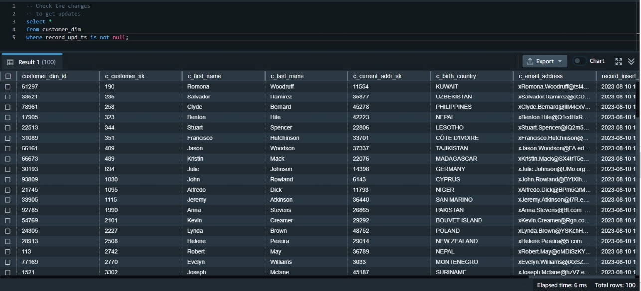
Now we need to validate the data has made it correctly to the target table. We can first check the updated data using the update timestamp. Because this was our first update, we can examine all rows where the update timestamp is not null:

-- Check the changes
-- to get updates
select * 
from customer_dim
where record_upd_ts is not null

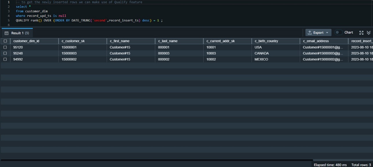
Use QUALIFY to simplify validation of the data changes

We need to examine the data inserted in this table most recently. One way to do that is to rank the data by its insert timestamp and get those with the first rank. This requires using the window function rank() and also requires a subquery to get the results.

Before the availability of QUALIFY, we needed to build that using a subquery like the following:

select customer_dim_id,c_customer_sk ,c_first_name ,c_last_name ,c_current_addr_sk,c_birth_country ,c_email_address ,record_insert_ts ,record_upd_ts 
from 
( select rank() OVER (ORDER BY DATE_TRUNC(‘second’,record_insert_ts) desc) AS rnk, 
         customer_dim_id,c_customer_sk ,c_first_name ,c_last_name ,c_current_addr_sk,c_birth_country ,c_email_address ,record_insert_ts ,record_upd_ts 
  from customer_dim
  where record_upd_ts is null)
where rnk = 1;

The QUALIFY function eliminates the need for the subquery, as in the following code snippet:

-- to get the newly inserted rows we can make use of Qualify feature
select * 
from customer_dim
where record_upd_ts is null
qualify rank() OVER (ORDER BY DATE_TRUNC(‘second’,record_insert_ts) desc) = 1 

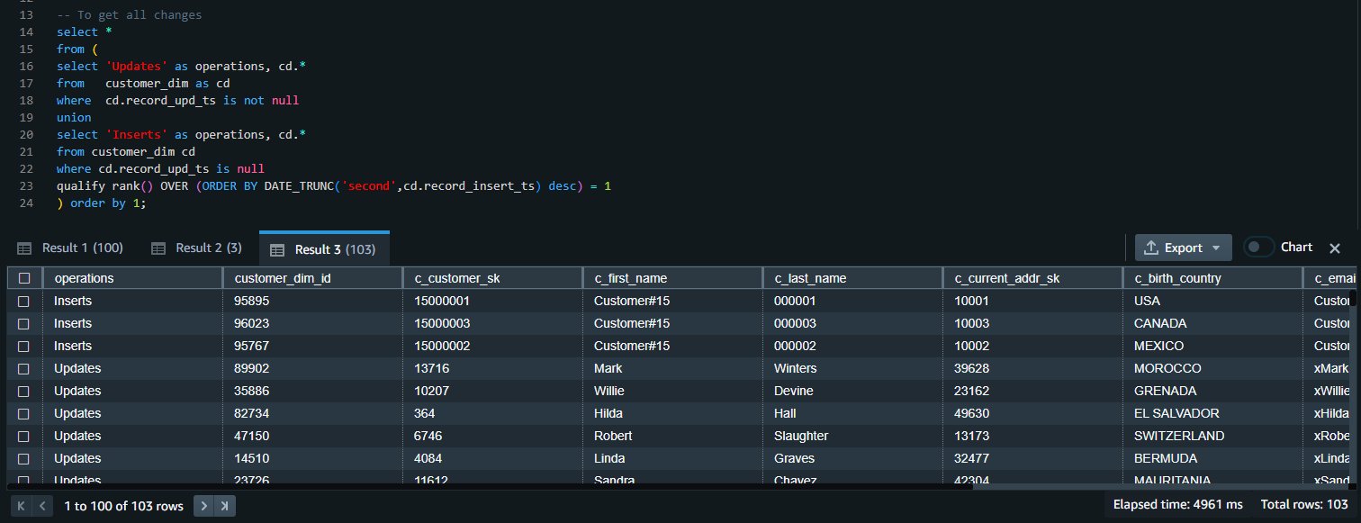
Validate all data changes

We can union the results of both queries to get all the inserts and update changes:

-- To get all changes
select *
from (
select 'Updates' as operations, cd.* 
from   customer_dim as cd
where  cd.record_upd_ts is not null
union 
select 'Inserts' as operations, cd.* 
from customer_dim cd
where cd.record_upd_ts is null
qualify rank() OVER (ORDER BY DATE_TRUNC('second',cd.record_insert_ts) desc) = 1 
) order by 1

Clean up

To clean up the resources used in the post, delete the Redshift provisioned cluster or Redshift Serverless workgroup and namespace you created for this post (this will also drop all the objects created).

If you used an existing Redshift provisioned cluster or Redshift Serverless workgroup and namespace, use the following code to drop these objects:

DROP TABLE IF EXISTS customer_dim CASCADE;
DROP TABLE IF EXISTS src_customer CASCADE;

Conclusion

When using multiple statements to update or insert data, there is a risk of inconsistencies between the different operations. The MERGE operation reduces this risk by ensuring that all operations are performed together in a single transaction. For Amazon Redshift customers who are migrating from other data warehouse systems or who regularly need to ingest fast-changing data into their Redshift warehouse, the MERGE command is a straightforward way to conditionally insert, update, and delete data from target tables based on existing and new source data.

In most analytic queries that use window functions, you may need to use those window functions in your WHERE clause as well. However, this is not permitted, and to do so, you have to build a subquery that contains the required window function and then use the results in the parent query in the WHERE clause. Using the QUALIFY clause eliminates the need for a subquery and therefore simplifies the SQL statement and makes it less difficult to write and read.

We encourage you to start using those new features and give us your feedback. For more details, refer to MERGE and QUALIFY clause.

About the authors

Yanzhu Ji is a Product Manager in the Amazon Redshift team. She has experience in product vision and strategy in industry-leading data products and platforms. She has outstanding skill in building substantial software products using web development, system design, database, and distributed programming techniques. In her personal life, Yanzhu likes painting, photography, and playing tennis.

Ahmed Shehata is a Senior Analytics Specialist Solutions Architect at AWS based on Toronto. He has more than two decades of experience helping customers modernize their data platforms. Ahmed is passionate about helping customers build efficient, performant, and scalable analytic solutions.

Ranjan Burman is an Analytics Specialist Solutions Architect at AWS. He specializes in Amazon Redshift and helps customers build scalable analytical solutions. He has more than 16 years of experience in different database and data warehousing technologies. He is passionate about automating and solving customer problems with cloud solutions.