With EKS Capabilities, you can build and scale Kubernetes applications without managing complex solution infrastructure. Unlike typical in-cluster installations, these capabilities actually run in EKS service-owned accounts that are fully abstracted from customers.
With AWS managing infrastructure scaling, patching, and updates of these cluster capabilities, you can use the enterprise reliability and security without needing to maintain and manage the underlying components.
Here are the capabilities available at launch:
Argo CD – This is a declarative GitOps tool for Kubernetes that provides continuous continuous deployment (CD) capabilities for Kubernetes. It’s broadly adopted, with more than 45% of Kubernetes end-users reporting production or planned production use in the 2024 Cloud Native Computing Foundation (CNCF) Survey.
AWS Controllers for Kubernetes (ACK) – ACK is highly popular with enterprise platform teams in production environments. ACK provides custom resources for Kubernetes that enable the management of AWS Cloud resources directly from within your clusters.
Kube Resource Orchestrator (KRO) – KRO provides a streamlined way to create and manage custom resources in Kubernetes. With KRO, platform teams can create reusable resource bundles that abstract away complexity while remaining natively to the Kubernetes ecosystem.
With these features, you can accelerate and scale your Kubernetes use with fully managed capabilities, using its opinionated but flexible features to build for scale right from the start. It is designed to offer a set of foundational cluster capabilities that layer seamlessly with each other, providing integrated features for continuous deployment, resource orchestration, and composition. You can focus on managing and shipping software without needing to spend time and resources building and managing these foundational platform components.
How it works Platform engineers and cluster administrators can set up EKS Capabilities to offload building and managing custom solutions to provide common foundational services, meaning they can focus on more differentiated features that matter to your business.
Your application developers primarily work with EKS Capabilities as they do other Kubernetes features. They do this by applying declarative configuration to create Kubernetes resources using familiar tools, such as kubectl or through automation from git commit to running code.
Get started with EKS Capabilities To enable EKS Capabilities, you can use the EKS console, AWS Command Line Interface (AWS CLI), eksctl, or other preferred tools. In the EKS console, choose Create capabilities in the Capabilities tab on your existing EKS cluster. EKS Capabilities are AWS resources, and they can be tagged, managed, and deleted.
You can select one or more capabilities to work together. I checked all three capabilities: ArgoCD, ACK, and KRO. However, these capabilities are completely independent and you can pick and choose which capabilities you want enabled on your clusters.
Now you can configure selected capabilities. You should create AWS Identity and Access Management (AWS IAM) roles to enable EKS to operate these capabilities within your cluster. Please note you cannot modify the capability name, namespace, authentication region, or AWS IAM Identity Center instance after creating the capability. Choose Next and review the settings and enable capabilities.
Now you can see and manage created capabilities. Select ArgoCD to update configuration of the capability.
You can see details of ArgoCD capability. Choose Edit to change configuration settings or Monitor ArgoCD to show the health status of the capability for the current EKS cluster.
Choose Go to Argo UI to visualize and monitor deployment status and application health.
Things to know Here are key considerations to know about this feature:
Permissions – EKS Capabilities are cluster-scoped administrator resources, and resource permissions are configured through AWS IAM. For some capabilities, there is additional configuration for single sign-on. For example, Argo CD single sign-on configuration is enabled directly in EKS with a direct integration with IAM Identity Center.
Upgrades – EKS automatically updates cluster capabilities you enable and their related dependencies. It automatically analyzes for breaking changes, patches and updates components as needed, and informs you of conflicts or issues through the EKS cluster insights.
Adoptions – ACK provides resource adoption features that enable migration of existing AWS resources into ACK management. ACK also provides read-only resources which can help facilitate a step-wise migration from provisioned resources with Terraform, AWS CloudFormation into EKS Capabilities.
Now available Amazon EKS Capabilities are now available in commercial AWS Regions. For Regional availability and future roadmap, visit the AWS Capabilities by Region. There are no upfront commitments or minimum fees, and you only pay for the EKS Capabilities and resources that you use. To learn more, visit the EKS pricing page.
The world is in a race to build its first quantum computer capable of solving practical problems not feasible on even the largest conventional supercomputers. While the quantum computing paradigm promises many benefits, it also threatens the security of the Internet by breaking much of the cryptography we have come to rely on.
To mitigate this threat, Cloudflare is helping to migrate the Internet to Post-Quantum (PQ) cryptography. Today, about 50% of traffic to Cloudflare’s edge network is protected against the most urgent threat: an attacker who can intercept and store encrypted traffic today and then decrypt it in the future with the help of a quantum computer. This is referred to as the harvest now, decrypt laterthreat.
However, this is just one of the threats we need to address. A quantum computer can also be used to crack a server’s TLS certificate, allowing an attacker to impersonate the server to unsuspecting clients. The good news is that we already have PQ algorithms we can use for quantum-safe authentication. The bad news is that adoption of these algorithms in TLS will require significant changes to one of the most complex and security-critical systems on the Internet: the Web Public-Key Infrastructure (WebPKI).
The central problem is the sheer size of these new algorithms: signatures for ML-DSA-44, one of the most performant PQ algorithms standardized by NIST, are 2,420 bytes long, compared to just 64 bytes for ECDSA-P256, the most popular non-PQ signature in use today; and its public keys are 1,312 bytes long, compared to just 64 bytes for ECDSA. That’s a roughly 20-fold increase in size. Worse yet, the average TLS handshake includes a number of public keys and signatures, adding up to 10s of kilobytes of overhead per handshake. This is enough to have a noticeable impact on the performance of TLS.
That makes drop-in PQ certificates a tough sell to enable today: they don’t bring any security benefit before Q-day — the day a cryptographically relevant quantum computer arrives — but they do degrade performance. We could sit and wait until Q-day is a year away, but that’s playing with fire. Migrations always take longer than expected, and by waiting we risk the security and privacy of the Internet, which is dear to us.
It’s clear that we must find a way to make post-quantum certificates cheap enough to deploy today by default for everyone — not just those that can afford it. In this post, we’ll introduce you to the plan we’ve brought together with industry partners to the IETF to redesign the WebPKI in order to allow a smooth transition to PQ authentication with no performance impact (and perhaps a performance improvement!). We’ll provide an overview of one concrete proposal, called Merkle Tree Certificates (MTCs), whose goal is to whittle down the number of public keys and signatures in the TLS handshake to the bare minimum required.
But talk is cheap. We knowfromexperience that, as with any change to the Internet, it’s crucial to test early and often. Today we’re announcing our intent to deploy MTCs on an experimental basis in collaboration with Chrome Security. In this post, we’ll describe the scope of this experiment, what we hope to learn from it, and how we’ll make sure it’s done safely.
The WebPKI today — an old system with many patches
Why does the TLS handshake have so many public keys and signatures?
Let’s start with Cryptography 101. When your browser connects to a website, it asks the server to authenticate itself to make sure it’s talking to the real server and not an impersonator. This is usually achieved with a cryptographic primitive known as a digital signature scheme (e.g., ECDSA or ML-DSA). In TLS, the server signs the messages exchanged between the client and server using its secret key, and the client verifies the signature using the server’s public key. In this way, the server confirms to the client that they’ve had the same conversation, since only the server could have produced a valid signature.
If the client already knows the server’s public key, then only 1 signature is required to authenticate the server. In practice, however, this is not really an option. The web today is made up of around a billion TLS servers, so it would be unrealistic to provision every client with the public key of every server. What’s more, the set of public keys will change over time as new servers come online and existing ones rotate their keys, so we would need some way of pushing these changes to clients.
This scaling problem is at the heart of the design of all PKIs.
Trust is transitive
Instead of expecting the client to know the server’s public key in advance, the server might just send its public key during the TLS handshake. But how does the client know that the public key actually belongs to the server? This is the job of a certificate.
A certificate binds a public key to the identity of the server — usually its DNS name, e.g., cloudflareresearch.com. The certificate is signed by a Certification Authority (CA) whose public key is known to the client. In addition to verifying the server’s handshake signature, the client verifies the signature of this certificate. This establishes a chain of trust: by accepting the certificate, the client is trusting that the CA verified that the public key actually belongs to the server with that identity.
Clients are typically configured to trust many CAs and must be provisioned with a public key for each. Things are much easier however, since there are only 100s of CAs instead of billions. In addition, new certificates can be created without having to update clients.
These efficiencies come at a relatively low cost: for those counting at home, that’s +1 signature and +1 public key, for a total of 2 signatures and 1 public key per TLS handshake.
That’s not the end of the story, however. As the WebPKI has evolved, so have these chains of trust grown a bit longer. These days it’s common for a chain to consist of two or more certificates rather than just one. This is because CAs sometimes need to rotatetheir keys, just as servers do. But before they can start using the new key, they must distribute the corresponding public key to clients. This takes time, since it requires billions of clients to update their trust stores. To bridge the gap, the CA will sometimes use the old key to issue a certificate for the new one and append this certificate to the end of the chain.
That’s +1 signature and +1 public key, which brings us to 3 signatures and 2 public keys. And we still have a little ways to go.
Trust but verify
The main job of a CA is to verify that a server has control over the domain for which it’s requesting a certificate. This process has evolved over the years from a high-touch, CA-specific process to a standardized, mostly automated process used for issuing most certificates on the web. (Not all CAs fully support automation, however.) This evolution is marked by a number of security incidents in which a certificate was mis-issued to a party other than the server, allowing that party to impersonate the server to any client that trusts the CA.
Automation helps, but attacks are still possible, and mistakes are almost inevitable. Earlier this year, several certificates for Cloudflare’s encrypted 1.1.1.1 resolver were issued without our involvement or authorization. This apparently occurred by accident, but it nonetheless put users of 1.1.1.1 at risk. (The mis-issued certificates have since been revoked.)
Ensuring mis-issuance is detectable is the job of the Certificate Transparency (CT) ecosystem. The basic idea is that each certificate issued by a CA gets added to a public log. Servers can audit these logs for certificates issued in their name. If ever a certificate is issued that they didn’t request itself, the server operator can prove the issuance happened, and the PKI ecosystem can take action to prevent the certificate from being trusted by clients.
Major browsers, including Firefox and Chrome and its derivatives, require certificates to be logged before they can be trusted. For example, Chrome, Safari, and Firefox will only accept the server’s certificate if it appears in at least two logs the browser is configured to trust. This policy is easy to state, but tricky to implement in practice:
Operating a CT log has historically been fairly expensive. Logs ingest billions of certificates over their lifetimes: when an incident happens, or even just under high load, it can take some time for a log to make a new entry available for auditors.
Clients can’t really audit logs themselves, since this would expose their browsing history (i.e., the servers they wanted to connect to) to the log operators.
The solution to both problems is to include a signature from the CT log along with the certificate. The signature is produced immediately in response to a request to log a certificate, and attests to the log’s intent to include the certificate in the log within 24 hours.
Per browser policy, certificate transparency adds +2 signatures to the TLS handshake, one for each log. This brings us to a total of 5 signatures and 2 public keys in a typical handshake on the public web.
The future WebPKI
The WebPKI is a living, breathing, and highly distributed system. We’ve had to patch it a number of times over the years to keep it going, but on balance it has served our needs quite well — until now.
Previously, whenever we needed to update something in the WebPKI, we would tack on another signature. This strategy has worked because conventional cryptography is so cheap. But 5 signatures and 2 public keys on average for each TLS handshake is simply too much to cope with for the larger PQ signatures that are coming.
The good news is that by moving what we already have around in clever ways, we can drastically reduce the number of signatures we need.
Crash course on Merkle Tree Certificates
Merkle Tree Certificates (MTCs) is a proposal for the next generation of the WebPKI that we are implementing and plan to deploy on an experimental basis. Its key features are as follows:
All the information a client needs to validate a Merkle Tree Certificate can be disseminated out-of-band. If the client is sufficiently up-to-date, then the TLS handshake needs just 1 signature, 1 public key, and 1 Merkle tree inclusion proof. This is quite small, even if we use post-quantum algorithms.
The MTC specification makes certificate transparency a first class feature of the PKI by having each CA run its own log of exactly the certificates they issue.
Let’s poke our head under the hood a little. Below we have an MTC generated by one of our internal tests. This would be transmitted from the server to the client in the TLS handshake:
Looks like your average PEM encoded certificate. Let’s decode it and look at the parameters:
$ openssl x509 -in merkle-tree-cert.pem -noout -text
Certificate:
    Data:
        Version: 3 (0x2)
        Serial Number: 531 (0x213)
        Signature Algorithm: 1.3.6.1.4.1.44363.47.0
        Issuer: 1.3.6.1.4.1.44363.47.1=44363.48.3
        Validity
            Not Before: Oct 21 15:33:26 2025 GMT
            Not After : Oct 28 15:33:26 2025 GMT
        Subject: CN=cloudflareresearch.com
        Subject Public Key Info:
            Public Key Algorithm: id-ecPublicKey
                Public-Key: (256 bit)
                pub:
                    04:70:ed:e1:96:87:b4:22:ef:fb:dc:a9:cd:9c:5c:
                    ef:1e:9e:ab:1b:6d:d7:11:74:7b:76:c8:3c:a1:5f:
                    94:37:45:99:d8:80:e3:5c:24:4f:28:46:b5:bf:84:
                    60:d8:fc:eb:82:5a:c4:4e:33:90:c7:b3:36:51:0c:
                    92:6d:bf:88:27
                ASN1 OID: prime256v1
                NIST CURVE: P-256
        X509v3 extensions:
            X509v3 Key Usage: critical
                Digital Signature
            X509v3 Extended Key Usage:
                TLS Web Server Authentication
            X509v3 Subject Alternative Name:
                DNS:cloudflareresearch.com, DNS:static-ct.cloudflareresearch.com
    Signature Algorithm: 1.3.6.1.4.1.44363.47.0
    Signature Value:
        00:00:00:00:00:00:02:00:00:00:00:00:00:00:02:58:00:e0:
        44:be:03:a5:bd:6a:b7:f2:9e:39:77:4c:16:4c:f8:06:e5:e1:
        55:c0:93:21:c6:79:83:3c:dd:5b:e6:57:89:c0:75:b3:4c:ec:
        75:8a:0b:53:a0:ca:1c:07:0c:1a:92:dd:c7:7c:a2:23:5d:83:
        0e:e4:23:43:38:af:43:20:a8:66:44:34:95:87:ea:2b:f0:0f:
        16:52:bb:ea:67:67:1e:89:36:4f:90:d4:05:55:89:46:f1:b7:
        b6:68:84:d3:57:31:ae:2b:c3:79:31:86:85:9d:24:ed:cf:25:
        a4:5c:fd:8f:f6:76:14:55:dd:67:2e:df:d6:8c:25:0d:52:48:
        c8:e3:fe:f9:7c:e6:a5:30:52:a5:b5:c7:3a:89:a5:c1:f6:4b:
        5b:95:ef:70:b8:91:fc:61:0f:6d:16:de:39:e9:a0:59:49:2b:
        34:71:7c:2a:16:da:c7:af:de:f7:01:94:10:c4:62:d1:f5:00:
        87:bd:e8:a2:f4:df:3b:35:79:27:0e:fc:cc:43:e7:60:5a:df:
        df:06:e8:d3:7e:eb:b3:bf:7b:25:43:0f:34:9a:26:c0:d3:6d:
        5d:0c:28:bc:87:58:58:15:00:00
While some of the parameters probably look familiar, others will look unusual. On the familiar side, the subject and public key are exactly what we might expect: the DNS name is cloudflareresearch.com and the public key is for a familiar signature algorithm, ECDSA-P256. This algorithm is not PQ, of course — in the future we would put ML-DSA-44 there instead.
On the unusual side, OpenSSL appears to not recognize the signature algorithm of the issuer and just prints the raw OID and bytes of the signature. There’s a good reason for this: the MTC does not have a signature in it at all! So what exactly are we looking at?
The trick to leave out signatures is that a Merkle Tree Certification Authority (MTCA) produces its signatureless certificates in batches rather than individually. In place of a signature, the certificate has an inclusion proof of the certificate in a batch of certificates signed by the MTCA.
To understand how inclusion proofs work, let’s think about a slightly simplified version of the MTC specification. To issue a batch, the MTCA arranges the unsigned certificates into a data structure called a Merkle tree that looks like this:
Each leaf of the tree corresponds to a certificate, and each inner node is equal to the hash of its children. To sign the batch, the MTCA uses its secret key to sign the head of the tree. The structure of the tree guarantees that each certificate in the batch was signed by the MTCA: if we tried to tweak the bits of any one of the certificates, the treehead would end up having a different value, which would cause the signature to fail.
An inclusion proof for a certificate consists of the hash of each sibling node along the path from the certificate to the treehead:
Given a validated treehead, this sequence of hashes is sufficient to prove inclusion of the certificate in the tree. This means that, in order to validate an MTC, the client also needs to obtain the signed treehead from the MTCA.
This is the key to MTC’s efficiency:
Signed treeheads can be disseminated to clients out-of-band and validated offline. Each validated treehead can then be used to validate any certificate in the corresponding batch, eliminating the need to obtain a signature for each server certificate.
During the TLS handshake, the client tells the server which treeheads it has. If the server has a signatureless certificate covered by one of those treeheads, then it can use that certificate to authenticate itself. That’s 1 signature,1 public key and 1 inclusion proof per handshake, both for the server being authenticated.
Now, that’s the simplified version. MTC proper has some more bells and whistles. To start, it doesn’t create a separate Merkle tree for each batch, but it grows a single large tree, which is used for better transparency. As this tree grows, periodically (sub)tree heads are selected to be shipped to browsers, which we call landmarks. In the common case browsers will be able to fetch the most recent landmarks, and servers can wait for batch issuance, but we need a fallback: MTC also supports certificates that can be issued immediately and don’t require landmarks to be validated, but these are not as small. A server would provision both types of Merkle tree certificates, so that the common case is fast, and the exceptional case is slow, but at least it’ll work.
Experimental deployment
Ever since early designs for MTCs emerged, we’ve been eager to experiment with the idea. In line with the IETF principle of “running code”, it often takes implementing a protocol to work out kinks in the design. At the same time, we cannot risk the security of users. In this section, we describe our approach to experimenting with aspects of the Merkle Tree Certificates design without changing any trust relationships.
Let’s start with what we hope to learn. We have lots of questions whose answers can help to either validate the approach, or uncover pitfalls that require reshaping the protocol — in fact, an implementation of an early MTC draft by Maximilian Pohl and Mia Celeste did exactly this. We’d like to know:
What breaks? Protocol ossification (the tendency of implementation bugs to make it harder to change a protocol) is an ever-present issue with deploying protocol changes. For TLS in particular, despite having built-in flexibility, time after time we’ve found that if that flexibility is not regularly used, there will be buggy implementations and middleboxes that break when they see things they don’t recognize. TLS 1.3 deployment took years longer than we hoped for this very reason. And more recently, the rollout of PQ key exchange in TLS caused the Client Hello to be split over multiple TCP packets, something that many middleboxes weren’t ready for.
What is the performance impact? In fact, we expect MTCs to reduce the size of the handshake, even compared to today’s non-PQ certificates. They will also reduce CPU cost: ML-DSA signature verification is about as fast as ECDSA, and there will be far fewer signatures to verify. We therefore expect to see a reduction in latency. We would like to see if there is a measurable performance improvement.
What fraction of clients will stay up to date? Getting the performance benefit of MTCs requires the clients and servers to be roughly in sync with one another. We expect MTCs to have fairly short lifetimes, a week or so. This means that if the client’s latest landmark is older than a week, the server would have to fallback to a larger certificate. Knowing how often this fallback happens will help us tune the parameters of the protocol to make fallbacks less likely.
In order to answer these questions, we are implementing MTC support in our TLS stack and in our certificate issuance infrastructure. For their part, Chrome is implementing MTC support in their own TLS stack and will stand up infrastructure to disseminate landmarks to their users.
As we’ve done in past experiments, we plan to enable MTCs for a subset of our free customers with enough traffic that we will be able to get useful measurements. Chrome will control the experimental rollout: they can ramp up slowly, measuring as they go and rolling back if and when bugs are found.
Which leaves us with one last question: who will run the Merkle Tree CA?
Bootstrapping trust from the existing WebPKI
Standing up a proper CA is no small task: it takes years to be trusted by major browsers. That’s why Cloudflare isn’t going to become a “real” CA for this experiment, and Chrome isn’t going to trust us directly.
Instead, to make progress on a reasonable timeframe, without sacrificing due diligence, we plan to “mock” the role of the MTCA. We will run an MTCA (on Workers based on our StaticCT logs), but for each MTC we issue, we also publish an existing certificate from a trusted CA that agrees with it. We call this the bootstrap certificate. When Chrome’s infrastructure pulls updates from our MTCA log, they will also pull these bootstrap certificates, and check whether they agree. Only if they do, they’ll proceed to push the corresponding landmarks to Chrome clients. In other words, Cloudflare is effectively just “re-encoding” an existing certificate (with domain validation performed by a trusted CA) as an MTC, and Chrome is using certificate transparency to keep us honest.
Conclusion
With almost 50% of our traffic already protected by post-quantum encryption, we’re halfway to a fully post-quantum secure Internet. The second part of our journey, post-quantum certificates, is the hardest yet though. A simple drop-in upgrade has a noticeable performance impact and no security benefit before Q-day. This means it’s a hard sell to enable today by default. But here we are playing with fire: migrations always take longer than expected. If we want to keep an ubiquitously private and secure Internet, we need a post-quantum solution that’s performant enough to be enabled by default today.
Merkle Tree Certificates (MTCs) solves this problem by reducing the number of signatures and public keys to the bare minimum while maintaining the WebPKI’s essential properties. We plan to roll out MTCs to a fraction of free accounts by early next year. This does not affect any visitors that are not part of the Chrome experiment. For those that are, thanks to the bootstrap certificates, there is no impact on security.
We’re excited to keep the Internet fast and secure, and will report back soon on the results of this experiment: watch this space! MTC is evolving as we speak, if you want to get involved, please join the IETF PLANTS mailing list.
Open source is the core fabric of the web, and the open source tools that power the modern web depend on the stability and support of the community.
To ensure two major open source projects have the resources they need, we are proud to announce our financial sponsorship to two cornerstone frameworks in the modern web ecosystem: Astro and TanStack.
Critically, we think it’s important we don’t do this alone — for the open web to continue to thrive, we must bet on and support technologies and frameworks that are open and accessible to all, and not beholden to any one company.
Which is why we are also excited to announce that for these sponsorships we are joining forces with our peers at Netlify to sponsor TanStack and Webflow to sponsor Astro.
Why Astro and TanStack? Investing in the Future of the Frontend
Our decision to support Astro and TanStack was deliberate. These two projects represent distinct but complementary visions for the future of web development. One is redefining the architecture for high-performance, content-driven websites, while the other provides a full-stack toolkit for building the most ambitious web applications.
Astro: the framework for the high-performance sites
When it comes to endorsing a technology, we believe actions speak louder than words.
That’s why our support for Astro isn’t just financial—it’s foundational. We run our developer documentation site, developers.cloudflare.com, entirely on Astro. This isn’t a small side project — it’s a critical resource visited by hundreds of thousands of developers every day, with dozens of contributors constantly keeping it updated. For a site like this, performance isn’t a feature; it’s a requirement.
We chose Astro because its core principles mirror our own. Its “zero JS by default” architecture delivers the raw performance and stellar SEO that a content-heavy site demands, ensuring our docs are fast and discoverable. Just as importantly, Astro is framework-agnostic, letting teams use components from React, Vue, or Svelte without vendor lock-in.
Astro makes it easy for our global team to keep content up-to-date and, most importantly, keep our docs blazing fast. Our sponsorship is a direct result of the immense value we’ve experienced firsthand.
Cloudflare’s partnership and support affirms our shared mission: to make the web faster, more open, and better for everyone who builds on it. – Fred K. Schott, Astro Co-creator, Project Steward
Webflow gives marketers, designers, and developers the freedom to build without compromise. Astro shares that same spirit by removing barriers, speeding up workflows, and opening new creative possibilities. Together with Cloudflare and Netlify, we’re helping ensure the tools our community relies on stay open, sustainable, and ready for the future. – Allan Leinwand, Webflow CTO
TanStack Start: the full-stack framework for ambitious applications
If Astro provides the ideal foundation for content-heavy sites, TanStack provides the ideal engine for complex web applications. TanStack is not a single framework but a suite of powerful, headless, and type-safe libraries that solve the hardest problems in modern application development.
Libraries like TanStack Query have become the de facto industry standard for managing asynchronous server state, elegantly solving complex challenges like caching, background refetching, and optimistic updates that once required thousands of lines of fragile, bespoke code. Similarly, TanStack Router brings full type-safety to routing, eliminating an entire class of common bugs, while TanStack Table and TanStack Form provide the robust, headless primitives needed to build sophisticated, data-intensive user interfaces.
And today, TanStack announced its official release of the release candidate for TanStack Start 1.0, taking a big stride towards production-readiness.
TanStack Start is a new full-stack framework that composes these powerful libraries into a cohesive, enterprise-grade development experience. With features like full-document Server-Side Rendering (SSR), streaming, and a “deploy anywhere” architecture, TanStack Start is designed for the modern, serverless edge. It provides the power and type-safety needed for ambitious applications and is a perfect match for deployment environments like Cloudflare Workers.
With Cloudflare alongside us, TanStack can keep raising the bar for fast, scalable, and type-safe tools for powering the next generation of web apps while protecting the openness and freedom developers depend on. – Tanner Linsley, TanStack creator
Supporting an open web is not a nice-to-have for us, but a requirement for us to fulfill our mission to build a better web. Collaborating with Cloudflare on making sure these top projects are funded is the easiest decision we can make! –Mat B, CEO
Joining forces builds a stronger open web
It is not lost on us that this coalition includes companies that compete in the market. We believe this is a feature, not a bug. It demonstrates a shared understanding that we are all building on the same open-source foundations. A healthy, innovative, and sustainable open-source ecosystem is the rising tide that lifts all of our boats.
This joint sponsorship model means Astro and TanStack are more resilient. For you, that means you can build on them with confidence, knowing they aren’t dependent on a single company’s shifting priorities.
With that, show us what you build!
The best way to support open source is to use it, build with it, and contribute back to it. See how easy it is to get started with Astro and TanStack and deploy an application to Cloudflare in minutes with the following framework guides:
Allow us to introduce Cap’n Web, an RPC protocol and implementation in pure TypeScript.
Cap’n Web is a spiritual sibling to Cap’n Proto, an RPC protocol I (Kenton) created a decade ago, but designed to play nice in the web stack. That means:
Like Cap’n Proto, it is an object-capability protocol. (“Cap’n” is short for “capabilities and”.) We’ll get into this more below, but it’s incredibly powerful.
Cap’n Web is more expressive than almost every other RPC system, because it implements an object-capability RPC model. That means it:
Supports bidirectional calling. The client can call the server, and the server can also call the client.
Supports passing functions by reference: If you pass a function over RPC, the recipient receives a “stub”. When they call the stub, they actually make an RPC back to you, invoking the function where it was created. This is how bidirectional calling happens: the client passes a callback to the server, and then the server can call it later.
Similarly, supports passing objects by reference: If a class extends the special marker type RpcTarget, then instances of that class are passed by reference, with method calls calling back to the location where the object was created.
Supports promise pipelining. When you start an RPC, you get back a promise. Instead of awaiting it, you can immediately use the promise in dependent RPCs, thus performing a chain of calls in a single network round trip.
Supports capability-based security patterns.
In short, Cap’n Web lets you design RPC interfaces the way you’d design regular JavaScript APIs – while still acknowledging and compensating for network latency.
The best part is, Cap’n Web is absolutely trivial to set up.
A client looks like this:
import { newWebSocketRpcSession } from "capnweb";

// One-line setup.
let api = newWebSocketRpcSession("wss://example.com/api");

// Call a method on the server!
let result = await api.hello("World");

console.log(result);
And here’s a complete Cloudflare Worker implementing an RPC server:
import { RpcTarget, newWorkersRpcResponse } from "capnweb";

// This is the server implementation.
class MyApiServer extends RpcTarget {
  hello(name) {
    return `Hello, ${name}!`
  }
}

// Standard Workers HTTP handler.
export default {
  fetch(request, env, ctx) {
    // Parse URL for routing.
    let url = new URL(request.url);

    // Serve API at `/api`.
    if (url.pathname === "/api") {
      return newWorkersRpcResponse(request, new MyApiServer());
    }

    // You could serve other endpoints here...
    return new Response("Not found", {status: 404});
  }
}
That’s it. That’s the app.
You can add more methods to MyApiServer, and call them from the client.
You can have the client pass a callback function to the server, and then the server can just call it.
You can define a TypeScript interface for your API, and easily apply it to the client and server.
It just works.
Why RPC? (And what is RPC anyway?)
Remote Procedure Calls (RPC) are a way of expressing communications between two programs over a network. Without RPC, you might communicate using a protocol like HTTP. With HTTP, though, you must format and parse your communications as an HTTP request and response, perhaps designed in REST style. RPC systems try to make communications look like a regular function call instead, as if you were calling a library rather than a remote service. The RPC system provides a “stub” object on the client side which stands in for the real server-side object. When a method is called on the stub, the RPC system figures out how to serialize and transmit the parameters to the server, invoke the method on the server, and then transmit the return value back.
The merits of RPC have been subject to a great deal of debate. RPC is often accused of committing many of the fallacies of distributed computing.
But this reputation is outdated. When RPC was first invented some 40 years ago, async programming barely existed. We did not have Promises, much less async and await. Early RPC was synchronous: calls would block the calling thread waiting for a reply. At best, latency made the program slow. At worst, network failures would hang or crash the program. No wonder it was deemed “broken”.
Things are different today. We have Promise and async and await, and we can throw exceptions on network failures. We even understand how RPCs can be pipelined so that a chain of calls takes only one network round trip. Many large distributed systems you likely use every day are built on RPC. It works.
The fact is, RPC fits the programming model we’re used to. Every programmer is trained to think in terms of APIs composed of function calls, not in terms of byte stream protocols nor even REST. Using RPC frees you from the need to constantly translate between mental models, allowing you to move faster.
When should you use Cap’n Web?
Cap’n Web is useful anywhere where you have two JavaScript applications speaking to each other over a network, including client-to-server and microservice-to-microservice scenarios. However, it is particularly well-suited to interactive web applications with real-time collaborative features, as well as modeling interactions over complex security boundaries.
Cap’n Web is still new and experimental, so for now, a willingness to live on the cutting edge may also be required!
Features, features, features…
Here’s some more things you can do with Cap’n Web.
HTTP batch mode
Sometimes a WebSocket connection is a bit too heavyweight. What if you just want to make a quick one-time batch of calls, but don’t need an ongoing connection?
For that, Cap’n Web supports HTTP batch mode:
import { newHttpBatchRpcSession } from "capnweb";

let batch = newHttpBatchRpcSession("https://example.com/api");

let result = await batch.hello("World");

console.log(result);
(The server is exactly the same as before.)
Note that once you’ve awaited an RPC in the batch, the batch is done, and all the remote references received through it become broken. To make more calls, you need to start over with a new batch. However, you can make multiple calls in a single batch:
let batch = newHttpBatchRpcSession("https://example.com/api");

// We can call make multiple calls, as long as we await them all at once.
let promise1 = batch.hello("Alice");
let promise2 = batch.hello("Bob");

let [result1, result2] = await Promise.all([promise1, promise2]);

console.log(result1);
console.log(result2);
And that brings us to another feature…
Chained calls (Promise Pipelining)
Here’s where things get magical.
In both batch mode and WebSocket mode, you can make a call that depends on the result of another call, without waiting for the first call to finish. In batch mode, that means you can, in a single batch, call a method, then use its result in another call. The entire batch still requires only one network round trip.
let namePromise = batch.getMyName();
let result = await batch.hello(namePromise);

console.log(result);
Notice the initial call to getMyName() returned a promise, but we used the promise itself as the input to hello(), without awaiting it first. With Cap’n Web, this just works: The client sends a message to the server saying: “Please insert the result of the first call into the parameters of the second.”
Or perhaps the first call returns an object with methods. You can call the methods immediately, without awaiting the first promise, like:
let batch = newHttpBatchRpcSession("https://example.com/api");

// Authencitate the API key, returning a Session object.
let sessionPromise = batch.authenticate(apiKey);

// Get the user's name.
let name = await sessionPromise.whoami();

console.log(name);
This works because the promise returned by a Cap’n Web call is not a regular promise. Instead, it’s a JavaScript Proxy object. Any methods you call on it are interpreted as speculative method calls on the eventual result. These calls are sent to the server immediately, telling the server: “When you finish the call I sent earlier, call this method on what it returns.”
Did you spot the security?
This last example shows an important security pattern enabled by Cap’n Web’s object-capability model.
When we call the authenticate() method, after it has verified the provided API key, it returns an authenticated session object. The client can then make further RPCs on the session object to perform operations that require authorization as that user. The server code might look like this:
class MyApiServer extends RpcTarget {
  authenticate(apiKey) {
    let username = await checkApiKey(apiKey);
    return new AuthenticatedSession(username);
  }
}

class AuthenticatedSession extends RpcTarget {
  constructor(username) {
    super();
    this.username = username;
  }

  whoami() {
    return this.username;
  }

  // ...other methods requiring auth...
}
Here’s what makes this work: It is impossible for the client to “forge” a session object. The only way to get one is to call authenticate(), and have it return successfully.
In most RPC systems, it is not possible for one RPC to return a stub pointing at a new RPC object in this way. Instead, all functions are top-level, and can be called by anyone. In such a traditional RPC system, it would be necessary to pass the API key again to every function call, and check it again on the server each time. Or, you’d need to do authorization outside of the RPC system entirely.
This is a common pain point for WebSockets in particular. Due to the design of the web APIs for WebSocket, you generally cannot use headers nor cookies to authorize them. Instead, authorization must happen in-band, by sending a message over the WebSocket itself. But this can be annoying for RPC protocols, as it means the authentication message is “special” and changes the state of the connection itself, affecting later calls. This breaks the abstraction.
The authenticate() pattern shown above neatly makes authentication fit naturally into the RPC abstraction. It’s even type-safe: you can’t possibly forget to authenticate before calling a method requiring auth, because you wouldn’t have an object on which to make the call. Speaking of type-safety…
TypeScript
If you use TypeScript, Cap’n Web plays nicely with it. You can declare your RPC API once as a TypeScript interface, implement in on the server, and call it on the client:
// Shared interface declaration:
interface MyApi {
  hello(name: string): Promise<string>;
}

// On the client:
let api: RpcStub<MyApi> = newWebSocketRpcSession("wss://example.com/api");

// On the server:
class MyApiServer extends RpcTarget implements MyApi {
  hello(name) {
    return `Hello, ${name}!`
  }
}
Now you get end-to-end type checking, auto-completed method names, and so on.
Note that, as always with TypeScript, no type checks occur at runtime. The RPC system itself does not prevent a malicious client from calling an RPC with parameters of the wrong type. This is, of course, not a problem unique to Cap’n Web – JSON-based APIs have always had this problem. You may wish to use a runtime type-checking system like Zod to solve this. (Meanwhile, we hope to add type checking based directly on TypeScript types in the future.)
An alternative to GraphQL?
If you’ve used GraphQL before, you might notice some similarities. One benefit of GraphQL was to solve the “waterfall” problem of traditional REST APIs by allowing clients to ask for multiple pieces of data in one query. For example, instead of making three sequential HTTP calls:
GET /user
GET /user/friends
GET /user/friends/photos
…you can write one GraphQL query to fetch it all at once.
That’s a big improvement over REST, but GraphQL comes with its own tradeoffs:
New language and tooling. You have to adopt GraphQL’s schema language, servers, and client libraries. If your team is all-in on JavaScript, that’s a lot of extra machinery.
Limited composability. GraphQL queries are declarative, which makes them great for fetching data, but awkward for chaining operations or mutations. For example, you can’t easily say: “create a user, then immediately use that new user object to make a friend request, all-in-one round trip.”
Different abstraction model. GraphQL doesn’t look or feel like the JavaScript APIs you already know. You’re learning a new mental model rather than extending the one you use every day.
How Cap’n Web goes further
Cap’n Web solves the waterfall problem without introducing a new language or ecosystem. It’s just JavaScript. Because Cap’n Web supports promise pipelining and object references, you can write code that looks like this:
let user = api.createUser({ name: "Alice" });
let friendRequest = await user.sendFriendRequest("Bob");
What happens under the hood? Both calls are pipelined into a single network round trip:
Create the user.
Take the result of that call (a new User object).
Immediately invoke sendFriendRequest() on that object.
All of this is expressed naturally in JavaScript, with no schemas, query languages, or special tooling required. You just call methods and pass objects around, like you would in any other JavaScript code.
In other words, GraphQL gave us a way to flatten REST’s waterfalls. Cap’n Web lets us go even further: it gives you the power to model complex interactions exactly the way you would in a normal program, with no impedance mismatch.
But how do we solve arrays?
With everything we’ve presented so far, there’s a critical missing piece to seriously consider Cap’n Web as an alternative to GraphQL: handling lists. Often, GraphQL is used to say: “Perform this query, and then, for every result, perform this other query.” For example: “List the user’s friends, and then for each one, fetch their profile photo.”
In short, we need an array.map() operation that can be performed without adding a round trip.
Cap’n Proto, historically, has never supported such a thing.
But with Cap’n Web, we’ve solved it. You can do:
let user = api.authenticate(token);

// Get the user's list of friends (an array).
let friendsPromise = user.listFriends();

// Do a .map() to annotate each friend record with their photo.
// This operates on the *promise* for the friends list, so does not
// add a round trip.
// (wait WHAT!?!?)
let friendsWithPhotos = friendsPromise.map(friend => {
  return {friend, photo: api.getUserPhoto(friend.id))};
}

// Await the friends list with attached photos -- one round trip!
let results = await friendsWithPhotos;
Wait… How!?
.map() takes a callback function, which needs to be applied to each element in the array. As we described earlier, normally when you pass a function to an RPC, the function is passed “by reference”, meaning that the remote side receives a stub, where calling that stub makes an RPC back to the client where the function was created.
But that is NOT what is happening here. That would defeat the purpose: we don’t want the server to have to round-trip to the client to process every member of the array. We want the server to just apply the transformation server-side.
To that end, .map() is special. It does not send JavaScript code to the server, but it does send something like “code”, restricted to a domain-specific, non-Turing-complete language. The “code” is a list of instructions that the server should carry out for each member of the array. In this case, the instructions are:
Invoke api.getUserPhoto(friend.id).
Return an object {friend, photo}, where friend is the original array element and photo is the result of step 1.
But the application code just specified a JavaScript method. How on Earth could we convert this into the narrow DSL?
The answer is record-replay: On the client side, we execute the callback once, passing in a special placeholder value. The parameter behaves like an RPC promise. However, the callback is required to be synchronous, so it cannot actually await this promise. The only thing it can do is use promise pipelining to make pipelined calls. These calls are intercepted by the implementation and recorded as instructions, which can then be sent to the server, where they can be replayed as needed.
And because the recording is based on promise pipelining, which is what the RPC protocol itself is designed to represent, it turns out that the “DSL” used to represent “instructions” for the map function is just the RPC protocol itself. 🤯
Implementation details
JSON-based serialization
Cap’n Web’s underlying protocol is based on JSON – but with a preprocessing step to handle special types. Arrays are treated as “escape sequences” that let us encode other values. For example, JSON does not have an encoding for Date objects, but Cap’n Web does. You might see a message that looks like this:
To encode a literal array, we simply double-wrap it in []:
{
  names: [["Alice", "Bob", "Carol"]]
}
In other words, an array with just one element which is itself an array, evaluates to the inner array literally. An array whose first element is a type name, evaluates to an instance of that type, where the remaining elements are parameters to the type.
Note that only a fixed set of types are supported: essentially, “structured clonable” types, and RPC stub types.
On top of this basic encoding, we define an RPC protocol inspired by Cap’n Proto – but greatly simplified.
RPC protocol
Since Cap’n Web is a symmetric protocol, there is no well-defined “client” or “server” at the protocol level. There are just two parties exchanging messages across a connection. Every kind of interaction can happen in either direction.
In order to make it easier to describe these interactions, I will refer to the two parties as “Alice” and “Bob”.
Alice and Bob start the connection by establishing some sort of bidirectional message stream. This may be a WebSocket, but Cap’n Web also allows applications to define their own transports. Each message in the stream is JSON-encoded, as described earlier.
Alice and Bob each maintain some state about the connection. In particular, each maintains an “export table”, describing all the pass-by-reference objects they have exposed to the other side, and an “import table”, describing the references they have received. Alice’s exports correspond to Bob’s imports, and vice versa. Each entry in the export table has a signed integer ID, which is used to reference it. You can think of these IDs like file descriptors in a POSIX system. Unlike file descriptors, though, IDs can be negative, and an ID is never reused over the lifetime of a connection.
At the start of the connection, Alice and Bob each populate their export tables with a single entry, numbered zero, representing their “main” interfaces. Typically, when one side is acting as the “server”, they will export their main public RPC interface as ID zero, whereas the “client” will export an empty interface. However, this is up to the application: either side can export whatever they want.
From there, new exports are added in two ways:
When Alice sends a message to Bob that contains within it an object or function reference, Alice adds the target object to her export table. IDs assigned in this case are always negative, starting from -1 and counting downwards.
Alice can send a “push” message to Bob to request that Bob add a value to his export table. The “push” message contains an expression which Bob evaluates, exporting the result. Usually, the expression describes a method call on one of Bob’s existing exports – this is how an RPC is made. Each “push” is assigned a positive ID on the export table, starting from 1 and counting upwards. Since positive IDs are only assigned as a result of pushes, Alice can predict the ID of each push she makes, and can immediately use that ID in subsequent messages. This is how promise pipelining is achieved.
After sending a push message, Alice can subsequently send a “pull” message, which tells Bob that once he is done evaluating the “push”, he should proactively serialize the result and send it back to Alice, as a “resolve” (or “reject”) message. However, this is optional: Alice may not actually care to receive the return value of an RPC, if Alice only wants to use it in promise pipelining. In fact, the Cap’n Web implementation will only send a “pull” message if the application has actually awaited the returned promise.
Putting it together, a code sequence like this:
{
  names: [["Alice", "Bob", "Carol"]]
}
Might produce a message exchange like this:
// Call api.getByName(). `api` is the server's main export, so has export ID 0.
-> ["push", ["pipeline", 0, "getMyName", []]
// Call api.hello(namePromise). `namePromise` refers to the result of the first push,
// so has ID 1.
-> ["push", ["pipeline", 0, "hello", [["pipeline", 1]]]]
// Ask that the result of the second push be proactively serialized and returned.
-> ["pull", 2]
// Server responds.
<- ["resolve", 2, "Hello, Alice!"]
Cap’n Web is new and still highly experimental. There may be bugs to shake out. But, we’re already using it today. Cap’n Web is the basis of the recently-launched “remote bindings” feature in Wrangler, allowing a local test instance of workerd to speak RPC to services in production. We’ve also begun to experiment with it in various frontend applications – expect more blog posts on this in the future.
In any case, Cap’n Web is open source, and you can start using it in your own projects now.
At Cloudflare, we believe that helping build a better Internet means encouraging a healthy ecosystem of options for how people can connect safely and quickly to the resources they need. Sometimes that means we tackle immense, Internet-scale problems with established partners. And sometimes that means we support and partner with fantastic open teams taking big bets on the next generation of tools.
To that end, today we are excited to announce our support of two independent, open source projects: Ladybird, an ambitious project to build a completely independent browser from the ground up, and Omarchy, an opinionated Arch Linux setup for developers.
Two open source projects strengthening the open Internet
Cloudflare has a long history of supporting open-source software – both through our own projects shared with the community and external projects that we support. We see our sponsorship of Ladybird and Omarchy as a natural extension of these efforts in a moment where energy for a diverse ecosystem is needed more than ever.
Ladybird, a new and independent browser
Most of us spend a significant amount of time using a web browser – in fact, you’re probably using one to read this blog! The beauty of browsers is that they help users experience the open Internet, giving you access to everything from the largest news publications in the world to a tiny website hosted on a Raspberry Pi.
Unlike dedicated apps, browsers reduce the barriers to building an audience for new services and communities on the Internet. If you are launching something new, you can offer it through a browser in a world where most people have absolutely zero desire to install an app just to try something out. Browsers help encourage competition and new ideas on the open web.
While the openness of how browsers work has led to an explosive growth of services on the Internet, browsers themselves have consolidated to a tiny handful of viable options. There’s a high probability you’re reading this on a Chromium-based browser, like Google’s Chrome, along with about 65% of users on the Internet. However, that consolidation has also scared off new entrants in the space. If all browsers ship on the same operating systems, powered by the same underlying technology, we lose out on potential privacy, security and performance innovations that could benefit developers and everyday Internet users.
A screenshot of Cloudflare Workers developer docs in Ladybird
This is where Ladybird comes in: it’s not Chromium based – everything is built from scratch. The Ladybird project has two main components: LibWeb, a brand-new rendering engine, and LibJS, a brand-new JavaScript engine with its own parser, interpreter, and bytecode execution engine.
Building an engine that can correctly and securely render the modern web is a monumental task that requires deep technical expertise and navigating decades of specifications governed by standards bodies like the W3C and WHATWG. And because Ladybird implements these standards directly, it also stress-tests them in practice. Along the way, the project has found, reported, and sometimes fixed countless issues in the specifications themselves, contributions that strengthen the entire web platform for developers, browser vendors, and anyone who may attempt to build a browser in the future.
Whether to build something from scratch or not is a perennial source of debate between software engineers, but absent the pressures of revenue or special interests, we’re excited about the ways Ladybird will prioritize privacy, performance, and security, potentially in novel ways that will influence the entire ecosystem.
A screenshot of the Omarchy development environment
Omarchy, an independent development environment
Developers deserve choice, too. Beyond the browser, a developer’s operating system and environment is where they spend a ton of time – and where a few big players have become the dominant choice. Omarchy challenges this by providing a complete, opinionated Arch Linux distribution that transforms a bare installation into a modern development workstation that developers are excited about.
Perfecting one’s development environment can be a career-long art, but learning how to do so shouldn’t be a barrier to beginning to code. The beauty of Omarchy is that it makes Linux approachable to more developers by doing most of the setup for them, making it look good, and then making it configurable. Omarchy provides most of the tools developers need – like Neovim, Docker, and Git – out of the box, and tons of other features.
At its core, Omarchy embraces Linux for all of its complexity and configurability, and makes a version of it that is accessible and fun to use for developers that don’t have a deep background in operating systems. Projects like this ensure that a powerful, independent Linux desktop remains a compelling choice for people building the next generation of applications and Internet infrastructure.
Our support comes with no strings attached
We want to be very clear here: we are supporting these projects because we believe the Internet can be better if these projects, and more like them, succeed. No requirement to use our technology stack or any arrangement like that. We are happy to partner with great teams like Ladybird and Omarchy simply because we believe that our missions have real overlap.
Notes from the teams
Ladybird is still in its early days, with an alpha release planned for 2026, but we encourage anyone who is interested to consider contributing to the open source codebase as they prepare for launch.
“Cloudflare knows what it means to build critical web infrastructure on the server side. With Ladybird, we’re tackling the near-monoculture on the client side, because we believe it needs multiple implementations to stay healthy, and we’re extremely thankful for their support in that mission.”
– Andreas Kling, Founder, Ladybird
Omarchy 3.0 was released just last week with faster installation and increased Macbook compatibility, so if you’ve been Linux-curious for a while now, we encourage you to try it out!
“Cloudflare’s support of Omarchy has ensured we have the fastest ISO and package delivery from wherever you are in the world. Without a need to manually configure mirrors or deal with torrents. The combo of a super CDN, great R2 storage, and the best DDoS shield in the business has been a huge help for the project.”
– David Heinemeier Hansson, Creator of Omarchy and Ruby on Rails
A better Internet is one where people have more choice in how they browse and develop new software. We’re incredibly excited about the potential of Ladybird, Omarchy, and other audacious projects that support a free and open Internet.
Today we are adding Qwen models from Alibaba in Amazon Bedrock. With this launch, Amazon Bedrock continues to expand model choice by adding access to Qwen3 open weight foundation models (FMs) in a full managed, serverless way. This release includes four models: Qwen3-Coder-480B-A35B-Instruct, Qwen3-Coder-30B-A3B-Instruct, Qwen3-235B-A22B-Instruct-2507, and Qwen3-32B (Dense). Together, these models feature both mixture-of-experts (MoE) and dense architectures, providing flexible options for different application requirements.
Amazon Bedrock provides access to industry-leading FMs through a unified API without requiring infrastructure management. You can access models from multiple model providers, integrate models into your applications, and scale usage based on workload requirements. With Amazon Bedrock, customer data is never used to train the underlying models. With the addition of Qwen3 models, Amazon Bedrock offers even more options for use cases like:
Code generation and repository analysis with extended context understanding
Building agentic workflows that orchestrate multiple tools and APIs for business automation
Balancing AI costs and performance using hybrid thinking modes for adaptive reasoning
Qwen3 models in Amazon Bedrock These four Qwen3 models are now available in Amazon Bedrock, each optimized for different performance and cost requirements:
Qwen3-Coder-480B-A35B-Instruct – This is a mixture-of-experts (MoE) model with 480B total parameters and 35B active parameters. It’s optimized for coding and agentic tasks and achieves strong results in benchmarks such as agentic coding, browser use, and tool use. These capabilities make it suitable for repository-scale code analysis and multistep workflow automation.
Qwen3-Coder-30B-A3B-Instruct – This is a MoE model with 30B total parameters and 3B active parameters. Specifically optimized for coding tasks and instruction-following scenarios, this model demonstrates strong performance in code generation, analysis, and debugging across multiple programming languages.
Qwen3-235B-A22B-Instruct-2507 – This is an instruction-tuned MoE model with 235B total parameters and 22B active parameters. It delivers competitive performance across coding, math, and general reasoning tasks, balancing capability with efficiency.
Qwen3-32B (Dense) – This is a dense model with 32B parameters. It is suitable for real-time or resource-constrained environments such as mobile devices and edge computing deployments where consistent performance is critical.
Architectural and functional features in Qwen3 The Qwen3 models introduce several architectural and functional features:
MoE compared with dense architectures – MoE models such as Qwen3-Coder-480B-A35B, Qwen3-Coder-30B-A3B-Instruct, and Qwen3-235B-A22B-Instruct-2507, activate only part of the parameters for each request, providing high performance with efficient inference. The dense Qwen3-32B activates all parameters, offering more consistent and predictable performance.
Agentic capabilities – Qwen3 models can handle multi-step reasoning and structured planning in one model invocation. They can generate outputs that call external tools or APIs when integrated into an agent framework. The models also maintain extended context across long sessions. In addition, they support tool calling to allow standardized communication with external environments.
Hybrid thinking modes – Qwen3 introduces a hybrid approach to problem-solving, which supports two modes: thinking and non-thinking. The thinking mode applies step-by-step reasoning before delivering the final answer. This is ideal for complex problems that require deeper thought. Whereas the non-thinking mode provides fast and near-instant responses for less complex tasks where speed is more important than depth. This helps developers manage performance and cost trade-offs more effectively.
Long-context handling – The Qwen3-Coder models support extended context windows, with up to 256K tokens natively and up to 1 million tokens with extrapolation methods. This allows the model to process entire repositories, large technical documents, or long conversational histories within a single task.
When to use each model The four Qwen3 models serve distinct use cases. Qwen3-Coder-480B-A35B-Instruct is designed for complex software engineering scenarios. It’s suited for advanced code generation, long-context processing such as repository-level analysis, and integration with external tools. Qwen3-Coder-30B-A3B-Instruct is particularly effective for tasks such as code completion, refactoring, and answering programming-related queries. If you need versatile performance across multiple domains, Qwen3-235B-A22B-Instruct-2507 offers a balance, delivering strong general-purpose reasoning and instruction-following capabilities while leveraging the efficiency advantages of its MoE architecture. Qwen3-32B (Dense) is appropriate for scenarios where consistent performance, low latency, and cost optimization are important.
Getting started with Qwen models in Amazon Bedrock To begin using Qwen models, in the Amazon Bedrock console, I choose Model Access from the Configure and learn section of the navigation pane. I then navigate to the Qwen models to request access. In the Chat/Text Playground section of the navigation pane, I can quickly test the new Qwen models with my prompts.
To integrate Qwen3 models into my applications, I can use any AWS SDKs. The AWS SDKs include access to the Amazon Bedrock InvokeModel and Converse API. I can also use these model with any agentic framework that supports Amazon Bedrock and deploy the agents using Amazon Bedrock AgentCore. For example, here’s the Python code of a simple agent with tool access built using Strands Agents:
from strands import Agent
from strands_tools import calculator

agent = Agent(
    model="qwen.qwen3-coder-480b-instruct-v1:0",
    tools=[calculator]
)

agent("Tell me the square root of 42 ^ 9")

with open("function.py", 'r') as f:
    my_function_code = f.read()

agent(f"Help me optimize this Python function for better performance:\n\n{my_function_code}")
Now available Qwen models are available today in the following AWS Regions:
Qwen3-Coder-480B-A35B-Instruct is available in the US West (Oregon), Asia Pacific (Mumbai, Tokyo), and Europe (London, Stockholm) Regions.
Qwen3-Coder-30B-A3B-Instruct, Qwen3-235B-A22B-Instruct-2507, and Qwen3-32B are available in the US East (N. Virginia), US West (Oregon), Asia Pacific (Mumbai, Tokyo), Europe (Ireland, London, Milan, Stockholm), and South America (São Paulo) Regions.
In March, Amazon Web Services (AWS) became the first cloud service provider to deliver DeepSeek-R1 in a serverless way by launching it as a fully managed, generally available model in Amazon Bedrock. Since then, customers have used DeepSeek-R1’s capabilities through Amazon Bedrock to build generative AI applications, benefiting from the Bedrock’s robust guardrails and comprehensive tooling for safe AI deployment.
Today, I am excited to announce DeepSeek-V3.1 is now available as a fully managed foundation model in Amazon Bedrock. DeepSeek-V3.1 is a hybrid open weight model that switches between thinking mode (chain-of-thought reasoning) for detailed step-by-step analysis and non-thinking mode (direct answers) for faster responses.
According to DeepSeek, the thinking mode of DeepSeek-V3.1 achieves comparable answer quality with better results, stronger multi-step reasoning for complex search tasks, and big gains in thinking efficiency compared with DeepSeek-R1-0528.
DeepSeek-V3.1 model performance in tool usage and agent tasks has significantly improved through post-training optimization compared to previous DeepSeek models. DeepSeek-V3.1 also supports over 100 languages with near-native proficiency, including significantly improved capability in low-resource languages lacking large monolingual or parallel corpora. You can build global applications to deliver enhanced accuracy and reduced hallucinations compared to previous DeepSeek models, while maintaining visibility into its decision-making process.
Here are your key use cases using this model:
Code generation – DeepSeek-V3.1 excels in coding tasks with improvements in software engineering benchmarks and code agent capabilities, making it ideal for automated code generation, debugging, and software engineering workflows. It performs well on coding benchmarks while delivering high-quality results efficiently.
Agentic AI tools – The model features enhanced tool calling through post-training optimization, making it strong in tool usage and agentic workflows. It supports structured tool calling, code agents, and search agents, positioning it as a solid choice for building autonomous AI systems.
Enterprise applications – DeepSeek models are integrated into various chat platforms and productivity tools, enhancing user interactions and supporting customer service workflows. The model’s multilingual capabilities and cultural sensitivity make it suitable for global enterprise applications.
As I mentioned in my previous post, when implementing publicly available models, give careful consideration to data privacy requirements when implementing in your production environments, check for bias in output, and monitor your results in terms of data security, responsible AI, and model evaluation.
Get started with the DeepSeek-V3.1 model in Amazon Bedrock If you’re new to using the DeepSeek-V3.1 model, go to the Amazon Bedrock console, choose Model access under Bedrock configurations in the left navigation pane. To access the fully managed DeepSeek-V3.1 model, request access for DeepSeek-V3.1 in the DeepSeek section. You’ll then be granted access to the model in Amazon Bedrock.
Next, to test the DeepSeek-V3.1 model in Amazon Bedrock, choose Chat/Text under Playgrounds in the left menu pane. Then choose Select model in the upper left, and select DeepSeek as the category and DeepSeek-V3.1 as the model. Then choose Apply.
Using the selected DeepSeek-V3.1 model, I run the following prompt example about technical architecture decision.
Outline the high-level architecture for a scalable URL shortener service like bit.ly. Discuss key components like API design, database choice (SQL vs. NoSQL), how the redirect mechanism works, and how you would generate unique short codes.
You can turn the thinking on and off by toggling Model reasoning mode to generate a response’s chain of thought prior to the final conclusion.
Last week, Strands Agents, AWS open source for agentic AI SDK just hit 1 million downloads and earned 3,000+ GitHub Stars less than 4 months since launching as a preview in May 2025. With Strands Agents, you can build production-ready, multi-agent AI systems in a few lines of code.
We’ve continuously improved features including support for multi-agent patterns, A2A protocol, and Amazon Bedrock AgentCore. You can use a collection of sample implementations to help you get started with building intelligent agents using Strands Agents. We always welcome your contribution and feedback to our project including bug reports, new features, corrections, or additional documentation.
Here is the latest research article of Amazon Science about the future of agentic AI and questions that scientists are asking about agent-to-agent communications, contextual understanding, common sense reasoning, and more. You can understand the technical topic of agentic AI with with relatable examples, including one about our personal behaviors about leaving doors open or closed, locked or unlocked.
Last week’s launches Here are some launches that got my attention:
Amazon EC2 M4 and M4 Pro Mac instances – New M4 Mac instances offer up to 20% better application build performance compared to M2 Mac instances, while M4 Pro Mac instances deliver up to 15% better application build performance compared to M2 Pro Mac instances. These instances are ideal for building and testing applications for Apple platforms such as iOS, macOS, iPadOS, tvOS, watchOS, visionOS, and Safari.
LocalStack integration in Visual Studio Code (VS Code) – You can use LocalStack to locally emulate and test your serverless applications using the familiar VS Code interface without switching between tools or managing complex setup, thus simplifying your local serverless development process.
AWS CloudTrail MCP Server – New AWS CloudTrail MCP server allows AI assistants to analyze API calls, track user activities, and perform advanced security analysis across your AWS environment through natural language interactions. You can explore more AWS MCP servers for working with AWS service resources.
Amazon CloudFront support for IPv6 origins – Your applications can send IPv6 traffic all the way to their origins, allowing them to meet their architectural and regulatory requirements for IPv6 adoption. End-to-end IPv6 support improves network performance for end users connecting over IPv6 networks, and also removes concerns for IPv4 address exhaustion for origin infrastructure.
For a full list of AWS announcements, be sure to keep an eye on the What’s New with AWS? page.
Other AWS news Here are some additional news items that you might find interesting:
A city in the palm of your hand – Check out this interactive feature that explains how our AWS Trainium chip designers think like city planners, optimizing every nanometer to move data at near light speed.
Measuring the effectiveness of software development tools and practices – Read how Amazon developers that identified specific challenges before adopting AI tools cut costs by 15.9% year-over-year using our cost-to-serve-software framework (CTS-SW). They deployed more frequently and reduced manual interventions by 30.4% by focusing on the right problems first.
Become an AWS Cloud Club Captain – Join a growing network of student cloud enthusiasts by becoming an AWS Cloud Club Captain! As a Captain, you’ll get to organize events and building cloud communities while developing leadership skills. Application window is open September 1-28, 2025.
Upcoming AWS events Check your calendars and sign up for these upcoming AWS events as well as AWS re:Invent and AWS Summits:
AWS AI Agent Global Hackathon – This is your chance to dive deep into our powerful generative AI stack and create something truly awesome. From September 8 to October 20, you have the opportunity to create AI agents using AWS suite of AI services, competing for over $45,000 in prizes and exclusive go-to-market opportunities.
AWS Gen AI Lofts – You can learn AWS AI products and services with exclusive sessions and meet industry-leading experts, and have valuable networking opportunities with investors and peers. Register in your nearest city: Mexico City (September 30–October 2), Paris (October 7–21), London (Oct 13–21), and Tel Aviv (November 11–19).
AWS Community Days – Join community-led conferences that feature technical discussions, workshops, and hands-on labs led by expert AWS users and industry leaders from around the world: Aotearoa and Poland (September 18), South Africa (September 20), Bolivia (September 20), Portugal (September 27), Germany (October 7), and Hungary (October 16).
AWS is committed to bringing you the most advanced foundation models (FMs) in the industry, continuously expanding our selection to include groundbreaking models from leading AI innovators so that you always have access to the latest advancements to drive your business forward.
These open weight models excel at coding, scientific analysis, and mathematical reasoning, with performance comparable to leading alternatives. Both models support a 128K context window and provide adjustable reasoning levels (low/medium/high) to match your specific use case requirements. The models support external tools to enhance their capabilities and can be used in an agentic workflow, for example, using a framework like Strands Agents.
With Amazon Bedrock and Amazon SageMaker JumpStart, AWS gives you the freedom to innovate with access to hundreds of FMs from leading AI companies, including OpenAI open weight models. With our comprehensive selection of models, you can match your AI workloads to the perfect model every time.
Through Amazon Bedrock, you can seamlessly experiment with different models, mix and match capabilities, and switch between providers without rewriting code—turning model choice into a strategic advantage that helps you continuously evolve your AI strategy as new innovations emerge. At launch, these new models are available in Bedrock via an OpenAI compatible endpoint. You can point the OpenAI SDK to this endpoint or use the Bedrock InvokeModel and Converse API.
With SageMaker JumpStart, you can quickly evaluate, compare, and customize models for your use case. You can then deploy the original or the customized model in production with the SageMaker AI console or using the SageMaker Python SDK.
Let’s see how these work in practice.
Getting started with OpenAI open weight models in Amazon Bedrock In the Amazon Bedrock console, I choose Model access from the Configure and learn section of the navigation pane. Then, I navigate to the two listed OpenAI models on this page and request access.
Now that I have access, I use the Chat/Test playground to test and evaluate the models. I select OpenAI as the category and then the gpt-oss-120b model.
Using this model, I run the following sample prompt:
A family has $5,000 to save for their vacation next year. They can place the money in a savings account earning 2% interest annually or in a certificate of deposit earning 4% interest annually but with no access to the funds until the vacation. If they need $1,000 for emergency expenses during the year, how should they divide their money between the two options to maximize their vacation fund?
This prompt generates an output that includes the chain of thought used to produce the result.
I can use these models with the OpenAI SDK by configuring the API endpoint (base URL) and using an Amazon Bedrock API key for authentication. For example, I set this environment variables to use the US West (Oregon) AWS Region endpoint (us-west-2) and my Amazon Bedrock API key:
Now I invoke the model using the OpenAI Python SDK.
client = OpenAI()

response = client.chat.completion.create(
    messages=[{
        "role": "user",
        "content": "Hello, how are you?"
    }],
    model="openai.gpt-oss-120b-1:0",
    stream=True
)

for item in response:
    print(item)
To build an AI agent, I can choose any framework that supports the Amazon Bedrock API or the OpenAI API. For example, here’s the starting code for Strands Agents using the Amazon Bedrock API:
from strands import Agent
from strands.models import BedrockModel
from strands_tools import calculator

model = BedrockModel(
    model_id="openai.gpt-oss-120b-1:0"
)
agent = Agent(
    model=model,
    tools=[calculator]
)

agent("Tell me the square root of 42 ^ 3")
I save the code (app.py file), install the dependencies, and run the agent locally:
When I am satisfied with the agent, I can deploy in production using the capabilities offered by Amazon Bedrock AgentCore, including a fully managed serverless runtime and memory and identity management.
Getting started with OpenAI open weight models in Amazon SageMaker JumpStart In the Amazon SageMaker AI console, you can use OpenAI open weight models in the SageMaker Studio. The first time I do this, I need to set up a SageMaker domain. There are options to set it up for a single user (simpler) or an organization. For these tests, I use a single user setup.
In the SageMaker JumpStart model view, I have access to a detailed description of the gpt-oss-120b or gpt-oss-20b model.
I choose the gpt-oss-20b model and then deploy the model. In the next steps, I select the instance type and the initial instance count. After a few minutes, the deployment creates an endpoint that I can then invoke in SageMaker Studio and using any AWS SDKs.
Each model comes equipped with full chain-of-thought output capabilities, providing you with detailed visibility into the model’s reasoning process. This transparency is particularly valuable for applications requiring high levels of interpretability and validation. These models give you the freedom to modify, adapt, and customize them to your specific needs. This flexibility allows you to fine-tune the models for your unique use cases, integrate them into your existing workflows, and even build upon them to create new, specialized models tailored to your industry or application.
Security and safety are built into the core of these models, with comprehensive evaluation processes and safety measures in place. The models maintain compatibility with the standard GPT-4 tokenizer.
Both models can be used in your preferred environment, whether that’s through the serverless experience of Amazon Bedrock or the extensive machine learning (ML) development capabilities of SageMaker JumpStart. For information about the costs associated with using these models and services, visit the Amazon Bedrock pricing and Amazon SageMaker AI pricing pages.
Let’s look at last week’s other new announcements.
Last week’s launches Apart from re:Inforce, here are the launches that got my attention.
AWS Lambda announces native support for Avro and Protobuf formatted Kafka events — AWS Lambda now provides native support for Avro and Protobuf formatted Kafka events with Apache Kafka’s event-source-mapping (ESM). This integration allows you to validate your schema, filter events, and process them using open source Kafka consumer interfaces. You can also use Powertools for AWS Lambda to process your Kafka events without writing custom deserialization code, making it easier to build your Kafka applications with AWS Lambda.
Kafka customers use Avro and Protobuf formats for efficient data storage, fast serialization and deserialization, schema evolution support, and interoperability between different programming languages. They utilize schema registries to manage, evolve, and validate schemas before data enters processing pipelines. Previously, you were required to write custom code within your Lambda function to validate, deserialize, and filter events when using these data formats. With this launch, Lambda natively supports Avro and Protobuf, as well as integration with GSR, CCSR, and SCSR. This enables you to process your Kafka events using these data formats without writing custom code. Additionally, you can optimize costs through event filtering to prevent unnecessary function invocations.
Amazon S3 Express One Zone now supports atomic renaming of objects with a single API call – The RenameObject API simplifies data management in S3 directory buckets by transforming a multi-step rename operation into a single API call. This means you can now rename objects in S3 Express One Zone by specifying an existing object’s name as the source and the new name as the destination within the same S3 directory bucket. With no data movement involved, this capability accelerates applications like log file management, media processing, and data analytics, while also lowering costs. For instance, renaming a 1-terabyte log file can now complete in milliseconds, instead of hours, significantly accelerating applications and reducing costs.
Valkey introduces GLIDE 2.0 with support for Go, OpenTelemetry, and pipeline batching – AWS, in partnership with Google and the Valkey community, announces the general availability of General Language Independent Driver for the Enterprise (GLIDE) 2.0. This is the latest release of one of AWS’s official open-source Valkey client libraries. Valkey, the most permissive open-source alternative to Redis, is stewarded by the Linux Foundation and will always remain open-source. Valkey GLIDE is a reliable, high-performance, multi-language client that supports all Valkey commands
GLIDE 2.0 introduces new capabilities that expand developer support, improve observability, and optimise performance for high-throughput workloads. Valkey GLIDE 2.0 extends its multi-language support to Go (contributed by Google), joining Java, Python, and Node.js to provide a consistent, fully compatible API experience across all four languages. More language support is on the way. With this release, Valkey GLIDE now supports OpenTelemetry, an open-source, vendor-neutral framework that enables developers to generate, collect, and export telemetry data and critical client-side performance insights. Additionally, GLIDE 2.0 introduces batching capabilities, reducing network overhead and latency for high-frequency use cases by allowing multiple commands to be grouped and executed as a single operation.
Other AWS events Check your calendar and sign up for upcoming AWS events.
AWS GenAI Lofts are collaborative spaces and immersive experiences that showcase AWS expertise in cloud computing and AI. They provide startups and developers with hands-on access to AI products and services, exclusive sessions with industry leaders, and valuable networking opportunities with investors and peers. Find a GenAI Loft location near you and don’t forget to register.
AWS Summits are free online and in-person events that bring the cloud computing community together to connect, collaborate, and learn about AWS. Register in your nearest city: Japan (this week June 25 – 26), Online in India (June 26), New-York City (July 16).
Save the date for these upcoming Summits in July and August: Taipei (July 29), Jakarta (August 7), Mexico (August 8), São Paulo (August 13), and Johannesburg (August 20) (and more to come in September and October).
⚠️ WARNING ⚠️ This blog post contains graphic depictions of probability. Reader discretion is advised.
Measuring performance is tricky. You have to think about accuracy and precision. Are your sampling rates high enough? Could they be too high?? How much metadata does each recording need??? Even after all that, all you have is raw data. Eventually for all this raw performance information to be useful, it has to be aggregated and communicated. Whether it’s in the form of a dashboard, customer report, or a paged alert, performance measurements are only useful if someone can see and understand them.
This post is a collection of things I’ve learned working on customer performance escalations within Cloudflare and analyzing existing tools (both internal and commercial) that we use when evaluating our own performance. A lot of this information also comes from Gil Tene’s talk, How NOT to Measure Latency. You should definitely watch that too (but maybe after reading this, so you don’t spoil the ending). I was surprised by my own blind spots and which assumptions turned out to be wrong, even though they seemed “obviously true” at the start. I expect I am not alone in these regards. For that reason this journey starts by establishing fundamental definitions and ends with some new tools and techniques that we will be sharing as well as the surprising results that those tools uncovered.
Check your verbiage
So … what is performance? Alright, let’s start with something easy: definitions. “Performance” is not a very precise term because it gets used in too many contexts. Most of us as nerds and engineers have a gut understanding of what it means, without a real definition. We can’t really measure it because how “good” something is depends on what makes that thing good. “Latency” is better … but not as much as you might think. Latency does at least have an implicit time unit, so we can measure it. But … what is latency? There are lots of good, specific examples of measurements of latency, but we are going to use a general definition. Someone starts something, and then it finishes — the elapsed time between is the latency.
This seems a bit reductive, but it’s a surprisingly useful definition because it gives us a key insight. This fundamental definition of latency is based around the client’s perspective. Indeed, when we look at our internal measurements of latency for health checks and monitoring, they all have this one-sided caller/callee relationship. There is the latency of the caching layer from the point of view of the ingress proxy. There’s the latency of the origin from the cache’s point of view. Each component can measure the latency of its upstream counterparts, but not the other way around.
This one-sided nature of latency observation is a real problem for us because Cloudflare only exists on the server side. This makes all of our internal measurements of latency purely estimations. Even if we did have full visibility into a client’s request timing, the start-to-finish latency of a request to Cloudflare isn’t a great measure of Cloudflare’s latency. The process of making an HTTP request has lots of steps, only a subset of which are affected by us. Time spent on things like DNS lookup, local computation for TLS, or resource contention do affect the client’s experience of latency, but only serve as sources of noise when we are considering our own performance.
There is a very useful and common metric that is used to measure web requests, and I’m sure lots of you have been screaming it in your brains from the second you read the title of this post. ✨Time to first byte✨. Clearly this is the answer, right?! But … what is “Time to first byte”?
TTFB mine
Time to first byte (TTFB) on its face is simple. The name implies that it’s the time it takes (on the client’s side) to receive the first byte of the response from the server, but unfortunately, that only describes when the timer should end. It doesn’t say when the timer should start. This ambiguity is just one factor that leads to inconsistencies when trying to compare TTFB across different measurement platforms … or even across a single platform because there is no one definition of TTFB. Similar to “performance”, it is used in too many places to have a single definition. That being said, TTFB is a very useful concept, so in order to measure it and report it in an unambiguous way, we need to pick a definition that’s already in use.
We have mentioned TTFB in other blog posts, but this one sums up the problem best with “Time to first byte isn’t what it used to be.” You should read that article too, but the gist is that one popular TTFB definition used by browsers was changed in a confusing way with the introduction of early hints in June 2022. That post and others make the point that while TTFB is useful, it isn’t the best direct measurement for web performance. Later on in this post we will derive why that’s the case.
One common place we see TTFB used is our customers’ analysis comparing Cloudflare’s performance to our competitors through Catchpoint. Customers, as you might imagine, have a vested interest in measuring our latency, as it affects theirs. Catchpoint provides several tools built on their global Internet probe network for measuring HTTP request latency (among other things) and visualizing it in their web interface. In an effort to align better with our customers, we decided to adopt Catchpoint’s terminology for talking about latency, both internally and externally.
Catchpoint catch-up
While Catchpoint makes things like TTFB easy to plot over time, the visualization tool doesn’t give a definition of what TTFB is, but after going through all of their technical blog posts and combing through thousands of lines of raw data, we were able to get functional definitions for TTFB and other composite metrics. This was an important step because these metrics are how our customers are viewing our performance, so we all need to be able to understand exactly what they signify! The final report for this is internal (and long and dry), so in this post, I’ll give you the highlights in the form of colorful diagrams, starting with this one.
This diagram shows our customers’ most commonly viewed client metrics on Catchpoint and how they fit together into the processing of a request from the server side. Notice that some are directly measured, and some are calculated based on the direct measurements. Right in the middle is TTFB, which Catchpoint calculates as the sum of the DNS, Connect, TLS, and Wait times. It’s worth noting again that this is not the definition of TTFB, this is just Catchpoint’s definition, and now ours.
This breakdown of HTTPS phases is not the only one commonly used. Browsers themselves have a standard for measuring the stages of a request. The diagram below shows how most browsers are reporting request metrics. Luckily (and maybe unsurprisingly) these phases match Catchpoint’s very closely.
There are some differences beyond the inclusion of things like AppCache and Redirects (which are not directly impacted by Cloudflare’s latency). Browser timing metrics are based on timestamps instead of durations. The diagram subtly calls this out with gaps between the different phases indicating that there is the potential for the computer running the browser to do things that are not part of any phase. We can line up these timestamps with Catchpoint’s metrics like so:
Now that we, our customers, and our browsers (with data coming from RUM) have a common and well-defined language to talk about the phases of a request, we can start to measure, visualize, and compare the components that make up the network latency of a request.
Visual basics
Now that we have defined what our key values for latency are, we can record numbers and put them in a chart and watch them roll by … except not directly. In most cases, the systems we use to record the data actively prevent us from seeing the recorded data in its raw form. Tools like Prometheus are designed to collect pre-aggregated data, not individual samples, and for a good reason. Storing every recorded metric (even compacted) would be an enormous amount of data. Even worse, the data loses its value exponentially over time, since the most recent data is the most actionable.
The unavoidable conclusion is that some aggregation has to be done before performance data can be visualized. In most cases, the aggregation means looking at a series of windowed percentiles over time. The most common are 50th percentile (median), 75th, 90th, and 99th if you’re really lucky. Here is an example of a latency visualization from one of our own internal dashboards.
It clearly shows a spike in latency around 14:40 UTC. Was it an incident? The p99 jumped by 1300% (500ms to 6500
ms) for multiple minutes while the p50 jumped by more than 13600% (4.4ms to 600ms). It is a clear signal, so something must have happened, but what was it? Let me keep you in suspense for a second while we talk about statistics and probability.
Uncooked math
Let me start with a quote from my dear, close, personal friend @ThePrimeagen:
It’s a good reminder that while statistics is a great tool for providing a simplified and generalized representation of a complex system, it can also obscure important subtleties of that system. A good way to think of statistical modeling is like lossy compression. In the latency visualization above (which is a plot of TTFB over time), we are compressing the entire spectrum of latency metrics into 4 percentile bands, and because we are only considering up to the 99th percentile, there’s an entire 1% of samples left over that we are ignoring!
“What?” I hear you asking. “P99 is already well into perfection territory. We’re not trying to be perfectionists. Maybe we should get our p50s down first”. Let’s put things in perspective. This zone (www.cloudflare.com) is getting about 30,000 req/s and the 99th percentile latency is 500 ms. (Here we are defining latency as “Edge TTFB”, a server-side approximation of our now official definition.) So there are 300 req/s that are taking longer than half a second to complete, and that’s just the portion of the request that we can see. How much worse than 500 ms are those requests in the top 1%? If we look at the 100th percentile (the max), we get a much different vibe from our Edge TTFB plot.
Viewed like this, the spike in latency no longer looks so remarkable. Without seeing more of the picture, we could easily believe something was wrong when in reality, even if something is wrong, it is not localized to that moment. In this case, it’s like we are using our own statistics to lie to ourselves.
The top 1% of requests have 99% of the latency
Maybe you’re still not convinced. It feels more intuitive to focus on the median because the latency experienced by 50 out of 100 people seems more important to focus on than that of 1 in 100. I would argue that is a totally true statement, but notice I said “people”and not “requests.” A person visiting a website is not likely to be doing it one request at a time.
Taking www.cloudflare.com as an example again, when a user opens that page, their browser makes more than 70 requests. It sounds big, but in the world of user-facing websites, it’s not that bad. In contrast, www.amazon.com issues more than 400 requests! It’s worth noting that not all those requests need to complete before a web page or application becomes usable. That’s why more advanced and browser-focused metrics exist, but I will leave a discussion of those for later blog posts. I am more interested in how making that many requests changes the probability calculations for expected latency on a per-user basis.
Here’s a brief primer on combining probabilities that covers everything you need to know to understand this section.
The probability of two things happening is the probability of the first happening multiplied by the probability of the second thing happening. $$P(X\cap Y )=P(X) \times P (Y)$$
The probability of something in the $X^{th}$ percentile happening is $X\%$. $$P(pX) = X\%$$
Let’s define $P( pX_{N} )$ as the probability that someone on a website with $N$ requests experiences no latencies >= the $X^{th}$ percentile. For example, $P(p50_{2})$ would be the probability of getting no latencies greater than the median on a page with 2 requests. This is equivalent to the probability of one request having a latency less than the $p50$ and the other request having a latency less than the $p50$. We can use the first identities above.
This vanishingly small number should make you question why we would value the $p50$ latency so highly at all when effectively no one experiences it as their worst case latency.
So now the question is, what request latency percentile should we be looking at? Let’s go back to the statement at the beginning of this section. What does the median person experience on www.cloudflare.com? We can use a little algebra to solve for that.
This seems a little too perfect, but I am not making this up. For www.cloudflare.com, if you want to capture a value that’s representative of what the median user can expect, you need to look at $p99$ request latency. Extending this even further, if you want a value that’s representative of what 99% of users will experience, you need to look at the 99.99thpercentile!
Spherical latency in a vacuum
Okay, this is where we bring everything together, so stay with me. So far, we have only talked about measuring the performance of a single system. This gives us absolute numbers to look at internally for monitoring, but if you’ll recall, the goal of this post was to be able to clearly communicate about performance outside the company. Often this communication takes the form of comparing Cloudflare’s performance against other providers. How are these comparisons done? By plotting a percentile request “latency” over time and eyeballing the difference.
With everything we have discussed in this post, it seems like we can devise a better method for doing this comparison. We saw how exposing more of the percentile spectrum can provide a new perspective on existing data, and how impactful higher percentile statistics can be when looking at a more complete user experience. Let me close this post with an example of how putting those two concepts together yields some intriguing results.
One last thing
Below is a comparison of the latency (defined here as the sum of the TLS, Connect, and Wait times or the equivalent of TTFB – DNS lookup time) for the customer when viewed through Cloudflare and a competing provider. This is the same data represented in the chart immediately above (containing 90,000 samples for each provider), just in a different form called a CDF plot, which is one of a few ways we are making it easier to visualize the entire percentile range. The chart shows the percentiles on the y-axis and latency measurements on the x-axis, so to see the latency value for a given percentile, you go up to the percentile you want and then over to the curve. Interpreting these charts is as easy as finding which curve is farther to the left for any given percentile. That curve will have the lower latency.
It’s pretty clear that for nearly the entire percentile range, the other provider has the lower latency by as much as 30ms. That is, until you get to the very top of the chart. There’s a little bit of blue that’s above (and therefore to the left) of the green. In order to see what’s going on there more clearly, we can use a different kind of visualization. This one is called a QQ-Plot, or quantile-quantile plot. This shows the same information as the CDF plot, but now each point on the represents a specific quantile, and the 2 axes are the latency values of the two providers at that percentile.
This chart looks complicated, but interpreting it is similar to the CDF plot. The blue is a dividing marker that shows where the latency of both providers is equal. Points below the line indicate percentiles where the other provider has a lower latency than Cloudflare, and points above the line indicate percentiles where Cloudflare is faster. We see again that for most of the percentile range, the other provider is faster, but for percentiles above 99, Cloudflare is significantly faster.
This is not so compelling by itself, but what if we take into account the number of requests this page issues … which is over 180. Using the same math from above, and only considering half the requests to be required for the page to be considered loaded, yields this new effective QQ plot.
Taking multiple requests into account, we see that the median latency is close to even for both Cloudflare and the other provider, but the stories above and below that point are very different. A user has about an even chance of an experience where Cloudflare is significantly faster and one where Cloudflare is slightly slower than the other provider. We can show the impact of this shift in perspective more directly by calculating the expected value for request and experienced latency.
Latency Kind
Cloudflare (ms)
Other CDN (ms)
Difference (ms)
Expected Request Latency
141.9
129.9
+12.0
Expected Experienced Latency
Based on 90 Requests
207.9
281.8
-71.9
Shifting the focus from individual request latency to user latency we see that Cloudflare is 70 ms faster than the other provider. This is where our obsession with reliability and tail latency becomes a win for our customers, but without a large volume of raw data, knowledge, and tools, this win would be totally hidden. That is why in the near future we are going to be making this tool and others available to our customers so that we can all get a more accurate and clear picture of our users’ experiences with latency. Keep an eye out for more announcements to come later in 2025.
Many events are taking place in this period! Last week I was at the AI Week in Italy. This week I’ll be in Zurich for the AWS Community Day – Switzerland. On May 22, you can join us remotely for AWS Cloud Infrastructure Day to learn about cutting-edge advances across compute, AI/ML, storage, networking, serverless technologies, and global infrastructure. Look for events near you for an opportunity to share your knowledge and learn from others.
What got me particularly excited last Friday was the introduction of Strands Agents, an open source SDK that you can use to build and run AI agents in just a few lines of code. It can scale from simple to complex use cases, including local development and production deployment. By default, it uses Amazon Bedrock as model provider, but many others are supported, including Ollama (to run models locally), Anthropic, Llama API, and LiteLLM (to provide a unified interface for other providers such as Mistral). With Strands, you can use any Python function as a tool for your agent with the @tool decorator. Strands provides many example tools for manipulating files, making API requests, and interacting with AWS APIs. You can also choose from thousands of published Model Context Protocol (MCP) servers, including this suite of specialized MCP servers that help you get the most out of AWS. Multiple teams at AWS already use Strands for their AI agents in production, including Amazon Q Developer, AWS Glue, and VPC Reachability Analyzer. Read it all in Clare’s post.
Last week’s launches Here are the other launches that got my attention:
Amazon VPC adds CloudTrail logging for VPC resources created by default – Now, at the time of creation or deletion of the VPC, you can con view events that trigger the creation or deletion of default resources such as security group, network access control list (ACL), and route table. This provides improved visibility of VPC resources and can help you in auditing and governance.
AWS EC2 instances now support ENA queue allocation for your network interfaces – Elastic network adapter (ENA) queues are key components of elastic network interfaces (ENIs) to help efficiently manage network traffic by load balancing sent and received data across available queues. This flexible ENA queue allocation enables maximum vCPU utilization through optimized resource distribution. Network-intensive applications can be allocated more queues, and CPU-intensive applications can operate with fewer queues.
Amazon Cognito now supports OIDC prompt parameter – To choose if users should reauthenticate explicitly (maintaining their existing authenticated sessions) or have a silent check on their authentication state.
Additional updates Here are some additional projects, blog posts, and news items that you might find interesting:
Securing Amazon S3 presigned URLs for serverless applications – Focusing on the security ramifications of using Amazon S3 presigned URLs, explaining mitigation steps that developers can take to improve the security of their systems using S3 presigned URLs, and walking through an AWS Lambda function that adheres to the provided recommendations.
Running GenAI Inference with AWS Graviton and Arcee AI Models – While large language models (LLMs) are capable of a wide variety of tasks, they require compute resources to support hundreds of billions and sometimes trillions of parameters. Small language models (SLMs) in contrast typically have a range of 3 to 15 billion parameters and can provide responses more efficiently. In this post, we share how to optimize SLM inference workloads using AWS Graviton based instances.
Upcoming AWS events Check your calendars and sign up for these upcoming AWS events:
AWS Summits – Join free online and in-person events that bring the cloud computing community together to connect, collaborate, and learn about AWS. Register in your nearest city: Dubai (May 21), Tel Aviv (May 28), Singapore (May 29), Stockholm (June 4), Sydney (June 4–5), Washington (June 10-11), and Madrid (June 11)
AWS Cloud Infrastructure Day – On May 22, discover the latest innovations in AWS Cloud infrastructure technologies at this exclusive technical event.
AWS re:Inforce – Mark your calendars for AWS re:Inforce (June 16–18) in Philadelphia, PA. AWS re:Inforce is a learning conference focused on AWS security solutions, cloud security, compliance, and identity.
AWS Partners Events – You’ll find a variety of AWS Partner events that will inspire and educate you, whether you’re just getting started on your cloud journey or you’re looking to solve new business challenges.
Apache Spark workloads running on Amazon EMR on EKS form the foundation of many modern data platforms. EMR on EKS offers benefits by providing managed Spark that integrates seamlessly with other AWS services and your organization’s existing Kubernetes-based deployment patterns.
Data platforms processing large-scale data volumes often require multiple EMR on EKS clusters. In the post Use Batch Processing Gateway to automate job management in multi-cluster Amazon EMR on EKS environments, we introduced Batch Processing Gateway (BPG) as a solution for managing Spark workloads across these clusters. Although BPG provides foundational functionality to distribute workloads and support routing for Spark jobs in multi-cluster environments, enterprise data platforms require additional features for a comprehensive data processing pipeline.
This post shows how to enhance the multi-cluster solution by integrating Amazon Managed Workflows for Apache Airflow (Amazon MWAA) with BPG. By using Amazon MWAA, we add job scheduling and orchestration capabilities, enabling you to build a comprehensive end-to-end Spark-based data processing pipeline.
Overview of solution
Consider HealthTech Analytics, a healthcare analytics company managing two distinct data processing workloads. Their Clinical Insights Data Science team processes sensitive patient outcome data requiring HIPAA compliance and dedicated resources, and their Digital Analytics team handles website interaction data with more flexible requirements. As their operation grows, they face increasing challenges in managing these diverse workloads efficiently.
The company needs to maintain strict separation between protected health information (PHI) and non-PHI data processing, while also addressing different cost center requirements. The Clinical Insights Data Science team runs critical end-of-day batch processes that need guaranteed resources, whereas the Digital Analytics team can use cost-optimized spot instances for their variable workloads. Additionally, data scientists from both teams require environments for experimentation and prototyping as needed.
This scenario presents an ideal use case for implementing a data pipeline using Amazon MWAA, BPG, and multiple EMR on EKS clusters. The solution needs to route different Spark workloads to appropriate clusters based on security requirements and cost profiles, while maintaining the necessary isolation and compliance controls. To effectively manage such an environment, we need a solution that maintains clean separation between application and infrastructure management concerns and stitching together multiple components into a robust pipeline.
Our solution consists of integrating Amazon MWAA with BPG through an Airflow custom operator for BPG called BPGOperator. This operator encapsulates the infrastructure management logic needed to interact with BPG. BPGOperator provides a clean interface for job submission through Amazon MWAA. When executed, the operator communicates with BPG, which then routes the Spark workloads to available EMR on EKS clusters based on predefined routing rules.
The following architecture diagram illustrates the components and their interactions.
The solution works through the following steps:
Amazon MWAA executes scheduled DAGs using BPGOperator. Data engineers create DAGs using this operator, requiring only the Spark application configuration file and basic scheduling parameters.
BPGOperator authenticates and submits jobs to the BPG submit endpoint POST:/apiv2/spark. It handles all HTTP communication details, manages authentication tokens, and provides secure transmission of job configurations.
BPG routes submitted jobs to EMR on EKS clusters based on predefined routing rules. These routing rules are managed centrally through BPG configuration, allowing rules-based distribution of workloads across multiple clusters.
BPGOperator monitors job status, captures logs, and handles execution retries. It polls the BPG job status endpoint GET:/apiv2/spark/{subID}/status and streams logs to Airflow by polling the GET:/apiv2/log endpoint every second. The BPG log endpoint retrieves the most current log information directly from the Spark Driver Pod.
The DAG execution progresses to subsequent tasks based on job completion status and defined dependencies. BPGOperator communicates the job status through Airflow’s built-in task communication system, enabling complex workflow orchestration.
Refer to the BPG REST API interface documentation for additional details.
This architecture provides several key benefits:
Separation of responsibilities – Data Engineering and Platform Engineering teams in enterprise organizations typically maintain distinct responsibilities. The modular design in this solution enables platform engineers to configure BPGOperator and manage EMR on EKS clusters, while data engineers maintain DAGs.
Centralized code management – BPGOperator encapsulates all core functionalities required for Amazon MWAA DAGs to submit Spark jobs through BPG into a single, reusable Python module. This centralization minimizes code duplication across DAGs and improves maintainability by providing a standardized interface for job submissions.
Airflow custom operator for BPG
An Airflow Operator is a template for a predefined Task that you can define declaratively inside your DAGs. Airflow provides multiple built-in operators such as BashOperator, which executes bash commands, PythonOperator, which executes Python functions, and EmrContainerOperator, which submits new jobs to an EMR on EKS cluster. However, no built-in operators exist to implement all the steps required for the Amazon MWAA integration with BPG.
Airflow allows you to create new operators to suit your specific requirements. This operator type is known as a custom operator. A custom operator encapsulates the custom infrastructure-related logic in a single, maintainable component. Custom operators are created by extending the airflow.models.baseoperator.BaseOperator class. We have developed and open sourced an Airflow custom operator for BPG called BPGOperator, which implements the necessary steps to provide a seamless integration of Amazon MWAA with BPG.
The following class diagram provides a detailed view of the BPGOperator implementation.
When a DAG includes a BPGOperator task, the Amazon MWAA instance triggers the operator to send a job request to BPG. The operator typically performs the following steps:
Initialize job – BPGOperator prepares the job payload, including input parameters, configurations, connection details, and other metadata required by BPG.
Submit job – BPGOperator handles HTTP POST requests to submit jobs to BPG endpoints with the provided configurations.
Monitor job execution – BPGOperator checks the job status, polling BPG until the job completes successfully or fails. The monitoring process includes handling various job states, managing timeout scenarios, and responding to errors that occur during job execution.
Handle job completion – Upon completion, BPGOperator captures the job results, logs relevant details, and can trigger downstream tasks based on the execution outcome.
The following sequence diagram illustrates the interaction flow between the Airflow DAG, BPGOperator, and BPG.
Deploying the solution
In the remainder of this post, you will implement the end-to-end pipeline to run Spark jobs on multiple EMR on EKS clusters. You will begin by deploying the common components that serve as the foundation for building the pipelines. Next, you will deploy and configure BPG on an EKS cluster, followed by deploying and configuring BPGOperator on Amazon MWAA. Finally, you will execute Spark jobs on multiple EMR on EKS clusters from Amazon MWAA.
To streamline the setup process, we’ve automated the deployment of all infrastructure components required for this post, so you can focus on the essential aspects of job submission to build an end-to-end pipeline. We provide detailed information to help you understand each step, simplifying the setup while preserving the learning experience.
To showcase the solution, you will create three clusters and an Amazon MWAA environment:
Two EMR on EKS clusters: analytics-cluster and datascience-cluster
An EKS cluster: gateway-cluster
An Amazon MWAA environment: airflow-environment
analytics-cluster and datascience-cluster serve as data processing clusters that run Spark workloads, gateway-cluster hosts BPG, and airflow-environment hosts Airflow for job orchestration and scheduling.
This step handles the setup of networking infrastructure, including virtual private cloud (VPC) and subnets, along with the configuration of AWS Identity and Access Management (IAM) roles, Amazon Simple Storage Service (Amazon S3) storage, Amazon Elastic Container Registry (Amazon ECR) repository for BPG images, Amazon Aurora PostgreSQL-Compatible Edition database, Amazon MWAA environment, and both EKS and EMR on EKS clusters with a preconfigured Spark operator. With this infrastructure automatically provisioned, you can concentrate on the subsequent steps without getting caught up in basic setup tasks.
Clone the repository to your local machine and set the two environment variables. Replace <AWS_REGION> with the AWS Region where you want to deploy these resources.
git clone https://github.com/aws-samples/sample-mwaa-bpg-emr-on-eks-spark-pipeline.git
cd sample-mwaa-bpg-emr-on-eks-spark-pipeline

export REPO_DIR=$(pwd)
export AWS_REGION=<AWS_REGION>
Execute the following script to create the common infrastructure:
cd ${REPO_DIR}/infra
./setup.sh
To verify successful infrastructure deployment, navigate to the AWS CloudFormation console, open your stack, and check the Events, Resources, and Outputs tabs for completion status, details, and list of resources created.
You have completed the setup of the common components that serve as the foundation for rest of the implementation.
Set up Batch Processing Gateway
This section builds the Docker image for BPG, deploys the helm chart on the gateway-cluster EKS cluster, and exposes the BPG endpoint using Kubernetes service of type LoadBalancer. Complete the following steps:
Deploy BPG on the gateway-cluster EKS cluster:
cd ${REPO_DIR}/infra/bpg
./configure_bpg.sh
Verify the deployment by listing the pods and viewing the pod logs:
kubectl get pods --namespace bpg
kubectl logs <BPG-PODNAME> --namespace bpg
Review the logs and confirm there are no errors or exceptions.
Exec into the BPG pod and verify the health check:
The healthcheck API should return a successful response of {"status":"OK"}, confirming successful deployment of BPG on the gateway-cluster EKS cluster.
We have successfully configured BPG on gateway-cluster and set up EMR on EKS for both datascience-cluster and analytics-cluster. This is where we left off in the previous blog post. In the next steps, we will configure Amazon MWAA with BPGOperator, and then write and submit DAGs to demonstrate an end-to-end Spark-based data pipeline.
Configure the Airflow operator for BPG on Amazon MWAA
This section configures the BPGOperator plugin on the Amazon MWAA environment airflow-environment. Complete the following steps:
Configure BPGOperator on Amazon MWAA:
cd ${REPO_DIR}/bpg_operator
./configure_bpg_operator.sh
On the Amazon MWAA console, navigate to the airflow-environment environment.
Choose Open Airflow UI, and in the Airflow UI, choose the Admin dropdown menu and choose Plugins. You will see the BPGOperator plugin listed in the Airflow UI.
Configure Airflow connections for BPG integration
This section guides you through setting up the Airflow connections that enable secure communication between your Amazon MWAA environment and BPG. BPGOperator uses the configured connection to authenticate and interact with BPG endpoints.
Execute the following script to configure the Airflow connection bpg_connection.
cd $REPO_DIR/airflow
./configure_connections.sh
In the Airflow UI, choose the Admin dropdown menu and choose Connections. You will see the bpg_connection listed in the Airflow UI.
Configure the Airflow DAG to execute Spark jobs
This step configures an Airflow DAG to run a sample application. In this case, we will submit a DAG containing multiple sample Spark jobs using Amazon MWAA to EMR on EKS clusters using BPG. Please wait for few minutes for the DAG to appear in the Airflow UI.
cd $REPO_DIR/jobs
./configure_job.sh
Trigger the Amazon MWAA DAG
In this step, we trigger the Airflow DAG and observe the job execution behavior, including reviewing the Spark logs in the Airflow UI:
In the Airflow UI, review the MWAASparkPipelineDemoJob DAG and choose the play icon trigger the DAG.
Wait for DAG to complete successfully. Upon successful completion of the DAG, you should see Success:1 under the Runs column.
In the Airflow UI, locate and choose the MWAASparkPipelineDemoJob DAG.
On the Graph tab, choose any task (in this example, we select the calculate_pi task) and then choose the Logs
View the Spark logs in the Airflow UI.
Migrate existing Airflow DAGs to use BPG
In enterprise data platforms, a typical data pipeline consists of Amazon MWAA submitting Spark jobs to multiple EMR on EKS clusters using the SparkKubernetesOperator and an Airflow Connection of type Kubernetes. An Airflow Connection is a set of parameters and credentials used to establish communication between Amazon MWAA and external systems or services. A DAG refers to the connection name and connects to the external system.
The following diagram shows the typical architecture.
In this setup, Airflow DAGs typically uses SparkKubernetesOperator and SparkKubernetesSensor to submit Spark jobs to a remote EMR on EKS cluster using kubernetes_conn_id=<connection_name>.
The following code snippet shows the relevant details:
# Submit Spark-Pi job using Kubernetes connection
submit_spark_pi = SparkKubernetesOperator(
	task_id='submit_spark_pi',
	namespace='default',
	application_file=spark_pi_yaml,
	kubernetes_conn_id='emr_on_eks_connection_[1|2]',  # Connection ID defined in Airflow
	dag=dag
)
To migrate the infrastructure to a BPG-based infrastructure without impacting the continuity of the environment, we can deploy a parallel infrastructure using BPG, create a new Airflow Connection for BPG, and incrementally migrate the DAGs to use the new connection. By doing so, we won’t disrupt the existing infrastructure until the BPG-based infrastructure is completely operational, including the migration of all existing DAGs.
The following diagram showcases the interim state where both the Kubernetes connection and BPG connection are operational. Blue arrows indicate the existing workflow paths, and red arrows represent the new BPG-based migration paths.
The modified code snippet for the DAG is as follows:
# Submit Spark-Pi job using BPG connection
submit_spark_pi = BPGOperator(
	task_id='submit_spark_pi',
	application_file=spark_pi_yaml,
	application_file_type='yaml'
	connection_id='bpg_connection',  # Connection ID defined in Airflow
	dag=dag
)
Finally, when all the DAGs have been modified to use BPGOperator instead of SparkKubernetesOperator, you can decommission any remnants of the old workflow. The final state of the infrastructure will look like the following diagram.
Using this approach, we can seamlessly introduce BPG into an environment that currently uses only Amazon MWAA and EMR on EKS clusters.
Clean up
To avoid incurring future charges from the resources created in this tutorial, clean up your environment after you’ve completed the steps. You can do this by running the cleanup.sh script, which will safely remove all the resources provisioned during the setup:
cd ${REPO_DIR}/setup
./cleanup.sh
Conclusion
In the post Use Batch Processing Gateway to automate job management in multi-cluster Amazon EMR on EKS environments, we introduced Batch Processing Gateway as a solution for routing Spark workloads across multiple EMR on EKS clusters. In this post, we demonstrated how to enhance this foundation by integrating BPG with Amazon MWAA. Through our custom BPGOperator, we’ve shown how to build robust end-to-end Spark-based data processing pipelines while maintaining clear separation of responsibilities and centralized code management. Finally, we demonstrated how to seamlessly incorporate the solution into your existing Amazon MWAA and EMR on EKS data platform without impacting operational continuity.
We encourage you to experiment with this architecture in your own environment, adapting it to fit your unique workloads and operational requirements. By implementing this solution, you can build efficient and scalable data processing pipelines that use the full potential of EMR on EKS and Amazon MWAA. Explore further by deploying the solution in your AWS account while adhering to your organizational security best practices and share your experiences with the AWS Big Data community.
About the Authors
Suvojit Dasgupta is a Principal Data Architect at AWS. He leads a team of skilled engineers in designing and building scalable data solutions for AWS customers. He specializes in developing and implementing innovative data architectures to address complex business challenges.
Avinash Desireddy is a Cloud Infrastructure Architect at AWS, passionate about building secure applications and data platforms. He has extensive experience in Kubernetes, DevOps, and enterprise architecture, helping customers containerize applications, streamline deployments, and optimize cloud-native environments.
Quickly identify any security misconfigurations for SaaS applications to safeguard applications, users, and data
… all through a natural language interface!
Today, we also announced our collaboration with Anthropic to bring remote MCP to Claude users, and showcased how other leading companies such as Atlassian, PayPal, Sentry, and Webflow have built remote MCP servers on Cloudflare to extend their service to their users. We’ve also been using the same infrastructure and tooling to build out our own suite of remote servers, and today we’re excited to show customers what’s ready for use and share what we’ve learned along the way.
Cloudflare’s MCP servers available today:
These MCP servers allow your MCP Client to read configurations from your account, process information, make suggestions based on data, and even make those suggested changes for you. All of these actions can happen across Cloudflare’s many services including application development, security, and performance.
Cloudflare Documentation Server: Get up to date reference information on Cloudflare
Our Cloudflare Documentation server enables any MCP Client to access up-to-date documentation in real-time, rather than relying on potentially outdated information from the model’s training data. If you’re new to building with Cloudflare, this server synthesizes information right from our documentation and exposes it to your MCP Client, so you can get reliable, up-to-date responses to any complex question like “Search Cloudflare for the best way to build an AI Agent”.
Workers Bindings server: Build with developer resources
Connecting to the Bindings MCP server lets you leverage application development primitives like D1 databases, R2 object storage and Key Value stores on the fly as you build out a Workers application. If you’re leveraging your MCP Client to generate code, the bindings server provides access to read existing resources from your account or create fresh resources to implement in your application. In combination with our base prompt designed to help you build robust Workers applications, you can add the Bindings MCP server to give your client all it needs to start generating full stack applications from natural language.
Full example output using the Workers Bindings MCP server can be found here.
Workers Observability server: Debug your application
The Workers Observability MCP server integrates with Workers Logs to browse invocation logs and errors, compute statistics across invocations, and find specific invocations matching specific criteria. By querying logs across all of your Workers, this MCP server can help isolate errors and trends quickly. The telemetry data that the MCP server returns can also be used to create new visualizations and improve observability.
Container server: Spin up a development environment
The Container MCP server provides any MCP client with access to a secure, isolated execution environment running on Cloudflare’s network where it can run and test code if your MCP client does not have a built in development environment (e.g. claude.ai). When building and generating application code, this lets the AI run its own commands and validate its assumptions in real time.
Browser Rendering server: Fetch and convert web pages, take screenshots
The Browser Rendering MCP server provides AI friendly tools from our RESTful interface for common browser actions such as capturing screenshots, extracting HTML content, and converting pages to Markdown. These are particularly useful when building agents that require interacting with a web browser.
Radar server: Ask questions about how we see the Internet and Scan URLs
Logpush server: Get quick summaries for Logpush job health
Logpush jobs deliver comprehensive logs to your destination of choice, allowing near real-time information processing. The Logpush MCP server can help you analyze your Logpush job results and understand your job health at a high level, allowing you to filter and narrow down for jobs or scenarios you care about. For example, you can ask “provide me with a list of recently failed jobs.” Now, you can quickly find out which jobs are failing with which error message and when, summarized in a human-readable format.
AI Gateway server: Check out your AI Gateway logs
Use this MCP server to inspect your AI Gateway logs and get details about the data from your prompts and the AI models responses. In this example we ask our agent “What is my average latency for my AI Gateway logs in the Cloudflare Radar account?”
AutoRAG server: List and search documents on your AutoRAGs
Having AutoRAG RAGs available to query as MCP tools greatly expands the typical static one-shot retrieval and opens doors to use cases where the agent can dynamically decide if and when to retrieve information from one or more RAGs, combine them with other tools and APIs, cross-check information and generate a much more rich and complete final answer.
Here we have a RAG that has a few blog posts that talk about retrocomputers. If we ask “tell me about restoring an amiga 1000 using the blog-celso autorag” the agent will go into a sequence of reasoning steps:
“Now that I have some information about Amiga 1000 restoration from blog-celso, let me search for more specific details.”
“Let me get more specific information about hardware upgrades and fixes for the Amiga 1000.”
“Let me get more information about the DiagROM and other tools used in the restoration.”
“Let me search for information about GBA1000 and other expansions mentioned in the blog.”
And finally, “Based on the comprehensive information I’ve gathered from the blog-celso AutoRAG, I can now provide you with a detailed guide on restoring an Amiga 1000.”
And at the end, it generates a very detailed answer based on all of the data from all of the queries:
Audit Logs server: Query audit logs and generate reports for review
Audit Logs record detailed information about actions and events within a system, providing a transparent history of all activity. However, because these logs can be large and complex, it may take effort to query and reconstruct a clear sequence of events. The Audit Logs MCP server helps by allowing you to query audit logs and generate reports. Common queries include if anything notable happened in a Cloudflare account under a user around a particular time of the day, or identifying whether any users used API keys to perform actions on the account. For example, you can ask “Were there any suspicious changes made to my Cloudflare account yesterday around lunch time?” and obtain the following response:
DNS Analytics server: Optimize DNS performance and debug issues based on current set up
Cloudflare’s DNS Analytics provides detailed insights into DNS traffic, which helps you monitor, analyze, and troubleshoot DNS performance and security across your domains. With Cloudflare’s DNS Analytics MCP server, you can review DNS configurations across all domains in your account, access comprehensive DNS performance reports, and receive recommendations for performance improvements. By leveraging documentation, the MCP server can help identify opportunities for improving performance.
Digital Experience Monitoring server: Get quick insight on critical applications for your organization
Cloudflare Digital Experience Monitoring (DEM) was built to help network professionals understand the performance and availability of their critical applications from self-hosted applications like Jira and Bitbucket to SaaS applications like Figma or Salesforce. The Digital Experience Monitoring MCP server fetches DEM test results to surface performance and availability trends within your Cloudflare One deployment, providing quick insights on users, applications, and the networks they are connected to. You can ask questions like: Which users had the worst experience? What times of the day were applications most and least performant? When do I see the most HTTP status errors? When do I see the shortest, longest, or most instability in the network path?
CASB server: Insights from SaaS Integrations
Cloudflare CASB provides the ability to integrate with your organization’s SaaS and cloud applications to discover assets and surface any security misconfigurations that may be present. A core task is helping security teams understand information about users, files, and other assets they care about that transcends any one SaaS application. The CASB MCP server can explore across users, files, and the many other asset categories to help understand relationships from data that can exist across many different integrations. A common query may include “Tell me about “Frank Meszaros” and what SaaS tools they appear to have accessed”.
Get started with our MCP servers
You can start using our Cloudflare MCP servers today! If you’d like to read more about specific tools available in each server, you can find them in our public GitHub repository. Each server is deployed to a server URL, such as
https://observability.mcp.cloudflare.com/sse.
If your MCP client has first class support for remote MCP servers, the client will provide a way to accept the server URL directly within its interface. For example, if you are using claude.ai, you can:
Navigate to your settings and add a new “Integration” by entering the URL of your MCP server
Authenticate with Cloudflare
Select the tools you’d like claude.ai to be able to call
If your client does not yet support remote MCP servers, you will need to set up its respective configuration file (mcp_config.json) using mcp-remote to specify which servers your client can access.
While we’re launching with these initial 13 MCP servers, we are just getting started! We want to hear your feedback as we shape existing and build out more Cloudflare MCP servers that unlock the most value for your teams leveraging AI in their daily workflows. If you’d like to provide feedback, request a new MCP server, or report bugs, please raise an issue on our GitHub repository.
Building your own MCP server?
If you’re interested in building your own servers, we’ve discovered valuable best practices that we’re excited to share with you as we’ve been building ours. While MCP is really starting to gain momentum and many organizations are just beginning to build their own servers, these principals should help guide you as you start building out MCP servers for your customers.
An MCP server is not our entire API schema: Our goal isn’t to build a large wrapper around all of Cloudflare’s API schema, but instead focus on optimizing for specific jobs to be done and reliability of the outcome. This means while one tool from our MCP server may map to one API, another tool may map to many. We’ve found that fewer but more powerful tools may be better for the agent with smaller context windows, less costs, a faster output, and likely more valid answers from LLMs. Our MCP servers were created directly by the product teams who are responsible for each of these areas of Cloudflare – application development, security and performance – and are designed with user stories in mind. This is a pattern you will continue to see us use as we build out more Cloudflare servers.
Specialize permissions with multiple servers: We built out several specialized servers rather than one for a critical reason: security through precise permission scoping. Each MCP server operates with exactly the permissions needed for its specific task – nothing more. By separating capabilities across multiple servers, each with its own authentication scope, we prevent the common security pitfall of over-privileged access.
Add robust server descriptions within parameters: Tool descriptions were core to providing helpful context to the agent. We’ve found that more detailed descriptions help the agent understand not just the expected data type, but also the parameter’s purpose, acceptable value ranges, and impact on server behavior. This context allows agents to make intelligent decisions about parameter values rather than providing arbitrary and potentially problematic inputs, allowing your natural language to go further with the agent.
Using evals at each iteration: For each server, we implemented evaluation tests or “evals” to assess the model’s ability to follow instructions, select appropriate tools, and provide correct arguments to those tools. This gave us a programmatic way to understand if any regressions occurred through each iteration, especially when tweaking tool descriptions.
Ready to start building? Click the button below to deploy your first remote MCP server to production:
Or check out our documentation to learn more! If you have any questions or feedback for us, you can reach us via email at [email protected] or join the chatter in the Cloudflare Developers Discord.
Most developers are familiar with the standard Git workflow. You create a branch, make changes, and push those changes back to the same branch on the main repository. Git calls this a centralized workflow. It’s straightforward and works well for many projects.
However, sometimes you might want to pull changes from a different branch directly into your feature branch to help you keep your branch updated without constantly needing to merge or rebase. However, you’ll still want to push local changes to your own branch. This is where triangular workflows come in.
It’s possible that some of you have already used triangular workflows, even without knowing it. When you fork a repo, contribute to your fork, then open a pull request back to the original repo, you’re working in a triangular workflow. While this can work seamlessly on github.com, the process hasn’t always been seamless with the GitHub CLI.
The GitHub CLI team has recently made improvements (released in v2.71.2) to better support these triangular workflows, ensuring that the gh pr commands work smoothly with your Git configurations. So, whether you’re working on a centralized workflow or a more complex triangular one, the GitHub CLI will be better equipped to handle your needs.
If you’re already familiar with how Git handles triangular workflows, feel free to skip ahead to learn about how to use gh pr commands with triangular workflows. Otherwise, let’s get into the details of how Git and the GitHub CLI have historically differed, and how four-and-a-half years after it was first requested, we have finally unlocked managing pull requests using triangular workflows in the GitHub CLI.
First, a lesson in Git fundamentals
To provide a framework for what we set out to do, it’s important to first understand some Git basics. Git, at its core, is a way to store and catalog changes on a repository and communicate those changes between copies of that repository. This workflow typically looks like the diagram below:
Figure 1: A typical git branch setup
The building blocks of this diagram illustrate two important Git concepts you likely use every day, a ref and push/pull.
Refs
A ref is a reference to a repository and branch. It has two parts: the remote, usually a name like origin or upstream, and the branch. If the remote is the local repository, it is blank. So, in the example above, origin/branch in the purple box is a remote ref, referring to a branch named branch on the repository name origin, while branch in the green box is a local ref, referring to a branch named branch on the local machine.
While working with GitHub, the remote ref is usually the repository you are hosting on GitHub. In the diagram above, you can consider the purple box GitHub and the green box your local machine.
Pushing and pulling
A push and a pull refer to the same action, but from two different perspectives. Whether you are pushing or pulling is determined by whether you are sending or receiving the changes. I can push a commit to your repo, or you can pull that commit from my repo, and the references to that action would be the same.
To disambiguate this, we will refer to different refs as the headRef or baseRef, where the headRef is sending the changes (pushing them) and the baseRef is receiving the changes (pulling them).
Figure 2: Disambiguating headRef and baseRef for push/pull operations
When dealing with a branch, we’ll often refer to the headRef of its pull operations as its pullRef and the baseRef of its push operations as its pushRef. That’s because, in these instances, the working branch is the pull’s baseRef and the push’s headRef, so they’re already disambiguated.
The @{push} revision syntax
Turns out, Git has a handy built-in tool for referring to the pushRef for a branch: the @{push} revision syntax. You can usually determine a branch’s pushRef by running the following command:
git rev-parse --abbrev-ref @{push}
This will result in a human-readable ref, like origin/branch, if one can be determined.
Pull Requests
On GitHub, a pull request is a proposal to integrate changes from one ref to another. In particular, they act as a simple “pause” before performing the actual integration operation, often called a merge, when changes are being pushed from ref to another. This pause allows for humans (code reviews) and robots (GitHub Copilot reviews and GitHub Actions workflows) to check the code before the changes are integrated. The name pull request came from this language specifically: You are requesting that a ref pulls your changes into itself.
Figure 3: Demonstrating how GitHub Pull Requests correspond to pushing and pulling
Common Git workflows
Now that you understand the basics, let’s talk about the workflows we typically use with Git every day.
A centralized workflow is how most folks interact with Git and GitHub. In this configuration, any given branch is pushing and pulling from a remote ref with the same branch name. For most of us, this type of configuration is set up by default when we clone a repo and push a branch. It is the situation shown in Figure 1.
In contrast, a triangular workflow pushes to and pulls from different refs. A common use case for this configuration is to pull directly from a remote repository’s default branch into your local feature branch, eliminating the need to run commands like git rebase <default> or git merge <default> on your feature branch to ensure the branch you’re working on is always up to date with the default branch. However, when pushing changes, this configuration will typically push to a remote ref with the same branch name as the feature branch.
Figure 4: juxtaposing centralized workflows from triangular workflows.
We complete the triangle when considering pull requests: the headRef is the pushRef for the local ref and the baseRef is the pullRef for the local branch:
Figure 5: a triangular workflow
We can go one step further and set up triangular workflows using different remotes as well. This most commonly occurs when you’re developing on a fork. In this situation, you usually give the fork and source remotes different names. I’ll use origin for the fork and upstream for the source, as these are common names used in these setups. This functions exactly the same as the triangular workflows above, but the remotes and branches on the pushRef and pullRef are different:
Figure 6: juxtaposing triangular workflows and centralized workflows with different remotes such as with forks
Using a Git configuration file for triangular workflows
There are two primary ways that you can set up a triangular workflow using the Git configuration – typically defined in a `.git/config` or `.gitconfig` file. Before explaining these, let’s take a look at what the relevant bits of a typical configuration look like in a repo’s `.git/config` file for a centralized workflow:
Figure 7: A typical Git configuration setup found in .git/config
The [remote “origin”] part is naming the Git repository located at github.com/OWNER/REPO.git to origin, so we can reference it elsewhere by that name. We can see that reference being used in the specific [branch] configurations for both the default and branch branches in their remote keys. This key, in conjunction with the branch name, typically makes up the branch’s pushRef: in this example, it is origin/branch.
The remote and merge keys are combined to make up the branch’s pullRef: in this example, it is origin/branch.
Setting up a triangular branch workflow
The simplest way to assemble a triangular workflow is to set the branch’s merge key to a different branch name, like so:
Figure 8: a triangular branch’s Git configuration found in .git/config
This will result in the branch pullRef as origin/default, but pushRef as origin/branch, as shown in Figure 9.
Figure 9: A triangular branch workflow
Setting up a triangular fork workflow
Working with triangular forks requires a bit more customization than triangular branches because we are dealing with multiple remotes. Thus, our remotes in the Git config will look different than the one shown previously in Figure 7:
Figure 10: a Git configuration for a multi-remote Git setup found in .git/config
Upstream and origin are the most common names used in this construction, so I’ve used them here, but they can be named anything you want1.
However, toggling a branch’s remote key between upstream and origin won’t actually set up a triangular fork workflow—it will just set up a centralized workflow with either of those remotes, like the centralized workflow shown in Figure 6. Luckily, there are two common Git configuration options to change this behavior.
Setting a branch’s pushremote
A branch’s configuration has a key called pushremote that does exactly what the name suggests: configures the remote that the branch will push to. A triangular fork workflow config using pushremote may look like this:
Figure 11: a triangular fork’s Git config using pushremote found in .git/config
This assembles the triangular fork repo we see in Figure 12. The pullRef is upstream/default, as determined by combining the remote and merge keys, while the pushRef is origin/branch, as determined by combining the pushremote key and the branch name.
Figure 12: A triangular fork workflow
Setting a repo’s remote.pushDefault
To configure all branches in a repository to have the same behavior as what you’re seeing in Figure 12, you can instead set the repository’s pushDefault. The config for this is below:
Figure 13: a triangular fork’s Git config using remote.pushDefault found in .git/config
This assembles the same triangular fork repo as shown in Figure 12 above, however this time the pushRef is determined by combining the remote.pushDefault key and the branch name, resulting in origin/branch.
When using the branch’s pushremote and the repo’s remote.pushDefault keys together, Git will preferentially resolve the branch’s configuration over the repo’s, so the remote set on pushremote supersedes the remote set on remote.pushDefault.
Updating the gh pr command set to reflect Git
Previously, the gh pr command set did not resolve pushRefs and pullRefs in the same way that Git does. This was due to technical design decisions that made this change both difficult and complex. Instead of discussing that complexity—a big enough topic for a whole article in itself—I’m going to focus here on what you can now do with the updated gh pr command set.
If you set up triangular Git workflows in the manner described above, we will automatically resolve gh pr commands in accordance with your Git configuration.
To be slightly more specific, when trying to resolve a pull request for a branch, the GitHub CLI will respect whatever @{push} resolves to first, if it resolves at all. Then it will fall back to respect a branch’s pushremote, and if that isn’t set, finally look for a repo’s remote.pushDefault config settings.
What this means is that the CLI is assuming your branch’s pullRef is the pull request’s baseRef and the branch’s pushRef is the pull requests headRef. In other words, if you’ve configured git pull and git push to work, then gh pr commands should just work.2 The diagram below, a general version of Figure 5, demonstrates this nicely:
Figure 14: the triangular workflow supported by the GitHub CLI with respect to a branch’s pullRef and pushRef. This is the generalized version of Figure 5
Conclusion
We’re constantly working to improve the GitHub CLI, and we’d like the behavior of the GitHub CLI to reasonably reflect the behavior of Git. This was a team effort—everyone contributed to understanding, reviewing, and testing the code to enable this enhanced gh pr command set functionality.
It also couldn’t have happened without the support of our contributors, so we extend our thanks to them:
CLI native support for triangular workflows was 4.5 years in the making, and we’re proud to have been able to provide this update for the community.
The GitHub CLI Team @andyfeller, @babakks, @bagtoad, @jtmcg, @mxie, @RyanHecht, and @williammartin
Some commands in gh are opinionated about remote names and will resolve remotes in this order: upstream, github, origin, <other remotes unstably sorted>. There is a convenience command you can run to supersede this:* gh repo set-default [<repository>]to override the default behavior above and preferentially resolve<repository>as the default remote repo.↩
If you find a git configuration that doesn’t work, please open an issue in the OSS repo so we can fix it. ↩
Any public certification authority (CA) can issue a certificate for any website on the Internet to allow a webserver to authenticate itself to connecting clients. Take a moment to scroll through the list of trusted CAs for your web browser (e.g., Chrome). You may recognize (and even trust) some of the names on that list, but it should make you uncomfortable that any CA on that list could issue a certificate for any website, and your browser would trust it. It’s a castle with 150 doors.
Certificate Transparency (CT) plays a vital role in the Web Public Key Infrastructure (WebPKI), the set of systems, policies, and procedures that help to establish trust on the Internet. CT ensures that all website certificates are publicly visible and auditable, helping to protect website operators from certificate mis-issuance by dishonest CAs, and helping honest CAs to detect key compromise and other failures.
In this post, we’ll discuss the history, evolution, and future of the CT ecosystem. We’ll cover some of the challenges we and others have faced in operating CT logs, and how the new static CT API log design lowers the bar for operators, helping to ensure that this critical infrastructure keeps up with the fast growth and changing landscape of the Internet and WebPKI. We’re excited to open source our Rust implementation of the new log design, built for deployment on Cloudflare’s Developer Platform, and to announce test logs deployed using this infrastructure.
What is Certificate Transparency?
In 2011, the Dutch CA DigiNotar was hacked, allowing attackers to forge a certificate for *.google.com and use it to impersonate Gmail to targeted Iranian users in an attempt to compromise personal information. Google caught this because they used certificate pinning, but that technique doesn’t scale well for the web. This, among other similar attacks, led a team at Google in 2013 to develop Certificate Transparency (CT) as a mechanism to catch mis-issued certificates. CT creates a public audit trail of all certificates issued by public CAs, helping to protect users and website owners by holding CAs accountable for the certificates they issue (even unwittingly, in the event of key compromise or software bugs). CT has been a great success: since 2013, over 17 billion certificates have been logged, and CT was awarded the prestigious Levchin Prize in 2024 for its role as a critical safety mechanism for the Internet.
Let’s take a brief look at the entities involved in the CT ecosystem. Cloudflare itself operates the Nimbus CT logs and the CT monitor powering the Merkle Towndashboard.
Certification Authorities (CAs) are organizations entrusted to issue certificates on behalf of website operators, which in turn can use those certificates to authenticate themselves to connecting clients.
CT-enforcing clients like the Chrome, Safari, and Firefox browsers are web clients that only accept certificates compliant with their CT policies. For example, a policy might require that a certificate includes proof that it has been submitted to at least two independently-operated public CT logs.
Log operators run CT logs, which are public, append-only lists of certificates. CAs and other clients can submit a certificate to a CT log to obtain a “promise” from the CT log that it will incorporate the entry into the append-only log within some grace period. CT logs periodically (every few seconds, typically) update their log state to incorporate batches of new entries, and publish a signed checkpoint that attests to the new state.
Monitors are third parties that continuously crawl CT logs and check that their behavior is correct. For instance, they verify that a log is self-consistent and append-only by ensuring that when new entries are added to the log, no previous entries are deleted or modified. Monitors may also examine logged certificates to help website operators detect mis-issuance.
Challenges in operating a CT log
Despite the success of CT, it is a less than perfect system. Eric Rescorla has an excellent writeup on the many compromises made to make CT deployable on the Internet of 2013. We’ll focus on the operational complexities of running a CT log.
Let’s look at the requirements for running a CT log from Chrome’s CT log policy (which are more or less mirrored by those of Safari and Firefox), and what can go wrong. The requirements center around integrity and availability.
To be considered a trusted auditing source, CT logs necessarily have stringent integrity requirements. Anything the log produces must be correct and self-consistent, meaning that a CT log cannot present two different views of the log to different clients, and must present a consistent history for its entire lifetime. Similarly, when a CT log accepts a certificate and promises to incorporate it by returning a Signed Certificate Timestamp (SCT) to the client, it must eventually incorporate that certificate into its append-only log.
The integrity requirements are unforgiving. A single bit-flip due to a hardware failure or cosmic ray can (andhas) caused logs to produce incorrect results and thus be disqualified by CT programs. Even software updates to running logs can be fatal, as a change that causes a correctness violation cannot simply be rolled back. Perhaps the greatest risk to individual log integrity is failing to incorporate certificates for which they issued SCTs, for example if they fail to commit those pending certificates to durable storage. See Andrew Ayer’s great synopsis for more examples of CT log failures (up to 2021).
A CT log must also meet certain availability requirements to effectively provide its core functionality as a publicly auditable log. Clients must be able to reliably retrieve log data — Chrome’s policy requires a minimum of 99% average uptime over a 90-day rolling period for each API endpoint — and any entries for which an SCT has been issued must be incorporated into the log within the grace period, called the Maximum Merge Delay (MMD), 24 hours in Chrome’s policy.
The design of the current CT log read APIs puts strain on the ability of log operators to meet uptime requirements. The API endpoints are dynamic and not easily cacheable without bespoke caching rules that are aware of the CT API. For instance, the get-entries endpoint allows a client to request arbitrary ranges of entries from a log, and the get-proof-by-hash requires the server to construct inclusion proofs for any certificate requested by the client. To serve these requests, CT log servers need to be backed by databases easily 5-10TB in size capable of serving tens of millions of requests per day. This increases operator complexity and expense, not to mention the high cost of bandwidth of serving these requests.
MMD violations are unfortunately not uncommon. Cloudflare’s own Nimbus logs have experienced prolonged outages in the past, most recently in November 2023 due to complete power loss in the datacenter running the logs. During normal log operation, if the log accepts entries more quickly than it incorporates them, the backlog can grow to exceed the MMD. Log operators can remedy this by rate-limiting or temporarily disabling the write APIs, but this can in turn contribute to violations of the uptime requirements.
The high bar for log operation has limited the organizations operating CT logs to only Cloudflare and five others! Losing one or two logs is enough to compromise the stability of the CT ecosystem. Clearly, a change is needed.
A next-generation CT log design
In May 2024, Let’s Encrypt announcedSunlight, an implementation of a next-generation CT log designed for the modern WebPKI, incorporating a decade of lessons learned from running CT and similar transparency systems. The new CT log design, called the static CT API, is partially based on the Go checksum database, and organizes log data as a series of tiles that are easy to cache and serve. The new design provides efficiency improvements that cut operation costs, help logs to meet availability requirements, and reduce the risk of integrity violations.
The static CT API is split into two parts, the monitoring APIs (so named because CT monitors are the primary clients), and the submission APIs for adding new certificates to the log.
The monitoring APIs replace the dynamic read APIs of RFC 6962, and organize log data into static, cacheable tiles. (See Russ Cox’s blog post for an in-depth explanation of tiled logs.) CT log operators can efficiently serve static tiles from S3-compatible object storage buckets and cache them using CDN infrastructure, without needing dedicated API servers. Clients can then download the necessary tiles to retrieve specific log entries or reconstruct arbitrary proofs.
The static CT API introduces another efficiency by deduplicating intermediate and root “issuer” certificates in a log entry’s certificate chain. The number of publicly-trusted issuer certificates is small (in the low thousands), so instead of storing them repeatedly for each log entry, only the issuer hash is stored. Clients can look up issuer certificates by hash from a separate endpoint.
The submission APIs remain backwards-compatible with RFC 6962, meaning that TLS clients and CAs can submit to them without any changes. However, there is one notable addition: the static CT specification requires logs to hold on to requests as it batches and sequences them, and responds with an SCT only after entries have been incorporated into the log. The specification defines a required SCT extension indicating the entry’s index in the log. At the cost of slightly delayed SCT issuance (on the order of seconds), this change eliminates one of the major pain points of operating a CT log (the Merge Delay).
Having the log index of a certificate available in an SCT enables further efficiencies. SCT auditing refers to the process by which TLS clients or monitors can check if a log has fulfilled its promise to incorporate a certificate for which it has issued an SCT. In the RFC 6962 API, checking if a certificate is present in a log when you don’t already know the index requires using the get-proof-by-hash endpoint to look up the entry by the certificate hash (and the server needs to maintain a mapping from hash to index to efficiently serve these requests). Instead, with the index immediately available in the SCT, clients can directly retrieve the specific log data tile covering that index, even with efficient privacy-preserving techniques.
Since it was announced, the static CT API has taken the CT ecosystem by storm. Aside from Sunlight and our brand new Azul (discussed below), there are at least two other independent implementations, Itko and Trillian Tessera. Several CT monitors (including crt.sh, certspotter, Censys, and our own Merkle Town) have added support for the new log format, and as of April 1, 2025, Chrome has begun accepting submissions for static CT API logs into their CT log program.
A static CT API implementation on Workers
This section discusses how we designed and built our static CT log implementation, Azul (short for azulejos, the colorful Portuguese and Spanish ceramic tiles). For curious readers and prospective CT log operators, we encourage you to follow the instructions in the repo to quickly set up your own static CT log. Questions and feedback in the form of GitHub issues are welcome!
The advent of the static CT API gave us the perfect opportunity to rethink how we run our CT logs. There were a few design decisions we made early on to shape the project.
First and foremost, we wanted to run our CT logs on our distributed global network. Especially after the painful November 2023 control plane outage, there’s been a push to deploy services on our highly available and resilient network instead of running in centralized datacenters.
Second, with Cloudflare’s deeply engrained culture of dogfooding (building Cloudflare on top of Cloudflare), we decided to implement the CT log on top of Cloudflare’s Developer Platform and Workers.
Dogfooding gives us an opportunity to find pain points in our product offerings, and to provide feedback to our development teams to improve the developer experience for everyone. We restricted ourselves to only features and default limits generally available to customers, so that we could have the same experience as an external Cloudflare developer, and would produce an implementation that anyone could deploy.
Another major design decision was to implement the CT log in Rust, a modern systems programming language with static typing and built-in memory safety that is heavily used across Cloudflare, and which already has mature (if sometimes lacking full feature parity) Workers bindings that we have used to build several production services. This also provided us with an opportunity to produce Rust crates porting Go implementations of various C2SP specifications that can be reused across other projects.
For the new logs to be deployable, they needed to be at least as performant as existing CT logs. As a point of reference, the Nimbus2025 log currently handles just over 33 million requests per day (~380/s) across the read APIs, and about 6 million per day (~70/s) across the write APIs.
Implementation
We based Azul heavily on Sunlight, a Go application built for deployment as a standalone server. As such, this section serves as a reference for translating a traditional server to Cloudflare’s serverless platform.
To start, let’s briefly review the Sunlight architecture (described in more detail in the README and original design doc). A Sunlight instance is a single Go process, serving one or multiple CT logs. It is backed by three different storage locations with different properties:
A “lock backend” which stores the current checkpoint for each log. This datastore needs to be strongly consistent, but only stores trivial amounts of data.
A per-log object storage bucket from which to serve tiles, checkpoints, and issuers to CT clients. This datastore needs to be strongly consistent, and to handle multiple terabytes of data.
A per-log deduplication cache, to return SCTs for previously-submitted (pre-)certificates. This datastore is best-effort (as duplicate entries are not fatal to log operation), and stores tens to hundreds of gigabytes of data.
Two major components handle the bulk of the CT log application logic:
A frontend HTTP server handles incoming requests to the submission APIs to add new certificates to the log, validates them, checks the deduplication cache, adds the certificate to a pool of entries to be sequenced, and waits for sequencing to complete before responding to the client.
The sequencer periodically (every 1s, by default) sequences the pool of pending entries, writes new tiles to the object backend, persists the latest checkpoint covering the new log state to the lock and object backends, and signals to waiting requests that the pool has been sequenced.
A static CT API log running on a traditional server using the Sunlight implementation.
Next, let’s look at how we can translate these components into ones suitable for deployment on Workers.
Making it work
Let’s start with the easy choices. The static CT monitoring APIs are designed to serve static, cacheable, compressible assets from object storage. The API should be highly available and have the capacity to serve any number of CT clients. The natural choice is Cloudflare R2, which provides globally consistent storage with capacity for large data volumes, customizability to configure caching and compression, and unbounded read operations.
A static CT API log running on Workers using a preliminary version of the Azul implementation which ran into performance limitations.
The static CT submission APIs are where the real challenge lies. In particular, they allow CT clients to submit certificate chains to be incorporated into the append-only log. We used Workers as the frontend for the CT log application. Workers run in data centers close to the client, scaling on demand to handle request load, making them the ideal place to run the majority of the heavyweight request handling logic, including validating requests, checking the deduplication cache (discussed below), and submitting the entry to be sequenced.
The next question was where and how we’d run the backend to handle the CT log sequencing logic, which needs to be stateful and tightly coordinated. We chose Durable Objects (DOs), a special type of stateful Cloudflare Worker where each instance has persistent storage and a unique name which can be used to route requests to it from anywhere in the world. DOs are designed to scale effortlessly for applications that can be easily broken up into self-contained units that do not need a lot of coordination across units. For example, a chat application can use one DO to control each chat room. In our model, then, each CT log is controlled by a single DO. This architecture allows us to easily run multiple CT logs within a single Workers application, but as we’ll see, the limitations of individual single-threaded DOs can easily become a bottleneck. More on this later.
With the CT log backend as a Durable Object, several other components fell into place: Durable Objects’ strongly-consistent transactional storage neatly fit the requirements for the “lock backend” to persist the log’s latest checkpoint, and we can use an alarm to trigger the log sequencing every second. We can also use location hints to place CT logs in locations geographically close to clients for reduced latency, similar to Google’s Argon and Xenon logs.
The choice of datastore for the deduplication cache proved to be non-obvious. The cache is best-effort, and intended to avoid re-sequencing entries that are already present in the log. The cache key is computed by hashing certain fields of the add-[pre-]chain request, and the cache value consists of the entry’s index in the log and the timestamp at which it was sequenced. At current log submission rates, the deduplication cache could grow in excess of 50 GB for 6 months of log data. In the Sunlight implementation, the deduplication cache is implemented as a local SQLite database, where checks against it are tightly coupled with sequencing, which ensures that duplicates from in-flight requests are correctly accounted for. However, this architecture did not translate well to Cloudflare’s architecture. The data size doesn’t comfortably fit within Durable Object Storage or single-database D1 limits, and it was too slow to directly read and write to remote storage from within the sequencing loop. Ultimately, we split the deduplication cache into two components: a local fixed-size in-memory cache for fast deduplication over short periods of time (on the order of minutes), and the other a long-term deduplication cache built on Cloudflare Workers KV a global, low-latency, eventually-consistent key-value store without storage limitations.
With this architecture, it was relatively straightforward to port the Go code to Rust, and to bring up a functional static CT log up on Workers. We’re done then, right? Not quite. Performance tests showed that the log was only capable of sequencing 20-30 new entries per second, well under the 70 per second target of existing logs. We could work around this by simply running more logs, but that puts strain on other parts of the CT ecosystem — namely on TLS clients and monitors, which need to keep state for each log. Additionally, the alarm used to trigger sequencing would often be delayed by multiple seconds, meaning that the log was failing to produce new tree heads at consistent intervals. Time to go back to the drawing board.
Making it fast
In the design thus far, we’re asking a single-threaded Durable Object instance to do a lot of multi-tasking. The DO processes incoming requests from the Frontend Worker to add entries to the sequencing pool, and must periodically sequence the pool and write state to the various storage backends. A log handling 100 requests per second needs to switch between 101 running tasks (the extra one for the sequencing), plus any async tasks like writing to remote storage — usually 10+ writes to object storage and one write to the long-term deduplication cache per sequenced entry. No wonder the sequencing task was getting delayed!
A static CT API log running on Workers using the Azul implementation with batching to improve performance.
We were able to work around these issues by adding an additional layer of DOs between the Frontend Worker and the Sequencer, which we call Batchers. The Frontend Worker uses consistent hashing on the cache key to determine which of several Batchers to submit the entry to, and the Batcher helps to reduce the number of requests to the Sequencer by buffering requests and sending them together in batches. When the batch is sequenced, the Batcher distributes the responses back to the Frontend Workers that submitted the request. The Batcher also handles writing updates to the deduplication cache, further freeing up resources for the Sequencer.
By limiting the scope of the critical block of code that needed to be run synchronously in a single DO, and leaning on the strengths of DOs by scaling horizontally where the workload allows it, we were able to drastically improve application performance. With this new architecture, the CT log application can handle upwards of 500 requests per second to the submission APIs to add new log entries, while maintaining a consistent sequencing tempo to keep per-request latency low (typically 1-2 seconds).
Developing a Workers application in Rust
One of the reasons I was excited to work on this project is that it gave me an opportunity to implement a Workers application in Rust, which I’d never done from scratch before. Not everything was smooth, but overall I would recommend the experience.
To be clear, these rough edges are expected! The Workers platform is continuously gaining new features, and it’s natural that the Rust bindings would fall behind. As more developers rely on (and contribute to, hint hint) the Rust bindings, the developer experience will continue to improve.
What is next for Certificate Transparency
The WebPKI is constantly evolving and growing, and upcoming changes, in particular shorter certificate lifetimes and larger post-quantum certificates, are going to place significantly more load on the CT ecosystem.
The CA/Browser Forum defines a set of Baseline Requirements for publicly-trusted TLS server certificates. As of 2020, the maximum certificate lifetime for publicly-trusted certificates is 398 days. However, there is a ballot measure to reduce that period to as low as 47 days by March 2029. Let’s Encrypt is going even further, and at the end of 2024 announced that they will be offering short-lived certificates with a lifetime of only six days by the end of 2025. Based on some back-of-the-envelope calculations using statistics from Merkle Town, these changes could increase the number of logged entries in the CT ecosystem by 16-20x.
If you’ve been keeping up with this blog, you’ll also know that post-quantum certificates are on the horizon, bringing with them larger signature and public key sizes. Today, a certificate with an P-256 ECDSA public key and issuer signature can be less than 1kB. Dropping in a ML-DSA44 public key and signature brings the same certificate size to 4.6 kB, assuming the SCTs use 96-byte UOVls-pkc signatures. With these choices, post-quantum certificates could require CT logs to store 4x the amount of data per log entry.
The static CT API design helps to ensure that CT logs are much better equipped to handle this increased load, especially if the load is distributed across multiple logs per operator. Our new implementation makes it easy for log operators to run CT logs on top of Cloudflare’s infrastructure, adding more operational diversity and robustness to the CT ecosystem. We welcome feedback on the design and implementation as GitHub issues, and encourage CAs and other interested parties to start submitting to and consuming from our test logs.
In this post, we explain how the new connector works. We also show how you can manage your Prometheus metrics data cardinality by preprocessing raw data with Flink to build real-time observability with Amazon Managed Service for Prometheus and Amazon Managed Grafana.
Amazon Managed Service for Prometheus is a secure, serverless, scaleable, Prometheus-compatible monitoring service. You can use the same open source Prometheus data model and query language that you use today to monitor the performance of your workloads without having to manage the underlying infrastructure. Flink connectors are software components that move data into and out of an Amazon Managed Service for Apache Flink application. You can use the new connector to send processed data to an Amazon Managed Service for Prometheus destination starting with Flink version 1.19. With Amazon Managed Service for Apache Flink, you can transform and analyze data in real time. There are no servers and clusters to manage, and there is no compute and storage infrastructure to set up.
Observability beyond compute
In an increasingly connected world, the boundary of systems extends beyond compute assets, IT infrastructure, and applications. Distributed assets such as Internet of Things (IoT) devices, connected cars, and end-user media streaming devices are an integral part of business operations in many sectors. The ability to observe every asset of your business is key to detecting potential issues early, improving the experience of your customers, and protecting the profitability of the business.
Metrics and time series
It is helpful to think of observability as three pillars: metrics, logs, and traces. The most relevant pillar for distributed devices, like IoT, is metrics. This is because metrics can capture measurements from sensors or counting of specific events emitted by the device.
Metrics are series of samples of a given measurement at specific times. For example, in the case of a connected vehicle, they can be the readings from the electric motor RPM sensor. Metrics are normally represented as time series, or sequences of discrete data points in chronological order. Metrics’ time series are normally associated with dimensions, also called labels or tags, to help with classifying and analyzing the data. In the case of a connected vehicle, labels might be something like the following:
Metric name – For example, “Electric Motor RPM”
Vehicle ID – A unique identifier of the vehicle, like the Vehicle Identification Number (VIN)
Prometheus as a specialized time series database
Prometheus is a popular solution for storing and analyzing metrics. Prometheus defines a standard interface for storing and querying time series. Commonly used in combination with visualization tools like Grafana, Prometheus is optimized for real-time dashboards and real-time alerting.
Often considered mainly for observing compute resources, like containers or applications, Prometheus is actually a specialized time series database that can effectively be used to observe different types of distributed assets, including IoT devices.
Amazon Managed Service for Prometheus is a serverless, Prometheus-compatible monitoring service. See What is Amazon Managed Service for Prometheus? to learn more about Amazon Managed Service for Prometheus.
Effectively processing observability events, at scale
Handling observability data at scale becomes more challenging, due to the number of assets and unique metrics, especially when observing massively distributed devices, for the following reasons:
High cardinality – Each device emits multiple metrics or types of events, each to be tracked independently.
High frequency – Devices might emit events very frequently, multiple times per second. This might result in a large volume of raw data. This aspect in particular represents the main difference from observing compute resources, which are usually scraped at longer intervals.
Events arrive at irregular intervals and out of order – Unlike compute assets that are usually scraped at regular intervals, we often see delays of transmission or temporarily disconnected devices, which cause events to arrive at irregular intervals. Concurrent events from different devices might follow different paths and arrive at different times.
Lack of contextual information – Devices often transmit over channels with limited bandwidth, such as GPRS or Bluetooth. To optimize communication, events seldom contain contextual information, such as device model or user detail. However, this information is required for an effective observability.
Derive metrics from events – Devices often emit specific events when specific facts happen. For example, when the vehicle ignition is turned on or off, or when a warning is emitted by the onboard computer. These are not direct metrics. However, counting and measuring the rates of these events are valuable metrics that can be inferred from these events.
Effectively extracting value from raw events requires processing. Processing might happen on read, when you query the data, or upfront, before storing.
Storing and analyzing raw events
The common approach with observability events, and with metrics in particular, is “storing first.” You can simply write the raw metrics into Prometheus. Processing, such as grouping, aggregating, and calculating derived metrics, happens “on query,” when data is extracted from Prometheus.
This approach might become particularly inefficient when you’re building real-time dashboards or alerting, and your data has very high cardinality or high frequency. As a time series database is continuously queried, a large volume of data is repeatedly extracted from the storage and processed. The following diagram illustrates this workflow.
Preprocessing raw observability events
Preprocessing raw events before storing shifts the work left, as illustrated in the following diagram. This increases the efficiency of real-time dashboards and alerts, allowing the solution to scale.
Apache Flink for preprocessing observability events
Preprocessing raw observability events requires a processing engine that allows you to do the following:
Enrich events efficiently, looking up reference data and adding new dimensions to the raw events. For example, adding the vehicle model based on the vehicle ID. Enrichment allows adding new dimensions to the time series, enabling analysis otherwise impossible.
Aggregate raw events over time windows, to reduce frequency. For example, if a vehicle emits an engine temperature measurement every second, you can emit a single sample with the average over 5 seconds. Prometheus can efficiently aggregate frequent samples on read. However, ingesting data with a frequency much higher than what is useful for dashboarding and real-time alerting is not an efficient use of Prometheus ingestion throughout and storage.
Aggregate raw events over dimensions, to reduce cardinality. For example, aggregating some measurement per vehicle model.
Calculate derived metrics applying arbitrary logic. For example, counting the number of warning events emitted by each vehicle. This also enables analysis otherwise impossible using only Prometheus and Grafana.
Support event-time semantics, to aggregate over time events from different sources.
Such a preprocessing engine must also be able to scale and process the large volume of input raw events, and to process data with low latency—normally subsecond or single-digit seconds—to enable real-time dashboards and altering. To address these requirements, we see many customers using Flink.
Apache Flink meets the aforementioned requirements. Flink is a framework and distributed stream processing engine, designed to perform computations at in-memory speed and at scale. Amazon Managed Service for Apache Flink offers a fully managed, serverless experience, allowing you to run your Flink applications without managing infrastructure or clusters.
Amazon Managed Service for Apache Flink can process the ingested raw events. The resulting metrics, with lower cardinality and frequency, and additional dimensions, can be written to Prometheus for a more effective visualization and analysis. The following diagram illustrates this workflow.
Integrating Apache Flink and Prometheus
The new Flink Prometheus connector allows Flink applications to seamlessly write preprocessed time series data to Prometheus. No intermediate component is needed, and there is no requirement to implement a custom integration. The connector is designed to scale, using the ability of Flink to scale horizontally, and optimizing the writes to a Prometheus backend using a Remote-Write interface.
Example use case
AnyCompany is a car rental company managing a fleet of hundreds of thousands hybrid connected vehicles, in multiple regions. Each vehicle continuously transmits measurements from several sensors. Each sensor emits a sample every second or more frequently. Vehicles also communicate warning events when something wrong is detected by the onboard computer. The following diagram illustrates the workflow.
AnyCompany is planning to use Amazon Managed Service for Prometheus and Amazon Managed Grafana to visualize vehicle metrics and set up custom alerts.
However, building a real-time dashboard based on raw data, as transmitted by the vehicles, might be complicated and inefficient. Each vehicle might have hundreds of sensors, each of them resulting in a separate time series to display. Additionally, AnyCompany wants to monitor the behavior of different vehicle models. Unfortunately, the events transmitted by the vehicles only contain the VIN. The model can be inferred by looking up (joining) some reference data.
To overcome these challenges, AnyCompany has built a preprocessing stage based on Amazon Managed Service for Apache Flink. This stage has the following capabilities:
Enrich the raw data by adding the vehicle model, and looking up reference data based on the vehicle identification.
Reduce the cardinality, aggregating the results per vehicle model, available after the enrichment step.
Reduce the frequency of the raw metrics to reduce write bandwidth, aggregating over time windows of a few seconds.
Calculate derived metrics based on multiple raw metrics. For example, determine whether a vehicle is in motion when either the internal combustion engine or the electrical motor are rotating.
The result of preprocessing are more actionable metrics. A dashboard built on these metrics can, for example, help determine whether the last software update released over-the-air to all vehicles of a specific model in specific regions, is causing issues.
Using the Flink Prometheus connector, the preprocessor application can write directly to Amazon Managed Service for Prometheus, without intermediate components.
Nothing prevents you from choosing to write raw metrics with full cardinality and frequency to Prometheus, allowing you to drill down to the single vehicle. The Flink Prometheus connector is designed to scale by batching and parallelizing writes.
Solution overview
The following GitHub repository contains a fictional end-to-end example covering this use case. The following diagram illustrates the architecture of this example.
The workflow consists of the following steps:
Vehicles, radio transmission, and ingestion of IoT events have been abstracted away, and replaced by a data generator that produces raw events for a hundred thousand fictional vehicles. For simplicity, the data generator is itself an Amazon Managed Service for Apache Flink application.
The core of the system is the preprocessor application, running in Amazon Managed Service for Apache Flink. We will dive deeper into the details of the processor in the following sections.
Processed metrics are directly written to the Prometheus backend, in Amazon Managed Service for Prometheus.
Metrics are used to generate real-time dashboards on Amazon Managed Grafana.
The following screenshot shows a sample dashboard.
Raw vehicle events
Each vehicle transmits three metrics almost every second:
Internal combustion (IC) engine RPM
Electric motor RPM
Number of reported warnings
The raw events are identified by the vehicle ID and the region where the vehicle is located.
Preprocessor application
The following diagram illustrates the logical flow of the preprocessing application running in Amazon Managed Service for Apache Flink.
An enrichment operator adds the vehicle model, which is not contained in the raw events. This additional dimension is then used to aggregate the raw events. The resulting metrics have only two dimensions: vehicle model and region.
Raw events are then aggregated over time windows (5 seconds) to reduce frequency. In this example, the aggregation logic also generates a derived metric: the number of vehicles in motion. A new metric can be derived from raw metrics with arbitrary logic. For the sake of the example, a vehicle is considered “in motion” if either the IC engine or electric motor RPM metric are not zero.
The processed metrics are mapped into the input data structure of the Flink Prometheus connector, which maps directly to the time series records expected by the Prometheus Remote-Write interface. Refer to the connector documentation for more details.
Finally, the metrics are sent to Prometheus using the Flink Prometheus connector. Write authentication, required by Amazon Managed Service for Prometheus, is seamlessly enabled using the Amazon Managed Service for Prometheus request signer provided with the connector. Credentials are automatically derived from the AWS Identity and Access Management (IAM) role of the Amazon Managed Service for Apache Flink application. No additional secret or credential is required.
In the GitHub repository, you can find the step-by-step instructions to set up the working example and create the Grafana dashboard.
Flink Prometheus connector key features
The Flink Prometheus connector allows Flink applications to write processed metrics to Prometheus, using the Remote-Write interface.
The connector is designed to scale write throughput by:
Parallelizing writes, using the Flink parallelism capability
Batching multiple samples in a single write request to the Prometheus endpoint
Error handling complies with Prometheus Remote-Write 1.0 specifications. The specifications are particularly strict about malformed or out-of-order data rejected by Prometheus.
When a malformed or out-of-order write is rejected, the connector discards the offending write request and continues, preferring data freshness over completeness. However, the connector makes data loss observable, emitting WARN log entries and exposing metrics that measure the volume of discarded data. In Amazon Managed Service for Apache Flink, these connector metrics can be automatically exported to Amazon CloudWatch.
Responsibilities of the user
The connector is optimized for efficiency, write throughput, and latency. Validation of incoming data would be particularly expensive in terms of CPU utilization. Additionally, different Prometheus backend implementations enforce constraints differently. For these reasons, the connector doesn’t validate incoming data before writing to Prometheus.
The user is responsible of making sure that the data sent to the Flink Prometheus connector follows the constraints enforced by the particular Prometheus implementations they are using.
Ordering
Ordering is particularly relevant. Prometheus expects that samples belonging to the same time series—samples with the same metric name and labels—are written in time order. The connector makes sure ordering is not lost when data is partitioned to parallelize writes.
However, the user is responsible for retaining the ordering upstream in the pipeline. To achieve this, the user must carefully design data partitioning within the Flink application and the stream storage. Only partitioning by key must be used, and partitioning keys must compound the metric name and all labels that will be used in Prometheus.
Conclusion
Prometheus is a specialized time series database, designed for building real-time dashboards and altering. Amazon Managed Service for Prometheus is a fully managed, serverless backend compatible with the Prometheus open source standard. Amazon Managed Grafana allows you to build real-time dashboards, seamlessly interfacing with Amazon Managed Service for Prometheus.
You can use Prometheus for observability use cases beyond compute resource, to observe IoT devices, connected cars, media streaming devices, and other highly distributed assets providing telemetry data.
Directly visualizing and analyzing high-cardinality and high-frequency data can be inefficient. Preprocessing raw observability events with Amazon Managed Service for Apache Flink shifts the work left, greatly simplifying the dashboards or alerting you can build on top of Amazon Managed Service for Prometheus.
For more information about running Flink, Prometheus, and Grafana on AWS, see the resources of these services:
Lorenzo Nicora works as Senior Streaming Solution Architect at AWS, helping customers across EMEA. He has been building cloud-centered, data-intensive systems for over 25 years, working across industries both through consultancies and product companies. He has used open-source technologies extensively and contributed to several projects, including Apache Flink, and is the maintainer of the Flink Prometheus connector.
Francisco Morillo is a Senior Streaming Solutions Architect at AWS. Francisco works with AWS customers, helping them design real-time analytics architectures using AWS services, supporting Amazon MSK and Amazon Managed Service for Apache Flink. He is also a main contributor to the Flink Prometheus connector.
You can now add a Deploy to Cloudflare button to the README of your Git repository containing a Workers application — making it simple for other developers to quickly set up and deploy your project!
The Deploy to Cloudflare button:
Creates a new Git repository on your GitHub/ GitLab account: Cloudflare will automatically clone and create a new repository on your account, so you can continue developing.
Automatically provisions resources the app needs: If your repository requires Cloudflare primitives like a Workers KV namespace, a D1 database, or an R2 bucket, Cloudflare will automatically provision them on your account and bind them to your Worker upon deployment.
Configures Workers Builds (CI/CD): Every new push to your production branch on your newly created repository will automatically build and deploy courtesy of Workers Builds.
There is nothing more frustrating than struggling to kick the tires on a new project because you don’t know where to start. Over the past couple of months, we’ve launched some improvements to getting started on Workers, including a gallery of Git-connected templates that help you kickstart your development journey.
But we think there’s another part of the story. Everyday, we see new Workers applications being built and open-sourced by developers in the community, ranging from starter projects to mission critical applications. These projects are designed to be shared, deployed, customized, and contributed to. But first and foremost, they must be simple to deploy.
Ditch the setup instructions
If you’ve open-sourced a new Workers application before, you may have listed in your README the following in order to get others going with your repository:
“Clone this repo”
“Install these packages”
“Install Wrangler”
“Create this database”
“Paste the database ID back into your config file”
“Run this command to deploy”
“Push to a new Git repo”
“Set up CI”
And the list goes on the more complicated your application gets, deterring other developers and making your project feel intimidating to deploy. Now, your project can be up and running in one shot — which means more traction, more feedback, and more contributions.
Self-hosting made easy
We’re not just talking about building and sharing small starter apps but also complex pieces of software. If you’ve ever self-hosted your own instance of an application on a traditional cloud provider before, you’re likely familiar with the pain of tedious setup, operational overhead, or hidden costs of your infrastructure.
Self-hosting with traditional cloud provider
Self-hosting with Cloudflare
Setup a VPC
Install tools and dependencies
Set up and provision storage
Manually configure CI/CD pipeline to automate deployments
Scramble to manually secure your environment if a runtime vulnerability is discovered
Configure autoscaling policies and manage idle servers
✅Serverless
✅Highly-available global network
✅Automatic provisioning of datastores like D1 databases and R2 buckets
✅Built-in CI/CD workflow configured out of the box
✅Automatic runtime updates to keep your environment secure
✅Scale automatically and only pay for what you use.
By making your open-source repository accessible with a Deploy to Cloudflare button, you can allow other developers to deploy their own instance of your app without requiring deep infrastructure expertise.
From starter projects to full-stack applications
We’re inviting all Workers developers looking to open-source their project to add Deploy to Cloudflare buttons to their projects and help others get up and running faster. We’ve already started working with open-source app developers! Here are a few great examples to explore:
Test and explore your APIs with Fiberplane
Fiberplane helps developers build, test and explore Hono APIs and AI Agents in an embeddable playground. This Developer Week, Fiberplane released a set of sample Worker applications built on the ‘HONC‘ stack — Hono, Drizzle ORM, D1 Database, and Cloudflare Workers — that you can use as the foundation for your own projects. With an easy one-click Deploy to Cloudflare, each application comes preconfigured with the open source Fiberplane API Playground, making it easy to generate OpenAPI docs, test your handlers, and explore your API, all within one embedded interface.
Deploy your first remote MCP server
You can now build and deploy remote Model Context Protocol (MCP) servers on Cloudflare Workers! MCP servers provide a standardized way for AI agents to interact with services directly, enabling them to complete actions on users’ behalf. Cloudflare’s remote MCP server implementation supports authentication, allowing users to login to their service from the agent to give it scoped permissions. This gives users the ability to interact with services without navigating dashboards or learning APIs — they simply tell their AI agent what they want to accomplish.
Start building your first agent
AI agents are intelligent systems capable of autonomously executing tasks by making real-time decisions about which tools to use and how to structure their workflows. Unlike traditional automation (which follows rigid, predefined steps), agents dynamically adapt their strategies based on context and evolving inputs. This template serves as a starting point for building AI-driven chat agents on Cloudflare’s Agent platform. Powered by Cloudflare’s Agents SDK, it provides a solid foundation for creating interactive AI chat experiences with a modern UI and tool integrations capabilities.
Be sure to make your Git repository public and add the following snippet including your Git repository URL.
[](https://deploy.workers.cloudflare.com/?url=<YOUR_GIT_REPO_URL>)
When another developer clicks your Deploy to Cloudflare button, Cloudflare will parse the Wrangler configuration file, provision any resources detected, and create a new repo on their account that’s updated with information about newly created resources. For example:
{
  "compatibility_date": "2024-04-03",

  "d1_databases": [
    {
      "binding": "MY_D1_DATABASE",

	//will be updated with newly created database ID
      "database_id": "1234567890abcdef1234567890abcdef"
    }
  ]
}
Check out our documentation for more information on how to set up a deploy button for your application and best practices to ensure a successful deployment for other developers.
Start building
For new Cloudflare developers, keep an eye out for “Deploy to Cloudflare” buttons across the web, or simply paste the URL of any public GitHub or GitLab repository containing a Workers application into the Cloudflare dashboard to get started.
During Developer Week, tune in to our blog as we unveil new features and announcements — many including Deploy to Cloudflare buttons — so you can jump right in and start building!
OPKSSH makes it easy to SSH with single sign-on technologies like OpenID Connect, thereby removing the need to manually manage and configure SSH keys. It does this without adding a trusted party other than your identity provider (IdP).
In this post, we describe what OPKSSH is, how it simplifies SSH management, and what OPKSSH being open source means for you.
Background
A cornerstone of modern access control is single sign-on (SSO), where a user authenticates to an identity provider (IdP), and in response the IdP issues the user a token. The user can present this token to prove their identity, such as “Google says I am Alice”. SSO is the rare security technology that both increases convenience — users only need to sign in once to get access to many different systems — and increases security.
OpenID Connect
OpenID Connect (OIDC) is the main protocol used for SSO. As shown below, in OIDC the IdP, called an OpenID Provider (OP), issues the user an ID Token which contains identity claims about the user, such as “email is [email protected]”. These claims are digitally signed by the OP, so anyone who receives the ID Token can check that it really was issued by the OP.
Unfortunately, while ID Tokens do include identity claims like name, organization, and email address, they do not include the user’s public key. This prevents them from being used to directly secure protocols like SSH or End-to-End Encrypted messaging.
Note that throughout this post we use the term OpenID Provider (OP) rather than IdP, as OP specifies the exact type of IdP we are using, i.e., an OpenID IdP. We use Google as an example OP, but OpenID Connect works with Google, Azure, Okta, etc.
Shows a user Alice signing in to Google using OpenID Connect and receiving an ID Token
OpenPubkey
OpenPubkey, shown below, adds public keys to ID Tokens. This enables ID Tokens to be used like certificates, e.g. “Google says [email protected] is using public key 0x123.” We call an ID token that contains a public key a PK Token. The beauty of OpenPubkey is that, unlike other approaches, OpenPubkey does not require any changes to existing SSO protocols and supports any OpenID Connect compliant OP.
Shows a user Alice signing in to Google using OpenID Connect/OpenPubkey and then producing a PK Token
While OpenPubkey enables ID Tokens to be used as certificates, OPKSSH extends this functionality so that these ID Tokens can be used as SSH keys in the SSH protocol. This adds SSO authentication to SSH without requiring changes to the SSH protocol.
Why this matters
OPKSSH frees users and administrators from the need to manage long-lived SSH keys, making SSH more secure and more convenient.
“In many organizations – even very security-conscious organizations – there are many times more obsolete authorized keys than they have employees. Worse, authorized keys generally grant command-line shell access, which in itself is often considered privileged. We have found that in many organizations about 10% of the authorized keys grant root or administrator access. SSH keys never expire.”
– Challenges in Managing SSH Keys – and a Call for Solutions by Tatu Ylonen (Inventor of SSH)
In SSH, users generate a long-lived SSH public key and SSH private key. To enable a user to access a server, the user or the administrator of that server configures that server to trust that user’s public key. Users must protect the file containing their SSH private key. If the user loses this file, they are locked out. If they copy their SSH private key to multiple computers or back up the key, they increase the risk that the key will be compromised. When a private key is compromised or a user no longer needs access, the user or administrator must remove that public key from any servers it currently trusts. All of these problems create headaches for users and administrators.
OPKSSH overcomes these issues:
Improved security: OPKSSH replaces long-lived SSH keys with ephemeral SSH keys that are created on-demand by OPKSSH and expire when they are no longer needed. This reduces the risk a private key is compromised, and limits the time period where an attacker can use a compromised private key. By default, these OPKSSH public keys expire every 24 hours, but the expiration policy can be set in a configuration file.
Improved usability: Creating an SSH key is as easy as signing in to an OP. This means that a user can SSH from any computer with opkssh installed, even if they haven’t copied their SSH private key to that computer.
To generate their SSH key, the user simply runs opkssh login, and they can use ssh as they typically do.
Improved visibility: OPKSSH moves SSH from authorization by public key to authorization by identity. If Alice wants to give Bob access to a server, she doesn’t need to ask for his public key, she can just add Bob’s email address [email protected] to the OPKSSH authorized users file, and he can sign in. This makes tracking who has access much easier, since administrators can see the email addresses of the authorized users.
OPKSSH does not require any code changes to the SSH server or client. The only change needed to SSH on the SSH server is to add two lines to the SSH config file. For convenience, we provide an installation script that does this automatically, as seen in the video below.
How it works
Shows a user Alice SSHing into a server with her PK Token inside her SSH public key. The server then verifies her SSH public key using the OpenPubkey verifier.
Let’s look at an example of Alice ([email protected]) using OPKSSH to SSH into a server:
Alice runs opkssh login. This command automatically generates an ephemeral public key and private key for Alice. Then it runs the OpenPubkey protocol by opening a browser window and having Alice log in through their SSO provider, e.g., Google.
If Alice SSOs successfully, OPKSSH will now have a PK Token that commits to Alice’s ephemeral public key and Alice’s identity. Essentially, this PK Token says “[email protected] authenticated her identity and her public key is 0x123…”.
OPKSSH then saves to Alice’s .ssh directory:
an SSH public key file that contains Alice’s PK Token
and an SSH private key set to Alice’s ephemeral private key.
When Alice attempts to SSH into a server, the SSH client will find the SSH public key file containing the PK Token in Alice’s .ssh directory, and it will send it to the SSH server to authenticate.
The SSH server forwards the received SSH public key to the OpenPubkey verifier installed on the SSH server. This is because the SSH server has been configured to use the OpenPubkey verifier via the AuthorizedKeysCommand.
The OpenPubkey verifier receives the SSH public key file and extracts the PK Token from it. It then verifies that the PK Token is unexpired, valid, signed by the OP and that the public key in the PK Token matches the public key field in the SSH public key file. Finally, it extracts the email address from the PK Token and checks if [email protected] is allowed to SSH into this server.
Consider the problems we face in getting OpenPubkey to work with SSH without requiring any changes to the SSH protocol or software:
How do we get the PK Token from the user’s machine to the SSH server inside the SSH protocol?
We use the fact that SSH public keys can be SSH certificates, and that SSH certificates have an extension field that allows arbitrary data to be included in the certificate. Thus, we package the PK Token into an SSH certificate extension so that the PK Token will be transmitted inside the SSH public key as a normal part of the SSH protocol. This enables us to send the PK Token to the SSH server as additional data in the SSH certificate, and allows OPKSSH to work without any changes to the SSH client.
How do we check that the PK Token is valid once it arrives at the SSH server? SSH servers support a configuration parameter called the AuthorizedKeysCommandthat allows us to use a custom program to determine if an SSH public key is authorized or not. Thus, we change the SSH server’s config file to use the OpenPubkey verifier instead of the SSH verifier by making the following two line change to sshd_config:
The OpenPubkey verifier will check that the PK Token is unexpired, valid and signed by the OP. It checks the user’s email address in the PK Token to determine if the user is authorized to access the server.
How do we ensure that the public key in the PK Token is actually the public key that secures the SSH session?
The OpenPubkey verifier also checks that the public key in the public key field in the SSH public key matches the user’s public key inside the PK Token. This works because the public key field in the SSH public key is the actual public key that secures the SSH session.
What is happening
We have open sourced OPKSSH under the Apache 2.0 license, and released it as openpubkey/opkssh on GitHub. While the OpenPubkey project has had code for using SSH with OpenPubkey since the early days of the project, this code was intended as a prototype and was missing many important features. With OPKSSH, SSH support in OpenPubkey is no longer a prototype and is now a complete feature. Cloudflare is not endorsing OPKSSH, but simply donating code to OPKSSH.
OPKSSH provides the following improvements to OpenPubkey:
Production ready SSH in OpenPubkey
Automated installation
Better configuration tools
To learn more
See the OPKSSH readme for documentation on how to install and connect using OPKSSH.
How to get involved
There are a number of ways to get involved in OpenPubkey or OPKSSH. The project is organized through the OPKSSH GitHub. We are building an open and friendly community and welcome pull requests from anyone. If you are interested in contributing, see our contribution guide.
We run a community meeting every month which is open to everyone, and you can also find us over on the OpenSSF Slack in the #openpubkey channel.
However, this approach requires self-management of the infrastructure required to run Pinot, as well as a number of manual processes to run in production. StarTree is a managed alternative that offers similar benefits for real-time analytics use cases.
In this post, we introduce StarTree as a managed solution on AWS for teams seeking the advantages of Pinot. We highlight the key distinctions between open-source Pinot and StarTree, and provide valuable insights for organizations considering a more streamlined approach to their real-time analytics infrastructure.
By examining these aspects, you can make an informed decision between open source Pinot and StarTree for your specific real-time analytics needs.
StarTree overview
One of the founders of Apache Pinot, Kishore Gopalakrishna, launched StarTree to equip organizations globally with the power of real-time data and build a fully managed platform for real-time analytics. Handling over 1 billion queries per week and ingesting over 1 million events per second, StarTree Cloud removes the burden of infrastructure management so companies can focus on delivering real-time insights to end-users.
Open source Pinot requires in-house expertise that can challenge well-established technical teams to provision hardware, configure environments, tune performance, maintain security, adhere to data governance requirements, manage software updates, and constantly monitor for system issues. Organizations interested in decreasing their time to value with a managed Pinot solution can take advantage of the expertise of StarTree’s team to accelerate setup, deploy an architecture ready for scale, and offload infrastructure maintenance.
Improving security with SOC 2, SSO, and RBAC
Critical enterprise security features can be challenging to implement in open source Pinot environments. With StarTree’s managed Pinot, role-based access control (RBAC) simplifies administration for Pinot and allows organizations to assign and monitor user access based on roles to enforce secure and efficient access to sensitive data. StarTree Cloud provides enterprise-grade security with SOC 2 compliance, enhanced encryption, and single sign-on (SSO) capabilities.
Using automated data ingestion at scale
The minion task framework is a native component of Pinot to offload computationally intensive tasks away from the other Pinot components to conserve resources for low-latency queries and support real-time stream ingestion. StarTree can handle larger volumes of data efficiently with highly scalable implementations of minion tasks and a minion auto scaling feature that eliminates unnecessary infrastructure costs during idle times, as seen in the below figure.
StarTree’s automatic data ingestion framework is ideal for enterprise workloads because it improves scalability and reduces the data maintenance complexity often found in open source Pinot deployments. StarTree supports a large number of managed connectors, which are used to maintain metadata about the source and ingest data seamlessly into the platform. The data is then modelled to help you organize and structure the data fetched from the selected data source into Pinot tables. Indexes are then configured to optimize query performance, as per the flow in the diagram below.
Tiered storage for real-time query processing
With open source Pinot, tiered storage can be used for deep storage like Amazon Simple Storage Service (Amazon S3) for backup but not query processing, because storage is tightly coupled with compute and requires manual configuration of tenants with different storage speeds and server specifications. In the following diagram, an Amazon S3 tier is defined for the data to be moved from tightly coupled SSD to cloud storage when the data is 30 days old.
On the other hand, StarTree transitions less-frequently accessed data to cost-effective storage like Amazon S3, while maintaining quick access to frequently accessed data. StarTree’s tiered storage enables automation for real-time query processing with index pinning, prefetching, and intelligent data movement between hot and cold storage, optimizing both performance and cost. StarTree’s sophisticated approach to tiered storage is highly flexible and reduces replication overhead by keeping a single copy in cloud storage, which prevents the limitations of compressed deep store copies, as you can see in the below diagram
Improving scalability with off-heap upserts
Companies like Amberdata benefit from StarTree’s upsert support to routinely upsert 350,000 events per second, with peak workloads reaching 1 million upserts per second. StarTree Cloud enhanced upsert functionality boosts efficiency, usability, and scalability through the implementation of off-heap upserts. Behind the scenes, Pinot servers manage specific upsert metadata to determine if a newly inserted record’s primary key was previously encountered and identifies the current segment holding it. As shown below, StarTree Cloud moves this off-heap, enabling a scalable cache of metadata as the on-heap memory restrictions are removed
Customer success stories using Pinot with StarTree for real-time analytics
The following customers highlight their success using Pinot for StarTree:
Amberdata, a blockchain and crypto market intelligence company, uses StarTree for real-time analytics to improve query performance, reduce SLA times, and lower infrastructure costs. Joanes Espanol, CTO and Co-Founder of Amberdata, shared about their experience with StarTree’s managed Pinot, “We are now in the subseconds to milliseconds range, and the higher query concurrency means we can serve more customers faster. We’ve been able to reduce our infrastructure costs and reduce our dependencies on older technologies.”
StarTree offers multiple deployment options, including a StarTree hosted software as a service (SaaS) or customer hosted SaaS. StarTree hosted SaaS is ideal for organizations interested in fully offloading the operational burden of infrastructure management, scaling, performance tuning, and security from their team so they can focus on analytics. StarTree’s customer hosted SaaS provides flexibility for customers interested in deploying the solution within their AWS environment or other platform of choice. This is suitable for organizations who require higher infrastructure management controls in their perimeter but still want the operational ease of a managed service.
Self-managed Pinot or StarTree
Pinot can deliver value for real-time analytics scenarios with different deployment methods. The choice of deployment method will come down to organizational priorities and trade-offs. Teams with the capability and willingness to manage open source software on a commodity infrastructure at scale might opt to deploy self-managed Pinot on AWS. Teams interested in reducing time troubleshooting performance bottlenecks, optimizing resource usage, and minimizing downtime can use StarTree’s managed service.
Conclusion
In this post, we presented StarTree as a managed solution on AWS for teams seeking the advantages of Apache Pinot. Like Pinot, StarTree addresses the need for a low-latency, high-concurrency, real-time online analytical processing (OLAP) solution. In addition, StarTree offers a managed experience for real-time and batch Pinot workloads, offering enhanced security, automated data ingestion, tiered storage, and off-heap upserts. These features improve security, scalability, and manageablity for organizations looking to run Pinot in production.
Raj Ramasubbu is a Senior Analytics Specialist Solutions Architect focused on big data and analytics and AI/ML with Amazon Web Services. He helps customers architect and build highly scalable, performant, and secure cloud-based solutions on AWS. Raj provided technical expertise and leadership in building data engineering, big data analytics, business intelligence, and data science solutions for over 18 years prior to joining AWS. He helped customers in various industry verticals like healthcare, medical devices, life science, retail, asset management, car insurance, residential REIT, agriculture, title insurance, supply chain, document management, and real estate.
Francisco Morillo is a Streaming Solutions Architect at AWS. Francisco works with AWS customers, helping them design real-time analytics architectures using AWS services, supporting Amazon Managed Streaming for Apache Kafka (Amazon MSK) and Amazon Managed Service for Apache Flink.
Ismail Makhlouf is a Senior Specialist Solutions Architect for Data Analytics at AWS. Ismail focuses on architecting solutions for organizations across their end-to-end data analytics estate, including batch and real-time streaming, big data, data warehousing, and data lake workloads. He primarily partners with airlines, manufacturers, and retail organizations to support them to achieve their business objectives with well-architected data platforms.
Renee Berry is a Senior Partner Development Manager with the AWS Global Startup Program, working with venture backed startups partnering with AWS to scale their growth.
Mayank Shrivastava is a founding engineer of Apache Pinot and a PMC member for the project. He is currently a Fellow at StarTree Inc., where he also heads their Center of Excellence.
Barkha Herman is a technologist and developer advocate who founded WiTVoices and South Florida Women in Tech. She fosters inclusive tech communities.
The collective thoughts of the interwebz
Manage Consent
To provide the best experiences, we use technologies like cookies to store and/or access device information. Consenting to these technologies will allow us to process data such as browsing behavior or unique IDs on this site. Not consenting or withdrawing consent, may adversely affect certain features and functions.
Functional
Always active
The technical storage or access is strictly necessary for the legitimate purpose of enabling the use of a specific service explicitly requested by the subscriber or user, or for the sole purpose of carrying out the transmission of a communication over an electronic communications network.
Preferences
The technical storage or access is necessary for the legitimate purpose of storing preferences that are not requested by the subscriber or user.
Statistics
The technical storage or access that is used exclusively for statistical purposes.The technical storage or access that is used exclusively for anonymous statistical purposes. Without a subpoena, voluntary compliance on the part of your Internet Service Provider, or additional records from a third party, information stored or retrieved for this purpose alone cannot usually be used to identify you.
Marketing
The technical storage or access is required to create user profiles to send advertising, or to track the user on a website or across several websites for similar marketing purposes.
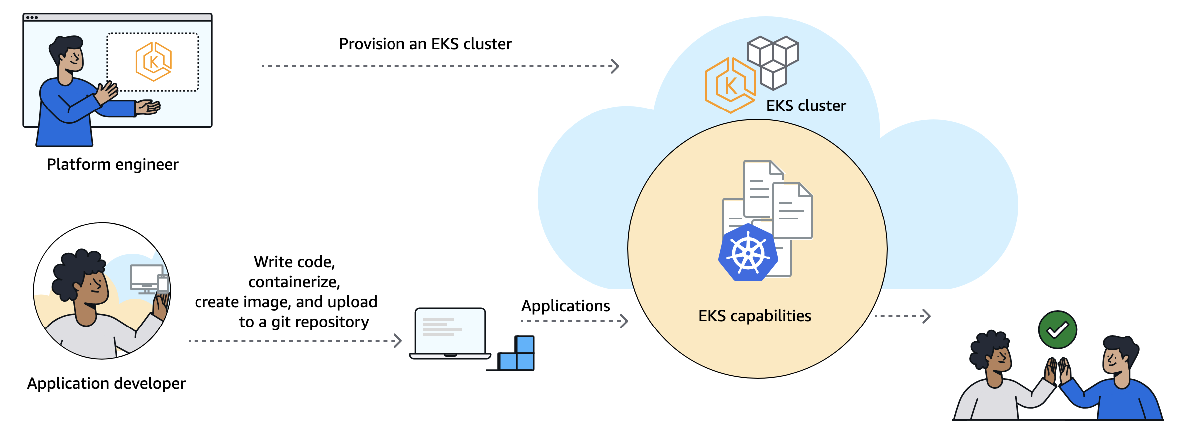
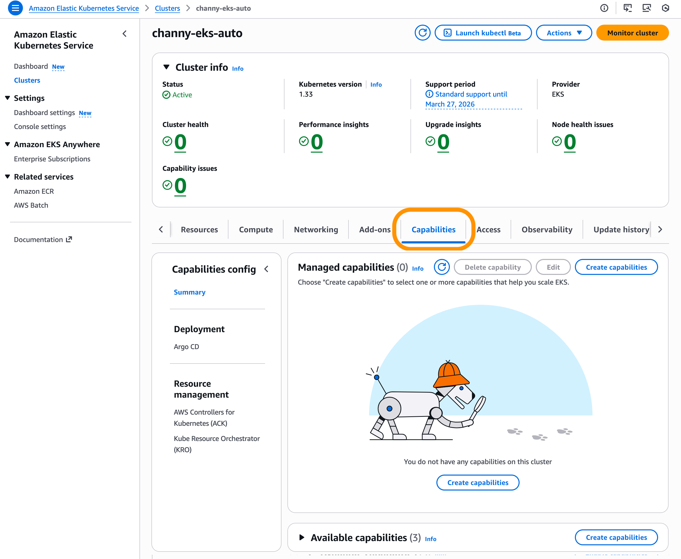
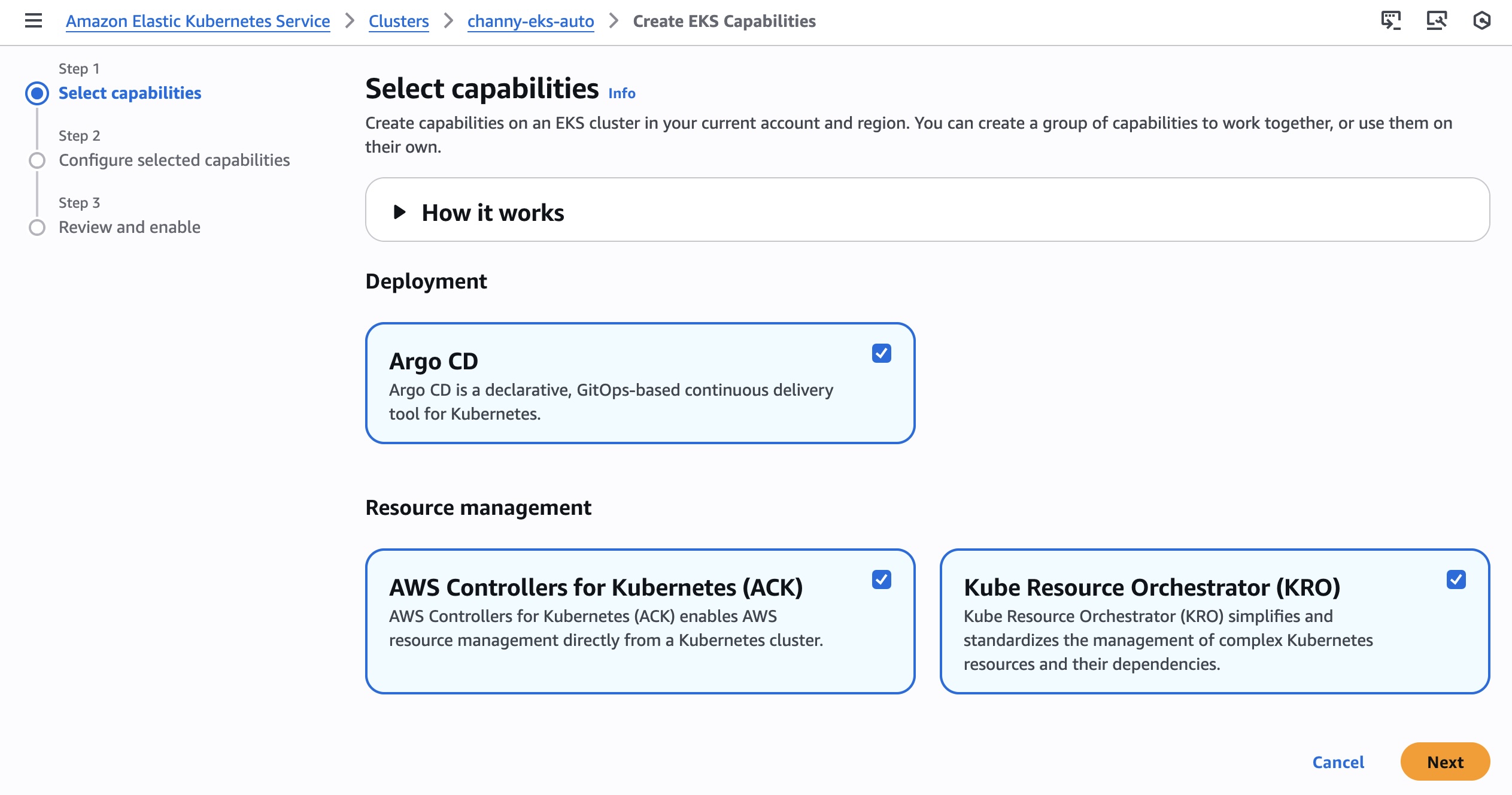
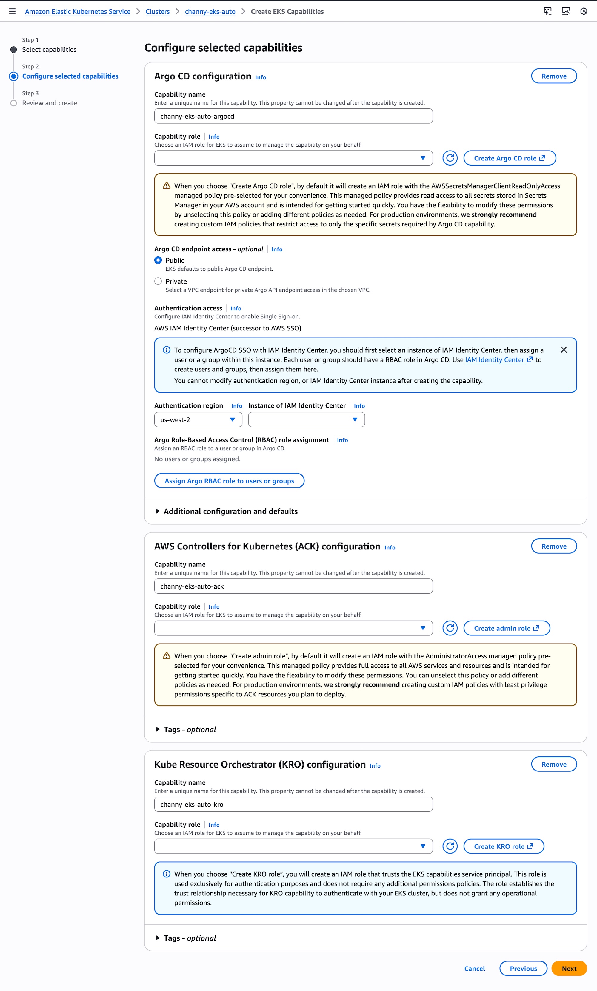
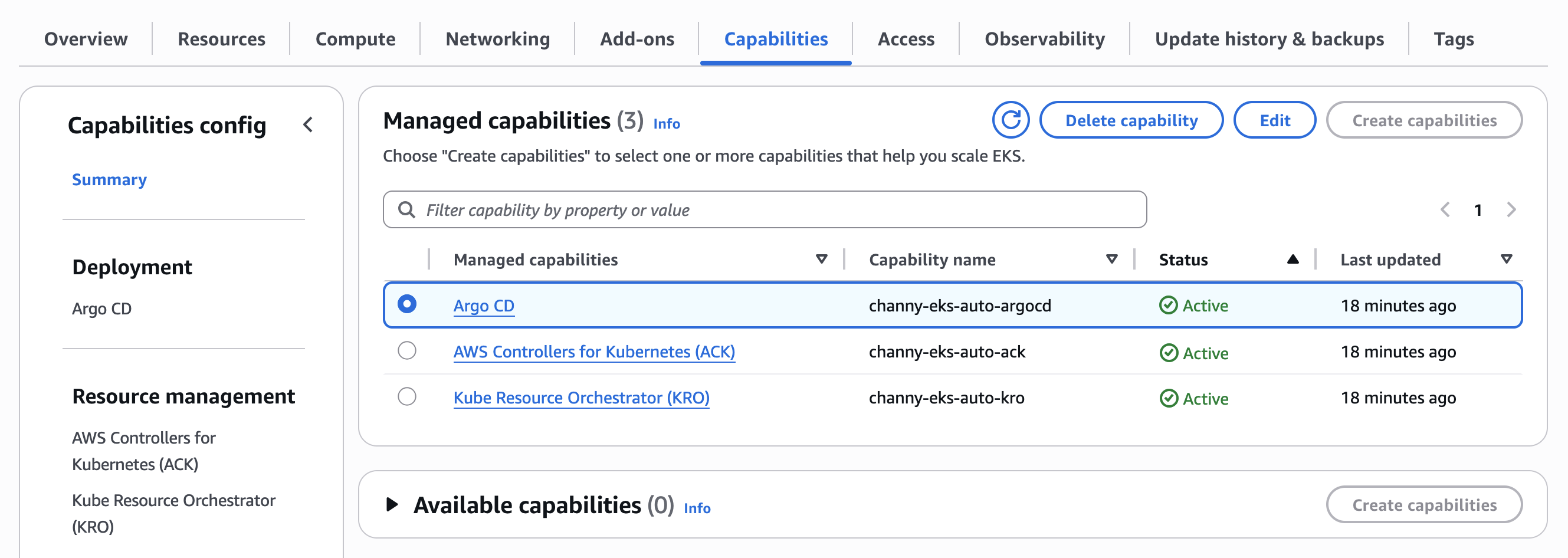
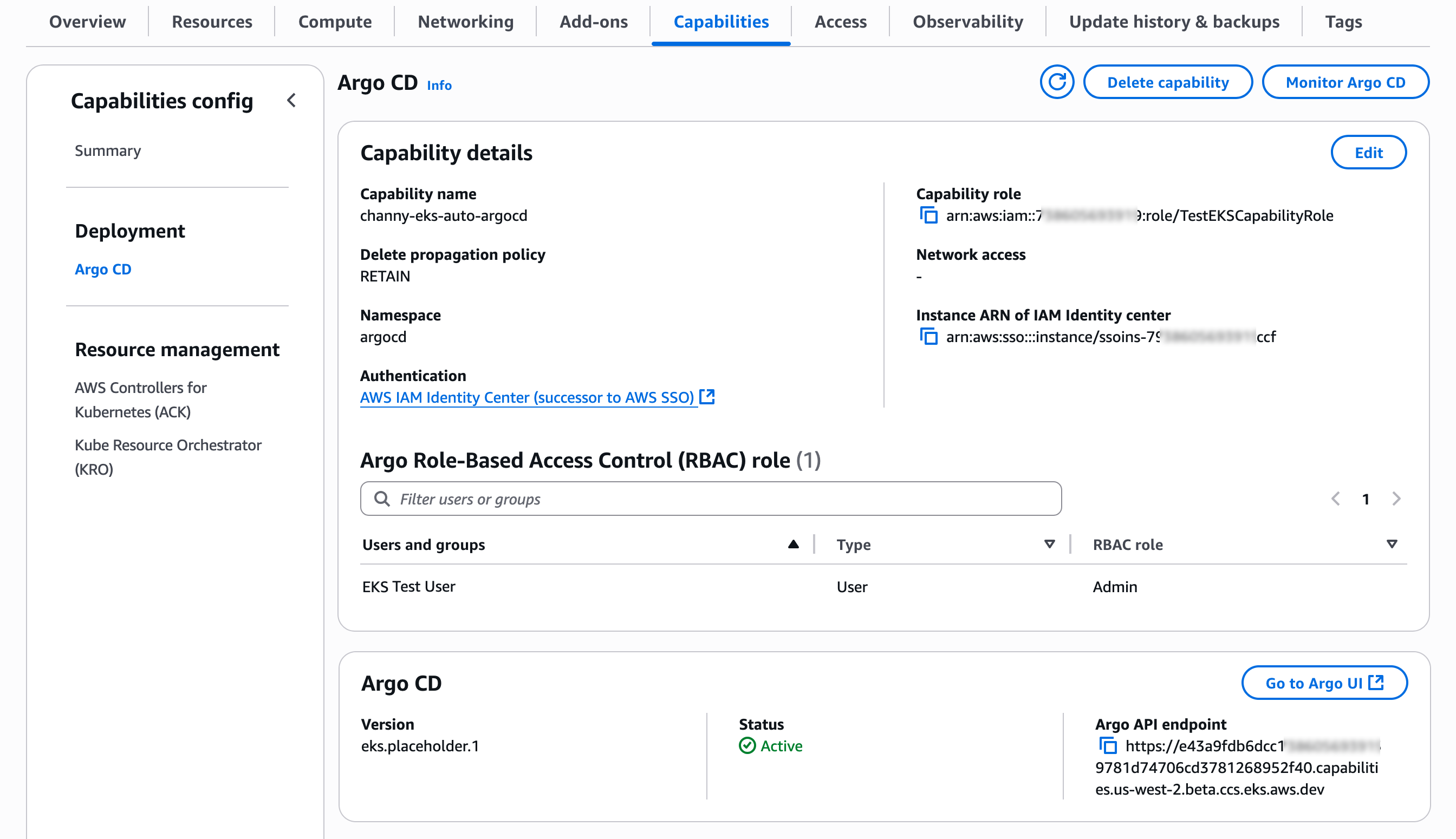
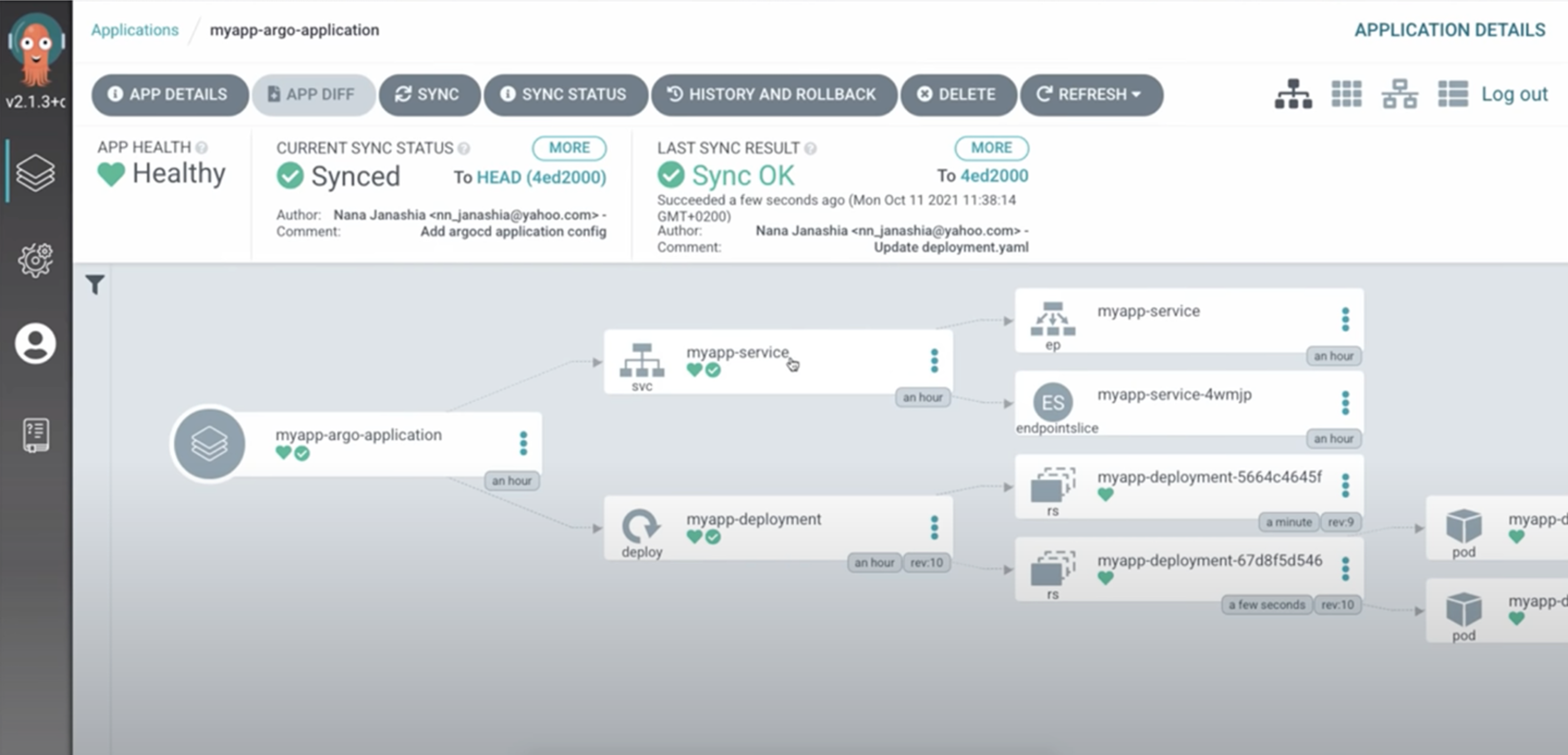


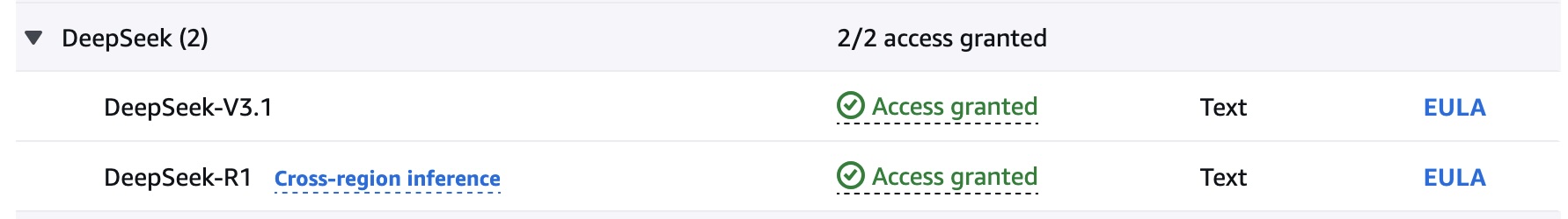
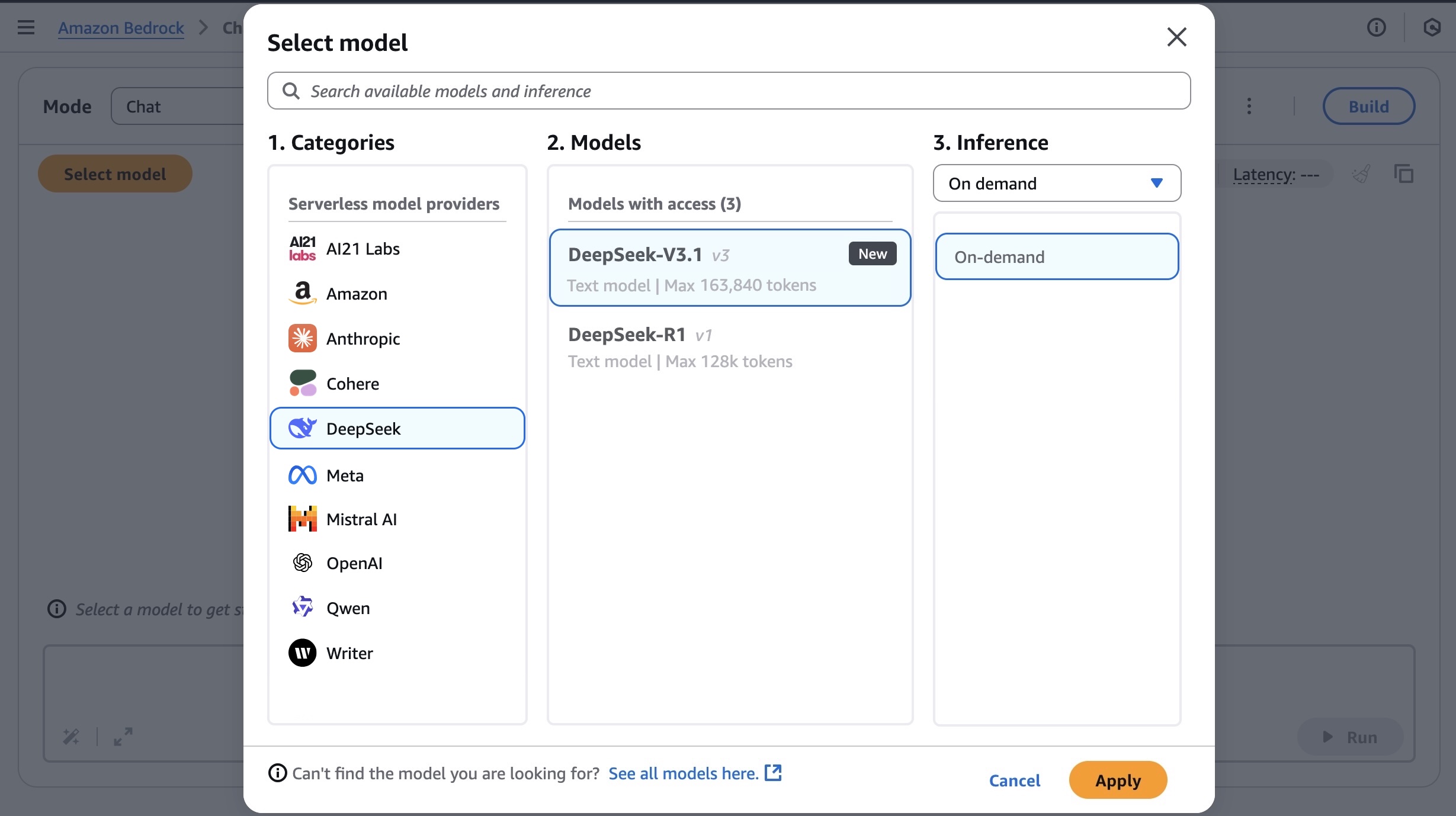
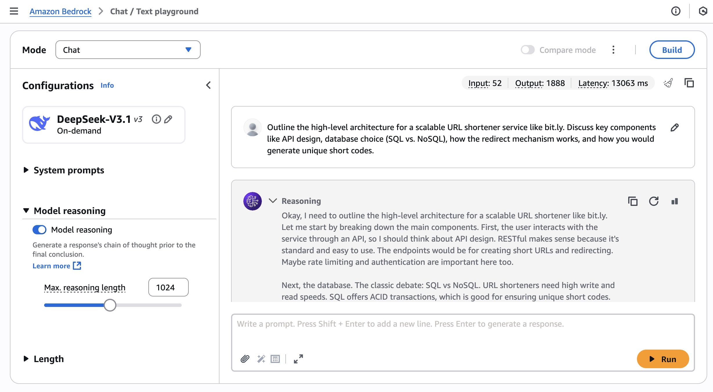
 Last week,
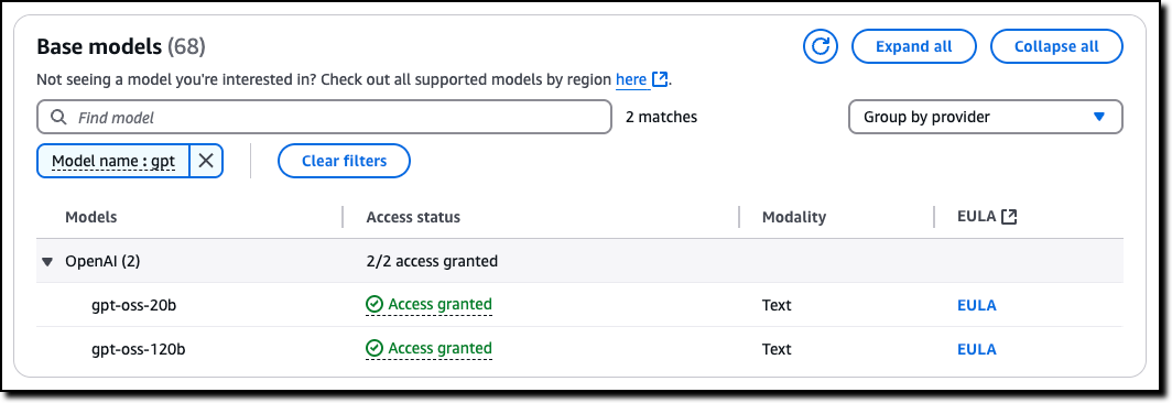
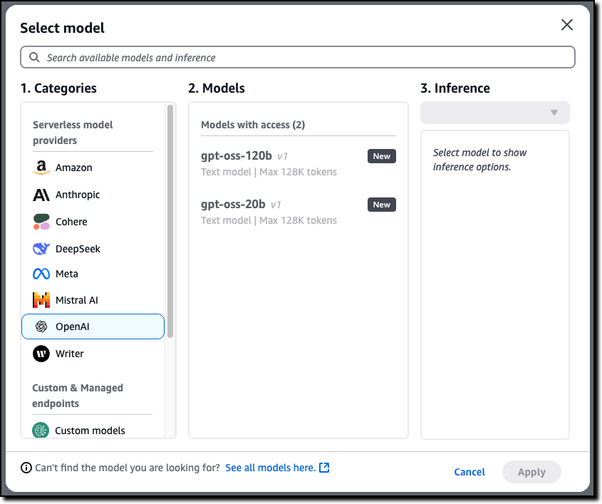
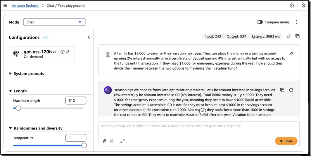
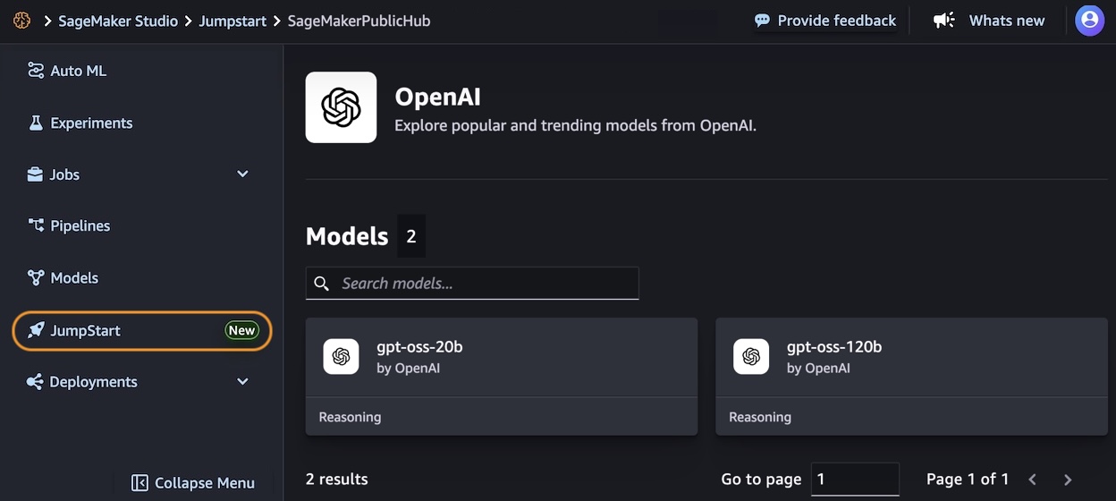
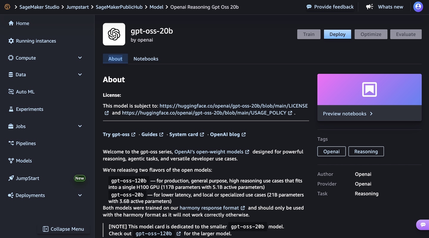


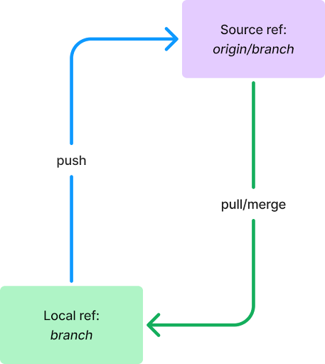

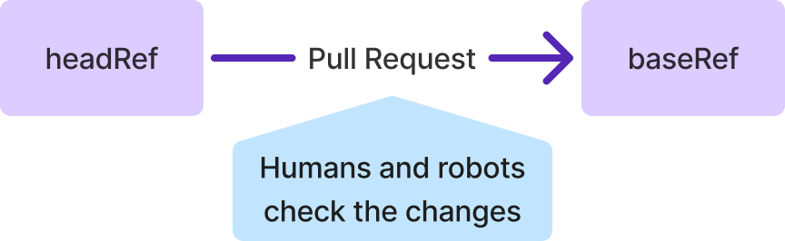
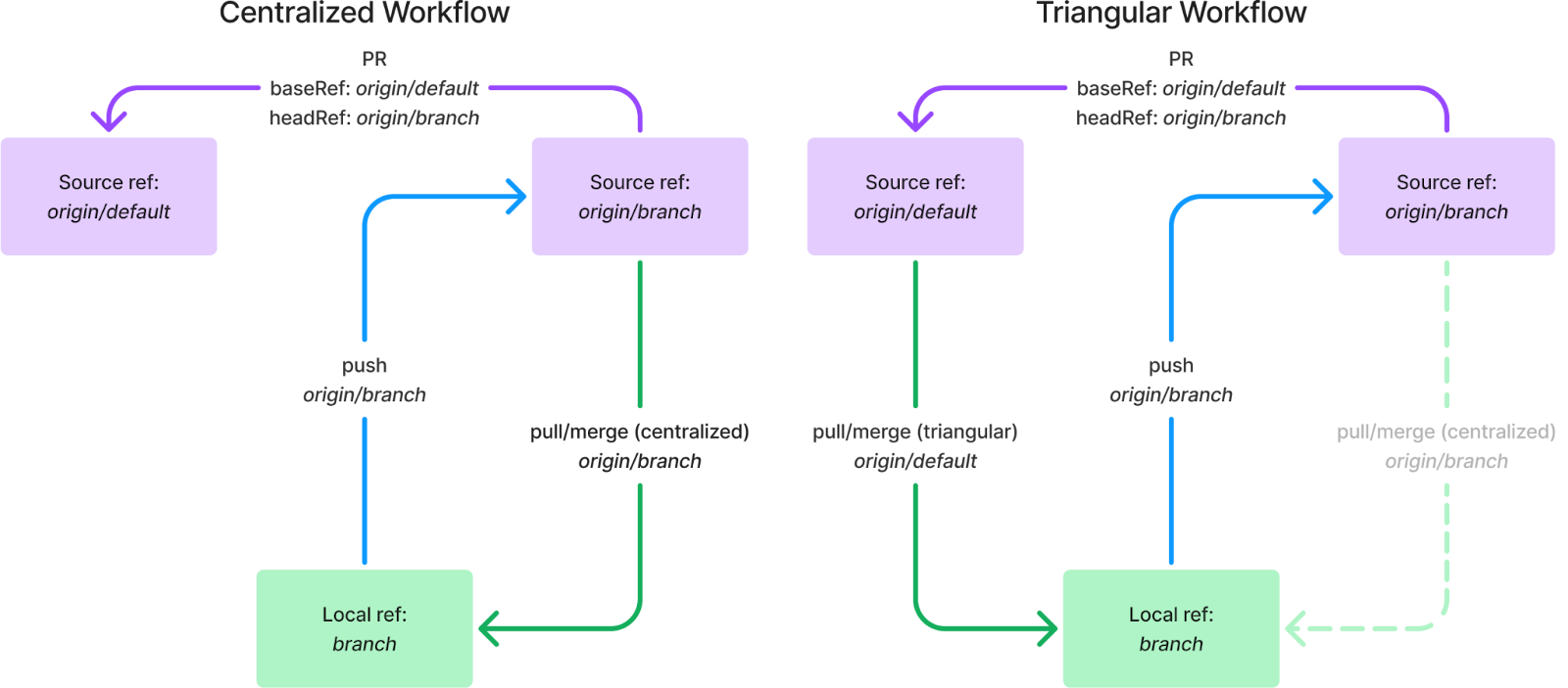
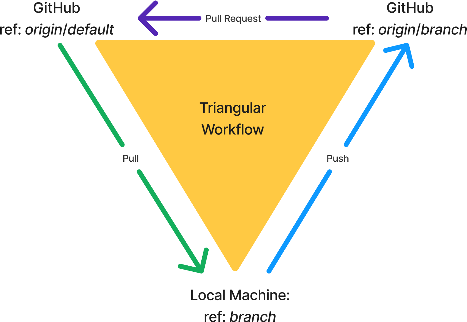
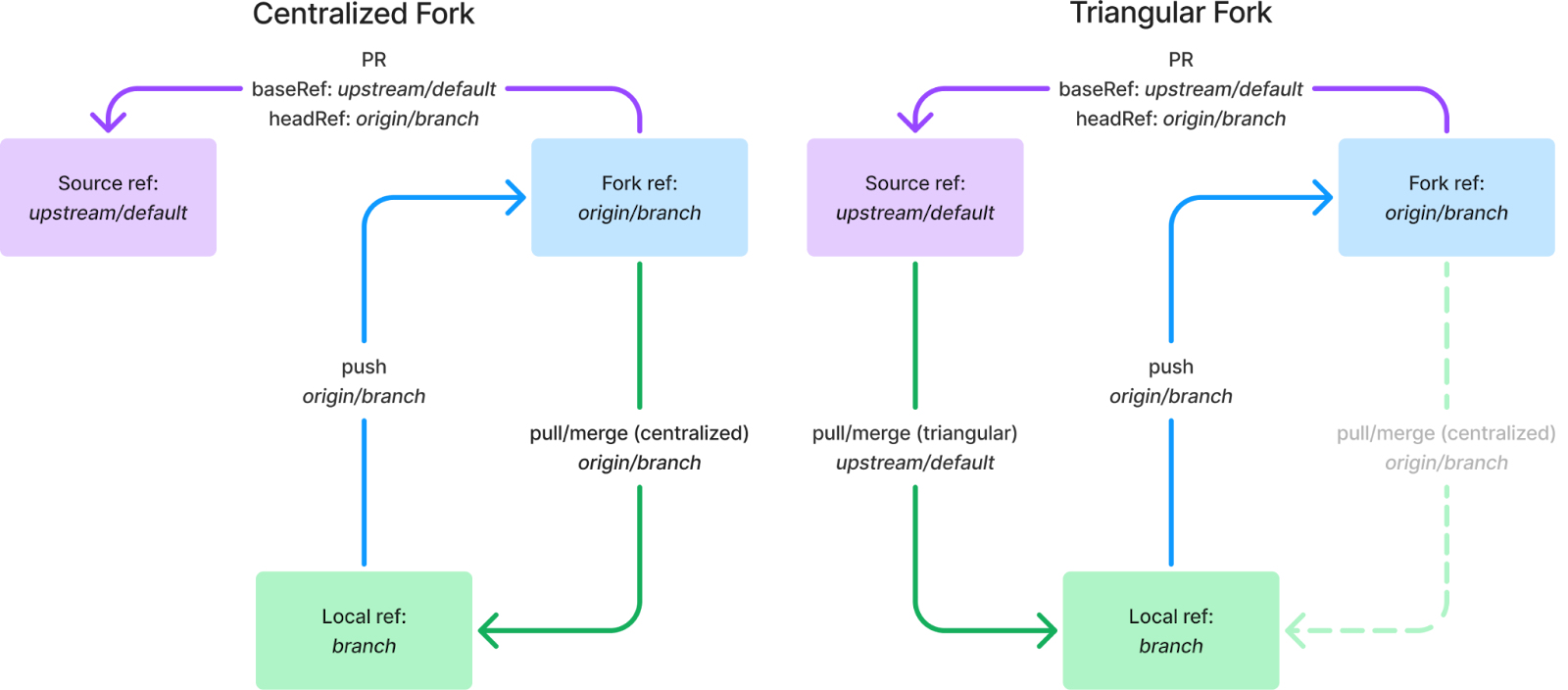
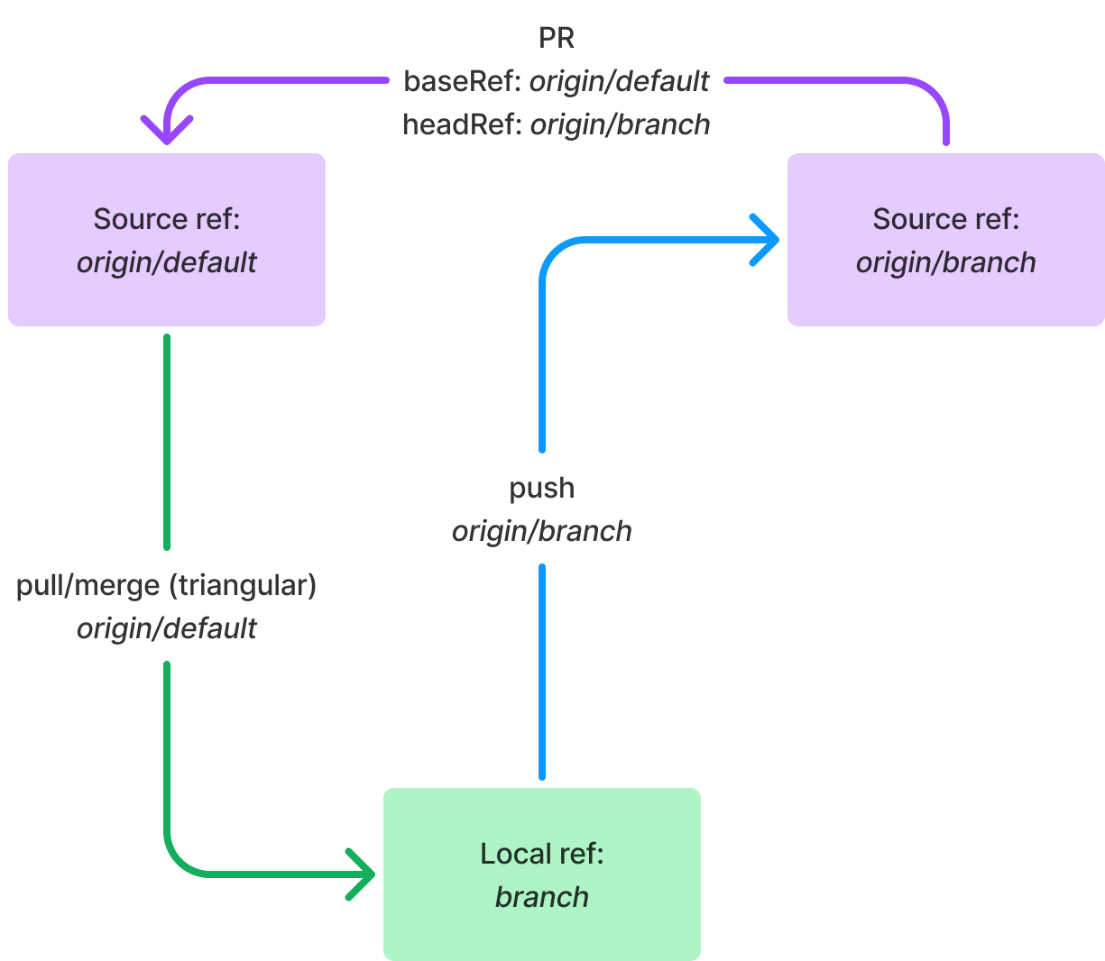
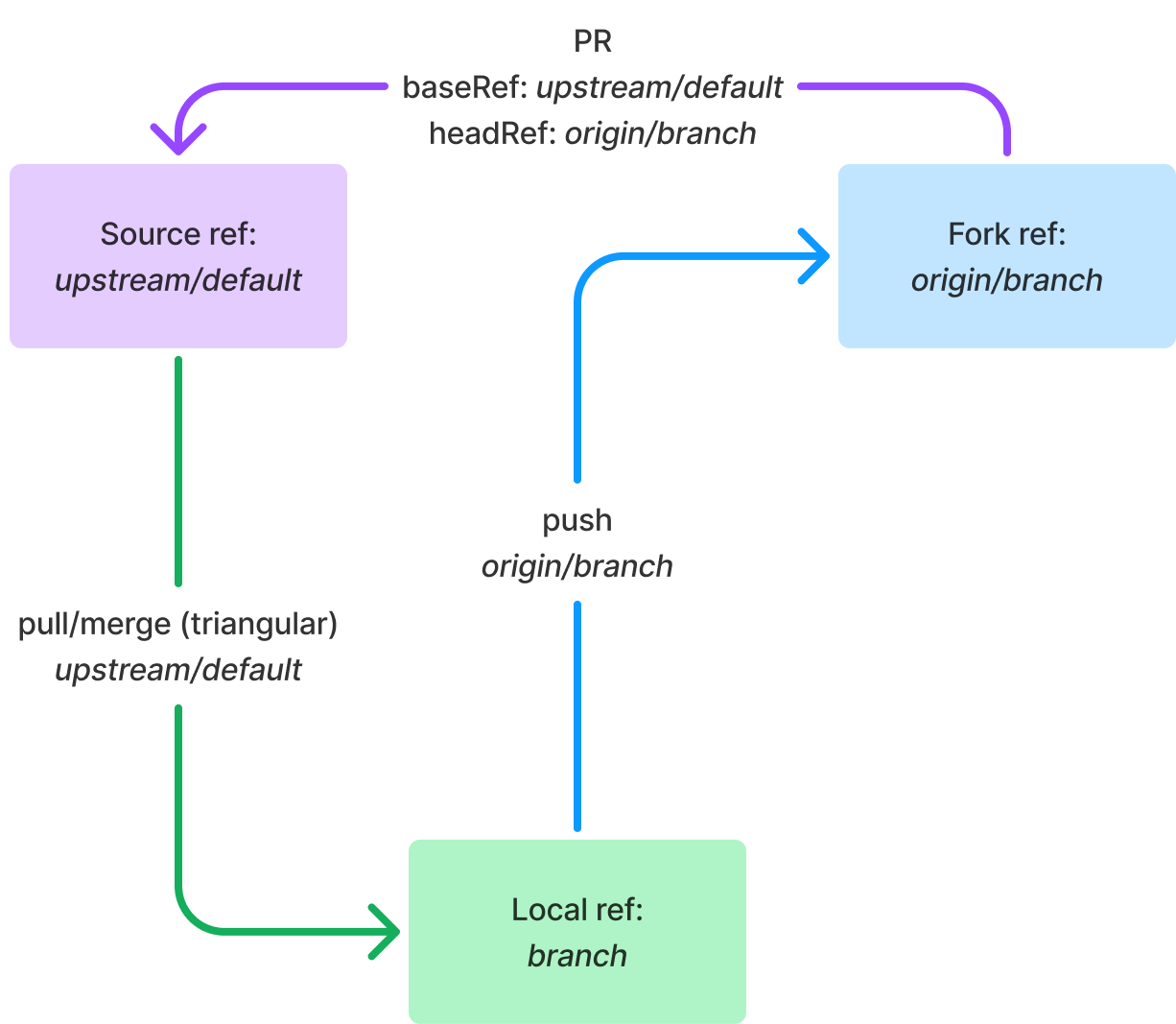

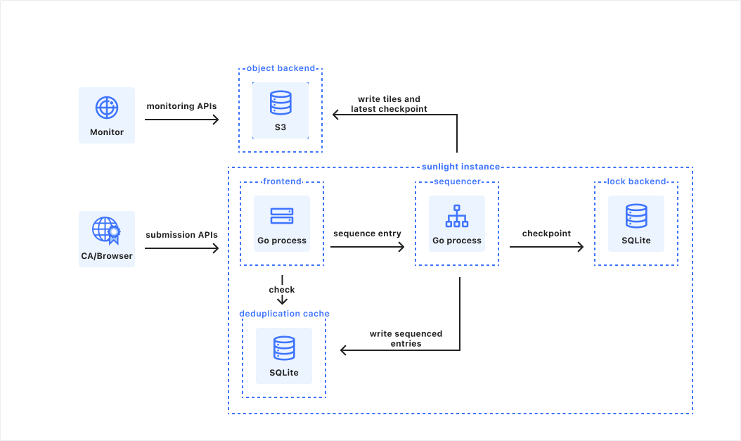
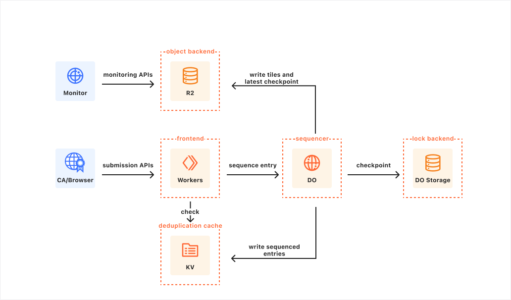
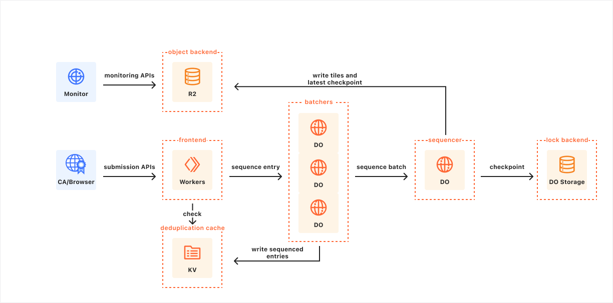


 Lorenzo Nicora works as Senior Streaming Solution Architect at AWS, helping customers across EMEA. He has been building cloud-centered, data-intensive systems for over 25 years, working across industries both through consultancies and product companies. He has used open-source technologies extensively and contributed to several projects, including Apache Flink, and is the maintainer of the Flink Prometheus connector.
 Francisco Morillo is a Senior Streaming Solutions Architect at AWS. Francisco works with AWS customers, helping them design real-time analytics architectures using AWS services, supporting Amazon MSK and Amazon Managed Service for Apache Flink. He is also a main contributor to the Flink Prometheus connector.
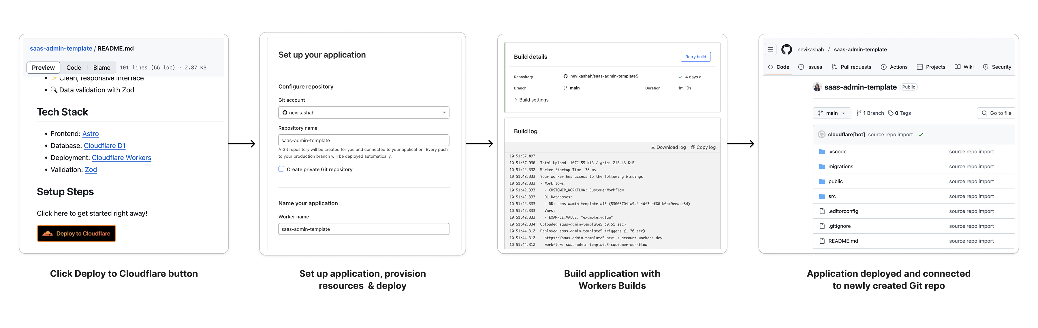

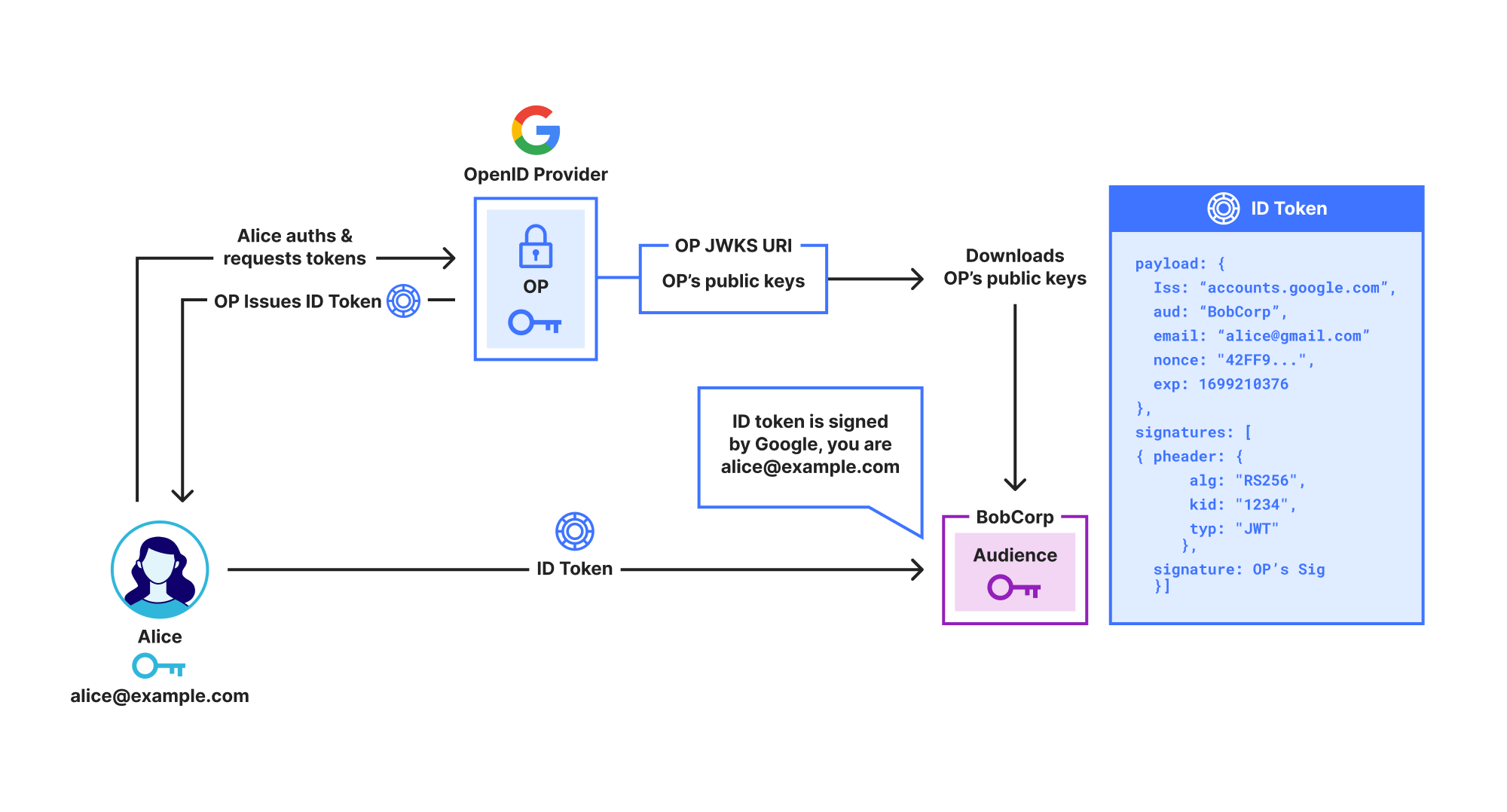
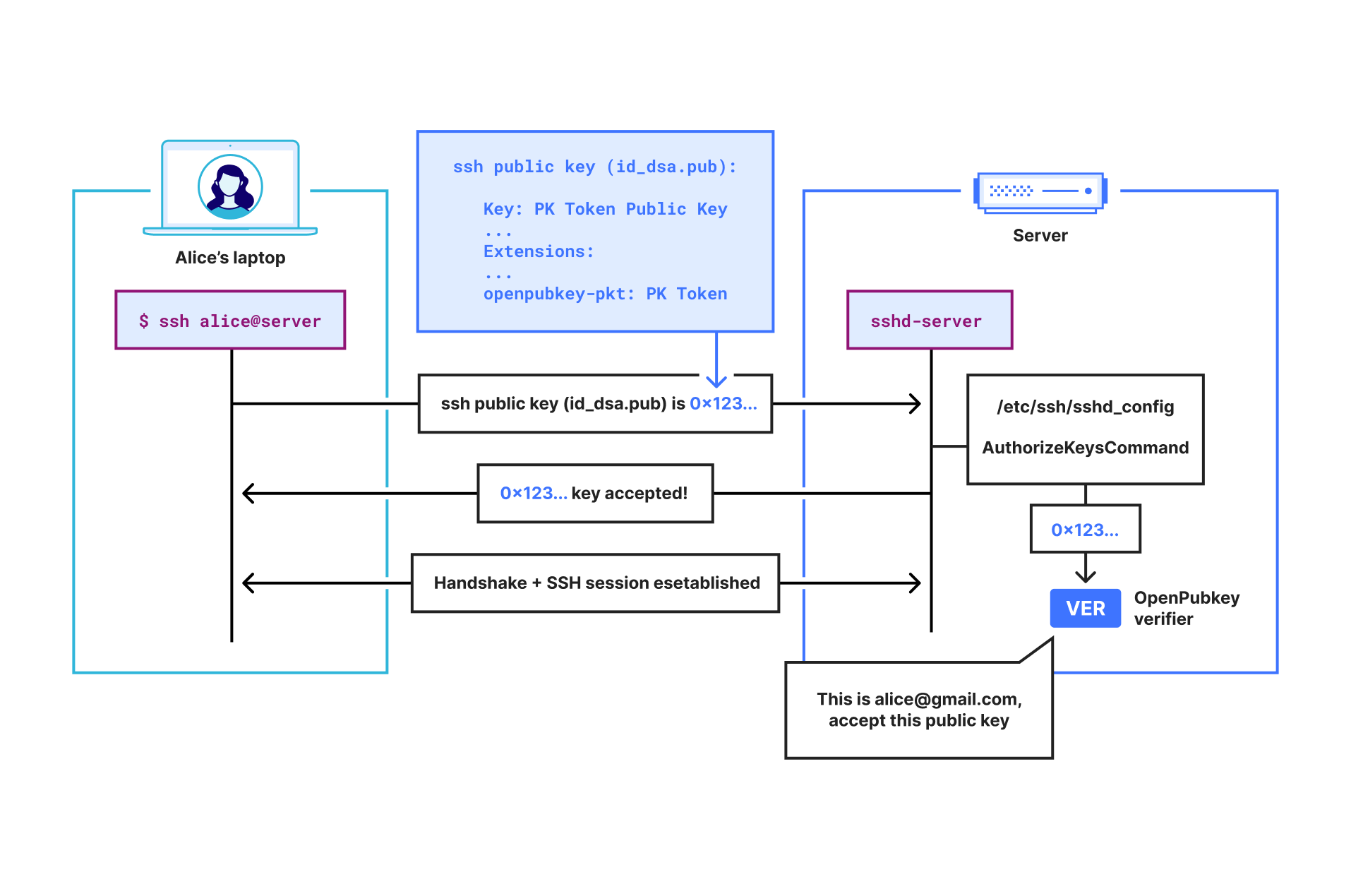


 Raj Ramasubbu is a Senior Analytics Specialist Solutions Architect focused on big data and analytics and AI/ML with Amazon Web Services. He helps customers architect and build highly scalable, performant, and secure cloud-based solutions on AWS. Raj provided technical expertise and leadership in building data engineering, big data analytics, business intelligence, and data science solutions for over 18 years prior to joining AWS. He helped customers in various industry verticals like healthcare, medical devices, life science, retail, asset management, car insurance, residential REIT, agriculture, title insurance, supply chain, document management, and real estate.
 Francisco Morillo is a Streaming Solutions Architect at AWS. Francisco works with AWS customers, helping them design real-time analytics architectures using AWS services, supporting Amazon Managed Streaming for Apache Kafka (Amazon MSK) and Amazon Managed Service for Apache Flink.
 Ismail Makhlouf is a Senior Specialist Solutions Architect for Data Analytics at AWS. Ismail focuses on architecting solutions for organizations across their end-to-end data analytics estate, including batch and real-time streaming, big data, data warehousing, and data lake workloads. He primarily partners with airlines, manufacturers, and retail organizations to support them to achieve their business objectives with well-architected data platforms.

