Post Syndicated from Constantin Pan original https://blog.cloudflare.com/how-we-make-sense-of-too-much-data/

Cloudflare’s network provides an enormous array of services to our customers. We collect and deliver associated data to customers in the form of event logs and aggregated analytics. As of December 2024, our data pipeline is ingesting up to 706M events per second generated by Cloudflare’s services, and that represents 100x growth since our 2018 data pipeline blog post. 

At peak, we are moving 107 GiB/s of compressed data, either pushing it directly to customers or subjecting it to additional queueing and batching.

All of these data streams power things like Logs, Analytics, and billing, as well as other products, such as training machine learning models for bot detection. This blog post is focused on techniques we use to efficiently and accurately deal with the high volume of data we ingest for our Analytics products. A previous blog post provides a deeper dive into the data pipeline for Logs. 

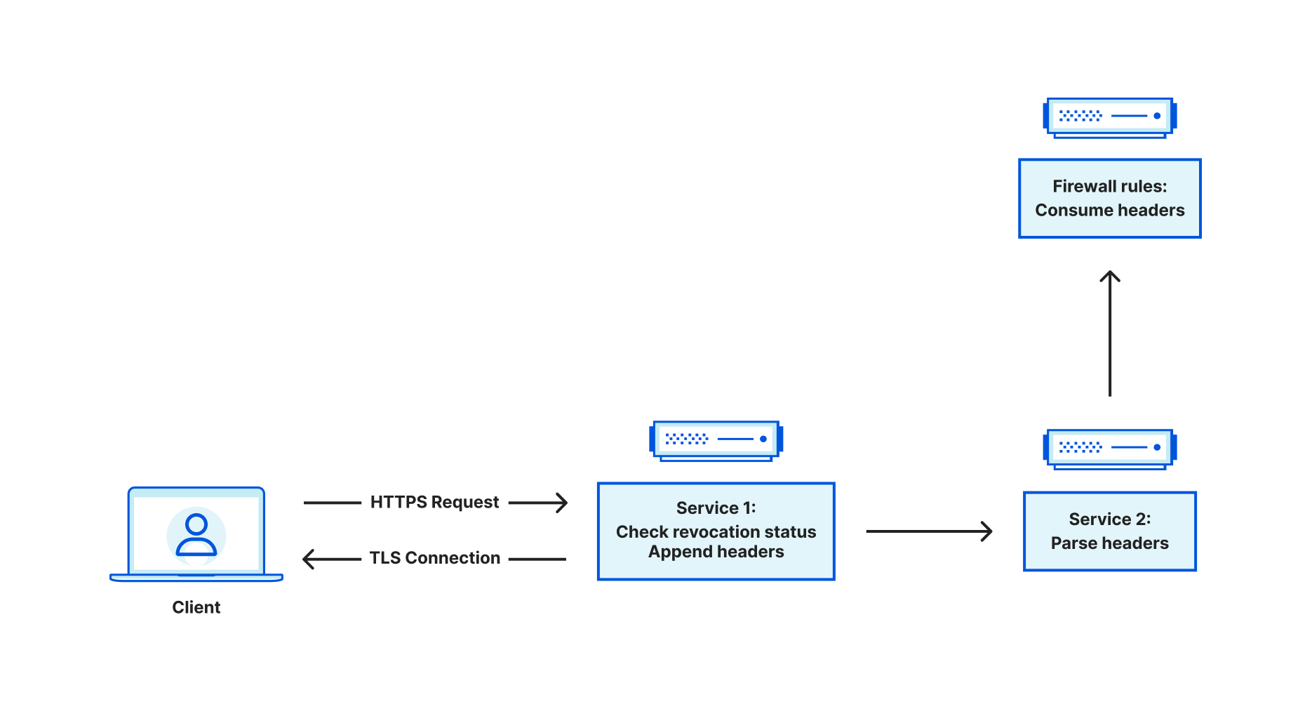
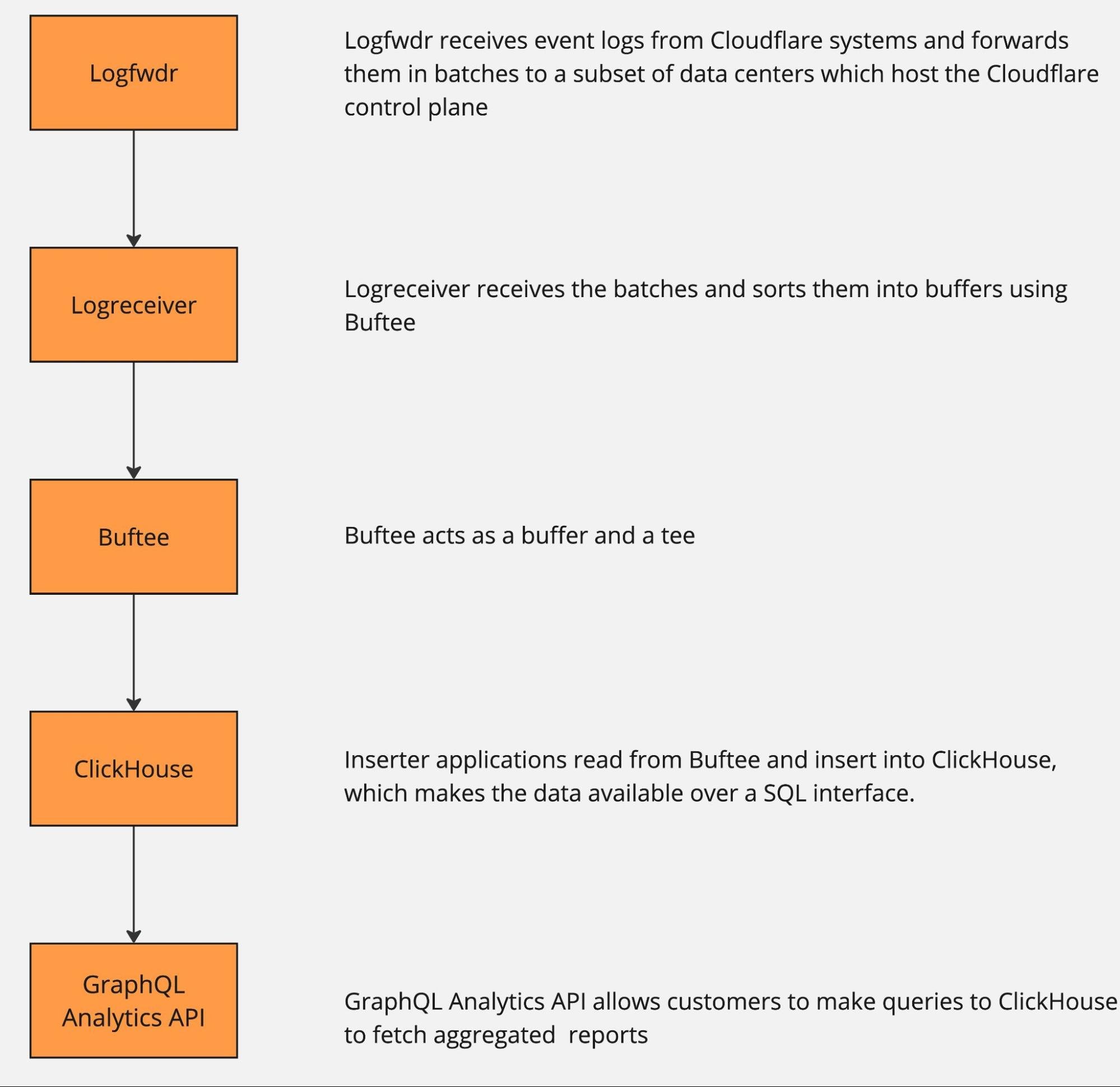
The pipeline can be roughly described by the following diagram.

The data pipeline has multiple stages, and each can and will naturally break or slow down because of hardware failures or misconfiguration. And when that happens, there is just too much data to be able to buffer it all for very long. Eventually some will get dropped, causing gaps in analytics and a degraded product experience unless proper mitigations are in place.

How does one retain valuable information from more than half a billion events per second, when some must be dropped? Drop it in a controlled way, by downsampling.

Here is a visual analogy showing the difference between uncontrolled data loss and downsampling. In both cases the same number of pixels were delivered. One is a higher resolution view of just a small portion of a popular painting, while the other shows the full painting, albeit blurry and highly pixelated.

As we noted above, any point in the pipeline can fail, so we want the ability to downsample at any point as needed. Some services proactively downsample data at the source before it even hits Logfwdr. This makes the information extracted from that data a little bit blurry, but much more useful than what otherwise would be delivered: random chunks of the original with gaps in between, or even nothing at all. The amount of “blur” is outside our control (we make our best effort to deliver full data), but there is a robust way to estimate it, as discussed in the next section.

Logfwdr can decide to downsample data sitting in the buffer when it overflows. Logfwdr handles many data streams at once, so we need to prioritize them by assigning each data stream a weight and then applying max-min fairness to better utilize the buffer. It allows each data stream to store as much as it needs, as long as the whole buffer is not saturated. Once it is saturated, streams divide it fairly according to their weighted size.

In our implementation (Go), each data stream is driven by a goroutine, and they cooperate via channels. They consult a single tracker object every time they allocate and deallocate memory. The tracker uses a max-heap to always know who the heaviest participant is and what the total usage is. Whenever the total usage goes over the limit, the tracker repeatedly sends the “please shed some load” signal to the heaviest participant, until the usage is again under the limit.

The effect of this is that healthy streams, which buffer a tiny amount, allocate whatever they need without losses. But any lagging streams split the remaining memory allowance fairly.

We downsample more or less uniformly, by always taking some of the least downsampled batches from the buffer (using min-heap to find those) and merging them together upon downsampling.

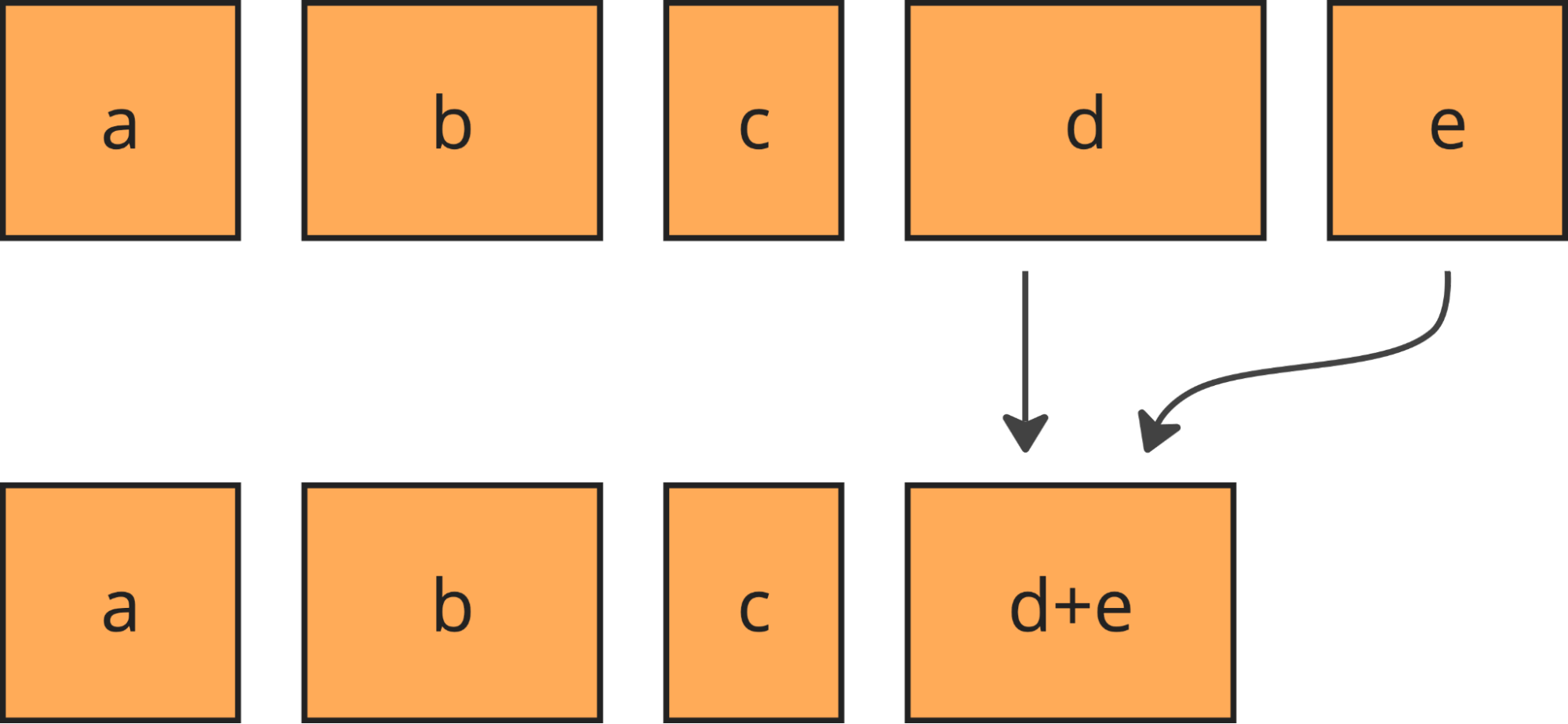
^{Merging keeps the batches roughly the same size and their number under control.}

Downsampling is cheap, but since data in the buffer is compressed, it causes recompression, which is the single most expensive thing we do to the data. But using extra CPU time is the last thing you want to do when the system is under heavy load! We compensate for the recompression costs by starting to downsample the fresh data as well (before it gets compressed for the first time) whenever the stream is in the “shed the load” state.

We called this approach “bottomless buffers”, because you can squeeze effectively infinite amounts of data in there, and it will just automatically be thinned out. Bottomless buffers resemble reservoir sampling, where the buffer is the reservoir and the population comes as the input stream. But there are some differences. First is that in our pipeline the input stream of data never ends, while reservoir sampling assumes it ends to finalize the sample. Secondly, the resulting sample also never ends.

Let’s look at the next stage in the pipeline: Logreceiver. It sits in front of a distributed queue. The purpose of logreceiver is to partition each stream of data by a key that makes it easier for Logpush, Analytics inserters, or some other process to consume.

Logreceiver proactively performs adaptive sampling of analytics. This improves the accuracy of analytics for small customers (receiving on the order of 10 events per day), while more aggressively downsampling large customers (millions of events per second). Logreceiver then pushes the same data at multiple resolutions (100%, 10%, 1%, etc.) into different topics in the distributed queue. This allows it to keep pushing something rather than nothing when the queue is overloaded, by just skipping writing the high-resolution samples of data.

The same goes for Inserters: they can skip reading or writing high-resolution data. The Analytics APIs can skip reading high resolution data. The analytical database might be unable to read high resolution data because of overload or degraded cluster state or because there is just too much to read (very wide time range or very large customer). Adaptively dropping to lower resolutions allows the APIs to return some results in all of those cases.

Okay, we have some downsampled data in the analytical database. It looks like the original data, but with some rows missing. How do we make sense of it? How do we know if the results can be trusted?

Let’s look at the math.

Since the amount of sampling can vary over time and between nodes in the distributed system, we need to store this information along with the data. With each event $x_i$ we store its sample interval, which is the reciprocal to its inclusion probability $\pi_i = \frac{1}{\text{sample interval}}$. For example, if we sample 1 in every 1,000 events, each of the events included in the resulting sample will have its $\pi_i = 0.001$, so the sample interval will be 1,000. When we further downsample that batch of data, the inclusion probabilities (and the sample intervals) multiply together: a 1 in 1,000 sample from a 1 in 1,000 sample is a 1 in 1,000,000 sample of the original population. The sample interval of an event can also be interpreted roughly as the number of original events that this event represents, so in the literature it is known as weight $w_i = \frac{1}{\pi_i}$.

We rely on the Horvitz-Thompson estimator (HT, paper) in order to derive analytics about $x_i$. It gives two estimates: the analytical estimate (e.g. the population total or size) and the estimate of the variance of that estimate. The latter enables us to figure out how accurate the results are by building confidence intervals. They define ranges that cover the true value with a given probability (confidence level). A typical confidence level is 0.95, at which a confidence interval (a, b) tells that you can be 95% sure the true SUM or COUNT is between a and b.

So far, we know how to use the HT estimator for doing SUM, COUNT, and AVG.

Given a sample of size $n$, consisting of values $x_i$ and their inclusion probabilities $\pi_i$, the HT estimator for the population total (i.e. SUM) would be

$$\widehat{T}=\sum_{i=1}^n{\frac{x_i}{\pi_i}}=\sum_{i=1}^n{x_i w_i}.$$

The variance of $\widehat{T}$ is:

$$\widehat{V}(\widehat{T}) = \sum_{i=1}^n{x_i^2 \frac{1 – \pi_i}{\pi_i^2}} + \sum_{i \neq j}^n{x_i x_j \frac{\pi_{ij} – \pi_i \pi_j}{\pi_{ij} \pi_i \pi_j}},$$

where $\pi_{ij}$ is the probability of both $i$-th and $j$-th events being sampled together.

We use Poisson sampling, where each event is subjected to an independent Bernoulli trial (“coin toss”) which determines whether the event becomes part of the sample. Since each trial is independent, we can equate $\pi_{ij} = \pi_i \pi_j$, which when plugged in the variance estimator above turns the right-hand sum to zero:

$$\widehat{V}(\widehat{T}) = \sum_{i=1}^n{x_i^2 \frac{1 – \pi_i}{\pi_i^2}} + \sum_{i \neq j}^n{x_i x_j \frac{0}{\pi_{ij} \pi_i \pi_j}},$$

thus

$$\widehat{V}(\widehat{T}) = \sum_{i=1}^n{x_i^2 \frac{1 – \pi_i}{\pi_i^2}} = \sum_{i=1}^n{x_i^2 w_i (w_i-1)}.$$

For COUNT we use the same estimator, but plug in $x_i = 1$. This gives us:

$$\begin{align}
\widehat{C} &= \sum_{i=1}^n{\frac{1}{\pi_i}} = \sum_{i=1}^n{w_i},\\
\widehat{V}(\widehat{C}) &= \sum_{i=1}^n{\frac{1 – \pi_i}{\pi_i^2}} = \sum_{i=1}^n{w_i (w_i-1)}.
\end{align}$$

For AVG we would use

$$\begin{align}
\widehat{\mu} &= \frac{\widehat{T}}{N},\\
\widehat{V}(\widehat{\mu}) &= \frac{\widehat{V}(\widehat{T})}{N^2},
\end{align}$$

if we could, but the original population size $N$ is not known, it is not stored anywhere, and it is not even possible to store because of custom filtering at query time. Plugging $\widehat{C}$ instead of $N$ only partially works. It gives a valid estimator for the mean itself, but not for its variance, so the constructed confidence intervals are unusable.

In all cases the corresponding pair of estimates are used as the $\mu$ and $\sigma^2$ of the normal distribution (because of the central limit theorem), and then the bounds for the confidence interval (of confidence level ) are:

$$\Big( \mu – \Phi^{-1}\big(\frac{1 + \alpha}{2}\big) \cdot \sigma, \quad \mu + \Phi^{-1}\big(\frac{1 + \alpha}{2}\big) \cdot \sigma\Big).$$

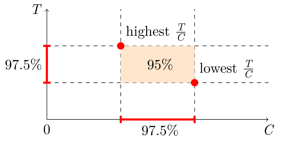
We do not know the N, but there is a workaround: simultaneous confidence intervals. Construct confidence intervals for SUM and COUNT independently, and then combine them into a confidence interval for AVG. This is known as the Bonferroni method. It requires generating wider (half the “inconfidence”) intervals for SUM and COUNT. Here is a simplified visual representation, but the actual estimator will have to take into account the possibility of the orange area going below zero.

In SQL, the estimators and confidence intervals look like this:

WITH sum(x * _sample_interval)                              AS t,
     sum(x * x * _sample_interval * (_sample_interval - 1)) AS vt,
     sum(_sample_interval)                                  AS c,
     sum(_sample_interval * (_sample_interval - 1))         AS vc,
     -- ClickHouse does not expose the erf⁻¹ function, so we precompute some magic numbers,
     -- (only for 95% confidence, will be different otherwise):
     --   1.959963984540054 = Φ⁻¹((1+0.950)/2) = √2 * erf⁻¹(0.950)
     --   2.241402727604945 = Φ⁻¹((1+0.975)/2) = √2 * erf⁻¹(0.975)
     1.959963984540054 * sqrt(vt) AS err950_t,
     1.959963984540054 * sqrt(vc) AS err950_c,
     2.241402727604945 * sqrt(vt) AS err975_t,
     2.241402727604945 * sqrt(vc) AS err975_c
SELECT t - err950_t AS lo_total,
       t            AS est_total,
       t + err950_t AS hi_total,
       c - err950_c AS lo_count,
       c            AS est_count,
       c + err950_c AS hi_count,
       (t - err975_t) / (c + err975_c) AS lo_average,
       t / c                           AS est_average,
       (t + err975_t) / (c - err975_c) AS hi_average
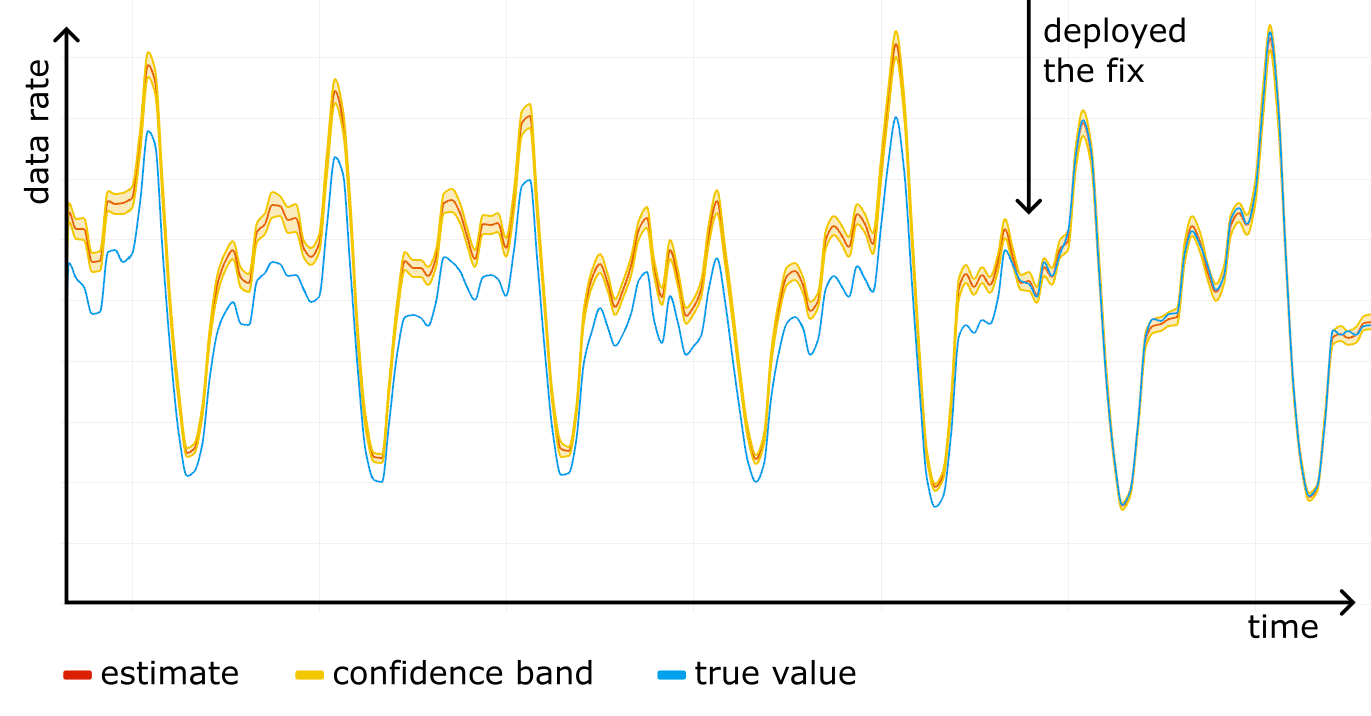
FROM ...

Construct a confidence interval for each timeslot on the timeseries, and you get a confidence band, clearly showing the accuracy of the analytics. The figure below shows an example of such a band in shading around the line.

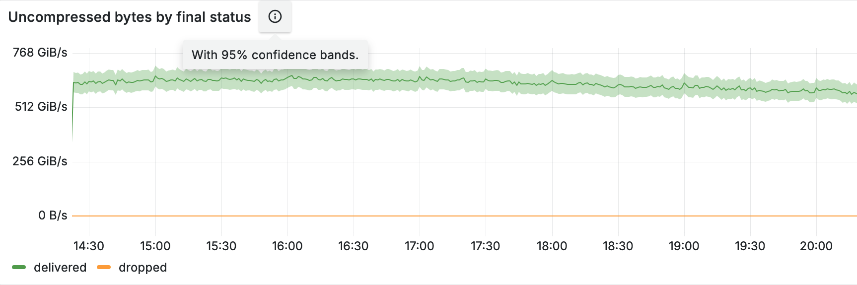
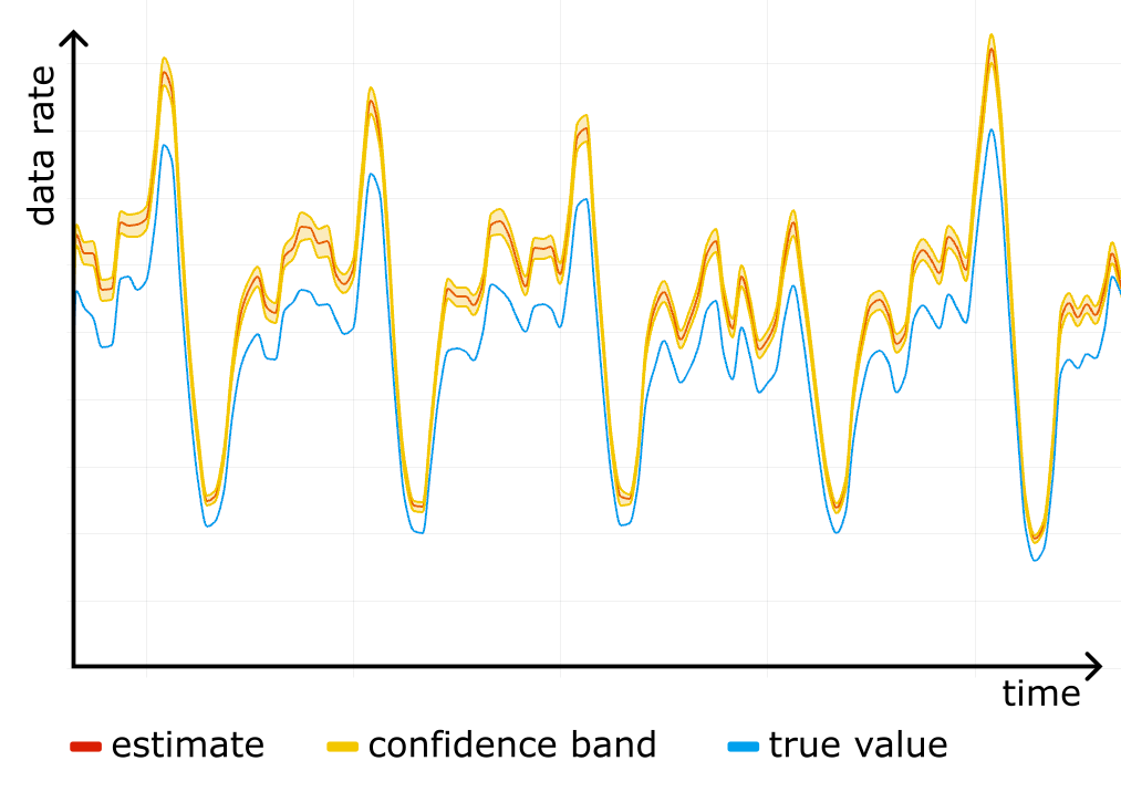
We started using confidence bands on our internal dashboards, and after a while noticed something scary: a systematic error! For one particular website the “total bytes served” estimate was higher than the true control value obtained from rollups, and the confidence bands were way off. See the figure below, where the true value (blue line) is outside the yellow confidence band at all times.

We checked the stored data for corruption, it was fine. We checked the math in the queries, it was fine. It was only after reading through the source code for all of the systems responsible for sampling that we found a candidate for the root cause.

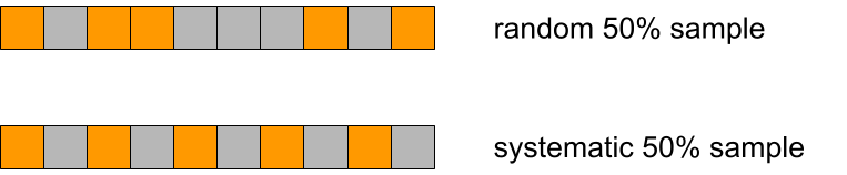
We used simple random sampling everywhere, basically “tossing a coin” for each event, but in Logreceiver sampling was done differently. Instead of sampling randomly it would perform systematic sampling by picking events at equal intervals starting from the first one in the batch.

Why would that be a problem?

There are two reasons. The first is that we can no longer claim $\pi_{ij} = \pi_i \pi_j$, so the simplified variance estimator stops working and confidence intervals cannot be trusted. But even worse, the estimator for the total becomes biased. To understand why exactly, we wrote a short repro code in Python:

import itertools

def take_every(src, period):
    for i, x in enumerate(src):
    if i % period == 0:
        yield x

pattern = [10, 1, 1, 1, 1, 1]
sample_interval = 10 # bad if it has common factors with len(pattern)
true_mean = sum(pattern) / len(pattern)

orig = itertools.cycle(pattern)
sample_size = 10000
sample = itertools.islice(take_every(orig, sample_interval), sample_size)

sample_mean = sum(sample) / sample_size

print(f"{true_mean=} {sample_mean=}")

After playing with different values for pattern and sample_interval in the code above, we realized where the bias was coming from.

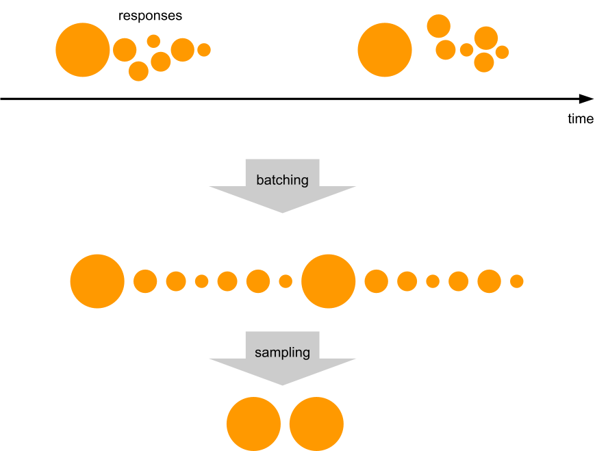
Imagine a person opening a huge generated HTML page with many small/cached resources, such as icons. The first response will be big, immediately followed by a burst of small responses. If the website is not visited that much, responses will tend to end up all together at the start of a batch in Logfwdr. Logreceiver does not cut batches, only concatenates them. The first response remains first, so it always gets picked and skews the estimate up.

We checked the hypothesis against the raw unsampled data that we happened to have because that particular website was also using one of the Logs products. We took all events in a given time range, and grouped them by cutting at gaps of at least one minute. In each group, we ranked all events by time and looked at the variable of interest (response size in bytes), and put it on a scatter plot against the rank inside the group.

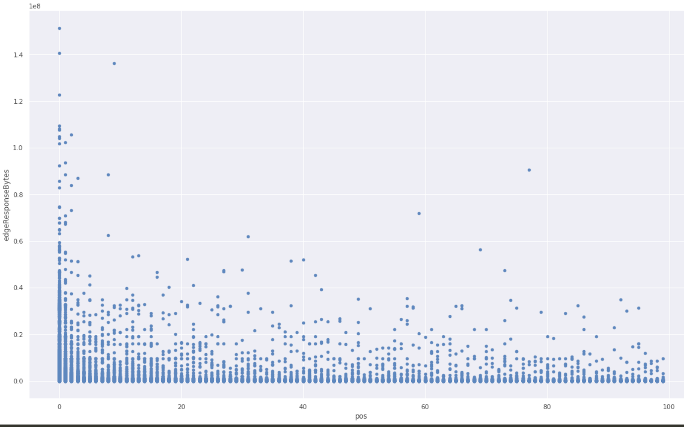
A clear pattern! The first response is much more likely to be larger than average.

We fixed the issue by making Logreceiver shuffle the data before sampling. As we rolled out the fix, the estimation and the true value converged.

Now, after battle testing it for a while, we are confident the HT estimator is implemented properly and we are using the correct sampling process.

We already power most of our analytics datasets with sampled data. For example, the Workers Analytics Engine exposes the sample interval in SQL, allowing our customers to build their own dashboards with confidence bands. In the GraphQL API, all of the data nodes that have “Adaptive” in their name are based on sampled data, and the sample interval is exposed as a field there as well, though it is not possible to build confidence intervals from that alone. We are working on exposing confidence intervals in the GraphQL API, and as an experiment have added them to the count and edgeResponseBytes (sum) fields on the httpRequestsAdaptiveGroups nodes. This is available under confidence(level: X).

Here is a sample GraphQL query:

query HTTPRequestsWithConfidence(
  $accountTag: string
  $zoneTag: string
  $datetimeStart: string
  $datetimeEnd: string
) {
  viewer {
    zones(filter: { zoneTag: $zoneTag }) {
      httpRequestsAdaptiveGroups(
        filter: {
          datetime_geq: $datetimeStart
          datetime_leq: $datetimeEnd
      }
      limit: 100
    ) {
      confidence(level: 0.95) {
        level
        count {
          estimate
          lower
          upper
          sampleSize
        }
        sum {
          edgeResponseBytes {
            estimate
            lower
            upper
            sampleSize
          }
        }
      }
    }
  }
}

The query above asks for the estimates and the 95% confidence intervals for SUM(edgeResponseBytes) and COUNT. The results will also show the sample size, which is good to know, as we rely on the central limit theorem to build the confidence intervals, thus small samples don’t work very well.

Here is the response from this query:

{
  "data": {
    "viewer": {
      "zones": [
        {
          "httpRequestsAdaptiveGroups": [
            {
              "confidence": {
                "level": 0.95,
                "count": {
                  "estimate": 96947,
                  "lower": "96874.24",
                  "upper": "97019.76",
                  "sampleSize": 96294
                },
                "sum": {
                  "edgeResponseBytes": {
                    "estimate": 495797559,
                    "lower": "495262898.54",
                    "upper": "496332219.46",
                    "sampleSize": 96294
                  }
                }
              }
            }
          ]
        }
      ]
    }
  },
  "errors": null
}

The response shows the estimated count is 96947, and we are 95% confident that the true count lies in the range 96874.24 to 97019.76. Similarly, the estimate and range for the sum of response bytes are provided.

The estimates are based on a sample size of 96294 rows, which is plenty of samples to calculate good confidence intervals.

We have discussed what kept our data pipeline scalable and resilient despite doubling in size every 1.5 years, how the math works, and how it is easy to mess up. We are constantly working on better ways to keep the data pipeline, and the products based on it, useful to our customers. If you are interested in doing things like that and want to help us build a better Internet, check out our careers page.