Post Syndicated from Kartik Kannapur original https://aws.amazon.com/blogs/big-data/data-preprocessing-for-machine-learning-on-amazon-emr-made-easy-with-aws-glue-databrew/
The machine learning (ML) lifecycle consists of several key phases: data collection, data preparation, feature engineering, model training, model evaluation, and model deployment. The data preparation and feature engineering phases ensure an ML model is given high-quality data that is relevant to the model’s purpose. Because most raw datasets require multiple cleaning steps (such as addressing missing values and imbalanced data) and numerous data transformations to produce useful features ready for model training, these phases are often considered the most time-consuming in the ML lifecycle. Additionally, producing well-prepared training datasets has typically required extensive knowledge of multiple data analysis libraries and frameworks. This has presented a barrier to entry for new ML practitioners and reduced iteration speed for more experienced practitioners.
In this post, we show you how to address this challenge with the newly released AWS Glue DataBrew. DataBrew is a visual data preparation service, with over 250 pre-built transformations to automate data preparation tasks, without the need to write any code. We show you how to use DataBrew to analyze, prepare, and extract features from a dataset for ML, and subsequently train an ML model using PySpark on Amazon EMR. Amazon EMR is a managed cluster platform that provides the ability to process and analyze large amounts of data using frameworks such as Apache Spark and Apache Hadoop.
For more details about DataBrew, Amazon EMR, and each phase of the ML lifecycle, see the following:
- What is AWS Glue DataBrew?
- Overview of Amazon EMR
- Machine Learning Lens for the AWS Well-Architected Framework
Solution overview
The following diagram illustrates the architecture of our solution.

Loading the dataset to Amazon S3
We use the Census Income dataset from the UCI Machine Learning Repository to train an ML model that predicts whether a person’s income is above $50,000 a year. This multivariate dataset contains 48,842 observations and 14 attributes, such as age, nature of employment, educational background, and marital status.
For this post, we download the Adult dataset. The data folder contains five files, of which adult.data and adult.test are the train and test datasets, and adult.names contains the column names and description. Because the raw dataset doesn’t contain the column names, we add them to the first row of the train and test datasets and save the files with the extension .csv:
Create a new bucket in Amazon Simple Storage Service (Amazon S3) and upload the train and test data files under a new folder titled raw-data.

Data preparation and feature engineering using DataBrew
In this section, we use DataBrew to explore a sample of the dataset uploaded to Amazon S3 and prepare the dataset to train an ML model.
Creating a DataBrew project
To get started with DataBrew, complete the following steps:
- On the DataBrew console, choose Projects.
- Choose Create a project.
- For Name, enter census-income.
- For Attached recipe, choose Create a new recipe.
- For Recipe name, enter
census-income-recipe. - For Select a dataset, select New dataset.
- For Dataset name¸ enter
adult.data.

- Import the train
dataset adult.data.csvfrom Amazon S3. - Create a new AWS Identity and Access Management (IAM) policy and IAM role by following the steps on the DataBrew console, which provides DataBrew the necessary permissions to access the source data in Amazon S3.
- In the Sampling section, for Type, choose Random rows.
- Select 1,000.

Exploratory data analysis
The first step in the data preparation phase is to perform exploratory data analysis (EDA). EDA allows us to gain an intuitive understanding of the dataset by summarizing its main characteristics. Example outputs from EDA include identifying data types across columns, plotting the distribution of data points, and creating visuals that describe the relationship between columns. This process informs the data transformations and feature engineering steps that you need to apply prior to building an ML model.
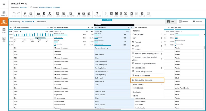
After you create the project, DataBrew provides three different views of the dataset:
- Grid view – Presents the 15 columns and first 1,000 rows sampled from the dataset and the distribution of data across each column
- Schema view – In addition to information in the grid view, presents information about the data types (such as double, integer, or string) and the data quality that indicates the presence of missing or invalid values
- Data profile view – Supported by a data profile job, generates summary statistics such as quartiles, standard deviation, variance, most frequently occurring values, and the correlation between columns
The following screenshot shows our view of the dataset.

Each view presents a unique piece of information that helps us gain a better understanding of the dataset. For instance, in the grid view, we can observe the distribution of data across the 15 columns and spot erroneous data points, such as those with ? in the workclass, occupation, or native-country columns.
In the schema view, we can observe six columns with continuous data, nine columns with categorical or binary data, and no missing or invalid observations in the sample of our dataset. The columns with continuous data also contain the corresponding minimum, maximum, mean, median, and mode values represented as a box plot.
In the data profile view, after running a data profile job, we can observe the summary statistics from the first 20,000 rows, such as the five-number summary, measures of central tendency, variance, skewness, kurtosis, correlations, and the most frequently occurring values in each column. For instance, we can combine the information from the grid view and the data profile view to replace erroneous data points such as ? by the most frequently occurring value in that column as a form of data cleaning. To run a data profile job on more than 20,000 rows, request for a limit increase at [email protected]
As part of the EDA phase, we can look at the distribution of data in the target column, which represents whether a person’s income is above $50,000 per year. The ratio of people whose income is greater than $50,000 per year to those whose income is less than or equal to $50,000 per year is 1:3, indicating that the distribution of the target classes is not imbalanced.
Building a set of data transformation steps and publishing a recipe
Now that we have an intuitive understanding of the dataset, let’s build out the data transformation steps. Based on our EDA, we replace the ? observation with the most frequently occurring value in each column.
- Choose the Replace value or pattern transformation.
- Replace ? with Private in the
workclasscolumn. - Replace ? with United-States in the
native-countrycolumn.

The occupation column also contains observations with ?, but the data points are spread across categories without a clear frequently occurring category. Therefore, we can categorically encode the observations in the occupation column, including those with ? observation, thereby treating ? as a separate category. The occupation column in the adult.data training dataset contains 15 categories, of which Protective-serv, Priv-house-serv, and Armed-Forces occur infrequently. To avoid excessive granularity in ML modeling, we can group these three categories into a single category named Other.
During ML model evaluation and prediction, we can also map categories that the model hasn’t encountered during model training to the Other category.
With that as the background, let’s apply the categorical mapping transformation to only the top 12 distinct values.
- Select Map top 12 values.
- Select Map values to numeric values.
This selects the top 12 categories and combines the other categories into a single category named Other. We now have a new column named occupation_mapped.
- Delete the
occupationcolumn to avoid redundancy. - Similarly, apply the categorical mapping transformation to the top five values in the
workclasscolumn and the top one value in thenative-countryRemember to select Map values to numeric values.
This groups the remaining categories into a single category named Other.
- Delete the columns
workclassandnative-country.
The other four columns with categorical data—marital-status, relationship, race, and sex—have few categories with most of them occurring frequently. Let’s apply the categorical mapping transformation to these columns as well.
- Apply categorical mapping, with the following differences:
- Select Map all values.
- Select Map values to numeric values.
- Delete the original columns to avoid redundancy.
- Delete the
fnlwgtcolumn, because it represents the sampling weight and isn’t related to the target - Delete the
educationcolumn, because it has already been categorically mapped toeducation-num. - Map the
targetcolumn to numeric values, where income less than or equal to $50,000 per year is mapped to class 0 and income greater than $50,000 per year is mapped to class 1. - Rename the destination column to
labelin order to align with our downstream PySpark model training code.

- Delete the original
targetcolumn.
The data preparation phase is now complete, and the set of 20 transformations that consist of data cleaning and categorical mapping is combined into a recipe.

Because the data preparation and ML model training phases are highly iterative, we can save the set of data transformation steps applied by publishing the recipe. This provides version control, and allows us to maintain the data transformation steps and experiment with multiple versions of the recipe in order to determine the version with the best ML model performance. For more information about DataBrew recipes, see Creating and using AWS Glue DataBrew recipes.
Creating and running a DataBrew recipe job
The exploratory data analysis phase helped us gain an intuitive understanding of the dataset, from which we built a recipe to prepare and transform our data for ML modeling. We have been working with a random sample of 1,000 rows from the adult.data training dataset, and we need to apply the same set of data transformation steps to the over 32,000 rows in the adult.data dataset. A DataBrew recipe job provides the ability to scale the transformation steps from a sample of data to the entire dataset. To create our recipe job, complete the following steps:
- On the DataBrew console, choose Jobs.
- Choose Create recipe job.
- For Job name, enter a name.
- Create a new folder in Amazon S3 (
s3://<YOUR-S3-BUCKET-NAME>/transformed-data/) for the recipe job to save the transformed dataset.

The recipe job should take under 2 minutes to complete.
Training an ML model on the transformed dataset using PySpark
With the data transformation job complete, we can use the transformed dataset to train a binary classification model to predict whether a person’s income is above $50,000 per year.
- Create an Amazon EMR notebook.
- When the notebook’s status is Ready, open the notebook in a JupyterLab or Jupyter Notebook environment.
- Choose the PySpark kernel.
For this post, we use Spark version 2.4.6.
- Load the transformed dataset into a PySpark DataFrame within the notebook:
- Inspect the schema of the transformed dataset:
Of the 13 columns in the dataset, we use the first 12 columns as features for the model and the label column as the final target value for prediction.
- Use the
VectorAssemblermethod within PySpark to combine the 12 columns into a single feature vector column, which makes it convenient to train the ML model: - To estimate the model performance on the unseen test dataset (test) split the transformed train dataset (train_dataset_pipline) into 70% for model training and 30% for model validation:
- Train a Random Forest classifier on the training dataset
df_trainand evaluate its performance on the validation datasetdf_valusing the area under the ROC curve (AUC), which is a measure of model performance for binary classifiers at different classification thresholds:
A validation AUC of 0.89 indicates strong model performance for the classifier. Because the data transformation and model training phases are highly iterative in nature, in order to improve the model performance, we can experiment with different data transformation steps, additional features, and other classification models. After we achieve a satisfactory model performance, we can evaluate the model predictions on the unseen test dataset, adult.test.
Evaluating the ML model on the test dataset
In the data transformation and ML model training sections, we have developed a reusable pipeline that we can use to evaluate the model predictions on the unseen test dataset.
- Create a new DataBrew project and load the raw test dataset (
adult.test.csv) from Amazon S3, as we did in the data preparation section. - Import the recipe we created earlier with the 20 data transformation steps to apply them on the
adult.testdataset.


We can observe that all the columns have been transformed successfully, apart from the label column, which contains null values. This is because the adult.test dataset contains messy data in the target column, namely an extra punctuation mark at the end of the classes <=50k and >50k. To correct this, we can remove the last step of the recipe.
- Delete the column
target. - Edit the prior step in creating a categorical map to account for the extra punctuation mark.
- Delete the original target column to avoid redundancy.
- Create and run the recipe job to transform and store the over 16,000 rows in the
adult.testdataset unders3://<YOUR-S3-BUCKET-NAME>/transformed-data/.
This job should take approximately 1 minute to complete.
When the train and test datasets don’t have any variation in the types of categories, we can create and run a recipe job directly from the DataBrew console, without having to create a separate project.
- When the data transformation job on the
adult.testdataset is complete, load the transformed dataset into a PySpark dataframe to evaluate the performance of the binary classification model:
The transformed test dataset has 16281 rows and 13 columns
The model performance with an AUC of 0.89 on the unseen test dataset is about the same as the model performance on the validation set, which demonstrates strong model performance on the unseen test dataset as well.
Summary
In this post, we showed you how to use DataBrew and Amazon EMR to streamline and speed up the data preparation and feature engineering stages of the ML lifecycle. We explored a binary classification problem, but the wide selection of DataBrew pre-built transformations and PySpark ML libraries make this approach extendable to numerous ML use cases.
Get started today! Explore your use case with the services mentioned in this post and many others on the AWS Management Console
About the Authors
 Kartik Kannapur is a Data Scientist with AWS Professional Services. He holds a Master’s degree in Applied Mathematics and Statistics from Stony Brook University and focuses on using machine learning to solve customer business problems.
 Prithiviraj Jothikumar, PhD, is a Data Scientist with AWS Professional Services, where he helps customers build solutions using machine learning. He enjoys watching movies and sports and spending time to meditate.
 Bala Krishnamoorthy is a Data Scientist with AWS Professional Services, where he helps customers solve problems and run machine learning workloads on AWS. He has worked with customers across diverse industries, including software, finance, and healthcare. In his free time, he enjoys spending time outdoors, running with his dog, beating his family and friends at board games and keeping up with the stock market.