Post Syndicated from Melody Yang original https://aws.amazon.com/blogs/big-data/rocksdb-101-optimizing-stateful-streaming-in-apache-spark-with-amazon-emr-and-aws-glue/
Real-time streaming data processing is a strategic imperative that directly impacts business competitiveness. Organizations face mounting pressure to process massive data streams instantaneously—from detecting fraudulent transactions and delivering personalized customer experiences to optimizing complex supply chains and responding to market dynamics milliseconds ahead of competitors.
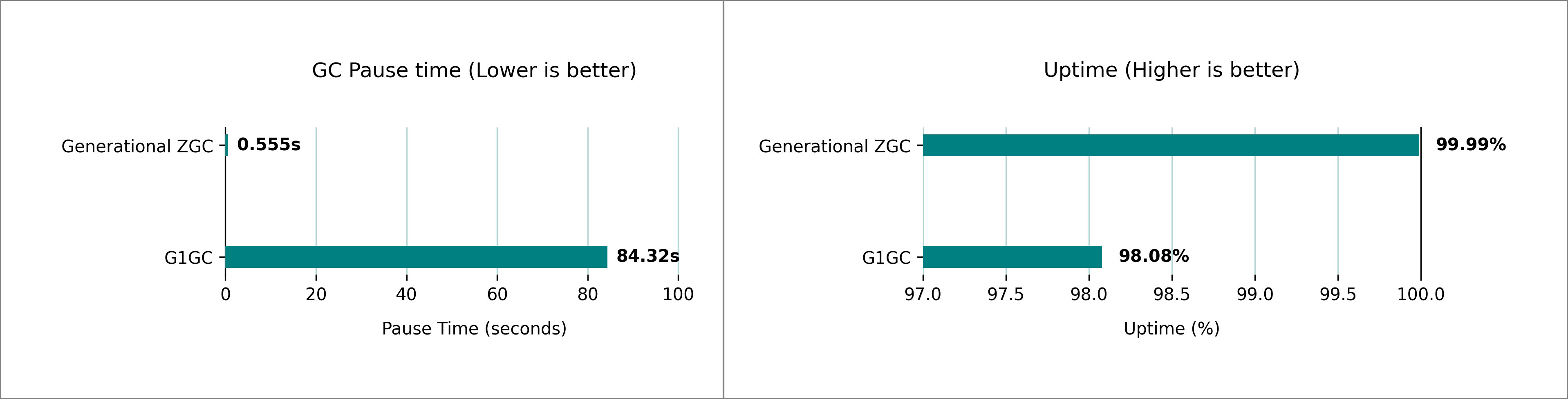
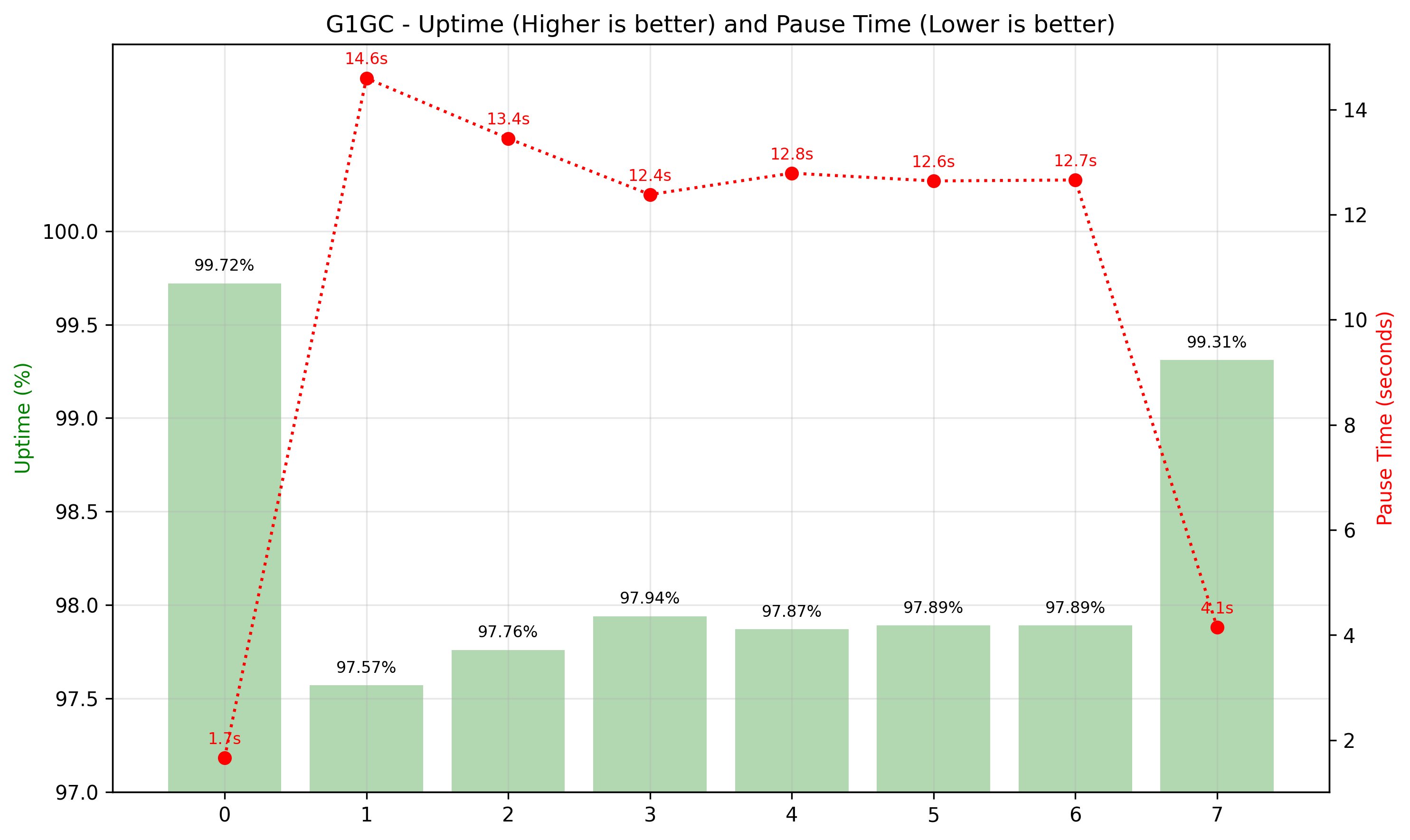
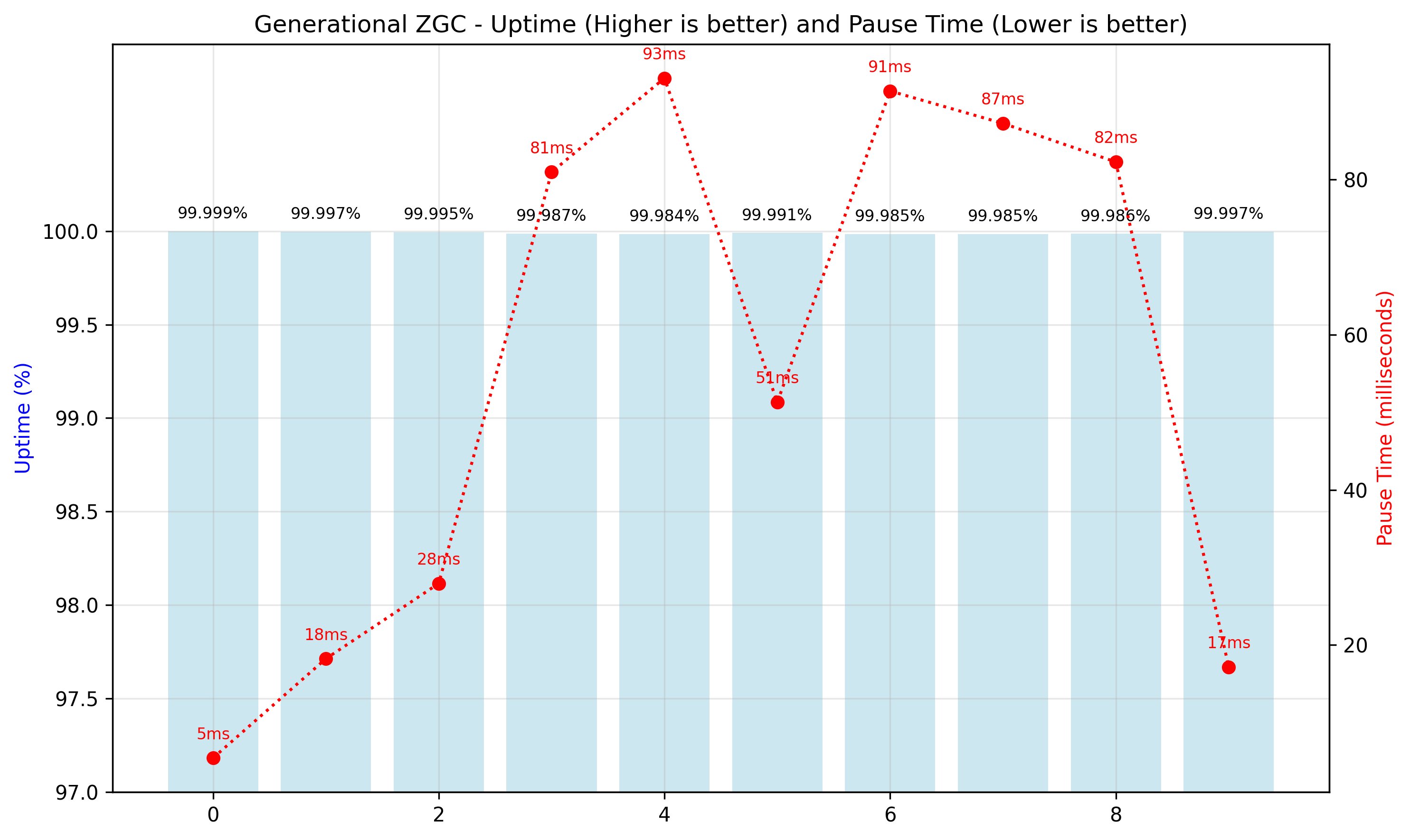
Apache Spark Structured Streaming addresses these critical business challenges through its stateful processing capabilities, enabling applications to maintain and update intermediate results across multiple data streams or time windows. RocksDB was introduced in Apache Spark 3.2, offering a more efficient alternative to the default HDFS-based in-memory store. RocksDB excels in stateful streaming in scenarios that require handling large quantities of state data. It delivers optimal performance benefits, particularly in reducing Java virtual machine (JVM) memory pressure and garbage collection (GC) overhead.
This post explores RocksDB’s key features and demonstrates its implementation using Spark on Amazon EMR and AWS Glue, providing you with the knowledge you need to scale your real-time data processing capabilities.
RocksDB state store overview
Spark Structured Streaming processes fall into two categories:
- Stateful: Requires tracking intermediate results across micro-batches (for example, when running aggregations and de-duplication).
- Stateless: Processes each batch independently.
A state store is required by stateful applications that track intermediate query results. This is essential for computations that depend on continuous events and change results based on each batch of input, or on aggregate data over time, including late arriving data. By default, Spark offers a state store that keeps states in JVM memory, which is performant and sufficient for most general streaming cases. However, if you have a large number of stateful operations in a streaming application—such as, streaming aggregation, streaming dropDuplicates, stream-stream joins, and so on—the default in-memory state store might face out-of-memory (OOM) issues because of a large JVM memory footprint or frequent GC pauses, resulting in degraded performance.
Advantages of RocksDB over in-memory state store
RocksDB addresses the challenges of an in-memory state store through off-heap memory management and efficient checkpointing.
- Off-heap memory management: RocksDB stores state data in OS-managed off-heap memory, reducing GC pressure. While off-heap memory still consumes machine memory, it doesn’t occupy space in the JVM. Instead, its core memory structures, such as block cache or memTables, allocate directly from the operating system, bypassing the JVM heap. This approach makes RocksDB an optimal choice for memory-intensive applications.
- Efficient checkpointing: RocksDB automatically saves state changes to checkpoint locations, such as Amazon Simple Storage Service (Amazon S3) paths or local directories, helping to ensure full fault tolerance. When interacting with S3, RocksDB is designed to improve checkpointing efficiency; it does this through incremental updates and compaction to reduce the amount of data transferred to S3 during checkpoints, and by persisting fewer large state files compared to the many small files of the default state store, reducing S3 API calls and latency.
Implementation considerations
RocksDB operates as a native C++ library embedded within the Spark executor, using off-heap memory. While it doesn’t fall under JVM GC control, it still affects overall executor memory usage from the YARN or OS perspective. RocksDB’s off-heap memory usage might exceed YARN container limits without triggering container termination, potentially leading to OOM issues. You should consider the following approaches to manage Spark’s memory:
Adjust the Spark executor memory size
Increase spark.executor.memoryOverheadorspark.executor.memoryOverheadFactor to leave more room for off-heap usage. The following example sets half (4 GB) of spark.executor.memory (8 GB) as the memory overhead size.
# Total executor memory = 8GB (heap) + 4GB (overhead) = 12GB
spark-submit \
. . . . . . . .
--conf spark.executor.memory=8g \         # JVM Heap
--conf spark.executor.memoryOverhead=4g \ # Off-heap allocation (RocksDB + other native)
. . . . . . . .
For Amazon EMR on Amazon Elastic Compute Cloud (Amazon EC2), enabling YARN memory control with the following strict container memory enforcement through polling method preempts containers to avoid node-wide OOM failures:
yarn.nodemanager.resource.memory.enforced = false
yarn.nodemanager.elastic-memory-control.enabled = false
yarn.nodemanager.pmem-check-enabled = true
or
yarn.nodemanager.vmem-check-enabled = true
Off-heap memory control
Use RocksDB-specific settings to configure memory usage. More details can be found in the Best practices and considerations section.
Get started with RocksDB on Amazon EMR and AWS Glue
To turn on the state store RocksDB in Spark, configure your application with the following setting:
spark.sql.streaming.stateStore.providerClass=org.apache.spark.sql.execution.streaming.state.RocksDBStateStoreProvider
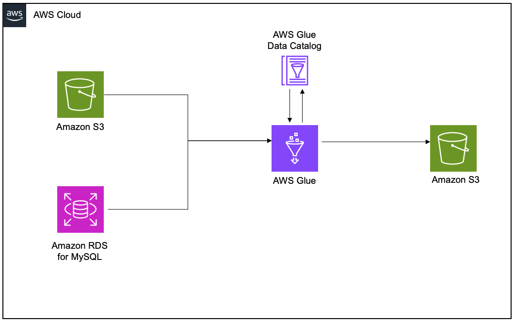
In the following sections, we explore creating a sample Spark Structured Streaming job with RocksDB enabled running on Amazon EMR and AWS Glue respectively.
RocksDB on Amazon EMR
Amazon EMR versions 6.6.0 and later support RocksDB, including Amazon EMR on EC2, Amazon EMR serverless and Amazon EMR on Amazon Elastic Kubernetes Service (Amazon EKS). In this case, we use Amazon EMR on EC2 as an example.
Use the following steps to run a sample streaming job with RocksDB enabled.
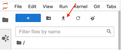
- Upload the following sample script to
s3://<YOUR_S3_BUCKET>/script/sample_script.py
from pyspark.sql import SparkSession
from pyspark.sql.functions import explode, split, col, expr
import random

# List of words
words = ["apple", "banana", "orange", "grape", "melon",
         "peach", "berry", "mango", "kiwi", "lemon"]

# Create random strings from words
def generate_random_string():
    return " ".join(random.choices(words, k=5))


# Create Spark Session
spark = SparkSession \
    .builder \
    .appName("StreamingWordCount") \
    .config("spark.sql.streaming.stateStore.providerClass","org.apache.spark.sql.execution.streaming.state.RocksDBStateStoreProvider") \
    .getOrCreate()


# Register UDF
spark.udf.register("random_string", generate_random_string)

# Create streaming data
raw_stream = spark.readStream \
    .format("rate") \
    .option("rowsPerSecond", 1) \
    .load() \
    .withColumn("words", expr("random_string()"))

# Execute word counts
wordCounts = raw_stream.select(explode(split(raw_stream.words, " ")).alias("word")).groupby("word").count()

# Output the results
query = wordCounts \
    .writeStream \
    .outputMode("complete") \
    .format("console") \
    .start()

query.awaitTermination()
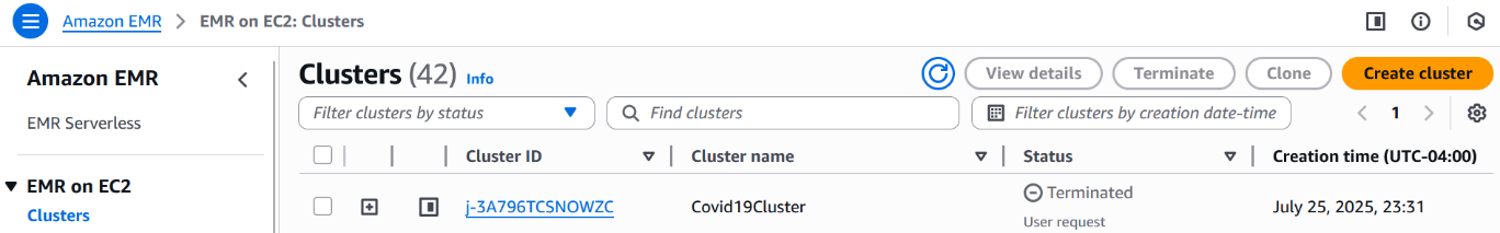
- On the AWS Management Console for Amazon EMR, choose Create Cluster
- For Name and applications – required, select the latest Amazon EMR release.
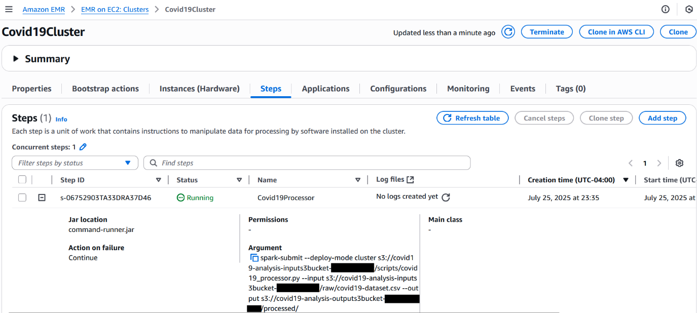
- For Steps, choose Add. For Type, select Spark application.
- For Name, enter
GettingStartedWithRocksDB and s3://<YOUR_S3_BUCKET>/script/sample_script.py as the Application location.
- Choose Save step.
- For other settings, choose the appropriate settings based on your use case.
- Choose Create cluster to start the streaming application via Amazon EMR step.
RocksDB on AWS Glue
AWS Glue 4.0 and later versions support RocksDB. Use the following steps to run the sample job with RocksDB enabled on AWS Glue.
- On the AWS Glue console, in the navigation pane, choose ETL jobs.
- Choose Script editor and Create script.
- For the job name, enter
GettingStartedWithRocksDB.
- Copy the script from the previous example and paste it on the Script tab.
- On Job details tab, for Type, select Spark Streaming.
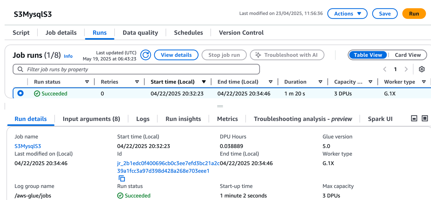
- Choose Save, and then choose Run to start the streaming job on AWS Glue.
Walkthrough details
Let’s dive deep into the script to understand how to run a simple stateful Spark application with RocksDB using the following example pySpark code.
- First, set up RocksDB as your state store by configuring the provider class:
spark = SparkSession \
    .builder \
    .appName("StreamingWordCount") \
    .config("spark.sql.streaming.stateStore.providerClass","org.apache.spark.sql.execution.streaming.state.RocksDBStateStoreProvider") \
    .getOrCreate()
- To simulate streaming data, create a data stream using the
rate source type. It generates one record per second, containing five random fruit names from a pre-defined list.
# List of words
words = ["apple", "banana", "orange", "grape", "melon",
         "peach", "berry", "mango", "kiwi", "lemon"]

# Create random strings from words
def generate_random_string():
    return " ".join(random.choices(words, k=5))
# Register UDF
spark.udf.register("random_string", generate_random_string)

# Create streaming data
raw_stream = spark.readStream \
    .format("rate") \
    .option("rowsPerSecond", 1) \
    .load() \
    .withColumn("words", expr("random_string()"))
- Create a word counting operation on the incoming stream. This is a stateful operation because it maintains running counts between processing intervals, that is, previous counts must be stored to calculate the next new totals.
# Split raw_stream into words and counts them
wordCounts = raw_stream.select(explode(split(raw_stream.words, " ")).alias("word")).groupby("word").count()
- Finally, output the word count totals to the console:
# Output the results
query = wordCounts \
    .writeStream \
    .outputMode("complete") \
    .format("console") \
    .start()
Input data
In the same sample code, test data (raw_stream) is generated at a rate of one-row-per-second, as shown in the following example:
+-----------------------+-----+--------------------------------+
|timestamp              |value|words                           |
+-----------------------+-----+--------------------------------+
|2025-04-18 07:05:57.204|125  |berry peach orange banana banana|
+-----------------------+-----+--------------------------------+
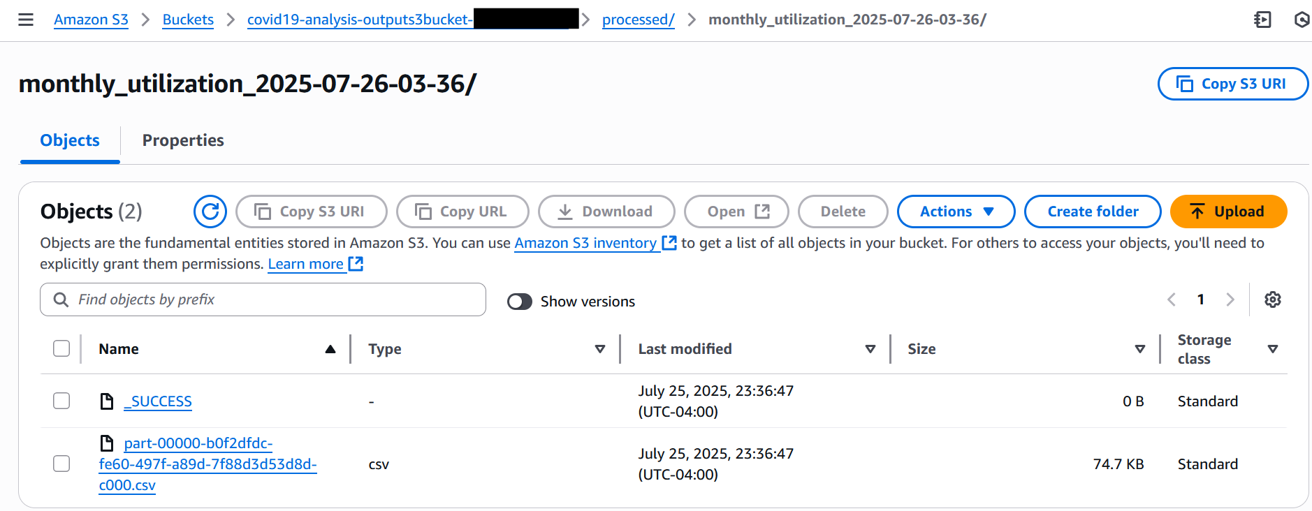
Output result
The streaming job produces the following results in the output logs. It demonstrates how Spark Structured Streaming maintains and updates the state across multiple micro-batches:
- Batch 0: Starts with an empty state
- Batch 1: Processes multiple input records, resulting in initial counts for every one of the 10 fruits (for example, banana appears 8 times)
- Batch 2: Running totals based on new occurrences from the next set of records are added to the counts (for example, banana increases from 8 to 15, indicating 7 new occurrences).
-------------------------------------------
Batch: 0
-------------------------------------------
+----+-----+
|word|count|
+----+-----+
+----+-----+

-------------------------------------------
Batch: 1
-------------------------------------------
+------+-----+
|  word|count|
+------+-----+
|banana|    8|
|orange|    4|
| apple|    3|
| berry|    5|
| lemon|    7|
|  kiwi|    6|
| melon|    8|
| peach|    8|
| mango|    7|
| grape|    9|
+------+-----+

-------------------------------------------
Batch: 2
-------------------------------------------
+------+-----+
|  word|count|
+------+-----+
|banana|   15|
|orange|    8|
| apple|    7|
| berry|   11|
| lemon|   12|
|  kiwi|   11|
| melon|   16|
| peach|   15|
| mango|   12|
| grape|   13|
+------+-----+
State store logs
RocksDB generates detailed logs during the job run, like the following:
INFO    2025-04-18T07:52:28,378 83933   org.apache.spark.sql.execution.streaming.MicroBatchExecution    [stream execution thread for [id = xxxxxxxx-xxxx-xxxx-xxxx-xxxxxxxxxxxx, runId = xxxxxxxx-xxxx-xxxx-xxxx-xxxxxxxxxxxx]] 60  Streaming query made progress: {
  "id": "xxxxxxxx-xxxx-xxxx-xxxx-xxxxxxxxxxxx",
  "runId": "xxxxxxxx-xxxx-xxxx-xxxx-xxxxxxxxxxxx",
  "name": null,
  "timestamp": "2025-04-18T07:52:27.642Z",
  "batchId": 39,
  "numInputRows": 1,
  "inputRowsPerSecond": 100.0,
  "processedRowsPerSecond": 1.3623978201634879,
  "durationMs": {
    "addBatch": 648,
    "commitOffsets": 39,
    "getBatch": 0,
    "latestOffset": 0,
    "queryPlanning": 10,
    "triggerExecution": 734,
    "walCommit": 35
  },
  "stateOperators": [
    {
      "operatorName": "stateStoreSave",
      "numRowsTotal": 10,
      "numRowsUpdated": 4,
      "allUpdatesTimeMs": 18,
      "numRowsRemoved": 0,
      "allRemovalsTimeMs": 0,
      "commitTimeMs": 3629,
      "memoryUsedBytes": 174179,
      "numRowsDroppedByWatermark": 0,
      "numShufflePartitions": 36,
      "numStateStoreInstances": 36,
      "customMetrics": {
        "rocksdbBytesCopied": 5009,
        "rocksdbCommitCheckpointLatency": 533,
        "rocksdbCommitCompactLatency": 0,
        "rocksdbCommitFileSyncLatencyMs": 2991,
        "rocksdbCommitFlushLatency": 44,
        "rocksdbCommitPauseLatency": 0,
        "rocksdbCommitWriteBatchLatency": 0,
        "rocksdbFilesCopied": 4,
        "rocksdbFilesReused": 24,
        "rocksdbGetCount": 8,
        "rocksdbGetLatency": 0,
        "rocksdbPinnedBlocksMemoryUsage": 3168,
        "rocksdbPutCount": 4,
        "rocksdbPutLatency": 0,
        "rocksdbReadBlockCacheHitCount": 8,
        "rocksdbReadBlockCacheMissCount": 0,
        "rocksdbSstFileSize": 35035,
        "rocksdbTotalBytesRead": 136,
        "rocksdbTotalBytesReadByCompaction": 0,
        "rocksdbTotalBytesReadThroughIterator": 0,
        "rocksdbTotalBytesWritten": 228,
        "rocksdbTotalBytesWrittenByCompaction": 0,
        "rocksdbTotalBytesWrittenByFlush": 5653,
        "rocksdbTotalCompactionLatencyMs": 0,
        "rocksdbWriterStallLatencyMs": 0,
        "rocksdbZipFileBytesUncompressed": 266452
      }
    }
  ],
  "sources": [
    {
      "description": "RateStreamV2[rowsPerSecond=1, rampUpTimeSeconds=0, numPartitions=default",
      "startOffset": 63,
      "endOffset": 64,
      "latestOffset": 64,
      "numInputRows": 1,
      "inputRowsPerSecond": 100.0,
      "processedRowsPerSecond": 1.3623978201634879
    }
  ],
  "sink": {
    "description": "org.apache.spark.sql.execution.streaming.ConsoleTable$@2cf39784",
    "numOutputRows": 10
  }
}
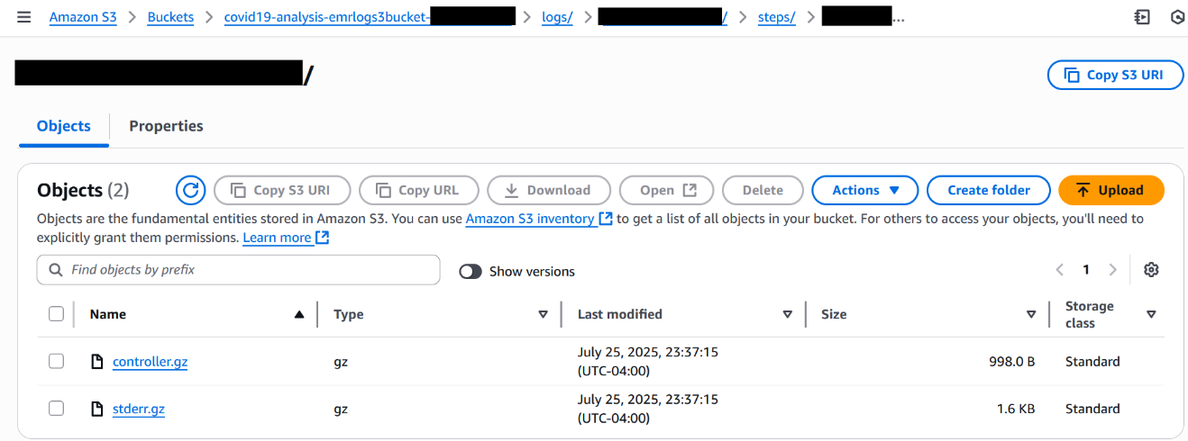
In Amazon EMR on EC2, these logs are available on the node where the YARN ApplicationMaster container is running. They can be found at/var/log/hadoop-yarn/containers/<Application ID>/<container_id>/stderr.
As for AWS Glue, you can find the RocksDB metrics in Amazon CloudWatch, under the log group /aws-glue/jobs/error.
RocksDB metrics
The metrics from the preceding logs provide insights on RocksDB status. The followings are some example metrics you might find useful when investigating streaming job issues:
rocksdbCommitCheckpointLatency: Time spent writing checkpoints to local storagerocksdbCommitCompactLatency: Duration of checkpoint compaction operations during checkpoint commitsrocksdbSstFileSize: Current size of SST files in RocksDB.
Deep dive into RocksDB key concepts
To better understand the state metrics shown in the logs, we deep dive into RocksDB’s key concepts: MemTable, sorted string table (SST) file, and checkpoints. Additionally, we provide some tips for best practices and fine-tuning.
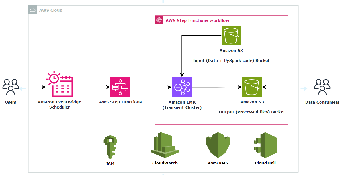
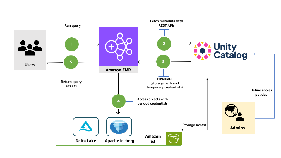
High level architecture

RocksDB is a local, non-distributed persistent key-value store embedded in Spark executors. It enables scalable state management for streaming workloads, backed by Spark’s checkpointing for fault tolerance. As shown in the preceding figure, RocksDB stores data in memory and also on disk. RocksDB’s ability to spill data over to disk is what allows Spark Structured Streaming to handle state data that exceeds the available memory.
Memory:
- Write buffers (MemTables): Designated memory to buffer writes before flushing onto disk
- Block cache (read buffer): Reduces query time by caching results from disk
Disk:
- SST files: Sorted String Table saved as SST file format for fast access
MemTable: Stored off-heap

MemTable, shown in the preceding figure, is an in-memory store where data is first written off-heap, before being flushed to disk as an SST file. RocksDB caches the latest two batches of data (hot data) in MemTable to reduce streaming process latency. By default, RocksDB only has two MemTables—one is active and the other is read-only. If you have sufficient memory, the configuration spark.sql.streaming.stateStore.rocksdb.maxWriteBufferNumber can be increased to have more than two MemTables. Among these MemTables, there is always one active table, and the rest are read-only MemTables used as write buffers.
SST files: Stored on Spark executor’s local disk
SST files are block-based tables stored on the Spark executor’s local disk. When the in-memory state data can no longer fit into a MemTable (defined by a Spark configuration writeBufferSizeMB), the active table is marked as immutable, saving it as the SST file format, which switches it to a read-only MemTable while asynchronously flushing it to local disks. While flushing, the immutable MemTable can still be read, so that the most recent state data is available with minimal read latency.

Reading from RocksDB follows the sequence demonstrated by the preceding diagram:
- Read from the active MemTable.
- If not found, iterate through read-only MemTables in the order of newest to oldest.
- If not found, read from BlockCache (read buffer).
- If misses, load index (one index per SST) from disk into BlockCache. Look up key from index and if hits, load data block onto BlockCache and return result.
SST files are stored on executors’ local directories under the path of spark.local.dir (default: /tmp) or yarn.nodemanager.local-dirs:
- Amazon EMR on EC2 –
${yarn.nodemanager.local-dirs}/usercache/hadoop/appcache/<yarn_app_id>/<spark_app_id>/
- Amazon EMR Serverless, Amazon EMR on EKS, AWS Glue –
${spark.local.dir}/<spark_app_id>/
Additionally, by using application logs, you can track the MemTable flush and SST file upload status under the file path:
- Amazon EMR on EC2 –
/var/log/hadoop-yarn/containers/<application_id>/<container_id>/stderr
- Amazon EMR on EKS –
/var/log/spark/user/<spark_app_name>-<spark_executor_ID>/stderr
The following is an example command to check the SST file status in an executor log from Amazon EMR on EKS:
cat /var/log/spark/user/<spark_app_name>-<spark_executor_ID>/stderr/current | grep old
or
kubectl logs <spark_executor_pod_name> --namespace emr -c spark-kubernetes-executor | grep old
The following screenshot is an example of the output of either command.

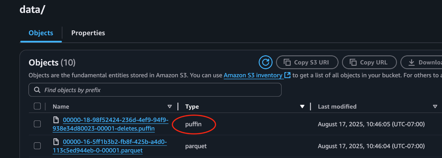
You can use the following examples to check if the MemTable records were deleted and flushed out to SST:
cat /var/log/spark/user/<spark_app_name>-<spark_executor_ID>/stderr/current | grep deletes
or
kubectl logs <spark_executor_pod_name> --namespace emr -c spark-kubernetes-executor | grep deletes
The following screenshot is an example of the output of either command.

Checkpoints: Stored on the executor’s local disk or in an S3 bucket
To handle fault tolerance and fail over from the last committed point, RocksDB supports checkpoints. The checkpoint files are usually stored on the executor’s disk or in an S3 bucket, including snapshot and delta or changelog data files.
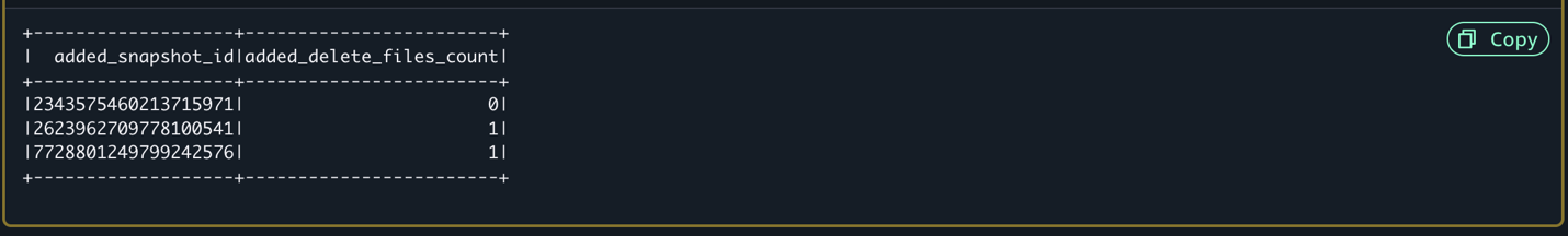
Starting with Amazon EMR 7.0 and AWS Glue5.0, RocksDB state store provides a new feature called changelog checkpointing to enhance checkpoint performance. when the changelog is enabled (disabled by default) using the setting spark.sql.streaming.stateStore.rocksdb.changelogCheckpointing.enabled, RocksDB writes smaller change logs to the storage location (the local disk by default) instead of frequently persisting large snapshot data. Note that snapshots are still created but less frequently, as shown in the following screenshot.

Here’s an example of a checkpoint location path when overridden to an S3 bucket: s3://<S3BUCKET>/<checkpointDir>/state/0/spark_parition_ID/state_version_ID.zip
Best practices and considerations
This section outlines key strategies for fine-tuning RocksDB performance and avoiding common pitfalls.
1. Memory management for RocksDB
To prevent OOM errors on Spark executors, you can configure RocksDB’s memory usage at either the node level or instance level:
- Node level (recommended): Enforce a global off-heap memory limit per executor. In this context, each executor is treated as a RocksDB node. If an executor processes N partitions of a stateful operator, it will have N number of RocksDB instances on a single executor.
- Instance-level: Fine-tune individual RocksDB instances.
Node-level memory control per executor
Starting with Amazon EMR 7.0 and AWS Glue 5.0 (Spark 3.5), a critical Spark configuration, boundedMemoryUsage, was introduced (through SPARK-43311) to enforce a global memory cap at a single executor level that is shared by multiple RocksDB instances. This prevents RocksDB from consuming unbounded off-heap memory, which could lead to OOM errors or executor termination by resource managers such as YARN or Kubernetes.
The following example shows the node-level configuration:
 # Bound total memory usage per executor
 "spark.sql.streaming.stateStore.rocksdb.boundedMemoryUsage": "true"
 # Set a static total memory size per executor
 "spark.sql.streaming.stateStore.rocksdb.maxMemoryUsageMB": "500"
 # For read-heavy workloads, split memory allocation between write buffers (30%) and block cache (70%)
 "spark.sql.streaming.stateStore.rocksdb.writeBufferCacheRatio": "0.3"
A single RocksDB instance level control
For granular memory management, you can configure individual RocksDB instances using the following settings:
# Control MemTable (write buffer) size and count
"spark.sql.streaming.stateStore.rocksdb.writeBufferSizeMB": "64"
"spark.sql.streaming.stateStore.rocksdb.maxWriteBufferNumber": "4"
- writeBufferSizeMB (default: 64, suggested: 64 – 128): Controls the maximum size of a single MemTable in RocksDB, affecting memory usage and write throughput. This setting is available in Spark3.5 – [SPARK-42819] and later. It determines the size of the memory buffer before state data is flushed to disk. Larger buffer sizes can improve write performance by reducing SST flush frequency but will increase the executor’s memory usage. Adjusting this parameter is crucial for optimizing memory usage and write throughput.
- maxWriteBufferNumber (default: 2, suggested: 3 – 4): Sets the total number of active and immutable MemTables.
For read-heavy workloads, prioritize the following block cache tuning over write buffers to reduce disk I/O. You can configure SST block size and caching as follows:
"spark.sql.streaming.stateStore.rocksdb.blockSizeKB": "64"
"spark.sql.streaming.stateStore.rocksdb.blockCacheSizeMB": "128"
- blockSizeKB (default: 4, suggested: 64–128): When an active MemTable is full, it becomes a read-only memTable. From there, new writes continue to accumulate in a new table. The read-only MemTable is flushed into SST files on the disk. The data in SST files is approximately chunked into fixed-sized blocks (default is 4 KB). Each block, in turn, keeps multiple data entries. When writing data to SST files, you can compress or encode data efficiently within a block, which often results in a smaller data size compared with its raw format.
For workloads with a small state size (such as less than 10 GB), the default block size is usually sufficient. For a large state (such as more than 50 GB), increasing the block size can improve compression efficiency and sequential read performance but increase CPU overhead.
- blockCacheSizeMB (default: 8, suggested: 64–512, large state: more than
1024): When retrieving data from SST files, RocksDB provides a cache layer (block cache) to improve the read performance. It first locates the data block where the target record might reside, then caches the block to memory, and finally searches that record within the cached block. To avoid frequent reads of the same block, the block cache can be used to keep the loaded blocks in memory.
2. Clean up state data at checkpoint
To help ensure that your state file sizes and storage costs remain under control when checkpoint performance becomes a concern, use the following Spark configurations to adjust cleanup frequency, retention limits, and checkpoint file types:
# clean up RocksDB state every 30 seconds
"spark.sql.streaming.stateStore.maintenanceInterval":"30s"
# retain only the last 50 state versions
"spark.sql.streaming.minBatchesToRetain":"50"
# use changelog instead of snapshots
"spark.sql.streaming.stateStore.rocksdb.changelogCheckpointing.enabled":"true"
- maintenanceInterval (default: 60 seconds): Retaining a state for a long period of time can help reduce maintenance cost and background IO. However, longer intervals increase file listing time, because state stores often scan every retained file.
- minBatchesToRetain (default: 100, suggested: 10–50): Limits the number of state versions retained at checkpoint locations. Reducing this number results in fewer files being persisted and reduces storage usage.
- changelogCheckpointing (default: false, suggested: true): Traditionally, RocksDB snapshots and uploads incremental SST files to checkpoint. To avoid this cost, changelog checkpointing was introduced in Amazon EMR7.0+ and AWS Glue 5.0, which write only state changes since the last checkpoint.
To track an SST file’s retention status, you can search RocksDBFileManager entries in the executor logs. Consider the following logs in Amazon EMR on EKS as an example. The output (shown in the screenshot) shows that four SST files under version 102 were uploaded to an S3 checkpoint location, and that an old changelog state file with version 97 was cleaned up.
cat /var/log/spark/user/<spark_app_name>-<spark_executor_ID>/stderr/ current | grep RocksDBFileManager
or
kubectl logs <spark_executor_pod_name> -n emr -c spark-kubernetes-executor | grep RocksDBFileManager

3. Optimize local disk usage
RocksDB consumes local disk space when generating SST files at each Spark executor. While disk usage doesn’t scale linearly, RocksDB can accumulate storage over time based on state data size. When running streaming jobs, if local available disk space gets insufficient, No space left on device errors can occur.
To optimize disk usage by RocksDB, adjust the following Spark configurations:
# compact state files during commit (default:false)
"spark.sql.streaming.stateStore.rocksdb.compactOnCommit": "true"
# number of delta SST files before becomes a consolidated snapshot file(default:10)
"spark.sql.streaming.stateStore.minDeltasForSnapshot": "5"
Infrastructure adjustments can further mitigate the disk issue:
For Amazon EMR:
For AWS Glue:
- Use AWS Glue G.2X or larger worker types to avoid the limited disk capacity of G.1X workers.
- Schedule regular maintenance windows at optimal timing to free up disk space based on workload needs.
Conclusion
In this post, we explored RocksDB as the new state store implementation in Apache Spark Structured Streaming, available on Amazon EMR and AWS Glue. RocksDB offers advantages over the default HDFS-backed in-memory state store, particularly for applications dealing with large-scale stateful operations. RocksDB helps prevent JVM memory pressure and garbage collection issues common with the default state store.
The implementation is straightforward, requiring minimal configuration changes, though you should pay careful attention to memory and disk space management for optimal performance. While RocksDB is not guaranteed to reduce job latency, it provides a robust solution for handling large-scale stateful operations in Spark Structured Streaming applications.
We encourage you to evaluate RocksDB for your use cases, particularly if you’re experiencing memory pressure issues with the default state store or need to handle large amounts of state data in your streaming applications.
About the authors
 Melody Yang is a Senior Big Data Solution Architect for Amazon EMR at AWS. She is an experienced analytics leader working with AWS customers to provide best practice guidance and technical advice in order to assist their success in data transformation. Her areas of interests are open-source frameworks and automation, data engineering and DataOps.
Dai Ozaki is a Cloud Support Engineer on the AWS Big Data Support team. He is passionate about helping customers build data lakes using ETL workloads. In his spare time, he enjoys playing table tennis.
Noritaka Sekiyama is a Principal Big Data Architect with Amazon Web Services (AWS) Analytics services. He’s responsible for building software artifacts to help customers. In his spare time, he enjoys cycling on his road bike.
 Amir Shenavandeh is a Sr Analytics Specialist Solutions Architect and Amazon EMR subject matter expert at Amazon Web Services. He helps customers with architectural guidance and optimisation. He leverages his experience to help people bring their ideas to life, focusing on distributed processing and big data architectures.
Xi Yang is a Senior Hadoop System Engineer and Amazon EMR subject matter expert at Amazon Web Services. He is passionate about helping customers resolve challenging issues in the Big Data area.


 Atul Felix Payapilly is a software development engineer for Amazon EMR at Amazon Web Services.
 Akshaya KP is a software development engineer for Amazon EMR at Amazon Web Services.
 Giovanni Matteo is the Senior Manager for the Amazon EMR Spark and Iceberg group.
 Suvojit Dasgupta is a Principal Data Architect at Amazon Web Services. He leads a team of skilled engineers in designing and building scalable data solutions for diverse customers. He specializes in developing and implementing innovative data architectures to address complex business challenges.
 Peter Manastyrny is a Senior Product Manager at AWS Analytics. He leads Amazon EMR on EKS, a product that makes it straightforward and efficient to run open-source data analytics frameworks such as Spark on Amazon EKS.
 Matt Poland is a Senior Cloud Infrastructure Architect at Amazon Web Services. He is passionate about solving complex problems and delivering well-structured solutions for diverse customers. His expertise spans across a range of cloud technologies, providing scalable and reliable infrastructure tailored to each project’s unique challenges.
 Gregory Fina is a Principal Startup Solutions Architect for Generative AI at Amazon Web Services, where he empowers startups to accelerate innovation through cloud adoption. He specializes in application modernization, with a strong focus on serverless architectures, containers, and scalable data storage solutions. He is passionate about using generative AI tools to orchestrate and optimize large-scale Kubernetes deployments, as well as advancing GitOps and DevOps practices for high-velocity teams. Outside of his customer-facing role, Greg actively contributes to open source projects, especially those related to Backstage.


 Gagan Brahmi is a Specialist Senior Solutions Architect at Amazon Web Services (AWS), specializing in Data Analytics and AI/ML solutions. With over 20 years in information technology, he helps customers architect scalable, high-performance analytics platforms using distributed data processing, real-time streaming technologies, and machine learning services on AWS. When not designing cloud solutions, Gagan enjoys exploring new places with his family.
 Arun Shanmugam is a Senior Analytics Solutions Architect at AWS, with a focus on building modern data architecture. He has been successfully delivering scalable data analytics solutions for customers across diverse industries. Outside of work, Arun is an avid outdoor enthusiast who actively engages in CrossFit, road biking, and cricket.
 George Oakes is a Senior Hybrid Solutions Architect at AWS, with a focus on edge, on-premise, and low latency architectures. He has been successfully delivering scalable hybrid AWS solutions for customers across diverse industries. Outside of work, George is an avid outdoor enthusiast who enjoys hiking and visiting parks and UNESCO sites around.


 Venkatavaradhan (Venkat) Viswanathan is a Global Partner Solutions Architect at Amazon Web Services. Venkat is a Technology Strategy Leader in Data, AI, ML, generative AI, and Advanced Analytics. Venkat is a Global SME for Databricks and helps AWS customers design, build, secure, and optimize Databricks workloads on AWS.
 Srividya Parthasarathy is a Senior Big Data Architect on the AWS Lake Formation team. She works with the product team and customers to build robust features and solutions for their analytical data platform. She enjoys building data mesh solutions and sharing them with the community.
 Ramkumar Nottath is a Principal Solutions Architect at AWS focusing on Analytics services. He enjoys working with various customers to help them build scalable, reliable big data and analytics solutions. His interests extend to various technologies such as analytics, data warehousing, streaming, data governance, and machine learning. He loves spending time with his family and friends.
 John Spencer is a Product Manager at Databricks, dedicated to making Unity Catalog work seamlessly with customers’ ecosystems of tools and platforms so they can easily access, govern, and use their data.
 Sreeram Thoom is a Specialist Solutions Architect at Databricks helping customers design secure, scalable applications on the Data Lakehouse.
 Dipankar Kushari is a specialist solutions architect at Databricks helping customer architect and build secured applications on Data Lakehouse.


 Melody Yang is a Senior Big Data Solution Architect for Amazon EMR at AWS. She is an experienced analytics leader working with AWS customers to provide best practice guidance and technical advice in order to assist their success in data transformation. Her areas of interests are open-source frameworks and automation, data engineering and DataOps.
 Dai Ozaki is a Cloud Support Engineer on the AWS Big Data Support team. He is passionate about helping customers build data lakes using ETL workloads. In his spare time, he enjoys playing table tennis.
 Noritaka Sekiyama is a Principal Big Data Architect with Amazon Web Services (AWS) Analytics services. He’s responsible for building software artifacts to help customers. In his spare time, he enjoys cycling on his road bike.
 Xi Yang is a Senior Hadoop System Engineer and Amazon EMR subject matter expert at Amazon Web Services. He is passionate about helping customers resolve challenging issues in the Big Data area.


 Aarthi Srinivasan is a Senior Big Data Architect with Amazon SageMaker Lakehouse. As part of the SageMaker Lakehouse team, she works with AWS customers and partners to architect lake house solutions, enhance product features, and establish best practices for data governance.
 Praveen Kumar is an Analytics Solutions Architect at AWS with expertise in designing, building, and implementing modern data and analytics platforms using cloud-based services. His areas of interest are serverless technology, data governance, and data-driven AI applications.
 Dhananjay Badaya is a Software Developer at AWS, specializing in distributed data processing engines including Apache Spark and Apache Hadoop. As a member of the Amazon EMR team, he focuses on designing and implementing enterprise governance features for EMR Spark.


 Sri Potluri is a Cloud Infrastructure Architect at AWS. He is passionate about solving complex problems and delivering well-structured solutions for diverse customers. His expertise spans across a range of cloud technologies, providing scalable and reliable infrastructures tailored to each project’s unique challenges.
 Suvojit Dasgupta is a Principal Data Architect at AWS. He leads a team of skilled engineers in designing and building scalable data solutions for AWS customers. He specializes in developing and implementing innovative data architectures to address complex business challenges.


 Shubham Purwar is an AWS Analytics Specialist Solution Architect. He helps organizations unlock the full potential of their data by designing and implementing scalable, secure, and high-performance analytics solutions on the AWS platform. With deep expertise in AWS analytics services, he collaborates with customers to uncover their distinct business requirements and create customized solutions that deliver actionable insights and drive business growth. In his free time, Shubham loves to spend time with his family and travel around the world.
 Nitin Kumar is a Cloud Engineer (ETL) at AWS, specialized in AWS Glue. With a decade of experience, he excels in aiding customers with their big data workloads, focusing on data processing and analytics. He is committed to helping customers overcome ETL challenges and develop scalable data processing and analytics pipelines on AWS. In his free time, he likes to watch movies and spend time with his family.
 Prashanthi Chinthala is a Cloud Engineer (DIST) at AWS. She helps customers overcome EMR challenges and develop scalable data processing and analytics pipelines on AWS.