Post Syndicated from Rajiv Gupta original https://aws.amazon.com/blogs/big-data/getting-the-most-out-of-your-analytics-stack-with-amazon-redshift/
Analytics environments today have seen an exponential growth in the volume of data being stored. In addition, analytics use cases have expanded, and data users want access to all their data as soon as possible. The challenge for IT organizations is how to scale your infrastructure, manage performance, and optimize for cost while meeting these growing demands.
As a Sr. Analytics Solutions Architect at AWS, I get to learn firsthand about these challenges and work with our customers to help them design and optimize their architecture. Amazon Redshift is often a key component in that analytics stack. Amazon Redshift has several built-in features to give you out-of-the-box performance, such as automatic workload management, automatic ANALYZE, automatic VACUUM DELETE, and automatic VACUUM SORT. These tuning features enable you to get the performance you need with fewer resources. In addition, Amazon Redshift provides the Amazon Redshift Advisor, which continuously scans your Amazon Redshift cluster and provides recommendations based on best practices. All you need to do is review the recommendations and apply the ones that provide the most benefit.
In this post, we examine a few challenges to your continually evolving analytics environment and how you can configure it to get the most out of your analytics stack by using the new innovations in Amazon Redshift.
Choosing the optimal hardware
The first area to consider is to ensure that you’ve chosen the optimal node type for your workload. Amazon Redshift has three families of node types; RA3, DC2, and DS2. The newest node type, RA3, was built for compute and storage separation so you can cost-effectively scale storage and compute to handle most analytics workloads, and should be chosen for most customers. If you have smaller datasets (< 640 GB of compressed data) or heavier compute needs, you may want to consider the DC2 nodes. Finally, the DS2 node type, while still available, is considered a legacy node type. If you’re using the DS2 node type, you should migrate to RA3 to optimize costs and performance. One of the key benefits of cloud computing is that you’re not tied to one node type. It’s very fast and efficient to migrate between one node type to another using the elastic resize functionality. Because all node types are compatible, no code changes are necessary.
For each node type, there are different sizes to consider. For the RA3 node type, there are the XLPlus, 4XLarge and 16XLarge sizes, for the DC2 node types, the Large and 8XLarge sizes and for for DS2, the XLarge and 8XLarge sizes. The following table summarizes the allocated resources for each instance type as of December 11, 2020.
| Instance type | Disk type | Size | Memory | vCPUs | Maximum Nodes |
| RA3 xlplus | Managed Storage | Scales to 32 TB* | 32 GB | 4 | 16 |
| RA3 4xlarge | Managed Storage | Scales to 64 TB* | 96 GB | 12 | 32 |
| RA3 16xlarge | Managed Storage | Scales to 128 TB* | 384 GB | 48 | 128 |
| DC2 large | SSD | 160 GB | 16 GB | 2 | 32 |
| DC2 8xlarge | SSD | 2.56 TB | 244 GB | 32 | 128 |
| DS2 xlarge | Magnetic | 2 TB | 32 GB | 4 | 32 |
| DS2 8xlarge | Magnetic | 16 TB | 244 GB | 36 | 128 |
When determining the node size and the number of nodes needed in your cluster, consider your processing needs. For the node type you’re using, start with the smallest node size and consider the larger node sizes when you exceed the threshold of number of nodes. For example, for the RA3.XLPlus node type, the maximum number of nodes is 16 nodes. When you exceed this, consider 6 or more of the RA3.4XLarge node. When you exceed 32 nodes of the RA3.4XLarge node type, consider 8 or more of the RA3.16XLarge node. The Amazon Redshift console (see the following screenshot) provides a helpful tool to help you size your cluster taking into consideration parameters such as the amount of storage you need as well as your workload.

Reserving compute power
Building and managing a data warehouse environment is a large cross-functional effort often involving an investment in both time and resources. Amazon Redshift provides deep discounts on the hardware needed to run your data warehouse if you reserve your instances. After you’ve evaluated your workloads and have a configuration you like, purchase Reserved Instances (RIs) for discounts from 20% to 75% when compared to on-demand. You can purchase RIs using a Full Upfront, Partial Upfront, or sometimes a No Upfront payment plan. Reserved Instances are not tied to a particular cluster and are pooled across your account. If your needs expand and you decide to increase your cluster size, simply purchase additional Reserved Instances.
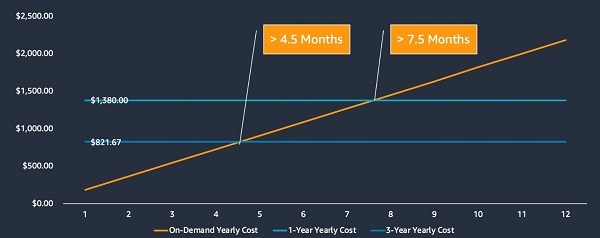
In the following chart, you can compare the yearly on-demand cost of a Redshift cluster to the equivalent cost of a 1-year RI and a 3-year RI (sample charges and discounts are based on 1 node of dc2.large all upfront commitments in the us-east-1 Region as published on November 1st, 2020). If you use your cluster for more than 7.5 months of the year, you save money with the purchase of a 1-year RI. If you use your cluster for more than 4.5 months on-demand, you can save even more money with the purchase of a 3-year RI.
Managing intermittent workloads
If your workload is infrequently accessed, Amazon Redshift allows you to pause and resume your cluster. When your cluster is paused, you’re only charged for backup and storage costs. You can pause and resume your cluster using an API command, the Amazon Redshift console, or through a scheduler. One use case where this feature is useful is if you’re using Amazon Redshift as a compute engine that reads data from the Amazon Simple Storage Service (Amazon S3) data lake and unloads the results back to the data lake. In that use case, you only need the cluster running during the data curation process. Another use case where this feature may be useful is if the cluster only needs to be available when the data pipeline runs and for a reporting platform to refresh its in-memory storage.
When deciding to pause and resume your cluster, keep in mind the cost savings from Reserved Instances. In the following chart, we can compare the daily on-demand cost of an Amazon Redshift cluster to the equivalent cost of a 1-year RI and a 3-year RI when divided by the number of days in the RI (sample charges and discounts are based on 1 node of dc2.large all upfront commitments in the us-east-1 Region as published on November 1st, 2020). If you use your cluster for more than 15 hours in a day, you save money with the purchase of a 1-year RI. If you use your cluster for more than 9 hours in a day, you can save even more money with the purchase of a 3-year RI.

Managing data growth with RA3
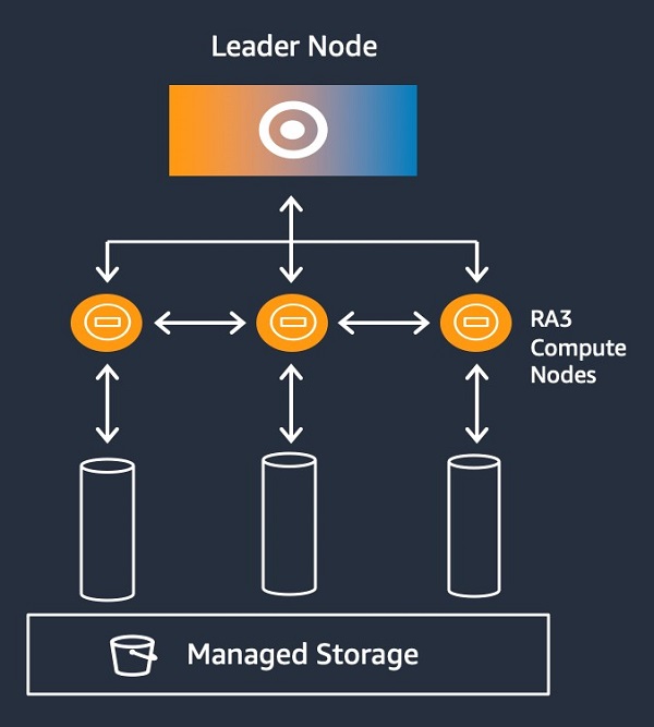
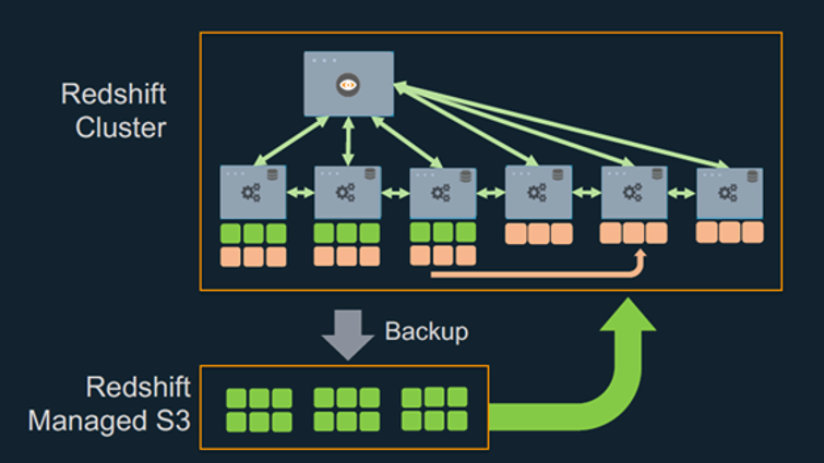
With use cases expanding, there is more and more demand for data within the analytics environment. In many cases, data growth outpaces the compute needs. In traditional MPP systems, to manage data growth, you could add nodes to your cluster, archive old data, or make choices on which data to include. With Amazon Redshift RA3 with managed storage, instead of the primary storage being on your compute nodes, your primary storage is backed by Amazon S3, which allows for much greater storage elasticity. The compute nodes contain a high-performance SSD backed local cache of your data. Amazon Redshift automatically moves hot data to cache so that processing the hottest data is fast and efficient. This removes the need to worry about storage so you can scale your cluster based on your compute needs. Migrating to RA3 is fast and doesn’t require making any configuration changes. You simply resize your cluster and choose the node type and number of nodes for your target configuration. The following diagram illustrates this architecture.
Managing real-time analytics with federated query
We often see the use case of wanting a unified view of your data that is accessible within your analytics environment. That data might be high-volume log or sensor data that is being streamed into the data lake, or operational data that is generated in an OLTP database. With Amazon Redshift, instead of building pipelines to ingest that data into your data warehouse, you can use you can use the federated query feature and Amazon Redshift Spectrum to expose this data as external schemas and tables for direct querying, joining, and processing. Querying data in place reduces both the storage needs and compute needs of your data warehouse. The query engine de-composes the query and determines which parts of the query processing can be run in the source system. When possible, filters and transformations are pushed down to the source. In the case of an OLTP database, any applicable filters are applied to the query in Amazon Aurora PostgreSQL or Amazon RDS for PostgreSQL. In the case of the data lake, the processing occurs in the Amazon Redshift Spectrum compute layer. The following diagram illustrates this architecture.

Managing data growth with compression
When you analyze the steps involved in running a query, I/O operations are usually the most time-consuming step. You can reduce the number of I/O operations and maximize resources in your analytics environment by optimizing storage. Amazon Redshift is a columnar store database and organizes data in 1 MB blocks. The more data that can fit in a 1 MB block, the less I/O operations are needed for reads and writes.
For every column in Amazon Redshift, you can choose the compression encoding algorithm. Because the column compression is so important, Amazon Redshift developed a new encoding algorithm: AZ64. This proprietary algorithm is intended for numeric and data/time data types. Benchmarking AZ64 against other popular algorithms (ZSTD and LZO) showed better performance and sometimes better storage savings. To apply a column encoding, you typically specify the encoding in the CREATE TABLE statement. If you don’t specifically set a column encoding, Amazon Redshift chooses the most optimal based on the data type you specified either at table creation or when it is first loaded. If you have older tables, they may not be taking advantage of the latest encoding algorithms. You can modify the encoding using the ALTER TABLE statement. The following table summarizes your storage savings and performance improvements.

Managing spiky workloads with concurrency scaling
Analytic workloads rarely have even compute requirements 24/7. Instead, spikes appear throughout the day, whether it’s because of an ingestion pipeline or a spike in user activity related to a business event that is out of your control.
When user demand is unpredictable, you can use the concurrency scaling feature to automatically scale your cluster. When the cluster sees a spike in user activity, concurrency scaling detects that spike and automatically routes queries to a new cluster within seconds. Queries run on the concurrent cluster without any change to your application and don’t require data movement. You can configure concurrency scaling to use up to 10 concurrent clusters, but it only uses the clusters it needs for the time it needs them. When your query runs against the concurrent cluster, you only pay for the amount of time the query is run and billed per second. The following diagram illustrates this architecture.

Each cluster earns up to 1 hour of free concurrency scaling credits per day, which is sufficient for 97% of customers. You can also set up costs controls using the usage limits. This feature can alert you or even disable the feature if you exceed a certain amount of usage.
Managing spiky workloads with elastic resize
When the user demand is predictable, you can use the elastic resize feature to easily scale your cluster up and down using an API command, the console, or based on a schedule. For example, if you have an ETL workload every night that requires additional I/O capacity, you can schedule a resize to occur every evening during your ETL workload. During an elastic resize, the endpoint doesn’t change and it happens within minutes. If a session connection is running, it’s paused until the resize completes. You can then scale back down at the end of the ETL workload. The following diagram illustrates this process.
Whether it’s through elastic resize or concurrency scaling, you want to size based on your steady state compute needs, not the peaks, and use features like elastic resize and concurrency scaling.
Providing access to shared data through multiple clusters
You may have multiple groups within your organization who want to access the analytics data. One option is to load all the data into one Amazon Redshift cluster and size the cluster to meet the compute needs of all users. However, that option can be costly. Also, isolating the workloads for some of your groups provides a few benefits. Each organization can be responsible for their own cluster charges and if either group has a tight SLA, they can ensure that the other’s queries don’t cause resource contention. One solution for sharing data and isolating workloads is by using the lake house architecture. When you manage your data in a data lake, you can keep it in open formats that are easily transportable and readable by any number of analytics services. Capabilities such as Amazon Redshift Spectrum, data lake export, and INSERT (external table), enable you to easily read and write data from a shared data lake within Amazon Redshift. Each group can live query the external data and join it to any local data they may have. Each group may even consider pausing and resuming their cluster when it is not in use. The following diagram illustrates this architecture.

Amazon Redshift Spectrum even supports reading data in Apache Hudi and Delta Lake.
Summary
Tens of thousands of customers choose Amazon Redshift to power analytics across their organization, and we’re constantly innovating to meet your growing analytics needs. For more information about these capabilities and see demos of many of the optimizations, see our AWS Online Tech Talks and check out What’s New in Amazon Redshift.
About the Author
 Rajiv Gupta is a data warehouse specialist solutions architect with Amazon Web Services.