Post Syndicated from Anuradha Karlekar original https://aws.amazon.com/blogs/big-data/create-train-and-deploy-multi-layer-perceptron-mlp-models-using-amazon-redshift-ml/

Amazon Redshift is a fully managed and petabyte-scale cloud data warehouse which is being used by tens of thousands of customers to process exabytes of data every day to power their analytics workloads. Amazon Redshift comes with a feature called Amazon Redshift ML which puts the power of machine learning in the hands of every data warehouse user, without requiring the users to learn any new programming language, ML concepts or ML tools. Redshift ML abstracts all the intricacies that are involved in the traditional ML approach around data warehouse which traditionally involved repetitive, manual steps to move data back and forth between the data warehouse and ML tools for running long, complex, iterative ML workflow.

Redshift ML uses Amazon SageMaker Autopilot and Amazon SageMaker Neo in the background to make it easy for SQL users such as data analysts, data scientists, BI experts and database developers to create, train, and deploy machine learning (ML) models using familiar SQL commands and then use these models to make predictions on new data for use cases such as customer churn prediction, basket analysis for sales prediction, manufacturing unit lifetime value prediction, and product recommendations. Redshift ML makes the model available as SQL function within the Amazon Redshift data warehouse so you can easily use it in queries and reports.

Amazon Redshift ML supports supervised learning, including regression, binary classification, multi-class classification, and unsupervised learning using K-Means. You can optionally specify XGBoost, MLP, and linear learner model types, which are supervised learning algorithms used for solving either classification or regression problems, and provide a significant increase in speed over traditional hyperparameter optimization techniques. Amazon Redshift ML also supports bring-your-own-model to either import existing SageMaker models that are built using algorithms supported by SageMaker Autopilot, which can be used for local inference; or for the unsupported algorithms, one can alternatively invoke remote SageMaker endpoints for remote inference.

In this blog post, we show you how to use Redshift ML to solve binary classification problem using the Multi Layer Perceptron (MLP) algorithm, which explores different training objectives and chooses the best solution from the validation set.

A multilayer perceptron (MLP) is a deep learning method which deals with training multi-layer artificial neural networks, also called Deep Neural Networks. It is a feedforward artificial neural network that generates a set of outputs from a set of inputs. An MLP is characterized by several layers of input nodes connected as a directed graph between the input and output layers. MLP uses backpropagation for training the network. MLP is widely used for solving problems that require supervised learning as well as research into computational neuroscience and parallel distributed processing. It is also used for speech recognition, image recognition and machine translation.

As far as MLP usage with Redshift ML (powered by Amazon SageMaker Autopilot) is concerned, it supports tabular data as of now.

Solution Overview

To use the MLP algorithm, you need to provide inputs or columns representing dimensional values and also the label or target, which is the value you’re trying to predict.

With Redshift ML, you can use MLP on tabular data for regression, binary classification or multiclass classification problems. What is more unique about MLP is, is that the output function of MLP can be a linear or a continuous function as well. It need not be a straight line like the general regression model provides.

In this solution, we use binary classification to detect frauds based upon the credit cards transaction data. The difference between classification models and MLP is that logistic regression uses a logistic function, while perceptrons use a step function. Using the multilayer perceptron model, machines can learn weight coefficients that help them classify inputs. This linear binary classifier is highly effective in arranging and categorizing input data into different classes, allowing probability-based predictions and classifying items into multiple categories. Multilayer Perceptrons have the advantage of learning non-linear models and the ability to train models in real-time.

For this solution, we first ingest the data into Amazon Redshift, we then distribute it for model training and validation, then use Amazon Redshift ML specific queries for model creation and thereby create and utilize the generated SQL function for being able to finally predict the fraudulent transactions.

Prerequisites

To get started, we need an Amazon Redshift cluster or an Amazon Redshift Serverless endpoint and an AWS Identity and Access Management (IAM) role attached that provides access to SageMaker and permissions to an Amazon Simple Storage Service (Amazon S3) bucket.

For an introduction to Redshift ML and instructions on setting it up, see Create, train, and deploy machine learning models in Amazon Redshift using SQL with Amazon Redshift ML.

To create a simple cluster with a default IAM role, see Use the default IAM role in Amazon Redshift to simplify accessing other AWS services.

Data Set Used

In this post, we use the Credit Card Fraud detection data to create, train and deploy MLP model which can be used further to identify fraudulent transactions from the newly captured transaction records.

The dataset contains transactions made by credit cards in September 2013 by European cardholders.
This dataset presents transactions that occurred in two days, where we have 492 frauds out of 284,807 transactions. The dataset is highly unbalanced, the positive class (frauds) account for 0.172% of all transactions.

It contains only numerical input variables which are the result of a Principal Component Analysis transformation. Due to confidentiality issues, the original features and more background information about the data is not provided. Features V1, V2, … V28 are the principal components obtained with PCA, the only features which have not been transformed with PCA are ‘Time’ and ‘Amount’. Feature ‘Time’ contains the seconds elapsed between each transaction and the first transaction in the dataset. The feature ‘Amount’ is the transaction Amount. Feature ‘Class’ is the response variable and it takes value 1 in case of fraud and 0 otherwise.

Here are sample records:

Prepare the data

Load the credit card dataset into Amazon Redshift using the following SQL. You can use the Amazon Redshift query editor v2 or your preferred SQL tool to run these commands.

Alternately we have provided a notebook you may use to execute all the sql commands that can be downloaded here. You will find instructions in this blog on how to import and use notebooks.

To create the table, use the following command:

CREATE TABLE creditcardsfrauds (
    txtime integer,
    v1 float8,
    v2 float8,
    v3 float8,
    v4 float8,
    v5 float8,
    v6 float8,
    v7 float8,
    v8 float8,
    v9 float8,
    v10 float8,
    v11 float8,
    v12 float8,
    v13 float8,
    v14 float8,
    v15 float8,
    v16 float8,
    v17 float8,
    v18 float8,
    v19 float8,
    v20 float8,
    v21 float8,
    v22 float8,
    v23 float8,
    v24 float8,
    v25 float8,
    v26 float8,
    v27 float8,
    v28 float8,
    amount float8,
    class integer
);

Load the data

To load data into Amazon Redshift, use the following COPY command:

COPY creditcardsfrauds
FROM 's3://redshift-ml-blog-mlp/creditcard.csv' 
IAM_ROLE default
CSV QUOTE as '\"' delimiter ',' IGNOREHEADER 1 maxerror 100
REGION 'us-east-1';

Before creating the model, we want to divide our data into two sets by splitting 80% of the dataset for training and 20% for validation, which is a common practice in ML. The training data is input to the ML model to identify the best possible algorithm for the model. After the model is created, we use the validation data to validate the model accuracy.

So, in ‘creditcardsfrauds’ table, we check the distribution of data based upon ‘txtime’ value and identify the cutoff for around 80% of the data to train the model.

With this, the highest txtime value comes to 120954 (based upon the distribution of txtime’s min, max, ranking by window function and ceil(count(*)*0.80) values)), based upon which we consider the transaction records having ‘txtime’ field value less than 120954 for creating training data. We then validate the accuracy of that model by seeing if it correctly identifies the fraudulent transactions by predicting its ‘class’ attribute on the remaining 20% of the data.

This distribution for 80% cutoff need not always be based upon ordered time. It can be picked up randomly as well, based upon the use case under consideration.

Create a model in Redshift ML

To create the model, use the following command:

 CREATE model creditcardsfrauds_mlp
FROM (select * from creditcardsfrauds where txtime < 120954)
TARGET class 
FUNCTION creditcardsfrauds_mlp_fn
IAM_ROLE default
MODEL_TYPE MLP
SETTINGS (
      S3_BUCKET '<<your-amazon-s3-bucket-name>>’,
      MAX_RUNTIME 9600
);

Here, in the settings section of the command, you need to set up an S3_BUCKET which is used to export the data that is sent to SageMaker and store model artifacts.

S3_BUCKET setting is a required parameter of the command, whereas MAX_RUNTIME is an optional one which specifies the maximum amount of time to train. The default value of this parameter is 90 minutes (5400 seconds), however you can override it by explicitly specifying it in the command, just like we have done it here by setting it to run for 9600 seconds.

The preceding statement initiates an Amazon SageMaker Autopilot process in the background to automatically build, train, and tune the best ML model for the input data. It then uses Amazon SageMaker Neo to deploy that model locally in the Amazon Redshift cluster or Amazon Redshift Serverless as a user-defined function (UDF).

You can use the SHOW MODEL command in Amazon Redshift to track the progress of your model creation, which should be in the READY state within the max_runtime parameter you defined while creating the model.

To check the status of the model, use the following command:

show model creditcardsfrauds_mlp;

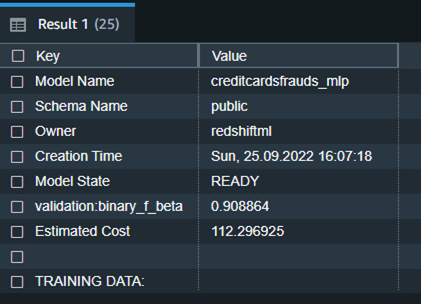
We notice from the preceding table that the F1-score for the training data is 0.908, which shows very good performance accuracy.

To elaborate, F1-score is the harmonic mean of precision and recall. It combines precision and recall into a single number using the following formula:

Where, Precision means: Of all positive predictions, how many are really positive?

And Recall means: Of all real positive cases, how many are predicted positive?

F1 scores can range from 0 to 1, with 1 representing a model that perfectly classifies each observation into the correct class and 0 representing a model that is unable to classify any observation into the correct class. So higher F1 scores are better.

The following is the detailed tabular outcome for the preceding command after model training was done.

Redshift ML now supports Prediction Probabilities for binary classification models. For classification problem in machine learning, for a given record, each label can be associated with a probability that indicates how likely this record really belongs to the label. With option to have probabilities along with the label, customers could use the classification results when confidence based on chosen label is higher than a certain threshold value returned by the model

Prediction probabilities are calculated by default for binary classification models and an additional function is created while creating model without impacting performance of the ML model.

In above snippet, you will notice that predication probabilities enhancements have added another function as a suffix (_prob) to model function with a name ‘creditcardsfrauds_mlp_fn_prob’ which could be used to get prediction probabilities.

Additionally, you can check the model explainability to understand which inputs contributed effectively to derive the prediction.

Model explainability helps to understand the cause of prediction by answering questions such as:

• Why did the model predict a negative outcome such as blocking of credit card when someone travels to a different country and withdraws a lot of money in different currency?
• How does the model make predictions? Lots of data for credit cards can be put in a tabular format and as per MLP process where a fully connected neural network of several layers is involved, we can tell which input feature actually contributed to the model output and its magnitude.
• Why did the model make an incorrect prediction? E.g. Why is the card blocked even though the transaction is legitimate?
• Which features have the largest influence on the behavior of the model? Is it just based upon the location where the credit card is swiped, or even the time of the day and unusual credit consumption that is influencing the prediction?

Run the following SQL command to retrieve the values from the explainability report:

SELECT json_table.report.explanations.kernel_shap.label0.global_shap_values 
FROM (select explain_model('creditcardsfrauds_mlp') as report) as json_table;

In the preceding screenshot, we have only selected the column that projects shapley values from the response returned by the explain_model function. If you notice the response of the query, the values in every json object show the contribution of different features in terms of influencing the prediction. E.g. from the preceding snippet, v14 feature is influencing the prediction the most and txtime feature does not really play any significant role in predicting ‘class’.

Model validation

Now let’s run the prediction query and validate the accuracy of the model on the validation dataset:

FROM (
  SELECT 
      CASE WHEN class =  
      creditcardsfrauds_mlp_fn(txtime,v1,v2,v3,v4,v5,v6,v7,v8,v9,v10,v11,v12,v13,v14,v15,v16,v17,v18,v19,v20,v21,v22,v23,v24,v25,v26,v27,v28,amount) 
      THEN 'PredictedMatchesActual' 
      else 'NoMatch' 
      END as actualvspredicted
    FROM creditcardsfrauds 
    WHERE txtime >= 120954
) 
group by actualvspredicted

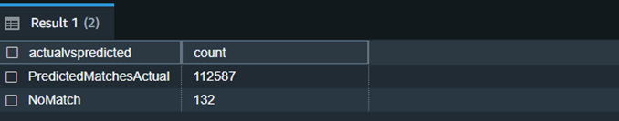
We can observe here that Redshift ML is able to identify 99.88 percent of the transactions correctly as fraudulent or non-fraudulent.

Now you can continue to use this SQL function creditcardsfrauds_mlp_fn for local inference in any part of the SQL query while analyzing, visualizing or reporting the newly arriving as well as existing data!

--CREATE A STAGING TABLE TO HOLD NEWLY ARRIVING DATA FROM THE SOURCE WHICH WILL NOT CONAIN THE CLASS COLUMN - AS IT IS TO BE PREDICTED
DROP TABLE creditcardsfrauds_staging;
CREATE TABLE creditcardsfrauds_staging as (select * from creditcardsfrauds limit 0);
Alter table creditcardsfrauds_staging drop column class;

--LETS CONSIDER ONLY ONE RECORD HERE WHICH HAS NEWLY ARRIVED
insert into creditcardsfrauds_staging values(174965,-39999.11383160738512,0.58586417180689,-5.39973021073242,1.81709247345531,-0.840618465991056,-2.94354779071974,-2.20800192003372,1.05873267723056,-1.63233334974982,-5000.24598383776964,11.93351953683592,-53046479695456,-1.12745457501155,-666666.41662797597451,0.141237234328704,-2.54949823633632,-4.61471706851594,-10.47813794126038,-0.0354803664667244,0.306270740368093,0.583275998701341,-0.269208637986581,-0.456107772584008,-0.183659129549716,-0.328167759255761,0.606115810329683,0.884875539542905,-0.253700318894381,-2450000000);

--USE THE FUNCTION TO PREDICT THE VALUE OF CLASS
SELECT txtime, creditcardsfrauds_mlp_fn(txtime,v1,v2,v3,v4,v5,v6,v7,v8,v9,v10,v11,v12,v13,v14,v15,v16,v17,v18,v19,v20,v21,v22,v23,v24,v25,v26,v27,v28,amount)
FROM creditcardsfrauds_staging;

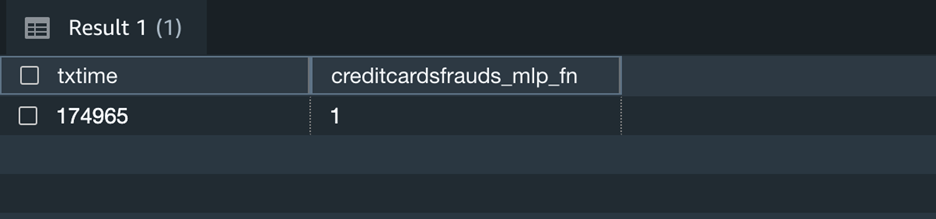
Here the output 1 means that the newly captured transaction is fraudulent as per the inference.

Additionally, you can change the above query to include prediction probabilities of label output for the above scenario and decide if you still like to use the prediction by the model.

--USE THE FUNCTION TO PREDICT THE VALUE OF CLASS ALONG WITH THE PROBABILITY
Select txtime, predictedActive.labels[0], predictedActive.probabilities[0] 
from (
SELECT txtime, creditcardsfrauds_mlp_fn_prob(txtime,v1,v2,v3,v4,v5,v6,v7,v8,v9,v10,v11,v12,v13,v14,v15,v16,v17,v18,v19,v20,v21,v22,v23,v24,v25,v26,v27,v28,amount)as predictedACtive
FROM creditcardsfrauds_staging ) temp

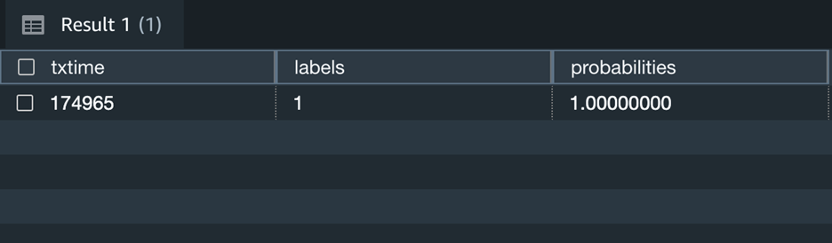
The above screenshot shows that this transaction has 100% likelihood of being fraudulent.

Clean up

To avoid incurring future charges, you can stop the Redshift cluster when not being used. You can even terminate the Redshift cluster altogether if you have run the exercise in this blog post just for experimental purpose. If you are instead using serverless version of Redshift, it will not cost you anything, until it is used. However, like mentioned before, you will have to stop or terminate the cluster if you are using a provisioned version of Redshift.

Conclusion

Redshift ML makes it easy for users of all levels to create, train, and tune models using SQL interface. In this post, we walked you through how to use the MLP algorithm to create binary classification model. You can then use those models to make predictions using simple SQL commands and gain valuable insights.

To learn more about RedShift ML, visit Amazon Redshift ML.

About the authors

Anuradha Karlekar is a Solutions Architect at AWS working majorly for Partners and Startups. She has over 15 years of IT experience extensively in full stack development, deployment, building data ETL pipelines and visualizations. She is passionate about data analytics and text search. Outside work – She is a travel enthusiast!

Phil Bates is a Senior Analytics Specialist Solutions Architect at AWS with over 25 years of data warehouse experience.

Abhishek Pan is a Solutions Architect-Analytics working at AWS India. He engages with customers to define data driven strategy, provide deep dive sessions on analytics use cases & design  scalable and performant Analytical applications. He has over 11 years of experience and is passionate about Databases, Analytics and solving customer problems with help of cloud solutions. An avid traveller and tries to capture world through my lenses

Debu Panda is a Senior Manager, Product Management at AWS, is an industry leader in analytics, application platform, and database technologies, and has more than 25 years of experience in the IT world. Debu has published numerous articles on analytics, enterprise Java, and databases and has presented at multiple conferences such as re:Invent, Oracle Open World, and Java One. He is lead author of the EJB 3 in Action (Manning Publications 2007, 2014) and Middleware Management (Packt).