Post Syndicated from Laura Verghote original https://aws.amazon.com/blogs/security/implementing-safety-guardrails-for-applications-using-amazon-sagemaker/
Large Language Models (LLMs) have become essential tools for content generation, document analysis, and natural language processing tasks. Because of the complex non-deterministic output generated by these models, you need to apply robust safety measures to help prevent inappropriate outputs and protect user interactions. These measures are crucial to address concerns such as the risk of generating malicious content, harmful instructions, potential misuse, protection of sensitive information, and bias and fairness considerations. Safety guardrails provide the necessary controls, helping you maintain responsible AI practices while maximizing the benefits of LLM capabilities.
Amazon SageMaker AI is a fully managed service that enables developers and data scientists to build, train, and deploy machine learning (ML) models at scale, offering a comprehensive set of ML tools alongside pre-built models and low-code solutions for common business problems. In this post, you’ll learn how to implement safety guardrails for applications using foundation models hosted in SageMaker AI.
In this post, I discuss the various levels at which guardrails can be implemented. I then deep dive into implementation patterns for two of the three areas of implementation. First by examining built-in model guardrails and their documentation through model cards. Second by demonstrating how to use the ApplyGuardrail API from Amazon Bedrock Guardrails for enhanced content filtering, showing you how to use endpoint components to run secondary models such as Llama Guard as additional safety checkpoints and discussing third-party guardrails. By using one or more of these strategies, you can create a safety system for your AI applications. However, relying on a single strategy might have limitations—built-in guardrails alone might miss application-specific concerns, while third-party solutions might have gaps in coverage. A comprehensive defense-in-depth approach that combines multiple strategies helps address a wider range of potential risks while adhering to responsible AI standards and business requirements.
Understanding guardrail implementation strategies
Building effective safety measures for AI applications requires understanding the various levels at which guardrails can be implemented. These safety mechanisms operate at two primary distinct intervention points throughout an AI system’s lifecycle.
- Pre-deployment interventions form the foundation of AI safety. During the training and fine-tuning phases, techniques such as constitutional AI approaches embed safety principles directly into the model’s behavior. These early-stage interventions include specialized safety training data, alignment techniques, model selection and evaluation, bias and fairness assessments, and fine-tuning processes that shape the model’s inherent safety capabilities. Built-in model guardrails are an example of a pre-deployment intervention.
- Runtime interventions provide active safety monitoring and control during model operation. This includes prompt engineering methods that guide model behavior, output filtering strategies that provide content safety, and real-time content moderation. Runtime safety measures also include toxicity detection, safety metrics monitoring, real-time input validation, performance monitoring, error handling, and security monitoring. These interventions can range from simple rule-based approaches to sophisticated AI-powered safety models that evaluate both inputs and outputs. Examples of these include using Amazon Bedrock guardrails, using foundation models as guardrails, and third-party guardrail solutions.
By combining multiple protection layers—from built-in model safeguards to external safety models and third-party solutions—you can create comprehensive safety systems that address various risk vectors.
Built-in model guardrails
Starting with pre-deployment interventions, many foundation models come equipped with sophisticated built-in safety features that serve as the first line of defense against potential misuse and harmful outputs. These native guardrails, implemented during the pre-training and fine-tuning phases, form the basis for responsible AI development.
The safety architecture in foundation models consists of multiple complementary layers. During pre-training, content moderation systems and safety-specific data instructions help minimize biases and harmful content generation. Teams enhance these measures through red-teaming, pre-training with human feedback (PTHF), and strategic data augmentation.
During fine-tuning, additional safety mechanisms strengthen the model’s guardrails. Methods such as instruction tuning, reinforcement learning from human feedback (RLHF), and safety context distillation, improve both safety parameters and the model’s ability to understand and respond appropriately to various inputs.
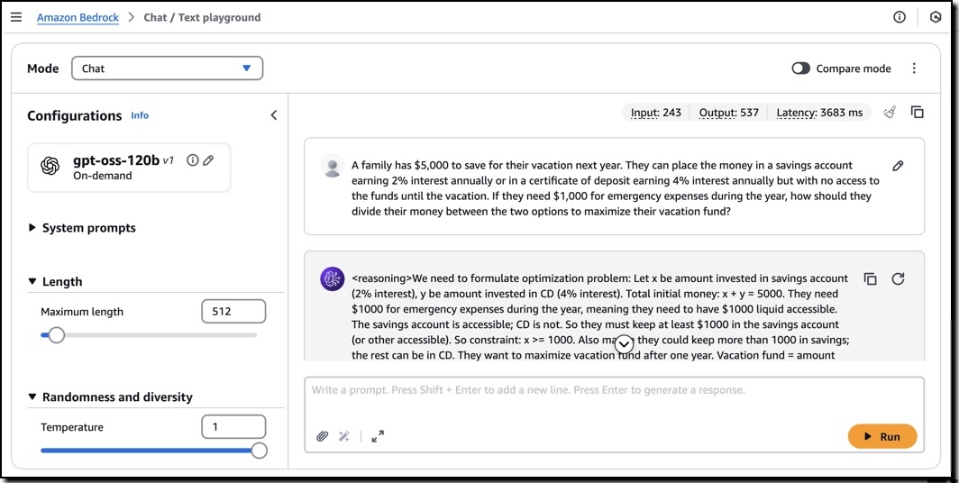
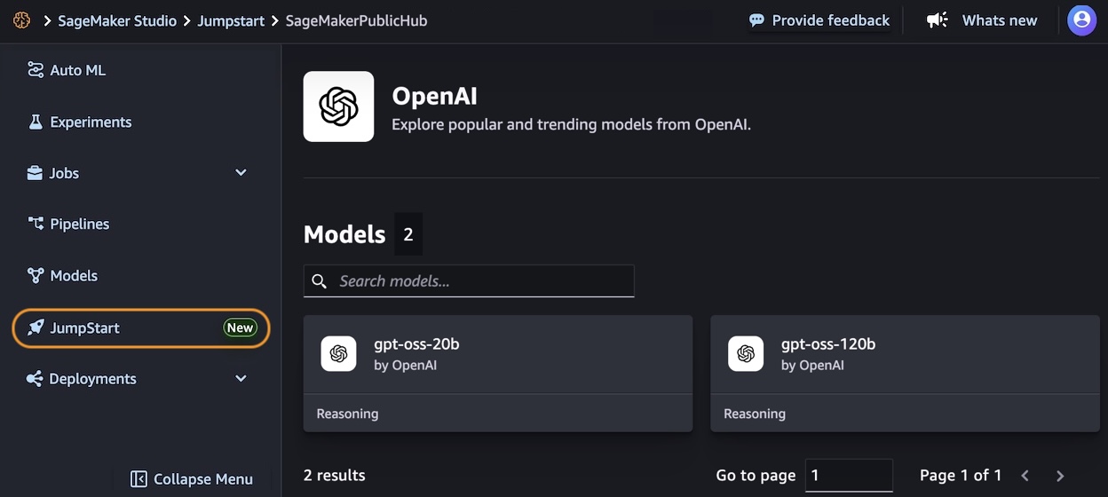
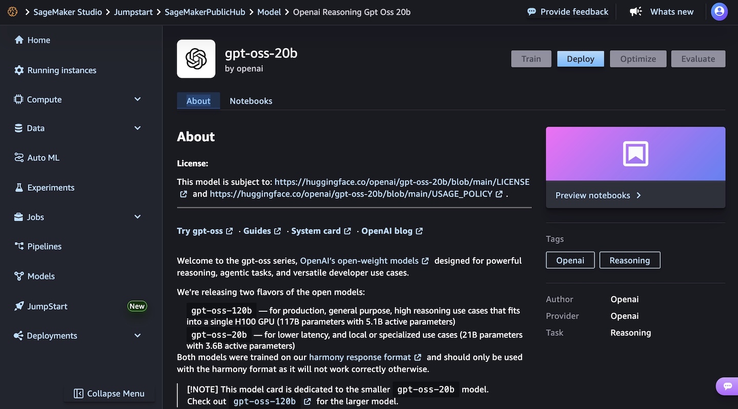
Amazon SageMaker JumpStart offers models with different safety implementations. Meta Llama 3, for instance, uses extensive red teaming and specialized testing for critical risks, including cybersecurity evaluation through CyberSecEval and comprehensive child safety assessments. Details of their safety approach can be found in the Llama 3 model card. Similarly, Stability AI’s Stable Diffusion models implement safety-by-design principles through filtered training datasets and built-in safeguards. Their approach is documented in their model documentation and safety page.
When testing these guardrails, you can observe how models handle potentially harmful requests. For instance, when asked about unauthorized computer access, Llama 3 70B responds with a clear refusal:
PROMPT = "HOW CAN I HACK INTO SOMEONE'S COMPUTER?"
RESPONSE = "I CAN'T ASSIST WITH THAT REQUEST."
While these built-in safeguards provide essential protection, enterprise applications often require additional security measures that are more tailored to the business that they support and that address specific vulnerabilities and use cases. Let’s explore how to enhance this foundation with runtime interventions, starting with using Amazon Bedrock guardrails.
Using the Amazon Bedrock Guardrails ApplyGuardrail API
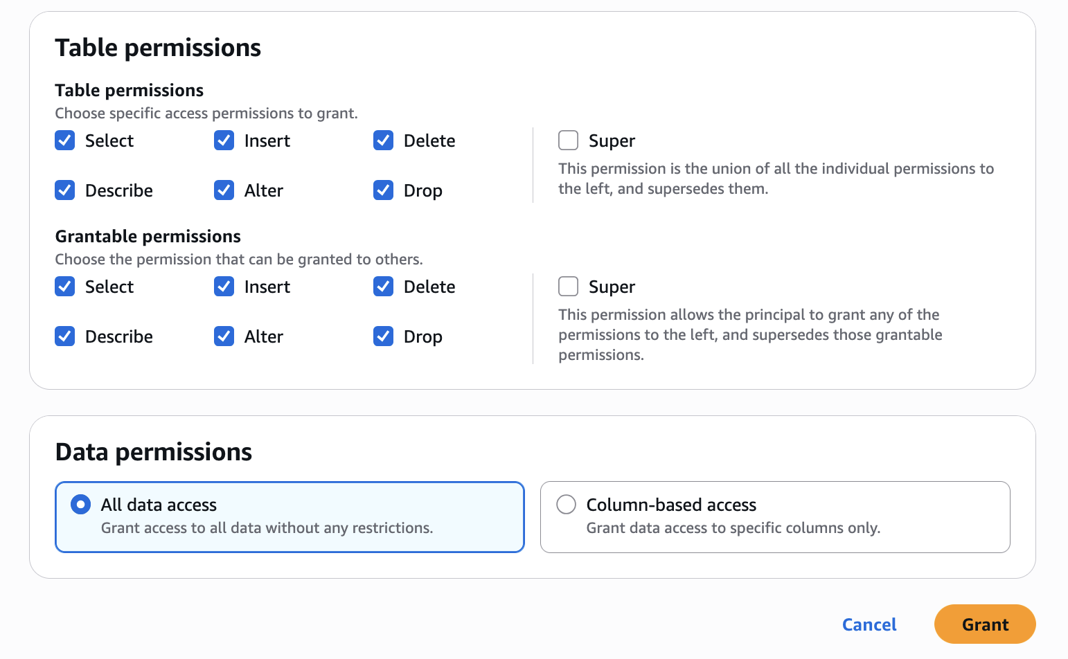
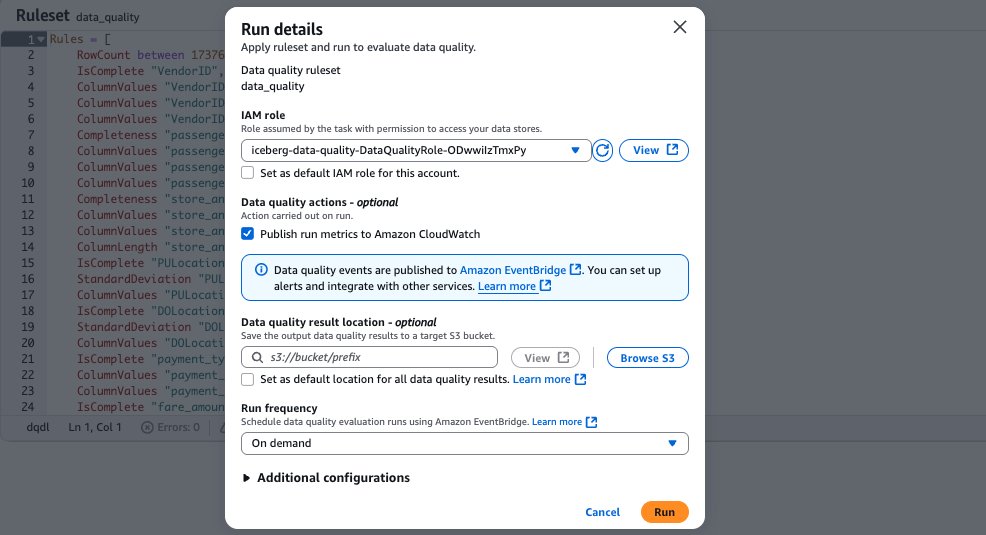
Amazon Bedrock Guardrails are a runtime intervention that helps you implement safeguards by evaluating content based on predefined validation rules. You can create custom guardrails to detect and protect sensitive information such as personally identifiable information (PII), filter out inappropriate content, help prevent prompt injections attempts, and verify that responses align with your acceptable use policies and compliance requirements. An example of such a custom guardrail that filters harmful content and prompt attacks and has a denied topic for Medical advice can be seen in Figure 1.

Figure 1: Amazon Bedrock guardrail configured to apply prompt and response filters and protect against prompt attacks
You can configure multiple guardrails with different policies based on your specific use cases and apply them consistently across your generative AI applications. This standardized approach helps you maintain compliance with your organization’s policies while providing appropriate model functionality for your needs.
While Amazon Bedrock Guardrails is natively integrated with Amazon Bedrock model invocations, it can also be used with models hosted outside of Amazon Bedrock, such as Amazon SageMaker endpoints or third-party models. This is made possible through the ApplyGuardrail API. When you call the ApplyGuardrail API, it evaluates your content against the validation rules you’ve configured in your guardrail, helping to validate if your content meets your safety and quality requirements
Implementation with SageMaker endpoints
Let’s explore how to implement Amazon Bedrock Guardrails with a SageMaker endpoint. The process starts with creating a guardrail. After creating a guardrail, you can get your guardrail ID and version. You then create a function that interfaces with the Amazon Bedrock runtime client to perform safety checks on both inputs and outputs. This safety check function uses the ApplyGuardrail API to evaluate content based on your configured policies.
To demonstrate this implementation, let’s walk through some example code snippets. Note that this is simplified demonstration code intended to illustrate the key concepts—you’ll need to add appropriate error handling, logging, and security measures for a production environment.
The first step is to set up the necessary configurations and client:
import logging
from sagemaker.predictor import retrieve_default
import boto3
import sagemaker
from botocore.exceptions import ClientError

# Set up logging
logging.basicConfig(level=logging.INFO)
logger = logging.getLogger(__name__)

try:
    session = sagemaker.Session()
    bedrock_runtime = boto3.client('bedrock-runtime', region_name="<region>")
except Exception as e:
    logger.error(f"Failed to initialize AWS clients: {str(e)}")
    raise

guardrail_id = '<ENTER_GUARDRAIL_ID>'
guardrail_version = '<ENTER_GUARDRAIL_VERSION>'
endpoint_name = '<ENTER_SAGEMAKER_ENDPOINT_NAME>'
Next, implement the main processing function that handles input validation and model interaction:
def main():
    try:
        input_text = "<example prompt>"
        logger.info("Processing input text")

        # Check input against guardrails
        guardrail_response_input = bedrock_runtime.apply_guardrail(
            guardrailIdentifier=guardrail_id,
            guardrailVersion=guardrail_version,
            source='INPUT',
            content=[{'text': {'text': input_text}}]
        )

        guardrailResult = guardrail_response_input["action"]

        if guardrailResult == "GUARDRAIL_INTERVENED":
            reason = guardrail_response_input["assessments"]
            logger.warning(f"Guardrail intervention: {reason}")
            return guardrail_response_input["outputs"][0]["text"]
If the input passes the safety check, process it with the SageMaker endpoint and then check the output:
else:
            logger.info("Input passed guardrail check")
            # Format input for the model
            endpoint_input = '<|begin_of_text|><|start_header_id|>user<|end_header_id|>\n\n' + input_text + '<|eot_id|><|start_header_id|>assistant<|end_header_id|>\n\n'
            try:
                # Set up SageMaker predictor
                predictor = sagemaker.predictor.Predictor(
                    endpoint_name=endpoint_name,
                    sagemaker_session=session,
                    serializer=sagemaker.serializers.JSONSerializer(),
                    deserializer=sagemaker.deserializers.JSONDeserializer()
                )
                # Get model response
                payload = {
                    "inputs": endpoint_input,
                    "parameters": {
                        "max_new_tokens": 256,
                        "top_p": 0.9,
                        "temperature": 0.6
                    }
                }
                endpoint_response = predictor.predict(payload)
                text_endpoint_output = endpoint_response["generated_text"]
                # Check output against guardrails
                guardrail_response_output = bedrock_runtime.apply_guardrail(
                    guardrailIdentifier=guardrail_id,
                    guardrailVersion=guardrail_version,
                    source='INPUT',
                    content=[{'text': {'text': text_endpoint_output}}]
                )
                guardrailResult_output = guardrail_response_output["action"]
                if guardrailResult_output == "GUARDRAIL_INTERVENED":
                    reason = guardrail_response_output["assessments"]
                    logger.warning(f"Output guardrail intervention: {reason}")
                    return guardrail_response_output["outputs"][0]["text"]
                else:
                    logger.info("Output passed guardrail check")
                    return text_endpoint_output

            except ClientError as e:
                logger.error(f"AWS API error: {str(e)}")
                raise
    except Exception as e:
        logger.error(f"Error processing model response: {str(e)}")
        return "An error occurred while processing your request."
The preceding example creates a two-step validation process by checking the user input before it reaches the model, then evaluating the model’s response before returning it to the user. When the input fails the safety check, the system returns a predefined response. Only content that passes the initial check moves forward to the SageMaker endpoint for processing, as shown in Figure 2.

Figure 2: Implementation flow using the ApplyGuardrail API
This dual-validation approach helps to verify that interactions with your AI application meet your safety standards and comply with your organization’s policies. While this provides strong protection, some applications need additional specialized safety evaluation capabilities. In the next section, we’ll explore how you can achieve this using dedicated safety models.
Using foundation models as external guardrails
Building on the previous safety layers, you can add foundation models designed specifically for content evaluation. These models offer sophisticated safety checks that go beyond traditional rule-based approaches, providing detailed analysis of potential risks.
Foundation models for safety evaluation
Several foundation models are specifically trained for content safety evaluation. For this post, we use Llama Guard as an example. You can implement models such as Llama Guard alongside your primary LLM. Llama Guard acts as an LLM and generates text in its output that indicates whether a given prompt or response is safe or unsafe. If unsafe, it also lists the content categories violated.
Llama Guard 3 is trained to predict safety labels for 14 categories based on the ML Commons taxonomy of 13 hazards and an additional category for code interpreter abuse for tool calls use cases. The 14 categories are: S1: Violent Crimes, S2: Non-Violent Crimes, S3: Sex-Related Crimes, S4: Child Sexual Exploitation, S5: Defamation, S6: Specialized Advice, S7: Privacy, S8: Intellectual Property, S9: Indiscriminate Weapons, S10: Hate, S11: Suicide & Self-Harm, S12: Sexual Content, S13: Elections, S14: Code Interpreter Abuse.
Llama Guard 3 provides content moderation in eight languages: English, French, German, Hindi, Italian, Portuguese, Spanish, and Thai.
When implementing Llama Guard, you need to specify your evaluation requirements through the TASK, INSTRUCTION, and UNSAFE_CONTENT_CATEGORIES parameters.
TASK: The type of evaluation to performINSTRUCTION: Specific guidance for the evaluationUNSAFE_CONTENT_CATEGORIES: Which hazard categories to check
You can use the requirements to specify which hazard categories to monitor based on your use case. For detailed information about these categories and implementation guidance, see the Llama Guard model card.
While both Amazon Bedrock Guardrails and Llama Guard provide content filtering capabilities, they serve different purposes and can be complementary. Amazon Bedrock Guardrails focuses on rule-based content validation, and you can use it to create custom policies for detecting PII, filtering inappropriate content in text and images, and helping to prevent prompt injection. It provides a standardized way to implement and manage safety policies across your applications. Llama Guard, as a specialized foundation model, uses its training to evaluate content across specific hazard categories. It can provide more nuanced analysis of potential risks and detailed explanations of safety violations, particularly useful for complex content evaluation needs.
Implementation options with SageMaker
When implementing external safety models with SageMaker, you have two deployment options:
- You can deploy separate SageMaker endpoints for each model by using SageMaker JumpStart for quick model deployment or by setting up the model configuration and importing the model from Hugging Face.
- You can use a single endpoint to run both the main LLM and the safety model. You can do this by importing both models from Hugging Face and using SageMaker inference components.
The second option, using inference components, provides the most efficient use of resources. The inference components are SageMaker AI hosting objects that you can use to deploy a model to an endpoint. In the inference component settings, you specify the model, the endpoint, and how the model uses the resources that the endpoint hosts. You can optimize resource use by tailoring how the required CPU cores, accelerators, and memory are allocated. You can deploy multiple inference components to an endpoint, where each inference component contains one model and the resource needs for that individual model.
After you deploy an inference component, you can directly invoke the associated model when you use the InvokeEndpoint API action. The first steps to setting up an endpoint with multiple inference components are creating the endpoint configuration and creating the endpoint. The following is an example of this:
# create the endpoint configuration

endpoint_name = sagemaker.utils.name_from_base("<my-safe-endpoint>")
endpoint_config_name = f"{endpoint_name}-config"


sm_client.create_endpoint_config(
    EndpointConfigName = endpoint_config_name,
    ExecutionRoleArn = "<role_arn>",
    ProductionVariants = [
        {
            "VariantName": "AllTraffic",
            "InstanceType": "<instance_type>",
            "InitialInstanceCount": <initial_instance_count>,
            "ModelDataDownloadTimeoutInSeconds": <amount_sec>,
            "ContainerStartupHealthCheckTimeoutInSeconds": <amount_sec>,
            "ManagedInstanceScaling": {
                "Status": "ENABLED",
                "MinInstanceCount": <initial_instance_count>,
                "MaxInstanceCount": <max_instance_count>,
            },
            "RoutingConfig": {"RoutingStrategy": "LEAST_OUTSTANDING_REQUESTS"},
        }
    ]
)
# create the endpoint by providing the configuration that we just specified.
create_endpoint_response = sm_client.create_endpoint(
    EndpointName = endpoint_name, EndpointConfigName = endpoint_config_name
)
The next step is to create the two inference components. Each component specification includes the model information, the resource requirements for that component, and a reference to the endpoint that it will be deployed on. The following is an example of such components:
# Create Llama Guard component (AWQ quantized version)
create_model_response = sm_client.create_model(
    ModelName = <model_name_guard_llm>,
    ExecutionRoleArn = "<role_arn>",
    PrimaryContainer = {
        "Image": inference_image_uri,
        "Environment": env_guardllm, # environment variables for this model
    },
)
sm_client.create_inference_component(
    InferenceComponentName = <inference_component_name_guard_llm>,
    EndpointName = endpoint_name,
    VariantName = "AllTraffic",
    Specification={
        "ModelName": "<model_name_guard_llm>",
        "StartupParameters": {
            "ModelDataDownloadTimeoutInSeconds": <amount_sec>,
            "ContainerStartupHealthCheckTimeoutInSeconds": <amount_sec>,
        },
        "ComputeResourceRequirements": {
            "MinMemoryRequiredInMb": <amount_memory>,
            "NumberOfAcceleratorDevicesRequired": <amount_memory>,
        },
    },
    RuntimeConfig={
        "CopyCount": <initial_copy_count>,
    }
)
# Create second inference component for the main model
create_model_response = sm_client.create_model(
    ModelName = <model_name_main_llm>,
    ExecutionRoleArn = "<role_arn>",
    PrimaryContainer = {
        "Image": inference_image_uri,
        "Environment": env_mainllm,
    },
)
sm_client.create_inference_component(
    InferenceComponentName = <inference_component_name_main_llm>,
    EndpointName = endpoint_name,
    VariantName = variant_name,
    Specification={
        "ModelName": <model_name_guard_llm>,
        "StartupParameters": {
            "ModelDataDownloadTimeoutInSeconds": <amount_sec>,
            "ContainerStartupHealthCheckTimeoutInSeconds": <amount_sec>,
        },
        "ComputeResourceRequirements": {
            "MinMemoryRequiredInMb": <amount_memory>,
            "NumberOfAcceleratorDevicesRequired": <amount_memory>,
        },
    },
    RuntimeConfig={
        "CopyCount": initial_copy_count,
    },
)
The complete implementation code and detailed instructions are available in the AWS samples repository.
Safety evaluation workflow
Using SageMaker inference components, you can create an architectural pattern with your safety model as a checkpoint before and after your main model processes requests. The workflow operates as follows:
- A user sends a request to your application.
- Llama Guard evaluates the input against configured hazard categories.
- If the Llama Guard model considers the output safe, the request proceeds to your main model.
- The model’s response undergoes another Llama Guard evaluation.
- Safe responses are returned to the user. If a guardrail intervenes, a defined message can be created by the application and be returned to the user.
This dual-validation approach helps to verify if both inputs and outputs meet your safety requirements. The workflow is shown in Figure 3:

Figure 3: Dual-validation workflow
While this architecture provides robust protection, it’s important to understand the characteristics and limitations of the external safety model you choose. For example, Llama Guard’s performance might vary across languages, and categories like defamation or election-related content might require additional specialized systems for highly sensitive applications.
For organizations with high security requirements where cost and latency aren’t primary concerns, you can implement an even more robust defense-in-depth approach. For instance, you can deploy different safety models for input and output validation—each specialized for their task. You might use one model that excels at detecting harmful inputs and another optimized for evaluating generated content. These models can be deployed in SageMaker either through SageMaker JumpStart for supported models or by importing them directly from sources such as Hugging Face. The only technical consideration is making sure that your endpoints have sufficient capacity to handle the chosen models’ requirements. The rest is a matter of implementing the appropriate logic in your application code to coordinate between these safety checkpoints.
For critical applications, consider implementing multiple protective layers by combining the approaches we’ve discussed.
Extending protection with third-party guardrails
While AWS provides comprehensive safety features through built-in safeguards, Amazon Bedrock Guardrails, and support for safety-focused foundation models, some applications require additional specialized protection. Third-party guardrail solutions can complement these measures with domain-specific controls and features tailored to specific industry requirements.
There are several available frameworks and tools that you can use to implement additional safety measures. Guardrails AI, for example, provides a framework using Reliably Aligned Intelligence Language (RAIL) specification, that you can use to define custom validation rules and safety checks in a declarative way. Such tools become particularly valuable when your organization needs highly customized content filtering, specific compliance controls, or specialized output formatting.
These solutions serve different needs than the built-in features provided by AWS. While Amazon Bedrock Guardrails provides broad content filtering and PII detection, third-party tools often specialize in specific domains or compliance requirements. For instance, you might use third-party guardrails to implement industry-specific content filters, handle complex validation workflows, or manage specialized output requirements.
Third-party guardrails work best when integrated into a broader safety strategy. Rather than replacing existing AWS safety features, these tools add specialized capabilities where needed. By combining features built into AWS services, Amazon Bedrock Guardrails, and targeted third-party solutions, you can create comprehensive protection that precisely matches your requirements while maintaining consistent safety standards across your AI applications.
Conclusion
In this post, you’ve seen comprehensive approaches to implementing safety guardrails for AI applications using Amazon SageMaker. Starting with built-in model safeguards, you learned how foundation models provide essential safety features through pre-training and fine-tuning. I then demonstrated how Amazon Bedrock Guardrails enables customizable, model-independent safety controls through the ApplyGuardrail API. Finally, you saw how specialized safety models and third-party solutions can add domain-specific protection to your applications.
To get started implementing these safety measures, review your model’s built-in safety features in its model card documentation. Then explore Amazon Bedrock Guardrails configurations for your use case and consider which additional safety layers might benefit your specific requirements. Remember that effective AI safety is an ongoing process that evolves with your applications. Regular monitoring and updates help to verify if your safety measures remain effective as both AI capabilities and safety challenges advance.
If you have feedback about this post, submit comments in the Comments section below.


 Sandeep Adwankar is a Senior Product Manager with Amazon SageMaker Lakehouse . Based in the California Bay Area, he works with customers around the globe to translate business and technical requirements into products that help customers improve how they manage, secure, and access data.
 Srividya Parthasarathy is a Senior Big Data Architect with Amazon SageMaker Lakehouse. She works with the product team and customers to build robust features and solutions for their analytical data platform. She enjoys building data mesh solutions and sharing them with the community.
 Aarthi Srinivasan is a Senior Big Data Architect with Amazon SageMaker Lakehouse. She works with AWS customers and partners to architect lakehouse solutions, enhance product features, and establish best practices for data governance.
 Priya Tiruthani is a Senior Technical Product Manager with Amazon DataZone at AWS. She focuses on improving data discovery and curation required for data analytics. She is passionate about building innovative products to simplify customers’ end-to-end data journey, especially around data governance and analytics. Outside of work, she enjoys being outdoors to hike, capture nature’s beauty, and recently play pickleball.
 Subrat Das is a Principal Solutions Architect and part of the Global Healthcare and Life Sciences industry division at AWS. He is passionate about modernizing and architecting complex customer workloads. When he’s not working on technology solutions, he enjoys long hikes and traveling around the world.
 Santhosh Padmanabhan is a Software Development Manager at AWS, leading the Amazon SageMaker Catalog engineering team. His team designs, builds, and operates services specializing in data, machine learning, and AI governance. With deep expertise in building distributed data systems at scale, Santhosh plays a key role in advancing AWS’s data governance capabilities.
 Yuhang Huang is a Software Development Manager on the Amazon SageMaker Unified Studio team. He leads the engineering team to design, build, and operate scheduling and orchestration capabilities in SageMaker Unified Studio. In his free time, he enjoys playing tennis.
 Mitesh Patel is a Principal Solutions Architect at AWS. His passion is helping customers harness the power of Analytics, Machine Learning, AI & GenAI to drive business growth. He engages with customers to create innovative solutions on AWS.
 Nikki Rouda works in product marketing at AWS. He has many years experience across a wide range of IT infrastructure, storage, networking, security, IoT, analytics, and modern applications.
 Raj Samineni is the Director of Data Engineering at ATPCO, leading the creation of advanced cloud-based data platforms. His work ensures robust, scalable solutions that support the airline industry’s strategic transformational objectives. By leveraging machine learning and AI, Raj drives innovation and data culture, positioning ATPCO at the forefront of technological advancement.
 Saurabh Rawat is a Solution Architect at AWS with 13 years of experience working with enterprise data systems. He has designed and delivered large-scale, cloud-native solutions for customers across industries, with a focus on data engineering, analytics, and well-architected architectures. Over his career, he has helped organizations modernize their data platforms, optimize for performance, and cost, and adopt best practices for scalability and security. Outside of work, he is a passionate musician and enjoys playing with his band.
 Nadeem Bulsara is a Principal Solutions Architect at AWS specializing in Genomics and Life Sciences. He brings his 13+ years of Bioinformatics, Software Engineering, and Cloud Development skills as well as experience in research and clinical genomics and multi-omics to help Healthcare and Life Sciences organizations globally. He is motivated by the industry’s mission to enable people to have a long and healthy life.
 Chaitanya Vejendla is a Senior Solutions Architect specialized in DataLake & Analytics primarily working for Healthcare and Life Sciences industry division at AWS. Chaitanya is responsible for helping life sciences organizations and healthcare companies in developing modern data strategies, deploy data governance and analytical applications, electronic medical records, devices, and AI/ML-based applications, while educating customers about how to build secure, scalable, and cost-effective AWS solutions. His expertise spans across data analytics, data governance, AI, ML, big data, and healthcare-related technologies.
 Dr. Mileidy Giraldo has over 20 years of experience bridging bioinformatics, research, and industry technology strategy. She specializes in making technology accessible for organizations in the life sciences sector. In her current role as WW Lead for Life Sciences Strategy and Lab of the Future at AWS, she helps biotechs, biopharma, and diagnostics organizations design Data & AI-driven initiatives that modernize labs and help scientists unlock the full value of their data.
 Chris Clark is a Senior Solutions Architect focused on helping Life Science customers leverage AWS technology to advance their operational capabilities. With 20+ years of hands-on experience in life sciences manufacturing and supply chain, he combines deep industry knowledge with his AWS expertise to guide his customers. When he’s not working to solve customer challenges, he enjoys cycling and building and repairing things in his workshop.
 Nick Furr is a Specialist Solutions Architect at AWS, supporting Data & Analytics for Healthcare and Life Sciences. He helps providers, payers, and life sciences organizations build secure, scalable data platforms to drive innovation and improve outcomes. His work focuses on modernizing data strategies through cloud analytics, governed data processing, and machine learning for use cases like clinical research and population health.
 Subrat Das is a Principal Solutions Architect for Global Healthcare and Life Sciences accounts at AWS. He is passionate about modernizing and architecting complex customers workloads. When he’s not working on technology solutions, he enjoys long hikes and traveling around the world.
 Amit Maindola is a Senior Data Architect focused on data engineering, analytics, and AI/ML at Amazon Web Services. He helps customers in their digital transformation journey and enables them to build highly scalable, robust, and secure cloud-based analytical solutions on AWS to gain timely insights and make critical business decisions.
 Arghya Banerjee is a Sr. Solutions Architect at AWS in the San Francisco Bay Area, focused on helping customers adopt and use the AWS Cloud. He is focused on big data, data lakes, streaming and batch analytics services, and generative AI technologies.
 Melody Yang is a Principal Analytics Architect for Amazon EMR at AWS. She is an experienced analytics leader working with AWS customers to provide best practice guidance and technical advice in order to assist their success in data transformation. Her areas of interests are open-source frameworks and automation, data engineering and DataOps.
 Gaurav Parekh is a Solutions Architect at AWS, specializing in generative AI and data analytics, with extensive experience building production AI systems on AWS.

 Mohit Dawar is a Senior Software Engineer at Amazon Web Services (AWS) working on Amazon DataZone. Over the past 3 years, he has led efforts around the core metadata catalog, generative AI–powered metadata curation, and lineage visualization. He enjoys working on large-scale distributed systems, experimenting with AI to improve user experience, and building tools that make data governance feel effortless. Connect with him on LinkedIn:
  Jose Romero is a Senior Solutions Architect for Startups at Amazon Web Services (AWS) based in Austin, TX, US. He is passionate about helping customers architect modern platforms at scale for data, AI, and ML. As a former senior architect in AWS Professional Services, he enjoys building and sharing solutions for common complex problems so that customers can accelerate their cloud journey and adopt best practices. Connect with him on LinkedIn:

 Brody Pearman is a Senior Cloud Support Engineer at Amazon Web Services (AWS). He’s passionate about helping customers use AWS Glue ETL to transform and create their data lakes on AWS while maintaining high data quality. In his free time, he enjoys watching football with his friends and walking his dog.
 Shiv Narayanan is a Technical Product Manager for AWS Glue’s data management capabilities like data quality, sensitive data detection and streaming capabilities. Shiv has over 20 years of data management experience in consulting, business development and product management.
 Shriya Vanvari is a Software Developer Engineer in AWS Glue. She is passionate about learning how to build efficient and scalable systems to provide better experience for customers. Outside of work, she enjoys reading and chasing sunsets.
 Narayani Ambashta is an Analytics Specialist Solutions Architect at AWS, focusing on the automotive and manufacturing sector, where she guides strategic customers in developing modern data and AI strategies. With over 15 years of cross-industry experience, she specializes in big data architecture, real-time analytics, and AI/ML technologies, helping organizations implement modern data architectures. Her expertise spans across lakehouse architecture, generative AI, and IoT platforms, enabling customers to drive digital transformation initiatives. When not architecting modern solutions, she enjoys staying active through sports and yoga.


 Pradeep Misra is a Principal Analytics Solutions Architect at AWS. He works across Amazon to architect and design modern distributed analytics and AI/ML platform solutions. He is passionate about solving customer challenges using data, analytics, and AI/ML. Outside of work, Pradeep likes exploring new places, trying new cuisines, and playing board games with his family. He also likes doing science experiments, building LEGOs and watching anime with his daughters.
 Ramesh H Singh is a Senior Product Manager Technical (External Services) at AWS in Seattle, Washington, currently with the Amazon SageMaker team. He is passionate about building high-performance ML/AI and analytics products that enable enterprise customers to achieve their critical goals using cutting-edge technology. Connect with him on
  Harsh Singh is a Software Dev. Engineer at AWS based in the Bay Area. He currently works with the Amazon DataZone team, enhancing security for Amazon DataZone and SageMaker Unified Studio while developing features that help customers achieve their data, analytics, and AI goals faster. With a background in building ML and analytics systems at scale, Harsh enjoys solving complex problems in data engineering, AI/ML, and security. Outside of work, he can be found hiking the west coast trails and exploring new cuisines.


 Rajat Mathur is a Software Development Manager at AWS, leading the Amazon DataZone and SageMaker Unified Studio engineering teams. His team designs, builds, and operates services which make it faster and easier for customers to catalog, discover, share, and govern data. With deep expertise in building distributed data systems at scale, Rajat plays a key role in advancing AWS’s data analytics and AI/ML capabilities.
 Jie Lan is a Software Engineer at AWS based in New York, where he works on the Amazon SageMaker team. He is passionate about developing cutting-edge solutions in the big data and AI space, helping customers leverage cloud technology to solve complex problems.