Post Syndicated from Arash Rowshan original https://aws.amazon.com/blogs/big-data/estimating-scoring-probabilities-by-preparing-soccer-matches-data-with-aws-glue-databrew/

In soccer (or football outside of the US), players decide to take shots when they think they can score. But how do they make that determination vs. when to pass or dribble? In a fraction of a second, in motion, while chased from multiple directions by other professional athletes, they think about their distance from the goal, the speed they’re running, the ball movement, the number of defenders, the goalkeeper’s position, their own shot power, accuracy, angle, and more. For a moment, time stands still. A decision is made. To shoot or not to shoot.

This post was inspired by AWS’s collaboration with Germany’s Bundesliga, which lead to Match Fact xGoals. We use representative sample datasets and walk through using AWS Glue DataBrew to prepare data prior to training a model that can predict the probability of a player scoring at any given moment in the game.

We start with two datasets that have the information about the events in the game and the players. We describe how a problem in this domain could be framed to benefit from data preparation and how that can lead us to making predictions.

No prior knowledge is required to enjoy this post. However, basic familiarity with data preparation and machine learning (ML) is beneficial. By the end of this post, you should have a good sense regarding what DataBrew offers as well as how you can apply the approaches offered here to other use cases.

Sample datasets

Let’s assume we have collected a lot of data from video records of soccer matches. We extracted the following dataset by taking a snapshot of every shot taken in every match. For each shot, we also recorded if it resulted in a goal or if it did not. The dataset is fictionalized and not based on historic soccer games.

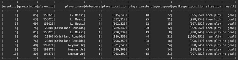
The following table summarizes what each column contains.

Column Name	Description
event_id	Unique identifier for each record
game_minute	Minute of the game between 0 to approximately 90
player_id	Unique identifier for each player
player_name	Name of the player who took the shot
defenders	Number of defenders between the player and the opponent’s goalkeeper
player_position	[x, y] coordinate of the player taking the shot
player_angle	Angle of the player taking the shot
player_speed	Speed of the player at the moment taking the shot in km/h
goalkeeper_position	[x, y] coordinate of the opponent’s goalkeeper
situation	Open play, free kick, or penalty kick
result	Goal or no goal

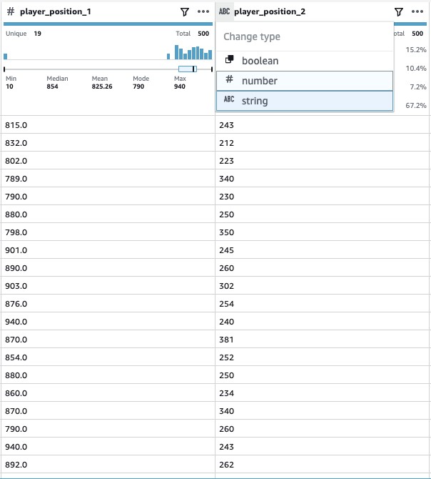
We also use the FIFA 20 complete player dataset, a dataset on soccer players across the globe that attempts to estimate their qualities quantitatively. The following screenshot shows some of the columns this dataset contains.

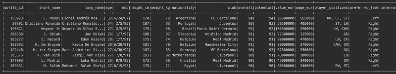
We’re interested in the following columns:

• age
• height
• weight
• overall
• preferred_foot
• weak_foot
• pace
• shooting
• attacking_finishing
• skill_fk_accuracy
• movement_acceleration
• movement_sprint_speed
• power_shot_power
• mentality_penalties 

We talk more about how each of these columns can be relevant later in this post.

As you can imagine, these datasets aren’t quite ready to train an ML model. We need to combine, clean, and extract values in numeric forms so we can start creating our training set. Normally that can take a lot of time and is somewhat tedious work. Data scientists prefer to focus on training their model, but they have to spend most of their time wrangling data to the shape that can be used for their ML flow.

But fear not! Enter AWS Glue DataBrew, your friendly neighborhood visual data prep tool. As businesswire puts it, “

“…AWS Glue DataBrew offers customers over 250 pre-built transformations to automate data preparation tasks that would otherwise require days or weeks writing hand-coded transformations.”

Let’s get to work and see how we can prepare a dataset for training an ML model using DataBrew.

Preparing the data with DataBrew

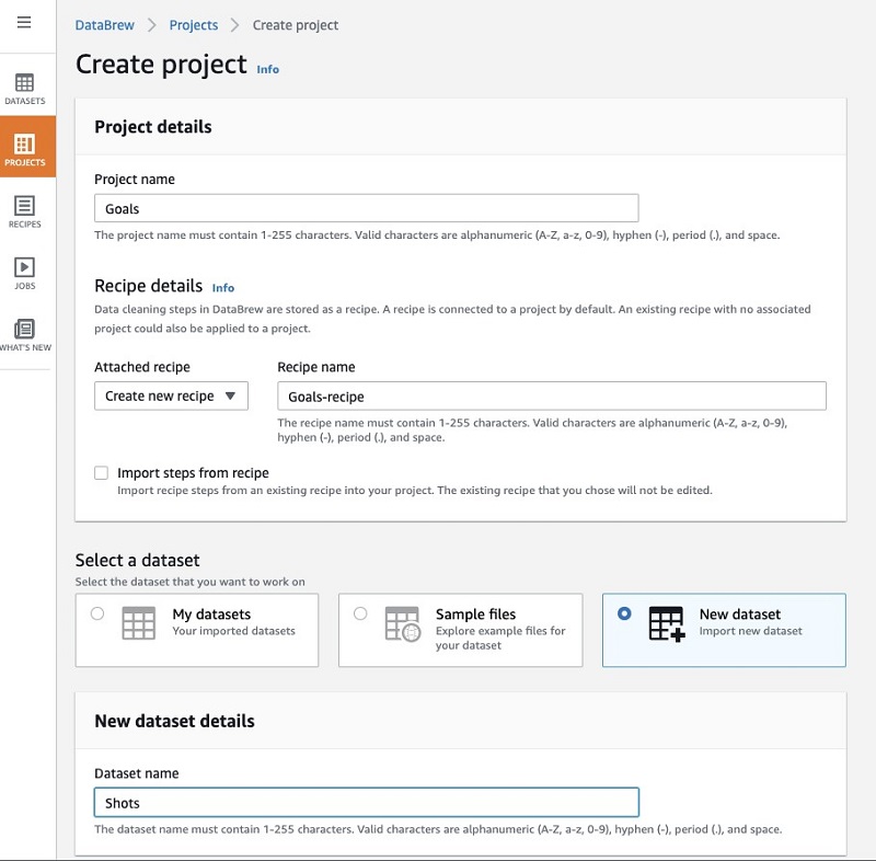
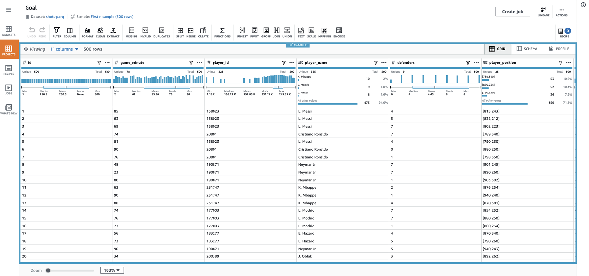
Let’s start with the shots dataset. I first create a project on the DataBrew console and upload this dataset.

When my session is ready, I should see all the columns and some analytics that give me useful insights about my dataset.

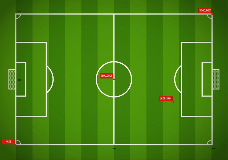
The player_position column is recorded as [x,y] coordinates with x between 0–1000 and y between 0–500. The following image shows how a player is positioned based on this data.

In CSV, this is recorded as a string and has two values. We want to extract the values and combine them into a single value that can be represented as a number. This can help our model draw better conclusions from this feature. We can start preparing our data by completing the following steps:

1. Using the Remove values transform, I remove the opening and closing brackets from the entries of the player_position column.

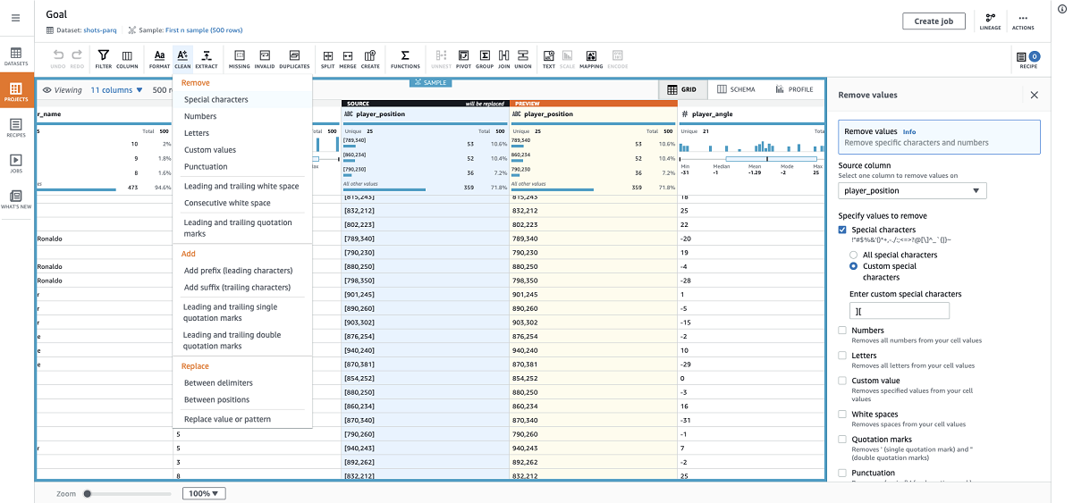
2. I split this column by a comma to generate two columns that hold the x and y coordinates.

3. We also need to convert these newly generated columns from strings to numbers.

Now we can generate a single value using the two columns that we generated. Imagine we want to break down the whole soccer field into 1×1 squares. If we think about the field similar to rows and columns, we can calculate the number for each square as such: x * 500 + y.

The benefit of this approach is that squares with higher numbers tend to be closer to the opponent’s goal, and this single feature can help our model draw good correlations between a player’s location and event outcomes. Note that the squares in the following image aren’t drawn to scale.

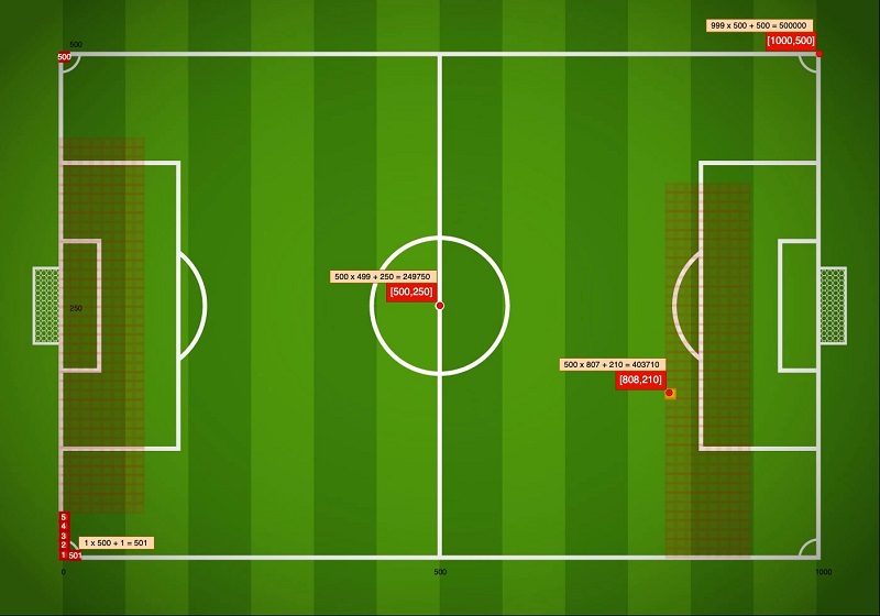
We can calculate the square numbers by using the the Functions transform Multiply and then Sum.

4. First I multiple the x coordinate by 500.

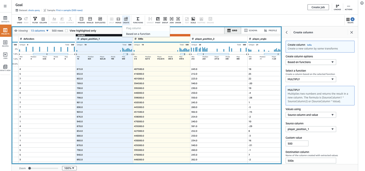
5. Using the ADD function, I sum this generated column with the y coordinate.

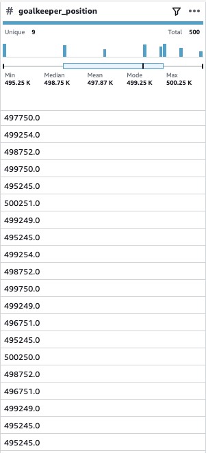
6. We apply the same transforms to the goal_keeper position to achieve a single number for that feature as well.

Next, let’s take a look at the player_angle column.

When positioned on the lower half of the field, a positive angle likely presents a better opportunity to score, and when on the top half, a negative angle faces the players more toward the goal. Another point to consider is the player’s strong or weak foot. The bottom half presents a wide angle for a left-footed player and the top half does so for a right-footed player. Angle in combination with strong foot can help our model draw good conclusions. We add the information on players’ strong or weak foot later in this post.

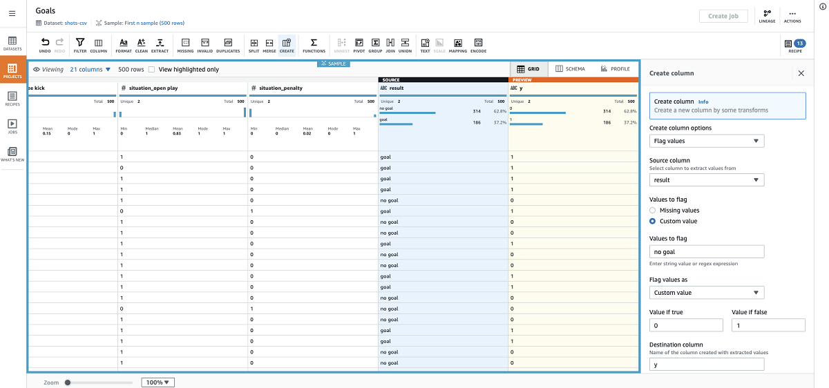
We have three different situations recorded in our dataset.

7. We apply one-hot-encoding to this column to refactor the situations as 1 (True) or 0 (False) values suitable for training our model.

8. For the shots dataset, we change the results column to 0s and 1s using the custom flag transform.
9. Because this is what we want to predict, I name the column y.

We can enrich the data further by joining this dataset with the player dataset to take each player’s qualities into consideration. You may have noticed that we generated a lot of extra columns while applying the previous transforms. We can address that in one step while we do the join and clean things up a bit.

10. When applying the join, we can connect the players dataset.

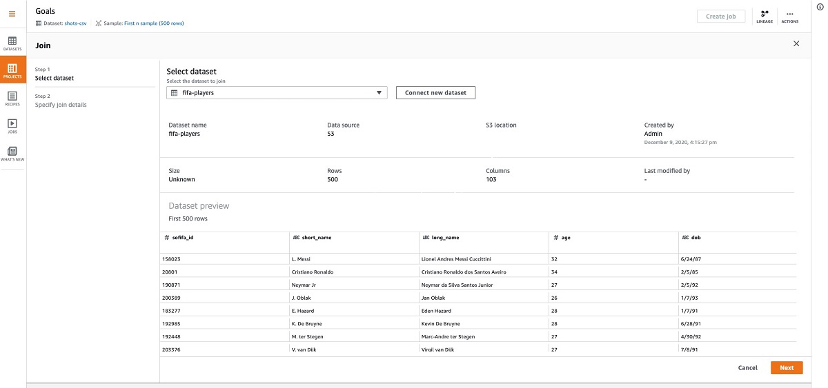
11. I use an inner join and choose player_id as my key.
12. I also only select the columns that I’m interested in.

You can select more or fewer columns depending on what features you want to feed into your model. For instance, I’m not selecting the player’s nationality, but you may want your model to take that into consideration. That’s really up to you, so feel free to play around with your options.

13. I deselect the extra columns from the shots dataset and only select the following from the players dataset:
    1. age
    2. overall
    3. preferred_foot
    4. weak_foot
    5. shooting
    6. attacking_finishing
    7. skill_fk_accuracy
    8. movement_acceleration
    9. movement_sprint_speed
    10. power_shot_power
    11. mentality_penalties 

We’re almost done. We just need to apply a few transforms to the newly added player columns.

14. I one-hot-encode preferred foot.

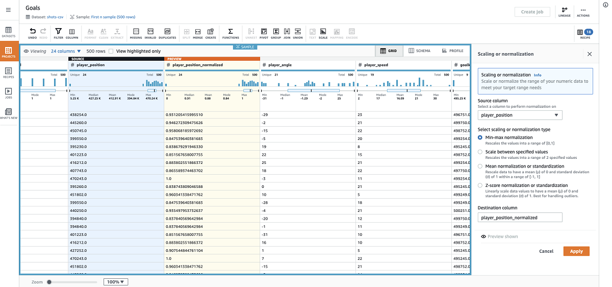
We can normalize some of the columns depending on the ML model that we want to run on this dataset afterwards. I want to train a basic logistic regression model.

15. I use min-max normalization on most columns to scale values between 0–1.

Depending on your model, it may make more sense to center around 0, use a custom range, or apply z-score for your normalization.

16. I also apply mean normalization to the player angle.

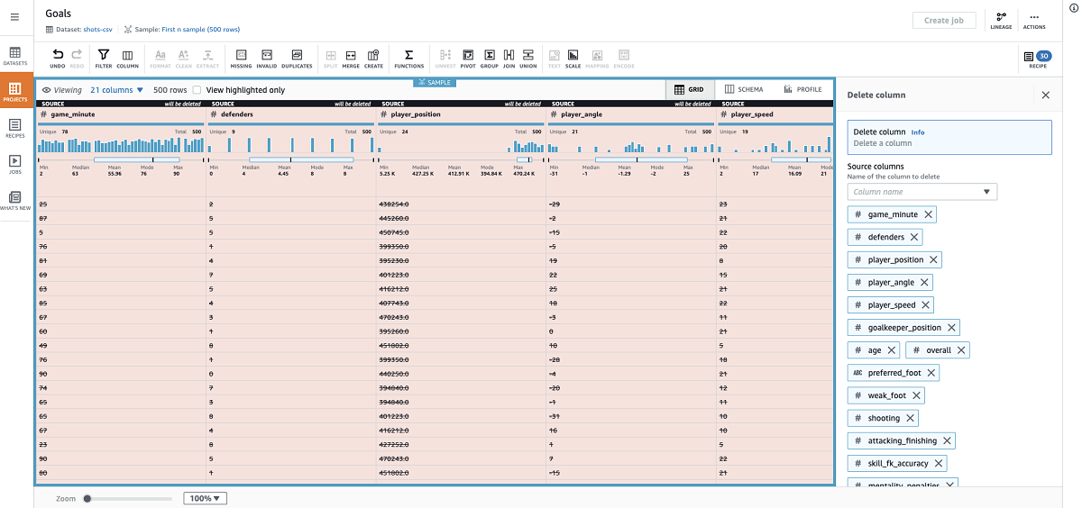
17. Now that I have the normalized columns, I can delete all their source columns.

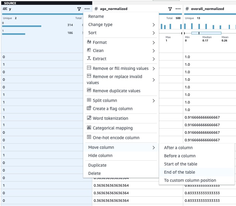
18. Lastly, I move the result column all the way to the end because this is my output column (what I intend to predict).

19. Now we have a complete recipe and it’s time to run a job to apply the steps on the full dataset and generate an output file to use to train our model.

Training the model

When the job is finished, I retrieve the output from my Amazon Simple Storage Service (Amazon S3) bucket. This rich dataset is now ready to be fed into a model. Logistic regression or Support Vector Machines (SVM) could be good candidates for our dataset. You could use Amazon SageMaker to train a model and generate a probability of scoring per event. The following screenshot shows a basic logistic regression model created using scikit-learn.

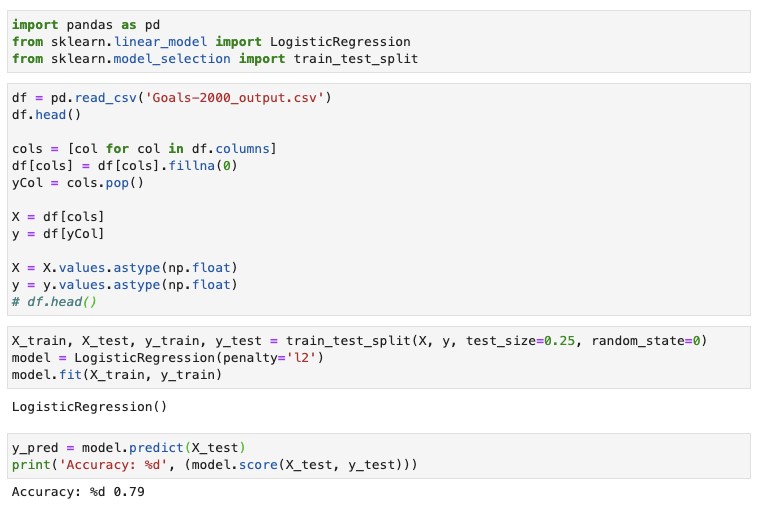
We see an approximately 80% probability that this model correctly predicts a scoring opportunity. You may get even higher accuracy using SVM. Feel free to try those or edit one of your data preparation steps and see how it affects your model accuracy.

Conclusion

In this post, we started with some raw fictionalized data of soccer shots and players. We framed the problem based on our domain knowledge and the data available. We used DataBrew to rapidly and visually connect the dots and forge the original datasets into an enriched form that could be used to train an ML model.

I encourage you to apply the same methodology to a problem domain that interests you and see how DataBrew can speed up your workflow.

---

About the Author

Arash Rowshan is a Software Engineer at Amazon Web Services. He’s passionate about big data and applications of ML. Most recently he was part of the team that launched AWS Glue DataBrew. Any time he’s not at his desk, he’s likely playing soccer somewhere. You can follow him on Twitter @OSO_Arash.