All posts by Arun Shanmugam

Beyond JSON blobs: Implementing the VARIANT data type in Apache Iceberg V3

Post Syndicated from Arun Shanmugam original https://aws.amazon.com/blogs/big-data/beyond-json-blobs-implementing-the-variant-data-type-in-apache-iceberg-v3/

Apache Iceberg V3 introduces the VARIANT data type. VARIANT provides data engineers with a high-performance, native solution for managing semi-structured data within the data lake. Consider a massive fleet of IoT sensors: street-level temperature probes, air quality monitors, and vehicle telemetry. Each device emits data in unique JSON structures that constantly evolve with firmware updates.

Historically, engineers were forced to store these payloads as STRING blobs. This legacy approach mandates expensive CPU-intensive parsing at runtime and inflates storage costs with redundant raw text. VARIANT solves these inefficiencies by employing a shredded, binary-encoded format. This allows query engines to skip irrelevant data and access specific nested fields with columnar speed, effectively bridging the gap between the flexibility of JSON and the performance of a structured schema.

VARIANT is stored in Parquet as a three-part group: binary metadata (type and dictionary info), a binary value (the full variant for fallback), and a typed_value group where individual JSON fields are shredded into separate Parquet columns. When you query a specific field, Spark prunes the typed_value group to include only the requested sub-columns. It always retains metadata and the value fallback, so it avoids reading the entire document. This approach delivers two concrete benefits:

  • Reduced query processing time: Queries access only the fields they need without deserializing entire JSON documents. This reduces the amount of data scanned and the time spent on deserialization.
  • Lower storage footprint: Binary encoding compresses more efficiently than raw text, reducing storage costs.

Fields inside the JSON become individually accessible columns under the hood. A query that needs one value out of a deeply nested document no longer must read and deserialize the entire thing. You maintain schema flexibility while gaining the performance characteristics of structured columnar storage.

This post is part 1 of a two-part series. We walk through the basics: creating an Iceberg V3 table with a VARIANT column, inserting semi-structured data, and querying it with variant_get(). In Part 2, we scale to millions of rows and benchmark VARIANT against traditional string storage. We measure the difference in query performance and storage footprint.

Solution overview

This walkthrough demonstrates an end-to-end workflow for working with semi-structured data using the VARIANT data type in Apache Iceberg V3 on Amazon EMR Serverless. Raw JSON payloads are ingested and converted to binary VARIANT format using parse_json(). The data is stored in an Iceberg V3 table where the engine shreds the structure into columnar Parquet sub-columns. You can then query the data efficiently using variant_get() to extract specific fields without deserializing the entire document. AWS Glue Data Catalog manages the table metadata. Amazon Simple Storage Service (Amazon S3) provides the underlying storage.

Note: Check the Apache Iceberg documentation for the latest information on specification status and engine compatibility. Additionally, Fine-Grained Access Control (FGAC) through AWS Lake Formation is not currently supported for the VARIANT data type.

How VARIANT works

When you insert a JSON document into a VARIANT column, Spark converts it from a JSON string into the Variant binary format. During writes, the engine can shred the structure. It extracts individual fields and stores them as native Parquet-typed sub-columns within the VARIANT column’s typed_value group. Fields that are not shredded remain in the binary value column as a fallback. This is conceptually similar to how a columnar table stores each column independently. The difference is that the sub-columns live within a single VARIANT column, and the engine handles the shredding schema automatically.

At query time, when you ask for a specific field using variant_get(), Spark reads only the sub-column that contains that field. It does not need to load or parse the rest of the document. For workloads that repeatedly query a handful of fields out of large, complex JSON payloads, this can significantly reduce the amount of data scanned. It also reduces the time spent deserializing it.

The variant_get() function uses JSON path syntax to navigate the structure. You can extract scalar values with an explicit type (optional), access nested objects, and reach into arrays by index. The function signature is the following.

variant_get(column, '$.path.to.field', 'type')

Where column is the VARIANT column name, the second argument is a JSON path expression, and the optional third argument specifies the expected return type (such as 'string', 'int', or 'double'). When the type argument is omitted, the function returns a VARIANT value that preserves the original encoding.

Running Iceberg V3 on Amazon EMR Serverless

Amazon EMR Serverless 8.0 ships with Apache Spark 4.0.1, which includes native support for Iceberg V3 and the VARIANT data type. You do not need to install additional libraries or configure custom JARs. Amazon EMR Serverless manages the compute infrastructure and scales resources up and down based on workload demand. You can focus on the data rather than the cluster.

While this post uses Amazon EMR Serverless, Iceberg V3 VARIANT support is also available on Amazon EMR on EC2 and Amazon EMR on EKS. You can choose the deployment model that fits your environment.

Getting started

The following walkthrough creates an Iceberg V3 table with a VARIANT column, inserts a set of IoT sensor events, and runs queries to extract fields from the semi-structured payload. Each step includes the code you need to run it on Amazon EMR Serverless.

Prerequisites

Before you begin, verify you have the following:

  • An AWS account with permissions to create Amazon EMR Serverless applications and access Amazon Simple Storage Service (Amazon S3).
  • An Amazon S3 bucket for storing Iceberg table data and scripts.
  • AWS Glue Data Catalog configured for metadata management.
  • An IAM execution role with permissions for Amazon EMR Serverless, Amazon S3, AWS Glue, and Amazon CloudWatch Logs.
  • AWS Command Line Interface (AWS CLI) installed and configured.Note: Running this solution in your AWS account might incur charges for Amazon EMR Serverless, Amazon S3, and AWS Glue. Refer to the respective pricing pages for cost details.

Step 1: Initialize a Spark session with Iceberg V3

Start by creating a Spark session configured to use the Iceberg catalog backed by AWS Glue. The key settings are the Iceberg Spark extensions and the AWS Glue catalog implementation. Replace <YOUR_S3_BUCKET> with your bucket name.

from pyspark.sql import SparkSession
from pyspark.sql.functions import col, parse_json

spark = SparkSession.builder \
    .appName("IcebergV3VariantDemo") \
    .config("spark.sql.extensions",
            "org.apache.iceberg.spark.extensions.IcebergSparkSessionExtensions") \
    .config("spark.sql.catalog.glue_catalog",
            "org.apache.iceberg.spark.SparkCatalog") \
    .config("spark.sql.catalog.glue_catalog.warehouse",
            "s3://<YOUR_S3_BUCKET>/warehouse/") \
    .config("spark.sql.catalog.glue_catalog.catalog-impl",
            "org.apache.iceberg.aws.glue.GlueCatalog") \
    .config("spark.sql.catalog.glue_catalog.io-impl",
            "org.apache.iceberg.aws.s3.S3FileIO") \
    .getOrCreate()

When running on Amazon EMR Serverless, some Spark configurations might be set at the application or job level. The configuration shown here is included in the script for completeness. Depending on your Amazon EMR Serverless application settings, you might not need to specify all these properties in the script.

Step 2: Create an Iceberg V3 table with a VARIANT column

Create a namespace and table. The format version must be set to 3 for VARIANT data type support. The following table models IoT sensor events with a few standard columns and a VARIANT column for the semi-structured payload.

spark.sql("CREATE NAMESPACE IF NOT EXISTS glue_catalog.iceberg_v3_demo")

spark.sql("""
CREATE TABLE IF NOT EXISTS glue_catalog.iceberg_v3_demo.sensor_events (
    event_id STRING,
    device_id STRING,
    event_timestamp TIMESTAMP,
    event_data VARIANT
)
USING iceberg
TBLPROPERTIES (
    'format-version' = '3'
)
""")

The event_data column is declared as VARIANT. Iceberg stores it in Parquet as a binary-encoded VARIANT structure (metadata, value, and optional shredded sub-columns) rather than as a plain text string.

Step 3: Insert semi-structured data

To insert JSON data into a VARIANT column, use the parse_json() function. This converts a JSON string into the binary VARIANT format at write time. The following example creates a small DataFrame of IoT events and appends them to the table.

import json
from pyspark.sql.functions import current_timestamp
from pyspark.sql.types import StructType, StructField, StringType

# Sample IoT events with nested JSON payloads
events = [
    ("evt_001", "sensor_001", json.dumps({
        "device": {"manufacturer": "SensorTech", "model": "ST-200",
                   "firmware_version": "3.1.4"},
        "sensors": {"temperature": 22.5, "humidity": 61.3,
                    "air_quality": {"pm25": 12.4, "co2": 415}},
        "network": {"connection": "WiFi", "latency_ms": 42},
        "alerts": [{"severity": "low", "message": "Calibration due"}]
    })),
    ("evt_002", "sensor_002", json.dumps({
        "device": {"manufacturer": "IoTCorp", "model": "IC-500",
                   "firmware_version": "2.8.1"},
        "sensors": {"temperature": 34.1, "humidity": 78.9,
                    "air_quality": {"pm25": 142.7, "co2": 1850}},
        "network": {"connection": "LTE", "latency_ms": 210},
        "alerts": [{"severity": "critical",
                    "message": "Temperature threshold exceeded"},
                   {"severity": "high",
                    "message": "Poor air quality detected"}]
    })),
    ("evt_003", "sensor_003", json.dumps({
        "device": {"manufacturer": "SmartDevices", "model": "SD-100",
                   "firmware_version": "1.5.9"},
        "sensors": {"temperature": 18.7, "humidity": 45.2,
                    "air_quality": {"pm25": 8.1, "co2": 390}},
        "network": {"connection": "Ethernet", "latency_ms": 5},
        "alerts": []
    })),
]

schema = StructType([
    StructField("event_id", StringType(), False),
    StructField("device_id", StringType(), False),
    StructField("event_data", StringType(), False),
])

df = spark.createDataFrame(events, schema)
df = df.withColumn("event_timestamp", current_timestamp())

# Convert JSON string to VARIANT using parse_json
df = df.withColumn("event_data", parse_json(col("event_data")))

df.writeTo("glue_catalog.iceberg_v3_demo.sensor_events").append()
print("Data inserted successfully.")

The parse_json() call is the key step. It takes the raw JSON string and encodes it into the binary VARIANT format before writing to the Iceberg table.

Step 4: Query VARIANT data with variant_get()

Once the data is in the table, you can extract individual fields from the VARIANT column using variant_get(). The following queries demonstrate three common patterns: simple field extraction, deep nested access with filtering, and array element access.

The following queries are shown as raw SQL for readability. To run them in your PySpark script, wrap each query in a spark.sql() call. For example: spark.sql("SELECT ...").show().

Query 1: Simple field extraction

Extract top-level sensor readings from the payload.

SELECT
    event_id,
    device_id,
    variant_get(event_data, '$.sensors.temperature', 'double') AS temperature,
    variant_get(event_data, '$.sensors.humidity', 'double') AS humidity
FROM glue_catalog.iceberg_v3_demo.sensor_events

This query reads only the temperature and humidity sub-columns from the VARIANT data. It does not parse or load the rest of the JSON document.

Query 2: Deep nested access with filtering

Reach into nested objects and filter on a value buried inside the structure.

SELECT
    device_id,
    variant_get(event_data, '$.sensors.air_quality.pm25', 'double') AS pm25,
    variant_get(event_data, '$.sensors.air_quality.co2', 'int') AS co2_level,
    variant_get(event_data, '$.device.manufacturer', 'string') AS manufacturer
FROM glue_catalog.iceberg_v3_demo.sensor_events
WHERE variant_get(event_data, '$.sensors.air_quality.pm25', 'double') > 100.0

The WHERE clause filters directly on a nested VARIANT field. Spark evaluates the predicate against the shredded sub-column without deserializing the full payload.

Query 3: Array element access

Access elements inside a JSON array stored within the VARIANT column.

SELECT
    event_id,
    device_id,
    variant_get(event_data, '$.alerts[0].severity', 'string') AS first_alert_severity,
    variant_get(event_data, '$.alerts[0].message', 'string') AS first_alert_message
FROM glue_catalog.iceberg_v3_demo.sensor_events
WHERE variant_get(event_data, '$.alerts[0].severity', 'string') = 'critical'

Array indexing uses standard bracket notation in the JSON path. This query finds events where the first alert has critical severity and returns the alert details.
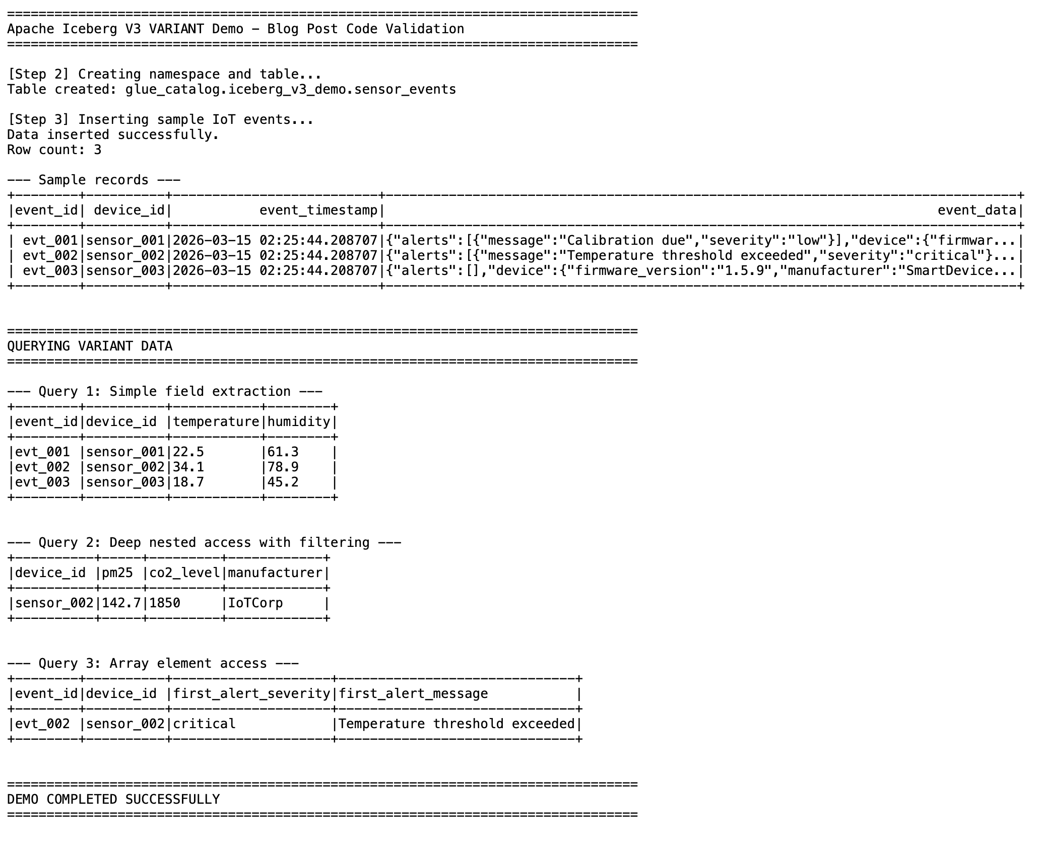
Query results showing simple field extraction, nested access with filtering, and array element access from the VARIANT column

Figure 1: Query results showing simple field extraction, nested access with filtering, and array element access from the VARIANT column.

Submitting the job to Amazon EMR Serverless

To run this on Amazon EMR Serverless, save the preceding code as a single PySpark script (for example, iceberg_v3_variant_demo.py), upload it to Amazon S3, and submit it as a job. Replace the placeholder values with your own.

Before submitting the job, make sure you have created an Amazon EMR Serverless application. For instructions, see Getting started with Amazon EMR Serverless in the Amazon EMR documentation.

# Upload script to S3
aws s3 cp iceberg_v3_variant_demo.py \
    s3://<YOUR_S3_BUCKET>/scripts/ \
    --region <REGION>

# Submit the job
aws emr-serverless start-job-run \
    --application-id <APPLICATION_ID> \
    --execution-role-arn arn:aws:iam::<ACCOUNT_ID>:role/EMRServerlessExecutionRole \
    --job-driver '{
        "sparkSubmit": {
            "entryPoint": "s3://<YOUR_S3_BUCKET>/scripts/iceberg_v3_variant_demo.py"
        }
    }' \
    --configuration-overrides '{
        "monitoringConfiguration": {
            "cloudWatchLoggingConfiguration": {
                "enabled": true,
                "logGroupName": "/aws/emr-serverless/applications/<APPLICATION_ID>"
            }
        }
    }' \
    --region <REGION>

Use cases

VARIANT fits naturally into workloads where the data is semi-structured and the schema is not fully known in advance. Some use cases include the following:

  • IoT and sensor data: Device fleets produce telemetry in varying JSON formats that evolve with firmware updates. VARIANT stores these payloads without requiring a fixed schema, and queries can extract specific readings without scanning the entire document.
  • Clickstream analytics: User behavior events on websites and mobile apps carry different attributes depending on the action. Page views, clicks, form submissions, and purchases each have their own structure. VARIANT accommodates these data types in a single column.
  • Log analytics: Application logs, infrastructure metrics, and audit trails often arrive as unstructured or loosely structured JSON. VARIANT lets you ingest them as is and query specific fields on demand, without defining a schema up front.

Clean up

To avoid ongoing charges, delete the resources you created:

  • Drop the Iceberg table and namespace using Spark SQL.
    spark.sql("DROP TABLE IF EXISTS glue_catalog.iceberg_v3_demo.sensor_events")
    spark.sql("DROP NAMESPACE IF EXISTS glue_catalog.iceberg_v3_demo")

  • Stop and delete the Amazon EMR Serverless application.
    aws emr-serverless delete-application --application-id <APPLICATION_ID> --region <REGION>

  • Delete the S3 objects and bucket used for table data, scripts, and logs.
    aws s3 rm s3://<YOUR_S3_BUCKET>/warehouse/ --recursive
    aws s3 rm s3://<YOUR_S3_BUCKET>/scripts/ --recursive

Conclusion

Apache Iceberg V3’s VARIANT type provides an efficient way to store and query semi-structured data in your data lake. Columnar storage and shredding reduce storage costs, and direct field access through variant_get() removes the need to parse JSON strings at query time. On Amazon EMR Serverless, you get this capability without managing infrastructure.

In Part 2 of this series, we scale to millions of rows and benchmark VARIANT against traditional string storage. We measure query performance and storage footprint under realistic workloads.

To learn more about Apache Iceberg on AWS, see Apache Iceberg on AWS prescriptive guidance. For more information about Amazon EMR Serverless, see the Amazon EMR Serverless documentation.
About the authors

Arun Shanmugam

Arun Shanmugam

Arun is a Senior Analytics Solutions Architect at AWS, with a focus on building modern data architecture. He has been successfully delivering scalable data analytics solutions for customers across diverse industries. Outside of work, Arun is an avid outdoor enthusiast who actively engages in CrossFit, road biking, and cricket.

Suthan Phillips

Suthan Phillips

Suthan is a Senior Analytics Architect at AWS, where he helps customers design and optimize scalable, high-performance data solutions that drive business insights. He combines architectural guidance on system design and scalability with best practices to provide efficient, secure implementation across data processing and experience layers. Outside of work, Suthan enjoys swimming, hiking, and exploring the Pacific Northwest.

Ron Ortloff

Ron Ortloff

Ron Ortloff is a Principal Product Manager at AWS, where he focuses on Apache Iceberg, S3 Tables, and open data lakehouse solutions. He has over 15 years of experience building and leading data platform initiatives, including launching Azure Synapse Analytics at Microsoft and leading Iceberg and data lake strategy at Snowflake. When he’s not building data platforms, Ron can be found cheering on his favorite football and hockey teams.

Xiaoxuan Li

Xiaoxuan Li

Xiaoxuan is a Software Development Engineer at AWS, working on the performance and scalability of Apache Iceberg in large-scale data lakehouse systems. Her interests span query optimization, storage-efficient architectures, and distributed data processing. Outside of work, she explores AI systems for creative storytelling and tooling for writers and content creators.

Unlock the power of Apache Iceberg v3 deletion vectors on Amazon EMR

Post Syndicated from Arun Shanmugam original https://aws.amazon.com/blogs/big-data/unlock-the-power-of-apache-iceberg-v3-deletion-vectors-on-amazon-emr/

As modern data architectures expand, Apache Iceberg has become a widely popular open table format, providing ACID transactions, time travel, and schema evolution. In table format v2, Iceberg introduced merge-on-read, improving delete and update handling through positional delete files. These files improve write performance but can slow down reads when not compacted, since Iceberg must merge them during query execution to return the latest snapshot. Iceberg v3 enhances merge performance during reads by replacing positional delete files with deletion vectors for handling row-level deletes in Merge-on-Read (MoR) tables. This change deprecates the use of positional delete files in v3, which marked specific row positions as deleted, in favor of the more efficient deletion vectors.

In this post, we compare and evaluate the performance of the new binary deletion vectors in Iceberg v3 with respect to traditional position delete files of Iceberg v2 using Amazon EMR version 7.10.0 with Apache Spark 3.5.5. We provide insights into the practical impacts of these advanced row-level delete mechanisms on data management efficiency and performance.

Understanding binary deletion vectors and Puffin files

Binary deletion vectors stored in Puffin files use compressed bitmaps to efficiently represent which rows have been deleted within a data file. In contrast, previous Iceberg versions (v2) relied on positional delete files—Parquet files that enumerated rows to delete by file and position. This older approach resulted in many small delete files, which placed a heavy burden on query engines due to numerous file reads and costly in-memory conversions. Puffin files reduce this overhead by compactly encoding deletions, improving query performance and resource utilization.

Iceberg v3 improves this in the following aspects:

  • Reduced I/O – Fewer small delete files lower metadata overhead by introducing deletion vectors—compressed bitmaps that efficiently represent deleted rows. These vectors are stored persistently in Puffin files, a compact binary format optimized for low-latency access.
  • Query performance – Bitmap-based deletion vectors enable faster scan filtering by allowing multiple vectors to be stored in a single Puffin file. This reduces metadata and file count overhead while preserving file-level granularity for efficient reads. The design supports continuous merging of deletion vectors, promoting ongoing compaction that maintains stable query performance and reduces fragmentation over time. It removes the trade-off between partition-level and file-level delete granularity seen in v2, enabling consistently fast reads even in heavy-update scenarios.
  • Storage efficiency – Iceberg v3 uses a compressed binary format instead of verbose Parquet positioning. Engines maintain a single deletion vector per data file at write time, enabling better compaction and consistent query performance.

Solution overview

To explore the performance characteristics of delete operations in Iceberg v2 and v3, we use PySpark to run our comparison tests focusing on delete operation runtime and delete file size. This implementation helps us effectively benchmark and compare the deletion mechanisms between Iceberg v2’s position-delete files using Parquet and v3’s newer Puffin-based deletion vectors.

Our solution demonstrates how to configure Spark with the AWS Glue Data Catalog and Iceberg, create tables, and run delete operations programmatically. We first create Iceberg tables with format versions 2 and 3, insert 10,000 rows, then perform delete operations on a range of record IDs. We also perform table compaction and then measure delete operation runtime and size and count of associated delete files.

In Iceberg v3, deleting rows introduces binary deletion vectors stored in Puffin files (compact binary sidecar files). These allow more efficient query planning and faster read performance by consolidating deletes and avoiding large numbers of small files.

For this test, the Spark job was submitted by SSH’ing into the EMR cluster and using spark-submit directly from the shell, with the required Iceberg JAR file being referenced directly from the Amazon Simple Storage Service (Amazon S3) bucket in the submission command. When running the job, make sure you provide your S3 bucket name. See the following code:

spark-submit --jars s3://< S3-BUCKET-NAME >/iceberg/jars/iceberg-spark-runtime-3.5_2.12-1.9.2.jar v3_deletion_vector_test.py

Prerequisites

To follow along with this post, you must have the following prerequisites:

  • Amazon EMR on Amazon EC2 with version 7.10.0 integrated with the Glue Data Catalog, which includes Spark 3.5.5.
  • The Iceberg 1.9.2 JAR file from the official Iceberg documentation, which includes important deletion vector improvements such as v2 to v3 rewrites and dangling deletion vector detection. Optionally, you can use the default Iceberg 1.8.1-amzn-0 bundled with Amazon EMR 7.10 if these Iceberg 1.9.x improvements are not required.
  • An S3 bucket to store Iceberg data.
  • An AWS Identity and Access management (IAM) role for Amazon EMR configured with the necessary permissions.

The upcoming Amazon EMR 7.11 will ship with Iceberg 1.9.1-amzn-1, which includes deletion vector improvements such as v2 to v3 rewrites and dangling deletion vector detection. This means you no longer need to manually download or upload the Iceberg JAR file, because it will be included and managed natively by Amazon EMR.

Code walkthrough

The following PySpark script demonstrates how to create, write, compact, and delete records in Iceberg tables with two different format versions (v2 and v3) using the Glue Data Catalog as the metastore. The main goal is to compare both write and read performance, along with storage characteristics (delete file format and size) between Iceberg format versions 2 and 3.

The code performs the following functions:

  • Creates a SparkSession configured to use Iceberg with Glue Data Catalog integration.
  • Creates a synthetic dataset simulating user records:
    • Uses a fixed random seed (42) to provide consistent data generation
    • Creates identical datasets for both v2 and v3 tables for fair comparison
  • Defines the function test_read_performance(table_name) to perform the following actions:
    • Measure full table scan performance
    • Measure filtered read performance (with WHERE clause)
    • Track record counts for both operations
  • Defines the function test_iceberg_table(version, test_df) to perform the following actions:
    • Create or use an Iceberg table for the specified format version
    • Append data to the Iceberg table
    • Trigger Iceberg’s data compaction using a system procedure
    • Delete rows with IDs between 1000–1099
    • Collect statistics about inserted data files and delete-related files
    • Measure and record read performance metrics
    • Track operation timing for inserts, deletes, and reads
  • Defines a function to print a comprehensive comparative report including the following information:
    • Delete operation performance
    • Read performance (both full table and filtered)
    • Delete file characteristics (formats, counts, sizes)
    • Performance improvements as percentages
    • Storage efficiency metrics
  • Orchestrate the main execution flow:
    • Create a single dataset to ensure identical data for both versions
    • Clean up existing tables for fresh testing
    • Run tests for Iceberg format version 2 and version 3
    • Output a detailed comparison report
    • Handle exceptions and shut down the Spark session

See the following code:

from pyspark.sql import SparkSession
from pyspark.sql.types import StructType, StructField, IntegerType, StringType
from pyspark.sql import functions as F
import time
import random
import logging
from pyspark.sql.utils import AnalysisException
# Logging
logging.basicConfig(level=logging.INFO, format='%(message)s')
logger = logging.getLogger(__name__)
# Constants
ROWS_COUNT = 10000
DELETE_RANGE_START = 1000
DELETE_RANGE_END = 1099
SAMPLE_NAMES = ["Alice", "Bob", "Charlie", "Diana",
                "Eve", "Frank", "Grace", "Henry", "Ivy", "Jack"]
# Spark Session
spark = (
    SparkSession.builder
    .appName("IcebergWithGlueCatalog")
    .config("spark.sql.extensions", "org.apache.iceberg.spark.extensions.IcebergSparkSessionExtensions")
    .config("spark.sql.catalog.glue_catalog", "org.apache.iceberg.spark.SparkCatalog")
    .config("spark.sql.catalog.glue_catalog.catalog-impl", "org.apache.iceberg.aws.glue.GlueCatalog")
    .config("spark.sql.catalog.glue_catalog.warehouse", "s3://<S3-BUCKET-NAME>/blog/glue/")
    .config("spark.sql.catalog.glue_catalog.io-impl", "org.apache.iceberg.aws.s3.S3FileIO")
    .getOrCreate()
)
spark.sql("CREATE DATABASE IF NOT EXISTS glue_catalog.blog")
def create_dataset(num_rows=ROWS_COUNT):
    # Set a fixed seed for reproducibility
    random.seed(42)
    
    data = [(i,
             random.choice(SAMPLE_NAMES) + str(i),
             random.randint(18, 80))
            for i in range(1, num_rows + 1)]
    schema = StructType([
        StructField("id", IntegerType(), False),
        StructField("name", StringType(), True),
        StructField("age", IntegerType(), True)
    ])
    df = spark.createDataFrame(data, schema)
    df = df.withColumn("created_at", F.current_timestamp())
    return df
def test_read_performance(table_name):
    """Test read performance of the table"""
    start_time = time.time()
    count = spark.sql(f"SELECT COUNT(*) FROM glue_catalog.blog.{table_name}").collect()[0][0]
    read_time = time.time() - start_time
    
    # Test filtered read performance
    start_time = time.time()
    filtered_count = spark.sql(f"""
        SELECT COUNT(*) 
        FROM glue_catalog.blog.{table_name} 
        WHERE age > 30
    """).collect()[0][0]
    filtered_read_time = time.time() - start_time
    
    return read_time, filtered_read_time, count, filtered_count
def test_iceberg_table(version, test_df):
    try:
        table_name = f"iceberg_table_v{version}"
        logger.info(f"\n=== TESTING ICEBERG V{version} ===")
        spark.sql(f"""
            CREATE TABLE IF NOT EXISTS glue_catalog.blog.{table_name} (
                id int,
                name string,
                age int,
                created_at timestamp
            ) USING iceberg
            TBLPROPERTIES (
                'format-version'='{version}',
                'write.delete.mode'='merge-on-read'
            )
        """)
        start_time = time.time()
        test_df.writeTo(f"glue_catalog.blog.{table_name}").append()
        insert_time = time.time() - start_time
        logger.info("Compaction...")
        spark.sql(
            f"CALL glue_catalog.system.rewrite_data_files('glue_catalog.blog.{table_name}')")
        start_time = time.time()
        spark.sql(f"""
            DELETE FROM glue_catalog.blog.{table_name}
            WHERE id BETWEEN {DELETE_RANGE_START} AND {DELETE_RANGE_END}
        """)
        delete_time = time.time() - start_time
        files_df = spark.sql(
            f"SELECT COUNT(*) as data_files FROM glue_catalog.blog.{table_name}.files")
        delete_files_df = spark.sql(f"""
            SELECT COUNT(*) as delete_files,
                   file_format,
                   SUM(file_size_in_bytes) as total_size
            FROM glue_catalog.blog.{table_name}.delete_files
            GROUP BY file_format
        """)
        data_files = files_df.collect()[0]['data_files']
        delete_stats = delete_files_df.collect()
        # Add read performance testing
        logger.info("\nTesting read performance...")
        read_time, filtered_read_time, total_count, filtered_count = test_read_performance(table_name)
        
        logger.info(f"Insert time: {insert_time:.3f}s")
        logger.info(f"Delete time: {delete_time:.3f}s")
        logger.info(f"Full table read time: {read_time:.3f}s")
        logger.info(f"Filtered read time: {filtered_read_time:.3f}s")
        logger.info(f"Data files: {data_files}")
        logger.info(f"Total records: {total_count}")
        logger.info(f"Filtered records: {filtered_count}")
        if len(delete_stats) > 0:
            stats = delete_stats[0]
            logger.info(f"Delete files: {stats.delete_files}")
            logger.info(f"Delete format: {stats.file_format}")
            logger.info(f"Delete files size: {stats.total_size} bytes")
            return delete_time, stats.total_size, stats.file_format, read_time, filtered_read_time
        else:
            logger.info("No delete files found")
            return delete_time, 0, "N/A", read_time, filtered_read_time
    except AnalysisException as e:
        logger.error(f"SQL Error: {str(e)}")
        raise
    except Exception as e:
        logger.error(f"Error: {str(e)}")
        raise
def print_comparison_results(v2_results, v3_results):
    v2_delete_time, v2_size, v2_format, v2_read_time, v2_filtered_read_time = v2_results
    v3_delete_time, v3_size, v3_format, v3_read_time, v3_filtered_read_time = v3_results
    logger.info("\n=== PERFORMANCE COMPARISON ===")
    logger.info(f"v2 delete time: {v2_delete_time:.3f}s")
    logger.info(f"v3 delete time: {v3_delete_time:.3f}s")
    if v2_delete_time > 0:
        improvement = ((v2_delete_time - v3_delete_time) / v2_delete_time) * 100
        logger.info(f"v3 Delete performance improvement: {improvement:.1f}%")
    logger.info("\n=== READ PERFORMANCE COMPARISON ===")
    logger.info(f"v2 full table read time: {v2_read_time:.3f}s")
    logger.info(f"v3 full table read time: {v3_read_time:.3f}s")
    logger.info(f"v2 filtered read time: {v2_filtered_read_time:.3f}s")
    logger.info(f"v3 filtered read time: {v3_filtered_read_time:.3f}s")
    
    if v2_read_time > 0:
        read_improvement = ((v2_read_time - v3_read_time) / v2_read_time) * 100
        logger.info(f"v3 Read performance improvement: {read_improvement:.1f}%")
    
    if v2_filtered_read_time > 0:
        filtered_improvement = ((v2_filtered_read_time - v3_filtered_read_time) / v2_filtered_read_time) * 100
        logger.info(f"v3 Filtered read performance improvement: {filtered_improvement:.1f}%")
    logger.info("\n=== DELETE FILE COMPARISON ===")
    logger.info(f"v2 delete format: {v2_format}")
    logger.info(f"v2 delete size: {v2_size} bytes")
    logger.info(f"v3 delete format: {v3_format}")
    logger.info(f"v3 delete size: {v3_size} bytes")
    if v2_size > 0:
        size_reduction = ((v2_size - v3_size) / v2_size) * 100
        logger.info(f"v3 size reduction: {size_reduction:.1f}%")
# Main
try:
    # Create dataset once and reuse for both versions
    test_dataset = create_dataset()
    
    # Drop existing tables if they exist
    spark.sql("DROP TABLE IF EXISTS glue_catalog.blog.iceberg_table_v2")
    spark.sql("DROP TABLE IF EXISTS glue_catalog.blog.iceberg_table_v3")
    
    # Test both versions with the same dataset
    v2_results = test_iceberg_table(2, test_dataset)
    v3_results = test_iceberg_table(3, test_dataset)
    print_comparison_results(v2_results, v3_results)
finally:
    spark.stop()

Results summary

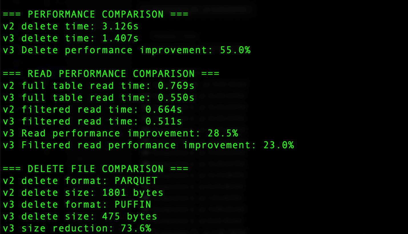
The output generated by the code includes the results summary section that shows several key comparisons, as shown in the following screenshot. For delete operations, Iceberg v3 uses the Puffin file format compared to Parquet in v2, resulting in significant improvements. The delete operation time decreased from 3.126 seconds in v2 to 1.407 seconds in v3, achieving a 55.0% performance improvement. Additionally, the delete file size was reduced from 1801 bytes using Parquet in v2 to 475 bytes using Puffin in v3, representing a 73.6% reduction in storage overhead. Read operations also saw notable improvements, with full table reads 28.5% faster and filtered reads 23% faster in v3. These improvements demonstrate the efficiency gains from v3’s implementation of binary deletion vectors through the Puffin format.

style=

The actual measured performance and storage improvements depend on workload and environment and might differ from the preceding example.

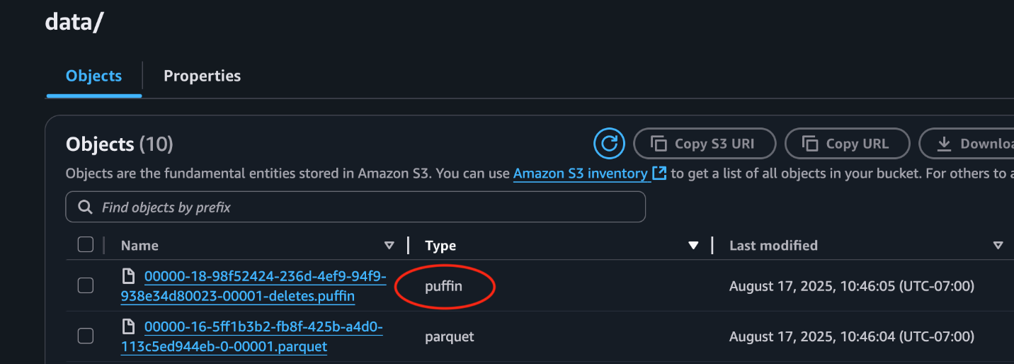
This following screenshot from the S3 bucket demonstrates a Puffin delete file stored alongside data files.

style=

Clean up

After you finish your tests, it’s important to clean up your environment to avoid unnecessary costs:

  1. Drop the test tables you created to remove associated data from your S3 bucket and prevent ongoing storage charges.
  2. Delete any temporary data left in the S3 bucket used for Iceberg data.
  3. Delete the EMR cluster to stop billing for running compute resources.

Cleaning up resources promptly helps maintain cost-efficiency and resource hygiene in your AWS environment.

Considerations

Iceberg features are introduced through a phased process: first in the specification, then in the core library, and finally in engine implementations. Deletion vector support is currently available in the specification and core library, with Spark being the only supported engine. We validated this capability on Amazon EMR 7.10 with Spark 3.5.5.

Conclusion

Iceberg v3 introduces a significant advancement in managing row-level deletes for merge-on-read operations through binary deletion vectors stored in compact Puffin files. Our performance tests, conducted with Iceberg 1.9.2 on Amazon EMR 7.10.0 and EMR Spark 3.5.5, show clear improvements in both delete operation speed and read performance, along with a considerable reduction in delete file storage compared to Iceberg v2’s positional delete Parquet files. For more information about deletion vectors, refer to Iceberg v3 deletion vectors.


About the authors

Arun Shanmugam

Arun Shanmugam

Arun is a Senior Analytics Solutions Architect at AWS, with a focus on building modern data architecture. He has been successfully delivering scalable data analytics solutions for customers across diverse industries. Outside of work, Arun is an avid outdoor enthusiast who actively engages in CrossFit, road biking, and cricket.

Suthan Phillips

Suthan Phillips

Suthan is a Senior Analytics Architect at AWS, where he helps customers design and optimize scalable, high-performance data solutions that drive business insights. He combines architectural guidance on system design and scalability with best practices to provide efficient, secure implementation across data processing and experience layers. Outside of work, Suthan enjoys swimming, hiking, and exploring the Pacific Northwest.

Kinshuk Paharae

Kinshuk Paharae

Kinshuk is head of product for data processing, leading product teams for AWS Glue, Amazon EMR, and Amazon Athena. He has been with AWS for over 5 years.

Linda OConnor

Linda OConnor

Linda is a Seasoned Go-To-Market Leader with close to three decades of experience driving growth strategies in the data and analytics space. At AWS, she currently leads pan analytics initiatives including lakehouse architectures, helping customers transform their existing landscapes through non-disruptive innovation. She previously served as Global Vice President at a German software company for 25 years, where she spearheaded Data Warehousing and Big Data portfolios, orchestrating successful product launches and driving global market expansion.