Amazon Web Services (AWS) provides many mechanisms to optimize the price performance of workloads running on Amazon Elastic Compute Cloud (Amazon EC2), and the selection of the optimal infrastructure to run on can be one of the most impactful levers. When we started building the AWS Graviton processor, our goal was to optimize AWS Graviton features and capabilities to deliver a processor that provides the best price performance across a broad array of cloud workloads running on Amazon EC2. That goal continues to be our guiding principle, and today customers who adopt AWS Graviton-based EC2 instances see up to 40% better price performance on their cloud workloads when compared to equivalent non-Graviton EC2 instances. The price performance improvement is the result of both the performance improvement and the lower price in using AWS Graviton-based instances.
Price performance blends the cost of infrastructure with the amount of work you can achieve with infrastructure usage. After talking to many AWS Graviton customers, we’ve learned that the cost savings go beyond the lower AWS Graviton-based instances price. Many AWS Graviton customers told us that the performance increase from AWS Graviton allows them to consume fewer computing hours than comparable non-Graviton instances for equivalent workload throughput. In turn, this leads to further cost reduction.
The following are some of examples from our customers:
Pinterest achieved 47% cost savings and 38% savings on compute resources while reducing carbon emissions by 62% for its web API workload.
SAP powers its SAP HANA Cloud with AWS Graviton to enhance its price performance by 35% while lowering carbon impact by 45%.
Sprinklr improved their machine learning (ML) inference workloads’ throughput by up to 20% while reducing costs by up to 25%.
To help organizations capture similar benefits, we’ve enhanced the AWS Graviton Savings Dashboard (GSD) with new features that account for both pricing and performance improvements. In the following section we explore these new capabilities and how they can help optimize your infrastructure costs.
Understanding performance-driven cost optimization in the GSD
The GSD helps organizations identify ideal workloads for AWS Graviton migration through automated resource matching and data-driven visualizations. You can learn the GSD details and setup in this AWS compute post.
Although the dashboard has traditionally focused on calculating direct cost savings from the AWS Graviton pricing advantages, we’ve observed that customers often experience more benefits when their applications perform more efficiently on AWS Graviton processors, leading to decreased compute resource usage. To better reflect these real-world scenarios, we’ve enhanced the dashboard with new features highlighting Normalized Instance Hours (NIH) analysis capabilities so that you can model potential savings based on both pricing benefits and compute hour reductions. Although this tool helps estimate potential savings, actual performance improvements can only be determined by testing your specific workloads on AWS Graviton instances. Performance is always workload and use case specific, so we encourage you to test your AWS Graviton-based workloads using the Optimization and Performance Runbook to help you determine the actual possible NIH percent reduction.
Key dashboard components
This section outlines the following three key dashboard components: NIH reduction analysis, enhanced cost analysis visualizations, and detailed savings analysis.
NIH reduction analysis
The dashboard now features a new slider that lets you model potential cost savings by inputting the percentage reduction in NIH. Many organizations have found it challenging to calculate their total possible savings since the benefits come from two sources: the lower instance pricing of AWS Graviton and the reduced compute hours.
You can use the slider to model different cost scenarios by adjusting a theoretical NIH reduction between 0% and 40%. You can use this slider to input NIH reductions validated through your workload testing, model the combined impact of both pricing benefits and reduced compute hours, and explore different scenarios to help prioritize which workloads to test first.
Figure 1: NIH slider location
Assume that your testing shows that your workload runs just as effectively with 15% fewer normalized instance hours on AWS Graviton. You can now plug that exact number into the slider to see your modeled savings combining both pricing differences and compute hour reductions. Although we’ve heard success stories of significant reductions from customers, we recommend starting your initial estimate with a conservative 10% baseline and adjusting based on your own testing results.
Enhanced cost analysis visualizations
The dashboard presents key visualizations that demonstrate the direct relationship between NIH reduction and cost savings. First, you see the Potential Graviton Base Savings from pricing differences alone. In the following diagram, we can observe an example of $61.54K of cost savings from migrating to equivalent AWS Graviton instances. Next, the Estimated Additional Savings Due to Performance in the same diagram shows $42.40K in savings if your performance testing confirms a 15% NIH reduction in your workload. Finally, the dashboard sums these two values into the Total Potential Graviton Savings of $103.94K. The Total Potential Graviton Savings helps visualize how both pricing benefits and any validated compute hour reductions could contribute to your overall savings.
Figure 2: Visualization with relationship between NIH reduction and cost savings
The Amortized Cost Breakdown and Normalized Instance Hrs Breakdown charts in the following figure show 6-month historical trends, helping you spot patterns such as seasonal spikes or high-usage periods. These patterns can help you identify where even small efficiency improvements might yield significant savings, for example, workloads with consistently high usage or predictable peak periods that would be good candidates for testing.
Figure 3: Amortized Cost, NIH, and Total Potential Savings Breakdown charts
Detailed savings analysis
Building on our commitment to help customers optimize cloud costs, we’ve enhanced the Potential Graviton Savings Details table with two columns focused on performance-based savings modeling. The Estimated Additional Savings Due to Performance column shows the modeled savings based on your chosen NIH reduction percentage, while Total Potential Graviton Savings combines this with the base pricing benefits.
As you examine your current instance family, you can observe both baseline AWS Graviton savings and these added saving opportunities clearly laid out in a comprehensive breakdown. The analysis presents your total savings potential in both dollar amounts and percentages. This allows you to build a compelling business case for migration. Although this detailed breakdown provides valuable planning insights, remember that actual savings may vary depending on your specific workload patterns, implementation approaches, and operational considerations.
Conclusion
The Graviton Savings Dashboard (GSD) serves as a powerful analytics tool that streamlines your journey to cost-effective cloud computing. The GSD provides clear visualizations and interactive features to help you understand and maximize potential savings when migrating to AWS Graviton-based instances. To further explore the new features, navigate to the GSD interactive demo, where you can model an example of potential savings using the NIH reduction slider and detailed cost breakdowns.
Ready to explore how AWS Graviton can transform your infrastructure costs? Visit the GSD page to deploy or update your GSD dashboard. Access implementation guides, such as the CFM Technical Implementation Playbook (CFM TIPs), and start optimizing your cloud spend today with the enhanced capabilities of the GSD.
Over 85,000 AWS customers have discovered the benefits of AWS Graviton, with many completing their adoptions in just hours. We have created this resource guide so that you can accelerate your AWS Graviton adoption with minimal effort and enjoy significant price performance benefits.
“What I always tell customers is one week, one application, one engineer, and see what you can do. They always are pleasantly surprised by how much progress they can make. If you’re out there and you haven’t yet moved to AWS Graviton, what are you waiting for? Let’s make it happen!”
Dave Brown, VP, AWS Compute & ML Services
Important note about performance testing The GSD does not attempt to estimate the potential NIH percent reduction or your workload’s performance when transitioned to AWS Graviton. You can use it to perform what-if analysis of your potential savings for a projected NIH percent reduction. In the absence of this variable, GSD only considers the price delta between instance types and misses an important contributor to the overall savings potential of AWS Graviton from the performance upside. Compute performance is always workload and use case specific, so we encourage you to test your AWS Graviton-based workloads using the Optimization and Performance Runbook to help you determine the actual possible NIH percent reduction.
As modern data architectures expand, Apache Iceberg has become a widely popular open table format, providing ACID transactions, time travel, and schema evolution. In table format v2, Iceberg introduced merge-on-read, improving delete and update handling through positional delete files. These files improve write performance but can slow down reads when not compacted, since Iceberg must merge them during query execution to return the latest snapshot. Iceberg v3 enhances merge performance during reads by replacing positional delete files with deletion vectors for handling row-level deletes in Merge-on-Read (MoR) tables. This change deprecates the use of positional delete files in v3, which marked specific row positions as deleted, in favor of the more efficient deletion vectors.
In this post, we compare and evaluate the performance of the new binary deletion vectors in Iceberg v3 with respect to traditional position delete files of Iceberg v2 using Amazon EMR version 7.10.0 with Apache Spark 3.5.5. We provide insights into the practical impacts of these advanced row-level delete mechanisms on data management efficiency and performance.
Understanding binary deletion vectors and Puffin files
Binary deletion vectors stored in Puffin files use compressed bitmaps to efficiently represent which rows have been deleted within a data file. In contrast, previous Iceberg versions (v2) relied on positional delete files—Parquet files that enumerated rows to delete by file and position. This older approach resulted in many small delete files, which placed a heavy burden on query engines due to numerous file reads and costly in-memory conversions. Puffin files reduce this overhead by compactly encoding deletions, improving query performance and resource utilization.
Iceberg v3 improves this in the following aspects:
Reduced I/O – Fewer small delete files lower metadata overhead by introducing deletion vectors—compressed bitmaps that efficiently represent deleted rows. These vectors are stored persistently in Puffin files, a compact binary format optimized for low-latency access.
Query performance – Bitmap-based deletion vectors enable faster scan filtering by allowing multiple vectors to be stored in a single Puffin file. This reduces metadata and file count overhead while preserving file-level granularity for efficient reads. The design supports continuous merging of deletion vectors, promoting ongoing compaction that maintains stable query performance and reduces fragmentation over time. It removes the trade-off between partition-level and file-level delete granularity seen in v2, enabling consistently fast reads even in heavy-update scenarios.
Storage efficiency – Iceberg v3 uses a compressed binary format instead of verbose Parquet positioning. Engines maintain a single deletion vector per data file at write time, enabling better compaction and consistent query performance.
Solution overview
To explore the performance characteristics of delete operations in Iceberg v2 and v3, we use PySpark to run our comparison tests focusing on delete operation runtime and delete file size. This implementation helps us effectively benchmark and compare the deletion mechanisms between Iceberg v2’s position-delete files using Parquet and v3’s newer Puffin-based deletion vectors.
Our solution demonstrates how to configure Spark with the AWS Glue Data Catalog and Iceberg, create tables, and run delete operations programmatically. We first create Iceberg tables with format versions 2 and 3, insert 10,000 rows, then perform delete operations on a range of record IDs. We also perform table compaction and then measure delete operation runtime and size and count of associated delete files.
In Iceberg v3, deleting rows introduces binary deletion vectors stored in Puffin files (compact binary sidecar files). These allow more efficient query planning and faster read performance by consolidating deletes and avoiding large numbers of small files.
For this test, the Spark job was submitted by SSH’ing into the EMR cluster and using spark-submit directly from the shell, with the required Iceberg JAR file being referenced directly from the Amazon Simple Storage Service (Amazon S3) bucket in the submission command. When running the job, make sure you provide your S3 bucket name. See the following code:
The upcoming Amazon EMR 7.11 will ship with Iceberg 1.9.1-amzn-1, which includes deletion vector improvements such as v2 to v3 rewrites and dangling deletion vector detection. This means you no longer need to manually download or upload the Iceberg JAR file, because it will be included and managed natively by Amazon EMR.
Code walkthrough
The following PySpark script demonstrates how to create, write, compact, and delete records in Iceberg tables with two different format versions (v2 and v3) using the Glue Data Catalog as the metastore. The main goal is to compare both write and read performance, along with storage characteristics (delete file format and size) between Iceberg format versions 2 and 3.
The code performs the following functions:
Creates a SparkSession configured to use Iceberg with Glue Data Catalog integration.
Creates a synthetic dataset simulating user records:
Uses a fixed random seed (42) to provide consistent data generation
Creates identical datasets for both v2 and v3 tables for fair comparison
Defines the function test_read_performance(table_name) to perform the following actions:
Measure full table scan performance
Measure filtered read performance (with WHERE clause)
Track record counts for both operations
Defines the function test_iceberg_table(version, test_df) to perform the following actions:
Create or use an Iceberg table for the specified format version
Append data to the Iceberg table
Trigger Iceberg’s data compaction using a system procedure
Delete rows with IDs between 1000–1099
Collect statistics about inserted data files and delete-related files
Measure and record read performance metrics
Track operation timing for inserts, deletes, and reads
Defines a function to print a comprehensive comparative report including the following information:
Create a single dataset to ensure identical data for both versions
Clean up existing tables for fresh testing
Run tests for Iceberg format version 2 and version 3
Output a detailed comparison report
Handle exceptions and shut down the Spark session
See the following code:
from pyspark.sql import SparkSession
from pyspark.sql.types import StructType, StructField, IntegerType, StringType
from pyspark.sql import functions as F
import time
import random
import logging
from pyspark.sql.utils import AnalysisException
# Logging
logging.basicConfig(level=logging.INFO, format='%(message)s')
logger = logging.getLogger(__name__)
# Constants
ROWS_COUNT = 10000
DELETE_RANGE_START = 1000
DELETE_RANGE_END = 1099
SAMPLE_NAMES = ["Alice", "Bob", "Charlie", "Diana",
                "Eve", "Frank", "Grace", "Henry", "Ivy", "Jack"]
# Spark Session
spark = (
    SparkSession.builder
    .appName("IcebergWithGlueCatalog")
    .config("spark.sql.extensions", "org.apache.iceberg.spark.extensions.IcebergSparkSessionExtensions")
    .config("spark.sql.catalog.glue_catalog", "org.apache.iceberg.spark.SparkCatalog")
    .config("spark.sql.catalog.glue_catalog.catalog-impl", "org.apache.iceberg.aws.glue.GlueCatalog")
    .config("spark.sql.catalog.glue_catalog.warehouse", "s3://<S3-BUCKET-NAME>/blog/glue/")
    .config("spark.sql.catalog.glue_catalog.io-impl", "org.apache.iceberg.aws.s3.S3FileIO")
    .getOrCreate()
)
spark.sql("CREATE DATABASE IF NOT EXISTS glue_catalog.blog")
def create_dataset(num_rows=ROWS_COUNT):
    # Set a fixed seed for reproducibility
    random.seed(42)

    data = [(i,
             random.choice(SAMPLE_NAMES) + str(i),
             random.randint(18, 80))
            for i in range(1, num_rows + 1)]
    schema = StructType([
        StructField("id", IntegerType(), False),
        StructField("name", StringType(), True),
        StructField("age", IntegerType(), True)
    ])
    df = spark.createDataFrame(data, schema)
    df = df.withColumn("created_at", F.current_timestamp())
    return df
def test_read_performance(table_name):
    """Test read performance of the table"""
    start_time = time.time()
    count = spark.sql(f"SELECT COUNT(*) FROM glue_catalog.blog.{table_name}").collect()[0][0]
    read_time = time.time() - start_time

    # Test filtered read performance
    start_time = time.time()
    filtered_count = spark.sql(f"""
        SELECT COUNT(*)
        FROM glue_catalog.blog.{table_name}
        WHERE age > 30
    """).collect()[0][0]
    filtered_read_time = time.time() - start_time

    return read_time, filtered_read_time, count, filtered_count
def test_iceberg_table(version, test_df):
    try:
        table_name = f"iceberg_table_v{version}"
        logger.info(f"\n=== TESTING ICEBERG V{version} ===")
        spark.sql(f"""
            CREATE TABLE IF NOT EXISTS glue_catalog.blog.{table_name} (
                id int,
                name string,
                age int,
                created_at timestamp
            ) USING iceberg
            TBLPROPERTIES (
                'format-version'='{version}',
                'write.delete.mode'='merge-on-read'
            )
        """)
        start_time = time.time()
        test_df.writeTo(f"glue_catalog.blog.{table_name}").append()
        insert_time = time.time() - start_time
        logger.info("Compaction...")
        spark.sql(
            f"CALL glue_catalog.system.rewrite_data_files('glue_catalog.blog.{table_name}')")
        start_time = time.time()
        spark.sql(f"""
            DELETE FROM glue_catalog.blog.{table_name}
            WHERE id BETWEEN {DELETE_RANGE_START} AND {DELETE_RANGE_END}
        """)
        delete_time = time.time() - start_time
        files_df = spark.sql(
            f"SELECT COUNT(*) as data_files FROM glue_catalog.blog.{table_name}.files")
        delete_files_df = spark.sql(f"""
            SELECT COUNT(*) as delete_files,
                   file_format,
                   SUM(file_size_in_bytes) as total_size
            FROM glue_catalog.blog.{table_name}.delete_files
            GROUP BY file_format
        """)
        data_files = files_df.collect()[0]['data_files']
        delete_stats = delete_files_df.collect()
        # Add read performance testing
        logger.info("\nTesting read performance...")
        read_time, filtered_read_time, total_count, filtered_count = test_read_performance(table_name)

        logger.info(f"Insert time: {insert_time:.3f}s")
        logger.info(f"Delete time: {delete_time:.3f}s")
        logger.info(f"Full table read time: {read_time:.3f}s")
        logger.info(f"Filtered read time: {filtered_read_time:.3f}s")
        logger.info(f"Data files: {data_files}")
        logger.info(f"Total records: {total_count}")
        logger.info(f"Filtered records: {filtered_count}")
        if len(delete_stats) > 0:
            stats = delete_stats[0]
            logger.info(f"Delete files: {stats.delete_files}")
            logger.info(f"Delete format: {stats.file_format}")
            logger.info(f"Delete files size: {stats.total_size} bytes")
            return delete_time, stats.total_size, stats.file_format, read_time, filtered_read_time
        else:
            logger.info("No delete files found")
            return delete_time, 0, "N/A", read_time, filtered_read_time
    except AnalysisException as e:
        logger.error(f"SQL Error: {str(e)}")
        raise
    except Exception as e:
        logger.error(f"Error: {str(e)}")
        raise
def print_comparison_results(v2_results, v3_results):
    v2_delete_time, v2_size, v2_format, v2_read_time, v2_filtered_read_time = v2_results
    v3_delete_time, v3_size, v3_format, v3_read_time, v3_filtered_read_time = v3_results
    logger.info("\n=== PERFORMANCE COMPARISON ===")
    logger.info(f"v2 delete time: {v2_delete_time:.3f}s")
    logger.info(f"v3 delete time: {v3_delete_time:.3f}s")
    if v2_delete_time > 0:
        improvement = ((v2_delete_time - v3_delete_time) / v2_delete_time) * 100
        logger.info(f"v3 Delete performance improvement: {improvement:.1f}%")
    logger.info("\n=== READ PERFORMANCE COMPARISON ===")
    logger.info(f"v2 full table read time: {v2_read_time:.3f}s")
    logger.info(f"v3 full table read time: {v3_read_time:.3f}s")
    logger.info(f"v2 filtered read time: {v2_filtered_read_time:.3f}s")
    logger.info(f"v3 filtered read time: {v3_filtered_read_time:.3f}s")

    if v2_read_time > 0:
        read_improvement = ((v2_read_time - v3_read_time) / v2_read_time) * 100
        logger.info(f"v3 Read performance improvement: {read_improvement:.1f}%")

    if v2_filtered_read_time > 0:
        filtered_improvement = ((v2_filtered_read_time - v3_filtered_read_time) / v2_filtered_read_time) * 100
        logger.info(f"v3 Filtered read performance improvement: {filtered_improvement:.1f}%")
    logger.info("\n=== DELETE FILE COMPARISON ===")
    logger.info(f"v2 delete format: {v2_format}")
    logger.info(f"v2 delete size: {v2_size} bytes")
    logger.info(f"v3 delete format: {v3_format}")
    logger.info(f"v3 delete size: {v3_size} bytes")
    if v2_size > 0:
        size_reduction = ((v2_size - v3_size) / v2_size) * 100
        logger.info(f"v3 size reduction: {size_reduction:.1f}%")
# Main
try:
    # Create dataset once and reuse for both versions
    test_dataset = create_dataset()

    # Drop existing tables if they exist
    spark.sql("DROP TABLE IF EXISTS glue_catalog.blog.iceberg_table_v2")
    spark.sql("DROP TABLE IF EXISTS glue_catalog.blog.iceberg_table_v3")

    # Test both versions with the same dataset
    v2_results = test_iceberg_table(2, test_dataset)
    v3_results = test_iceberg_table(3, test_dataset)
    print_comparison_results(v2_results, v3_results)
finally:
    spark.stop()
Results summary
The output generated by the code includes the results summary section that shows several key comparisons, as shown in the following screenshot. For delete operations, Iceberg v3 uses the Puffin file format compared to Parquet in v2, resulting in significant improvements. The delete operation time decreased from 3.126 seconds in v2 to 1.407 seconds in v3, achieving a 55.0% performance improvement. Additionally, the delete file size was reduced from 1801 bytes using Parquet in v2 to 475 bytes using Puffin in v3, representing a 73.6% reduction in storage overhead. Read operations also saw notable improvements, with full table reads 28.5% faster and filtered reads 23% faster in v3. These improvements demonstrate the efficiency gains from v3’s implementation of binary deletion vectors through the Puffin format.
The actual measured performance and storage improvements depend on workload and environment and might differ from the preceding example.
This following screenshot from the S3 bucket demonstrates a Puffin delete file stored alongside data files.
Clean up
After you finish your tests, it’s important to clean up your environment to avoid unnecessary costs:
Drop the test tables you created to remove associated data from your S3 bucket and prevent ongoing storage charges.
Delete any temporary data left in the S3 bucket used for Iceberg data.
Delete the EMR cluster to stop billing for running compute resources.
Cleaning up resources promptly helps maintain cost-efficiency and resource hygiene in your AWS environment.
Considerations
Iceberg features are introduced through a phased process: first in the specification, then in the core library, and finally in engine implementations. Deletion vector support is currently available in the specification and core library, with Spark being the only supported engine. We validated this capability on Amazon EMR 7.10 with Spark 3.5.5.
Conclusion
Iceberg v3 introduces a significant advancement in managing row-level deletes for merge-on-read operations through binary deletion vectors stored in compact Puffin files. Our performance tests, conducted with Iceberg 1.9.2 on Amazon EMR 7.10.0 and EMR Spark 3.5.5, show clear improvements in both delete operation speed and read performance, along with a considerable reduction in delete file storage compared to Iceberg v2’s positional delete Parquet files. For more information about deletion vectors, refer to Iceberg v3 deletion vectors.
This post is written by Goeksel Sarikaya, Senior Delivery Consultant at AWS, and Milosz Stawarski, Senior Software Architect at Stellantis.
Software licensing is a critical aspect of many organizations’ operations, with various models available to suit different needs. Two common types are named user licenses, which are assigned to specific individuals, and floating licenses, which can be shared among a pool of users. Some independent software vendors (ISVs) offer both options, whereas others might have limitations, particularly in cloud environments.
In this post, we explore a unique scenario where an ISV, unable to provide a floating license option for cloud usage, worked with Stellantis to develop an alternative solution. This approach, implemented with the ISV’s permission, treats named user licenses as if they were floating, automatically assigning and removing them based on the state of user workbench instances.
This solution is not intended to circumvent licensing terms or reduce costs at the expense of ISVs. Rather, it’s a collaborative approach to address specific customer needs when traditional floating licenses aren’t available. We will demonstrate how the solution uses serverless AWS services like Amazon EventBridge, AWS Lambda, Amazon DynamoDB, and AWS Systems Manager, keeping in mind that any similar implementation should only be pursued with explicit permission from the software vendor.
Overview of Stellantis
Stellantis N.V., born from the merger of FCA and PSA Group, leads the change towards software defined vehicles (SDV). As part of this transformation, AWS and Stellantis created the Virtual Engineering Workbench (VEW), a modular framework to develop, integrate, and test vehicle software in the cloud, ultimately connecting their vehicles to the cloud.
The VEW provides predefined environments tailored to specific use cases. These environments come fully equipped with the tools, integrated development environments (IDEs), and licensing necessary for developers to jumpstart their projects.
As the number of developers and projects grew, Stellantis faced a challenge in managing the limited number of named user licenses for their software tools. The manual process of assigning and revoking licenses became increasingly time-consuming and inefficient, potentially hindering the agility and productivity of their development teams.
Stellantis and AWS tackled this challenge head-on by collaborating on an innovative, dynamic license management solution using AWS serverless services. This solution transforms the traditional named user license model into a more flexible floating license system, automatically assigning and revoking licenses based on the state of user workbench instances. The licenses and solution discussed in this post pertain solely to the use of standalone software tools such as those used in automotive domains. These do not involve sharing of user data or content when licenses are reused.
Before we dive into the detailed workflow of the solution, let’s examine the high-level architecture. The following diagram illustrates how various AWS services work together to create this efficient license management system.
Architecture
This architecture uses key AWS services such as EventBridge, Lambda, DynamoDB, and Systems Manager to create a scalable, serverless solution that significantly reduces administrative overhead and optimizes license utilization.
In the following sections, we explore each component of this architecture in detail, explaining how they interact to provide a seamless license management experience for Stellantis’ VEW.
In workbench accounts (user accounts)
The design is serverless and based on an event-driven approach. The workflow in the user accounts is as follows:
Workbench instances are Amazon Elastic Compute Cloud (Amazon EC2). Their start and stop automatically sends AWS events.
An EventBridge rule invokes a Lambda function when such an event occurs. This function checks the tags on the EC2 instance to distinguish workbenches from other EC2 instances. Two tags are important for identifying workbench instances: vew:workbench:ownerId and vew:workbench:type.
The Lambda function creates a custom event with the following data: user-id, workbench-type, workbench-state, and instance-id, and sends this event to the default event bus.
An EventBridge rule forwards the custom event to a custom event bus in the license server account.
In license server account
The following steps take place in the license server account:
An EventBridge rule invokes a Lambda
This function interacts with a DynamoDB table that stores a mapping of licensed products to users. The function does the following:
Deduces the licensed products present in the workbench from the workbench type.
For each licensed product, it verifies if the combination of product and user is already present in the DynamoDB
If the workbench is starting:
If the combination is already present, it increases the count of workbenches in the table for this item by 1.
If the combination is not present, it creates a new item in the table (product, user-id, workbench-count, timestamp).
If the workbench is stopping, it decreases the count of workbenches in the table for this item by 1. If the count becomes 0, the item is deleted.
Any update to the DynamoDB table triggers another Lambda
If the change in the table is a creation of a new entry or deletion of an entry, this function writes the current timestamp to a Systems Manager parameter in both cases. This is so that if no changes are detected in the database, we don’t unnecessarily run the xLC (License Client for related product) caller function.
Another Lambda function is invoked every minute. It compares the timestamp written in the Systems Manager parameter indicating a DynamoDB item creation or deletion with the last time the function called the xLC CLI to assign users to a license.
If the DynamoDB timestamp is earlier, the function stops. If the DynamoDB timestamp is later, the function queries the table for obtaining the user-id for each product.
To maintain a comprehensive record of license assignment operations, you can enable data plane events for DynamoDB in AWS CloudTrail.
For each licensed product, the function uses Run Command, a capability of Systems Manager, to invoke the xLC CLI API on the license server to assign named users to a license for a product. The function provides the list of users assigned to the product to the API. This updates the named user list on the license server—the list is completely overwritten, which includes adding new user IDs and removing ones that are no longer needed.
Benefits and key features
The solution offers the following benefits:
Automated license assignment and removal – Users are automatically assigned licenses when their workbench instances start, and licenses are returned to the pool when instances stop, providing efficient license utilization.
Scalable and serverless architecture – The solution is built on serverless AWS services, allowing it to scale seamlessly as the number of users and workbench instances grows, without the need for provisioning or managing servers.
Centralized license management – The license server account acts as a central hub for managing licenses across multiple workbench accounts, simplifying administration and providing a unified view of license usage.
Reduced administrative overhead – By automating the license assignment and removal process, the solution can significantly reduce the administrative burden associated with manual license management.
Optimized license utilization – Licenses are assigned only when needed and returned to the pool when no longer required, maximizing license availability and minimizing idle licenses.
Monitoring and metrics – The solution provides monitoring capabilities and license usage metrics, enabling better visibility and informed decision-making regarding license procurement and allocation.
Conclusion
By implementing this serverless solution, it is possible to transform a manual named user license management systems to an automated floating license system for software tools. The event-driven architecture and serverless components provide efficient and scalable license assignment and removal based on the workbench instance state.
This solution has streamlined the license management process, reducing administrative overhead and optimizing license utilization. It is now possible to provision software tools more efficiently, improving productivity and resource allocation across the organization. Additionally, the centralized license management and monitoring capabilities provide better visibility and control over license usage, enabling informed decision-making and cost optimization.
Overall, this AWS based floating license solution has empowered organizations to use software tools more effectively, while minimizing the operational burden associated with license management. For more serverless learning resources, visit Serverless Land.
Many organizations build and operate enterprise-wide data mesh architectures using the AWS GlueData Catalog and AWS Lake Formation for their Amazon Simple Storage Service (Amazon S3) based data lakes. Now, with Amazon SageMaker Lakehouse, these organizations can unify their data analytics and AI/ML workflows while maintaining secure cross-account access without data replication. By centralizing access to a single copy of data and using the secure fine-grained permissions of Lake Formation, enterprises can accelerate their analytics initiatives while reducing operational complexity across business units.
SageMaker Lakehouse organizes data using logical containers called catalogs, enabling teams to seamlessly query and analyze data across their entire ecosystem—from S3 data lakes to Amazon Redshift warehouses—using familiar Apache Iceberg compatible tools. Organizations can either mount their existing data warehouse to the lakehouse or create new catalogs using Amazon Redshift managed storage. Built-in zero-ETL connectors reduce data silos by integrating various data sources, enabling unified analytics across teams. This seamless integration particularly benefits existing AWS customers who already use the Data Catalog and Lake Formation, because they can immediately take advantage of SageMaker Lakehouse capabilities.
AWS Glue is a serverless service that makes data integration simpler, faster, and cheaper. We launched AWS Glue 5.0 with upgraded Apache Spark 3.5.4 and Python 3.11. AWS Glue 5.0 adds support for SageMaker Lakehouse to unify your data across S3 data lakes and Redshift data warehouses.
In our previous blog post, we demonstrated the process of creating tables in both the Amazon Redshift managed catalog and Amazon Redshift federated catalog within a single AWS account. In this post, we show you how to share a Redshift table and Amazon S3 based Iceberg table from the account that owns the data to another account that consumes the data. In the recipient account, we run a join query on the shared data lake and data warehouse tables using Spark in AWS Glue 5.0. We walk you through the complete cross-account setup and provide the Spark configuration in a Python notebook.
Solution overview
To demonstrate the functionality of SageMaker Lakehouse multi-catalog tables using AWS Glue 5.0 Spark, let’s assume the retail company Example Retail Corp launches a campaign to understand their market and drive growth by country of operation. Their infrastructure consists of a Redshift data warehouse for structured data and an S3 data lake for structured and semi-structured data. The marketing team realizes that customer data is spread across those two systems and wants to use the support of their data engineering and analysts to analyze and provide insights. As a company, they prefer unified governance for managing data access while enabling a secure sharing mechanism for business and engineering teams.
Let’s see how they can achieve the goal using SageMaker Lakehouse. The solution is represented in the following diagram.
The setup could be extended to enterprise data meshes where a data producer account will own the Redshift clusters, catalog the tables in a central governance account, and share with any number of consumer accounts from the central account. Multiple consumer accounts could analyze the shared Redshift tables using the SageMaker Lakehouse integrated analytics engines.
The solution also works for cross-Region table access. You would create a resource link for the catalog tables in an AWS Region where you want to run your analyses and create dashboards. For cross-Region resource link setup, refer to Setting up cross-Region table access.
Prerequisites
To implement this solution, you need the following prerequisites:
Two sample datasets, orders and returns, in CSV format. This is Example Retail Corp’s data on their customer purchase and return trends. Their marketing team has collected these data in a Redshift table and Amazon S3 from various systems. The instructions to create these tables are provided in the appendix at the end of this post. After completing the steps in the appendix, you should have customerdb.returnstbl_iceberg in your default catalog and ordersdb.orderstbl in your Redshift Serverless application default namespace.
An IAM role, Glue-execution-role, in the consumer account, with the following policies:
AWS managed policies AWSGlueServiceRole and AmazonRedshiftDataFullAccess.
Create a new in-line policy with the following permissions and attach it:
For the producer account setup, you can either use your IAM administrator role added as Lake Formation administrator or use a Lake Formation administrator role with permissions added as discussed in the prerequisites. For illustration purposes, we use the IAM admin role Admin added as Lake Formation administrator.
Configure your catalog
Complete the following steps to set up your catalog:
After the registration is initiated, you will see the invite from Amazon Redshift on the Lake Formation console.
Select the pending catalog invitation and choose Approve and create catalog.
On the Set catalog details page, configure your catalog:
For Name, enter a name (for this post, redshiftserverless1-uswest2).
Select Access this catalog from Apache Iceberg compatible engines.
Choose the IAM role you created for the data transfer.
Choose Next.
On the Grant permissions – optional page, choose Add permissions.
Grant the Admin user Super user permissions for Catalog permissions and Grantable permissions.
Choose Add.
Verify the granted permission on the next page and choose Next.
Review the details on the Review and create page and choose Create catalog.
Wait a few seconds for the catalog to show up.
Choose Catalogs in the navigation pane and verify that the redshiftserverless1-uswest2 catalog is created.
Explore the catalog detail page to verify the ordersdb.public database.
On the database View dropdown menu, view the table and verify that the orderstbl table shows up.
As the Admin role, you can also query the orderstbl in Amazon Athena and confirm the data is available.
Grant permissions on the tables from the producer account to the consumer account
In this step, we share the Amazon Redshift federated catalog database redshiftserverless1-uswest2:ordersdb.public and table orderstbl as well as the Amazon S3 based Iceberg table returnstbl_iceberg and its database customerdb from the default catalog to the consumer account. We can’t share the entire catalog to external accounts as a catalog-level permission; we just share the database and table.
On the Lake Formation console, choose Data permissions in the navigation pane.
Choose Grant.
Under Principals, select External accounts.
Provide the consumer account ID.
Under LF-Tags or catalog resources, select Named Data Catalog resources.
For Catalogs, choose the account ID that represents the default catalog.
For Databases, choose customerdb.
Under Database permissions, select Describe under Database permissions and Grantable permissions.
Choose Grant.
Repeat these steps and grant table-level Select and Describe permissions on returnstbl_iceberg.
Repeat these steps again to grant database- and table-level permissions for the ordertbl table of the federated catalog database redshiftserverless1-uswest2/ordersdb.
The following screenshots show the configuration for database-level permissions.
The following screenshots show the configuration for table-level permissions.
Choose Data permissions in the navigation pane and verify that the consumer account has been granted database- and table-level permissions for both orderstbl from the federated catalog and returnstbl_iceberg from the default catalog.
Register the Amazon S3 location of the returnstbl_iceberg with Lake Formation.
In this step, we register the Amazon S3 based Iceberg table returnstbl_iceberg data location with Lake Formation to be managed by Lake Formation permissions. Complete the following steps:
On the Lake Formation console, choose Data lake locations in the navigation pane.
Choose Register location.
For Amazon S3 path, enter the path for your S3 bucket that you provided while creating the Iceberg table returnstbl_iceberg.
For IAM role, provide the user-defined role LakeFormationS3Registration_custom that you created as a prerequisite.
For Permission mode, select Lake Formation.
Choose Register location.
Choose Data lake locations in the navigation pane to verify the Amazon S3 registration.
With this step, the producer account setup is complete.
Steps for consumer account setup
For the consumer account setup, we use the IAM admin role Admin, added as a Lake Formation administrator.
The steps in the consumer account are quite involved. In the consumer account, a Lake Formation administrator will accept the AWS Resource Access Manager (AWS RAM) shares and create the required resource links that point to the shared catalog, database, and tables. The Lake Formation admin verifies that the shared resources are accessible by running test queries in Athena. The admin further grants permissions to the role Glue-execution-role on the resource links, database, and tables. The admin then runs a join query in AWS Glue 5.0 Spark using Glue-execution-role.
Accept and verify the shared resources
Lake Formation uses AWS RAM shares to enable cross-account sharing with Data Catalog resource policies in the AWS RAM policies. To view and verify the shared resources from producer account, complete the following steps:
Log in to the consumer AWS console and set the AWS Region to match the producer’s shared resource Region. For this post, we use us-west-2.
Open the Lake Formation console. You will see a message indicating there is a pending invite and asking you accept it on the AWS RAM console.
When the invite status changes to Accepted, choose Shared resources under Shared with me in the navigation pane.
Verify that the Redshift Serverless federated catalog redshiftserverless1-uswest2, the default catalog database customerdb, the table returnstbl_iceberg, and the producer account ID under Owner ID column display correctly.
On the Lake Formation console, under Data Catalog in the navigation pane, choose Databases.
Search by the producer account ID. You should see the customerdb and public databases. You can further select each database and choose View tables on the Actions dropdown menu and verify the table names
You will not see an AWS RAM share invite for the catalog level on the Lake Formation console, because catalog-level sharing isn’t possible. You can review the shared federated catalog and Amazon Redshift managed catalog names on the AWS RAM console, or using the AWS Command Line Interface (AWS CLI) or SDK.
Create a catalog link container and resource links
A catalog link container is a Data Catalog object that references a local or cross-account federated database-level catalog from other AWS accounts. For more details, refer to Accessing a shared federated catalog. Catalog link containers are essentially Lake Formation resource links at the catalog level that reference or point to a Redshift cluster federated catalog or Amazon Redshift managed catalog object from other accounts.
In the following steps, we create a catalog link container that points to the producer shared federated catalog redshiftserverless1-uswest2. Inside the catalog link container, we create a database. Inside the database, we create a resource link for the table that points to the shared federated catalog table <<producer account id>>:redshiftserverless1-uswest2/ordersdb.public.orderstbl.
On the Lake Formation console, under Data Catalog in the navigation pane, choose Catalogs.
Choose Create catalog.
Provide the following details for the catalog:
For Name, enter a name for the catalog (for this post, rl_link_container_ordersdb).
For Type, choose Catalog Link container.
For Source, choose Redshift.
For Target Redshift Catalog, enter the Amazon Resource Name (ARN) of the producer federated catalog (arn:aws:glue:us-west-2:<<producer account id>>:catalog/redshiftserverless1-uswest2/ordersdb).
Under Access from engines, select Access this catalog from Apache Iceberg compatible engines.
For IAM role, provide the Redshift-S3 data transfer role that you had created in the prerequisites.
Choose Next.
On the Grant permissions – optional page, choose Add permissions.
Grant the Admin user Super user permissions for Catalog permissions and Grantable permissions.
Choose Add and then choose Next.
Review the details on the Review and create page and choose Create catalog.
Wait a few seconds for the catalog to show up.
In the navigation pane, choose Catalogs.
Verify that rl_link_container_ordersdb is created.
Create a database under rl_link_container_ordersdb
Complete the following steps:
On the Lake Formation console, under Data Catalog in the navigation pane, choose Databases.
On the Choose catalog dropdown menu, choose rl_link_container_ordersdb.
Choose Create database.
Alternatively, you can choose the Create dropdown menu and then choose Database.
Provide details for the database:
For Name, enter a name (for this post, public_db).
For Catalog, choose rl_link_container_ordersdb.
Leave Location – optional as blank.
Under Default permissions for newly created tables, deselect Use only IAM access control for new tables in this database.
Choose Create database.
Choose Catalogs in the navigation pane to verify that public_db is created under rl_link_container_ordersdb.
Create a table resource link for the shared federated catalog table
A resource link to a shared federated catalog table can reside only inside the database of a catalog link container. A resource link for such tables will not work if created inside the default catalog. For more details on resource links, refer to Creating a resource link to a shared Data Catalog table.
Complete the following steps to create a table resource link:
On the Lake Formation console, under Data Catalog in the navigation pane, choose Tables.
On the Create dropdown menu, choose Resource link.
Provide details for the table resource link:
For Resource link name, enter a name (for this post, rl_orderstbl).
For Destination catalog, choose rl_link_container_ordersdb.
For Database, choose public_db.
For Shared table’s region, choose US West (Oregon).
For Shared table, choose orderstbl.
After the Shared table is selected, Shared table’s database and Shared table’s catalog ID should get automatically populated.
Choose Create.
In the navigation pane, choose Databases to verify that rl_orderstbl is created under public_db, inside rl_link_container_ordersdb.
Create a database resource link for the shared default catalog database.
Now we create a database resource link in the default catalog to query the Amazon S3 based Iceberg table shared from the producer. For details on database resource links, refer Creating a resource link to a shared Data Catalog database.
Though we are able to see the shared database in the default catalog of the consumer, a resource link is required to query from analytics engines, such as Athena, Amazon EMR, and AWS Glue. When using AWS Glue with Lake Formation tables, the resource link needs to be named identically to the source account’s resource. For additional details on using AWS Glue with Lake Formation, refer to Considerations and limitations.
Complete the following steps to create a database resource link:
On the Lake Formation console, under Data Catalog in the navigation pane, choose Databases.
On the Choose catalog dropdown menu, choose the account ID to choose the default catalog.
Search for customerdb.
You should see the shared database name customerdb with the Owner account ID as that of your producer account ID.
Select customerdb, and on the Create dropdown menu, choose Resource link.
Provide details for the resource link:
For Resource link name, enter a name (for this post, customerdb).
The rest of the fields should be already populated.
Choose Create.
In the navigation pane, choose Databases and verify that customerdb is created under the default catalog. Resource link names will show in italicized font.
Verify access as Admin using Athena
Now you can verify your access using Athena. Complete the following steps:
In the navigation pane, verify both the default catalog and federated catalog tables by previewing them.
You can also run a join query as follows. Pay attention to the three-point notation for referring to the tables from two different catalogs:
SELECT
returns_tb.market as Market,
sum(orders_tb.quantity) as Total_Quantity
FROM rl_link_container_ordersdb.public_db.rl_orderstbl as orders_tb
JOIN awsdatacatalog.customerdb.returnstbl_iceberg as returns_tb
ON orders_tb.order_id = returns_tb.order_id
GROUP BY returns_tb.market;
This verifies the new capability of SageMaker Lakehouse, which enables accessing Redshift cluster tables and Amazon S3 based Iceberg tables in the same query, across AWS accounts, through the Data Catalog, using Lake Formation permissions.
Grant permissions to Glue-execution-role
Now we will share the resources from the producer account with additional IAM principals in the consumer account. Usually, the data lake admin grants permissions to data analysts, data scientists, and data engineers in the consumer account to do their job functions, such as processing and analyzing the data.
We set up Lake Formation permissions on the catalog link container, databases, tables, and resource links to the AWS Glue job execution role Glue-execution-role that we created in the prerequisites.
Resource links allow only Describe and Drop permissions. You need to use the Grant on target configuration to provide database Describe and table Select permissions.
Complete the following steps:
On the Lake Formation console, choose Data permissions in the navigation pane.
Choose Grant.
Under Principals, select IAM users and roles.
For IAM users and roles, enter Glue-execution-role.
Under LF-Tags or catalog resources, select Named Data Catalog resources.
For Catalogs, choose rl_link_container_ordersdb and the consumer account ID, which indicates the default catalog.
Under Catalog permissions, select Describe for Catalog permissions.
Choose Grant.
Repeat these steps for the catalog rl_link_container_ordersdb:
On the Databases dropdown menu, choose public_db.
Under Database permissions, select Describe.
Choose Grant.
Repeat these steps again, but after choosing rl_link_container_ordersdb and public_db, on the Tables dropdown menu, choose rl_orderstbl.
Under Resource link permissions, select Describe.
Choose Grant.
Repeat these steps to grant additional permissions to Glue-execution-role.
For this iteration, grant Describe permissions on the default catalog databases public and customerdb.
Grant Describe permission on the resource link customerdb.
Grant Select permission on the tables returnstbl_iceberg and orderstbl.
The following screenshots show the configuration for database public and customerdb permissions.
The following screenshots show the configuration for resource link customerdb permissions.
The following screenshots show the configuration for table returnstbl_iceberg permissions.
The following screenshots show the configuration for table orderstbl permissions.
In the navigation pane, choose Data permissions and verify permissions on Glue-execution-role.
Run a PySpark job in AWS Glue 5.0
Download the PySpark script LakeHouseGlueSparkJob.py. This AWS Glue PySpark script runs Spark SQL by joining the producer shared federated orderstbl table and Amazon S3 based returns table in the consumer account to analyze the data and identify the total orders placed per market.
Replace <<consumer_account_id>> in the script with your consumer account ID. Complete the following steps to create and run an AWS Glue job:
On the AWS Glue console, in the navigation pane, choose ETL jobs.
Choose Create job, then choose Script editor.
For Engine, choose Spark.
For Options, choose Start fresh.
Choose Upload script.
Browse to the location where you downloaded and edited the script, select the script, and choose Open.
On the Job details tab, provide the following information:
For Name, enter a name (for this post, LakeHouseGlueSparkJob).
Under Basic properties, for IAM role, choose Glue-execution-role.
For Glue version, select Glue 5.0.
Under Advanced properties, for Job parameters, choose Add new parameter.
Add the parameters --datalake-formats = iceberg and --enable-lakeformation-fine-grained-access = true.
Save the job.
Choose Run to execute the AWS Glue job, and wait for the job to complete.
Review the job run details from the Output logs
Clean up
To avoid incurring costs on your AWS accounts, clean up the resources you created:
Delete the Lake Formation permissions, catalog link container, database, and tables in the consumer account.
Delete the AWS Glue job in the consumer account.
Delete the federated catalog, database, and table resources in the producer account.
Delete the Redshift Serverless namespace in the producer account.
Delete the S3 buckets you created as part of data transfer in both accounts and the Athena query results bucket in the consumer account.
Clean up the IAM roles you created for the SageMaker Lakehouse setup as part of the prerequisites.
Conclusion
In this post, we illustrated how to bring your existing Redshift tables to SageMaker Lakehouse and share them securely with external AWS accounts. We also showed how to query the shared data warehouse and data lakehouse tables in the same Spark session, from a recipient account, using Spark in AWS Glue 5.0.
We hope you find this useful to integrate your Redshift tables with an existing data mesh and access the tables using AWS Glue Spark. Test this solution in your accounts and share feedback in the comments section. Stay tuned for more updates and feel free to explore the features of SageMaker Lakehouse and AWS Glue versions.
Appendix: Table creation
Complete the following steps to create a returns table in the Amazon S3 based default catalog and an orders table in Amazon Redshift:
Download the CSV format datasets orders and returns.
Upload them to your S3 bucket under the corresponding table prefix path.
Create an Iceberg format table in the default catalog and insert data from the CSV format table:
CREATE TABLE customerdb.returnstbl_iceberg(
  `returned` string,
  `order_id` string,
  `market` string)
LOCATION 's3://<your-producer-account-bucket>/returnstbl_iceberg/'
TBLPROPERTIES (
  'table_type'='ICEBERG'
);

INSERT INTO customerdb.returnstbl_iceberg
SELECT *
FROM returnstbl_csv;

SELECT * FROM customerdb.returnstbl_iceberg LIMIT 10;
To create the orders table in the Redshift Serverless namespace, open the Query Editor v2 on the Amazon Redshift console.
Connect to the default namespace using your database admin user credentials.
Run the following commands in the SQL editor to create the database ordersdb and table orderstbl in it. Copy the data from your S3 location of the orders data to the orderstbl:
Aarthi Srinivasan is a Senior Big Data Architect with Amazon SageMaker Lakehouse. She collaborates with the service team to enhance product features, works with AWS customers and partners to architect lakehouse solutions, and establishes best practices for data governance.
Subhasis Sarkar is a Senior Data Engineer with Amazon. Subhasis thrives on solving complex technological challenges with innovative solutions. He specializes in AWS data architectures, particularly data mesh implementations using AWS CDK components.
This post demonstrates how to leverage AWS CloudFormation Lambda Hooks to enforce compliance rules at provisioning time, enabling you to evaluate and validate Lambda function configurations against custom policies before deployment. Often these policies impact the way a software should be built, restricting language versions and runtimes. A great example is applying those policies on AWS Lambda, a serverless compute service for running code without having to provision or manage servers. While AWS Lambda already manages the deprecation of runtimes, preventing you from deploying unsupported runtimes, organizations may need to provide and enforce their specific compliance rules not directly linked to the deprecation of a specific language version.
Introducing Lambda Hooks
AWS CloudFormation Lambda Hooks are a powerful feature that allows developers to evaluate CloudFormation and AWS Cloud Control API operations against custom code implemented as Lambda functions. This capability enables proactive inspection of resource configurations before provisioning, enhancing security, compliance, and operational efficiency.
Lambda Hooks provide a mechanism to intercept and evaluate various CloudFormation operations, including resource operations, stack operations, and change set operations (they can also be used with Cloud Control API, but in this post we’re focusing on CloudFormation). By activating a Lambda Hook, CloudFormation creates an entry in your account’s registry as a private Hook, allowing you to configure it for specific AWS accounts and regions. When configuring Lambda Hooks, you can specify one or more Lambda functions to be invoked during the evaluation process. These functions can be in the same AWS account and Region as the Hook, or in another Account you own, provided proper permissions are set up. The evaluation process occurs at specific points in the CloudFormation Stack lifecycle. For instance, during stack creation, update, or deletion, the configured Lambda functions are invoked to assess the proposed changes against your defined compliance rules. Based on the evaluation results, the hook can either block the operation or issue a warning, allowing the operation to proceed.
Lambda Hooks evaluate resources before they are provisioned through CloudFormation, providing a pre-emptive layer of governance. This means that non-compliant resources are caught and prevented from being deployed, rather than requiring retroactive fixes. By leveraging Lambda Hooks, organizations can automate and standardize their compliance checks across all AWS accounts and regions. This centralized approach to policy enforcement ensures consistency and reduces the overhead of managing compliance manually.
Solution Overview
The following sections demonstrate a practical use case for AWS CloudFormation Lambda Hooks, focusing on enforcing compliance rules on AWS Lambda runtimes.
Meet AnyCompany, a forward-thinking enterprise with a robust set of compliance rules governing their software development practices. Among these rules is a strict policy on the use of specific AWS Lambda runtimes.
As they continue to embrace serverless architecture, AnyCompany faces a challenge: how to prevent the deployment of Lambda functions that use non-compliant runtimes. Given their commitment to AWS CloudFormation for deploying Lambda functions, AnyCompany is keen to leverage the power of AWS CloudFormation Lambda Hooks.
We’ll explore the setup process, demonstrate the hook in action, and discuss the broader implications for maintaining compliance in a dynamic cloud environment.
Architecture
The following architecture highlights the implementation of the Lambda Hook. In this implementation, we are using AWS CloudFormation Lambda Hooks to intercept the deployment of Lambda Functions and perform the compliance checks on these resources. The Lambda Hook will interact with an AWS Lambda Function, which will perform the compliance checks. Finally, we’re using AWS Systems Manager Parameter Store to store the Configuration Parameter which contains the list of permitted Lambda Runtimes.
Figure 1: Architecture of the Solution
A Developer (or a CI/CD pipeline) deploys a CloudFormation stack containing Lambda functions.
CloudFormation invokes the respective Lambda Hook, which is configured to intercept operations on AWS Lambda Resources. We are setting this hook to “FAIL” deployment in case checks are not successful.
hook-lambda: directory containing all the code related to the CloudFormation Lambda Hook (Validation Lambda Function, and the CloudFormation template for the Solution)
sample: directory containing the code of the sample used to test the CloudFormation Lambda Hook
deploy.sh: utility script to deploy the Solution via AWS CLI
cleanup.sh: utility script to clean up the AWS CloudFormation Hook infrastructure via the AWS CLI
template.yml: AWS CloudFormation Template containing all the AWS Resources involved in the Solution
Prerequisites
You must have the following prerequisites for this solution:
An AWS account or sign up to create and activate one.
The following software installed on your development machine:
Install the AWS Command Line Interface (AWS CLI) and configure it to point to your AWS account.
Install Node.js and use a package manager such as npm.
Appropriate AWS credentials for interacting with resources in your AWS account.
Walkthrough
Creating the AWS Lambda Validation Function – Lambda Code
The CloudFormation Lambda Hook interacts with a specific Lambda (referred to as Validation Lambda throughout the rest of this post), which gets invoked during CloudFormation CREATE and UPDATE STACK operations involving Lambda Functions. The goal is to check if these Lambda functions have runtimes that comply with AnyCompany’s rules.
Below is the detailed description of the steps that the Validation Lambda function handler follows (the code is written in Typescript).
First, the Validation Lambda retrieves an environment variable containing the SSM Parameter Store parameter name which contains the compliant runtimes list. Additionally, safety checks ensure that only Lambda Resources are considered and that their Runtime property is defined.
Note that both safety checks could be skipped, since the Hook should already be configured to interact only with Lambda Resources and the Lambda’s Runtime property is always required. However, they remain in place to demonstrate how to retrieve this information from the Lambda Hook event in your handler.
const parameterName = process.env.PERMITTED_RUNTIMES_PARAM;
if (!parameterName) {
	throw new Error('Permitted Runtimes Parameter is not set');
}

const resourceProperties = event.requestData.targetModel.resourceProperties;
// Check if this is a Lambda function resource
if (event.requestData.targetType !== 'AWS::Lambda::Function') {
console.log("Resource is not a Lambda function, skipping");
	return {
		hookStatus: 'SUCCESS',
		message: 'Not a Lambda function resource, skipping validation',
		clientRequestToken: event.clientRequestToken
	}
}

// Check runtime version compliance
const runtime = resourceProperties.Runtime;
if (!runtime) {
	console.log("Runtime not defined, failing");
	return {
		hookStatus: 'FAILURE',
		errorCode: 'NonCompliant',
		message: 'Runtime is required for Lambda functions',
		clientRequestToken: event.clientRequestToken
	}
}
Then the Validation Lambda retrieves the value of the Configuration Parameter from SSM Parameter Store through a utility class called ParameterStoreService. For this post, consider that the value inside that Configuration Parameter is a list of strings, where each string contains one of the possible Lambda runtime values that you can find here (e.g. nodejs22.x,nodejs20.x,python3.11,python3.10,java17,java11,dotnet6). After retrieving the value, the Validation Lambda checks if the runtime of the Lambda Resource complies with the configured admitted runtimes. If the runtime is not compliant, you’ll receive a properly formatted response with FAILURE as hookStatus, otherwise the response will contain a SUCCESS hookStatus.
// Retrieve configuration from Parameter Store
const compliantRuntimes = await parameterStoreService.getParameterFromStore(parameterName);

// Check if Lambda runtime is permitted or not
if (!compliantRuntimes.includes(runtime)) {
console.log("Runtime " + runtime + " not compliant ");
	return {
		hookStatus: 'FAILURE',
		errorCode: 'NonCompliant',
		message: `Runtime ${runtime} is not compliant. Please use one of: ${compliantRuntimes.join(', ')}`,
		clientRequestToken: event.clientRequestToken
	}
}

return {
	hookStatus: 'SUCCESS',
	message: 'Runtime version compliance check passed',
	clientRequestToken: event.clientRequestToken
}
For more information about the possible response values of CloudFormation Lambda Hooks Lambda, have a look at this link.
Creating the validation Lambda – Lambda CloudFormation definition
The Validation Lambda function will be deployed via CloudFormation, in the same Stack with the CloudFormation Lambda Hook definition and the AWS Systems Manager Parameter Store Parameter. Here’s the fragment of the CloudFormation Template containing its definition:
Please note that the above template contains a reference to an IAM Role because the Hook requires proper permissions to call the target (Lambda Function). Here’s the IAM Role definition:
Configuring the compliant runtimes – Using Systems Manager Parameter Store
AWS Systems Manager Parameter Store is a secure, hierarchical storage service for configuration data management and secrets management, allowing users to store and retrieve data such as configurations, database strings etc. as parameter values.
In this specific example, we’ll leverage Parameter Store to store our permitted Lambda runtimes configuration. This configuration value is a StringList parameter, containing a comma-separated list of permitted runtimes. Here’s the fragment of the CloudFormation template that defines the Parameter:
Please note the usage of CloudFormation parameters for the ‘Name’ and ‘Value’ properties, allowing for dynamic input when deploying the CloudFormation template.
Deploying the Solution
To deploy the solution you can leverage the script deploy.sh in the root folder of the repository. This script will perform the following actions:
Compile and build the Validation Lambda Function
Create an Amazon S3 Bucket to store the CloudFormation Template
Upload the CloudFormation template and Lambda code to the S3 Bucket
Deploy the CloudFormation template
Testing the Lambda Hook
To test the CloudFormation Lambda Hook, deploy a simple testing CloudFormation template containing a Hello World Lambda function. First, test the Lambda configured with a permitted Lambda runtime, then modify the template to configure the Lambda with a non-compliant runtime.
Here’s the initial definition of the testing CloudFormation Template:
Please note that the Runtime value is nodejs22.x, which is currently in the list of permitted runtimes. The expectation is that the deployment of this function will succeed.
As expected, the deployment was successful. You can also see that the CloudFormation Lambda Hook has been invoked by taking a look at the CloudWatch Logs:
Figure 3: Validation Lambda Function Logs with successful validation
Now modify the original sample Template in order to set a Lambda Runtime which is not inside the list of permitted runtimes:
Deploy this template via AWS CLI with the same command used before and check the CloudFormation Console:
Figure 4: CloudFormation Console showing failed Stack deployment due to Hook intervention
As expected, the deployment was not successful. The CloudFormation Lambda Hook has been invoked, and since the Lambda Runtime was not present in the permitted runtimes list, the deployment failed.
You can also see that the hook failed In the CloudWatch Logs:
Figure 5: Validation Lambda Function Logs with validation error
Cleaning up
To clean up the resources related to the sample, you can run the script cleanup_sample.sh inside the sample folder. This script will delete the sample’s CloudFormation Template through the AWS CLI.
To cleanup the resources related to the solution described above and based on AWS CloudFormation Lambda Hook, you can leverage the script cleanup.sh in the root folder of the repository. This script will perform the following actions:
Delete the CloudFormation Stack
Empty the S3 Bucket used for the deployment of the Stack
Delete the S3 Bucket
Conclusion
In this post, you explored the implementation of CloudFormation Hooks to enforce runtime compliance in Lambda functions across your AWS infrastructure. By leveraging the Lambda hook’s capabilities, you learned how to create a preventative control that validates Lambda runtime configurations before deployment.
By activating the Lambda hook and implementing a custom Lambda function validator, you established an automated mechanism to ensure that only compliant runtimes are used within your organization’s Lambda functions during CloudFormation stack creation and updates. The solution’s integration with common development tools like AWS CLI, AWS SAM, CI/CD pipelines, and AWS CDK makes it straightforward to implement these controls within existing workflows, eliminating the need for manual runtime checks or post-deployment remediation.
The validation approach demonstrated in this post extends beyond Lambda runtimes and can be adapted to different AWS Resources supported by CloudFormation, allowing you to enforce policies on different infrastructure components offered by AWS.
While customers can perform some basic analysis within their operational or transactional databases, many still need to build custom data pipelines that use batch or streaming jobs to extract, transform, and load (ETL) data into their data warehouse for more comprehensive analysis.
Zero-ETL integration with Amazon Redshift reduces the need for custom pipelines, preserves resources for your transactional systems, and gives you access to powerful analytics. Within seconds of transactional data being written into Amazon Aurora (a fully managed modern relational database service offering performance and high availability at scale), the data is seamlessly made available in Amazon Redshift for analytics and machine learning. The data in Amazon Redshift is transactionally consistent and updates are automatically and continuously propagated.
Amazon Redshift is a fast, scalable, secure, and fully managed cloud data warehouse that makes it simple and cost-effective to analyze all your data using standard SQL and your existing ETL, business intelligence (BI), and reporting tools. Together with price-performance, Amazon Redshift offers capabilities such as serverless architecture, machine learning integration within your data warehouse and secure data sharing across the organization.
dbt helps manage data transformation by enabling teams to deploy analytics code following software engineering best practices such as modularity, continuous integration and continuous deployment (CI/CD), and embedded documentation.
dbt Cloud is a hosted service that helps data teams productionize dbt deployments. dbt Cloud offers turnkey support for job scheduling, CI/CD integrations; serving documentation, native git integrations, monitoring and alerting, and an integrated developer environment (IDE) all within a web-based UI.
In this post, we explore how to use Aurora MySQL-Compatible Edition Zero-ETL integration with Amazon Redshift and dbt Cloud to enable near real-time analytics. By using dbt Cloud for data transformation, data teams can focus on writing business rules to drive insights from their transaction data to respond effectively to critical, time sensitive events. This enables the line of business (LOB) to better understand their core business drivers so they can maximize sales, reduce costs, and further grow and optimize their business.
Solution overview
Let’s consider TICKIT, a fictional website where users buy and sell tickets online for sporting events, shows, and concerts. The transactional data from this website is loaded into an Aurora MySQL 3.05.0 (or a later version) database. The company’s business analysts want to generate metrics to identify ticket movement over time, success rates for sellers, and the best-selling events, venues, and seasons. Analysts can use this information to provide incentives to buyers and sellers who frequently use the site, to attract new users, and to drive advertising and promotions.
The Zero-ETL integration between Aurora MySQL and Amazon Redshift is set up by using a CloudFormation template to replicate raw ticket sales information to a Redshift data warehouse. After the data is in Amazon Redshift, dbt models are used to transform the raw data into key metrics such as ticket trends, seller performance, and event popularity. These insights help analysts make data-driven decisions to improve promotions and user engagement.
The following diagram illustrates the solution architecture at a high-level.
To implement this solution, complete the following steps:
This post provides a CloudFormation template as a general guide. You can review and customize it to suit your needs. Some of the resources that this stack deploys incur costs when in use.
The CloudFormation template provisions the following components
An Aurora MySQL provisioned cluster (source)
An Amazon Redshift Serverless data warehouse (target)
Zero-ETL integration between the source (Aurora MySQL) and target (Amazon Redshift Serverless)
To create your resources:
Sign in to the console.
Choose the us-east-1 AWS Region in which to create the stack.
Choose Launch Stack
Choose Next.
This automatically launches CloudFormation in your AWS account with a template. It prompts you to sign in as needed. You can view the CloudFormation template from within the console.
For Stack name, enter a stack name.
Keep the default values for the rest of the Parameters and choose Next.
On the next screen, choose Next.
Review the details on the final screen and select I acknowledge that AWS CloudFormation might create IAM resources.
Choose Submit.
Stack creation can take up to 30 minutes.
After the stack creation is complete go to the Outputs tab of the stack and record the values of the keys for the following components, which you will use in a later step:
NamespaceName
PortNumber
RDSPassword
RDSUsername
RedshiftClusterSecurityGroupName
RedshiftPassword
RedshiftUsername
VPC
Workinggroupname
ZeroETLServicesRoleNameArn
Configure your Amazon Redshift data warehouse security group settings to allow inbound traffic from dbt IP addresses.
You’re now ready to sign in to both Aurora MySQL cluster and Amazon Redshift Serverless data warehouse and run some basic commands to test them.
Create a database from integration in Amazon Redshift
To create a target database using Redshift query editor V2:
On the Amazon Redshift Serverless console, choose the zero-etl-destination workgroup.
Choose Query data to open Query Editor v2.
Connect to an Amazon Redshift Serverless data warehouse using the username and password from the CloudFormation resource creation step.
Get the integration_id from the svv_integration system table.
select integration_id from svv_integration; ---- copy this result, use in the next sql
Use the integration_id from the preceding step to create a new database from the integration.
CREATE DATABASE aurora_zeroetl_integration FROM INTEGRATION '<result from above>';
The integration between Aurora MYSQL and the Amazon Redshift Serverless data warehouse is now complete.
Populate source data in Aurora MySQL
You’re now ready to populate source data in Amazon Aurora MYSQL.
You can use your favorite query editor installed on either an Amazon Elastic Compute Cloud (Amazon EC2) instance or your local system to interact with Aurora MYSQL. However, you need to provide access to Aurora MYSQL from the machine where the query editor is installed. To achieve this, modify the security group inbound rules to allow the IP address of your machine and make Aurora publicly accessible.
To populate source data:
Run the following script on Query Editor to create the sample database DEMO_DB and tables inside DEMO_DB.
create database demodb;

create table demodb.users(
userid integer not null primary key,
username char(8),
firstname varchar(30),
lastname varchar(30),
city varchar(30),
state char(2),
email varchar(100),
phone char(14),
likesports boolean,
liketheatre boolean,
likeconcerts boolean,
likejazz boolean,
likeclassical boolean,
likeopera boolean,
likerock boolean,
likevegas boolean,
likebroadway boolean,
likemusicals boolean);

create table demodb.venue(
venueid integer not null primary key,
venuename varchar(100),
venuecity varchar(30),
venuestate char(2),
venueseats integer);

create table demodb.category(
catid integer not null primary key,
catgroup varchar(10),
catname varchar(10),
catdesc varchar(50));

create table demodb.date (
dateid integer not null primary key,
caldate date not null,
day character(3) not null,
week smallint not null,
month character(5) not null,
qtr character(5) not null,
year smallint not null,
holiday boolean default FALSE );

create table demodb.event(
eventid integer not null primary key,
venueid integer not null,
catid integer not null,
dateid integer not null,
eventname varchar(200),
starttime timestamp);

create table demodb.listing(
listid integer not null primary key,
sellerid integer not null,
eventid integer not null,
dateid integer not null,
numtickets smallint not null,
priceperticket decimal(8,2),
totalprice decimal(8,2),
listtime timestamp);

create table demodb.sales(
salesid integer not null primary key,
listid integer not null,
sellerid integer not null,
buyerid integer not null,
eventid integer not null,
dateid integer not null,
qtysold smallint not null,
pricepaid decimal(8,2),
commission decimal(8,2),
saletime timestamp);
LOAD DATA FROM S3 PREFIX 's3-us-east-1://aws-bigdata-blog/artifacts/BDB-3864/data/tickit/users/'
INTO TABLE demodb.users FIELDS TERMINATED BY '|';

LOAD DATA FROM S3 PREFIX 's3-us-east-1://aws-bigdata-blog/artifacts/BDB-3864/data/tickit/venue/'
INTO TABLE demodb.venue FIELDS TERMINATED BY '|';

LOAD DATA FROM S3 PREFIX 's3-us-east-1://aws-bigdata-blog/artifacts/BDB-3864/data/tickit/category/'
INTO TABLE demodb.category FIELDS TERMINATED BY '|';

LOAD DATA FROM S3 PREFIX 's3-us-east-1://aws-bigdata-blog/artifacts/BDB-3864/data/tickit/date/'
INTO TABLE demodb.date FIELDS TERMINATED BY '|';

LOAD DATA FROM S3 PREFIX 's3-us-east-1://aws-bigdata-blog/artifacts/BDB-3864/data/tickit/event/'
INTO TABLE demodb.event FIELDS TERMINATED BY '|';

LOAD DATA FROM S3 PREFIX 's3-us-east-1://aws-bigdata-blog/artifacts/BDB-3864/data/tickit/listing/'
INTO TABLE demodb.listing FIELDS TERMINATED BY '|';

LOAD DATA FROM S3 PREFIX 's3-us-east-1://aws-bigdata-blog/artifacts/BDB-3864/data/tickit/sales/'
INTO TABLE demodb.sales FIELDS TERMINATED BY '|';
The following are common errors associated with load from Amazon S3:
For the current version of the Aurora MySQL cluster, set the aws_default_s3_role parameter in the database cluster parameter group to the role Amazon Resource Name (ARN) that has the necessary Amazon S3 access permissions.
If you get an error for missing credentials, such as the following, you probably haven’t associated your IAM role to the cluster. In this case, add the intended IAM role to the source Aurora MySQL cluster.
Error 63985 (HY000): S3 API returned error: Missing Credentials: Cannot instantiate S3 Client),
Validate the source data in your Amazon Redshift data warehouse
To validate the source data
Navigate to the Redshift Serverless dashboard, open Query Editor v2, and select the workgroup and database created from integration from the drop-down list. Expand the database aurora_zeroetl, schema demodb and you should see 7 tables being created.
Wait a few seconds and run the following SQL query to see integration in action.
select * from aurora_zeroetl_integration.demodb.category;
Transforming data with dbtCloud
Connect dbt Cloud to Amazon Redshift
Create a new project in dbt Cloud. From Account settings (using the gear menu in the top right corner), choose + New Project.
Enter a project name and choose Continue.
For Connection, select Addnew connection from the drop-down list.
Select Redshift and enter the following information:
Connection name: The Name of the connection.
Server Hostname: Your Amazon Redshift Serverless endpoint.
Port: Redshift 5439.
Database name: dev.
Make sure you allowlist your dbt Cloud IP address in your Redshift data warehouse security group inbound traffic.
Choose Save to set up your connection.
Set your development credentials. These credentials will be used by dbt Cloud to connect to your Amazon Redshift data warehouse. See the CloudFormation template output for the credentials.
Schema – dbt_zetl. dbt Cloud automatically generates a schema name for you. By convention, this is dbt_<first-initial><last-name>. This is the schema connected directly to your development environment, and it’s where your models will be built when running dbt within the Cloud integrated development environment (IDE).
Choose Test Connection. This verifies that dbt Cloud can access your Redshift data warehouse.
Choose Next if the test succeeded. If it failed, check your Amazon Redshift settings and credentials.
Set up a dbt Cloud managed repository
When you develop in dbt Cloud, you can use git to version control your code. For the purposes of this post, use a dbt Cloud-hosted managed repository.
To set up a managed repository:
Under Setup a repository, select Managed.
Enter a name for your repo, such as dbt-zeroetl.
Choose Create. It will take a few seconds for your repository to be created and imported.
Initialize your dbt project and start developing
Now that you have a repository configured, initialize your project and start developing in dbt Cloud.
To start development in dbt Cloud:
In dbt Cloud, choose Start developing in the IDE. It might take a few minutes for your project to spin up for the first time as it establishes your git connection, clones your repo, and tests the connection to the warehouse.
Above the file tree to the left, choose Initialize dbt project. This builds out your folder structure with example models.
Make your initial commit by choosing Commit and sync. Use the commit message initial commit and choose Commit Changes. This creates the first commit to your managed repo and allows you to open a branch where you can add new dbt code.
To build your models
Under Version Control on the left, choose Create branch. Enter a name, such as add-redshift-models. You need to create a new branch because the main branch is set to read-only mode.
Choose dbt_project.yml.
Update the models section of dbt_project.yml at the bottom of the file. Change example to staging and make sure the materialized value is set to table.
models:
my_new_project:
# Applies to all files under models/example/
staging:
materialized: table
Choose the three-dot icon (…) next to the models directory, then select Create Folder.
Name the folder staging, then choose Create.
Choose the three-dot icon (…) next to the models directory, then select Create Folder.
Name the folder dept_finance, then choose Create.
Choose the three-dot icon (…) next to the staging directory, then select Create File.
Name the file sources.yml, then choose Create.
Copy the following query into the file and choose Save.
Be aware that the operation database created on your Amazon Redshift data warehouse is a special read only database and you cannot directly connect to it to create objects. You need to connect to another regular database and use three-part notation as defined in sources.yml to query data from it.
Choose the three-dot icon (…) directory, then select Create File.
Name the file staging_event.sql, then choose Create.
Copy the following query into the file and choose Save.
with source as (
select * from {{ source('ops', 'event') }}
)
SELECT
eventid::integer AS eventid,
venueid::smallint AS venueid,
catid::smallint AS catid,
dateid::smallint AS dateid,
eventname::varchar(200) AS eventname,
starttime::timestamp AS starttime,
current_timestamp as etl_load_timestamp
from source
Choose the three-dot icon (…) next to the staging directory, then select Create File.
Name the file staging_sales.sql, then choose Create.
Copy the following query into the file and choose Save.
with store_source as (
select * from {{ source('ops', 'sales') }}
)
SELECT
salesid::integer AS salesid,
'store' as salestype,
listid::integer AS listid,
sellerid::integer AS sellerid,
buyerid::integer AS buyerid,
eventid::integer AS eventid,
dateid::smallint AS dateid,
qtysold::smallint AS qtysold,
pricepaid::decimal(8,2) AS pricepaid,
commission::decimal(8,2) AS commission,
saletime::timestamp AS saletime,
current_timestamp as etl_load_timestamp
from store_source
Choose the three-dot icon (…) next to the dept_finance directory, then select Create File.
Name the file rpt_finance_qtr_total_sales_by_event.sql, then choose Create.
Copy the following query into the file and choose Save.
select
date_part('year', a.saletime) as year,
date_part('quarter', a.saletime) as quarter,
b.eventname,
count(a.salesid) as sales_made,
sum(a.pricepaid) as sales_revenue,
sum(a.commission) as staff_commission,
staff_commission / sales_revenue as commission_pcnt
from {{ref('staging_sales')}} a
left join {{ref('staging_event')}} b on a.eventid = b.eventid
group by
year,
quarter,
b.eventname
order by
year,
quarter,
b.eventname
Choose the three-dot icon (…) next to the dept_finance directory, then select Create File.
Name the file rpt_finance_qtr_top_event_by_sales.sql, then choose Create.
Copy the following query into the file and choose Save.
select *
from
(
select
*,
rank() over (partition by year, quarter order by sales_revenue desc) as row_num
from {{ref('rpt_finance_qtr_total_sales_by_event')}}
)
where row_num <= 3
Choose the three-dot icon (…) next to the example directory, then select Delete.
Enter dbt run in the command prompt at the bottom of the screen and press Enter.
You should get a successful run and see the four models.
Now that you have successfully run the dbt model, you should be able to find it in the Amazon Redshift data warehouse. Go to Redshift Query Editor v2, refresh the dev database, and verify that you have a new dbt_zetl schema with the staging_event and staging_sales tables and rpt_finance_qtr_top_event_by_sales and rpt_finance_qtr_total_sales_by_event views in it.
Run the following SQL statement to verify that data has been loaded into your Amazon Redshift table.
SELECT * FROM dbt_zetl.rpt_finance_qtr_total_sales_by_event;
SELECT * FROM dbt_zetl.rpt_finance_qtr_top_event_by_sales;
Add tests to your models
Adding tests to a project helps validate that your models are working correctly.
To add tests to your project:
Create a new YAML file in the models directory and name it models/schema.yml.
Run dbt test, and confirm that all your tests passed.
When you run dbt test, dbt iterates through your YAML files and constructs a query for each test. Each query will return the number of records that fail the test. If this number is 0, then the test is successful.
Document your models
By adding documentation to your project, you can describe your models in detail and share that information with your team.
To add documentation:
Run dbt docs generate to generate the documentation for your project. dbt inspects your project and your warehouse to generate a JSON file documenting your project.
Choose the book icon in the Develop interface to launch documentation in a new tab.
Commit your changes
Now that you’ve built your models, you need to commit the changes you made to the project so that the repository has your latest code.
To commit the changes:
Under Version Control on the left, choose Commit and sync and add a message. For example, Add Aurora zero-ETL integration with Redshift models.
Choose Merge this branch to main to add these changes to the main branch on your repo.
Deploy dbt
Use dbt Cloud’s Scheduler to deploy your production jobs confidently and build observability into your processes. You’ll learn to create a deployment environment and run a job in the following steps.
To create a deployment environment:
In the left pane, select Deploy, then choose Environments.
Choose Create Environment.
In the Name field, enter the name of your deployment environment. For example, Production.
In the dbt Version field, select Versionless from the dropdown.
In the Connection field, select the connection used earlier in development.
Under Deployment Credentials, enter the credentials used to connect to your Redshift data warehouse. Choose Test Connection.
Choose Save.
Create and run a job
Jobs are a set of dbt commands that you want to run on a schedule.
To create and run a job:
After creating your deployment environment, you should be directed to the page for a new environment. If not, select Deploy in the left pane, then choose Jobs.
Choose Create job and select Deploy job.
Enter a Job name, such as, Production run, and link to the environment you just created.
Under Execution Settings, select Generate docs on run.
Under Commands, add this command as part of your job if you don’t see them:
dbt build
For this exercise, don’t set a schedule for your project to run—while your organization’s project should run regularly, there’s no need to run this example project on a schedule. Scheduling a job is sometimes referred to as deploying a project.
Choose Save, then choose Run now to run your job.
Choose the run and watch its progress under Run history.
After the run is complete, choose View Documentation to see the docs for your project.
Clean up
When you’re finished, delete the CloudFormation stack since some of the AWS resources in this walkthrough incur a cost if you continue to use them. Complete the following steps:
On the CloudFormation console, choose Stacks.
Choose the stack you launched in this walkthrough. The stack must be currently running.
In the stack details pane, choose Delete.
Choose Delete stack.
Summary
In this post, we showed you how to set up Amazon Aurora MySQL Zero-ETL integration from Aurora MySQL to Amazon Redshift, which eliminates complex data pipelines and enables near real-time analytics on transactional and operational data. We also showed you how to build dbt models on Aurora MySQL Zero-ETL integration tables in Amazon Redshift to transform the data to get insight.
We look forward to hearing from you about your experience. If you have questions or suggestions, leave a comment.
About the authors
BP Yau is a Sr Partner Solutions Architect at AWS. His role is to help customers architect big data solutions to process data at scale. Before AWS, he helped Amazon.com Supply Chain Optimization Technologies migrate its Oracle data warehouse to Amazon Redshift and build its next generation big data analytics platform using AWS technologies.
Saman Irfan is a Senior Specialist Solutions Architect at Amazon Web Services, based in Berlin, Germany. She collaborates with customers across industries to design and implement scalable, high-performance analytics solutions using cloud technologies. Saman is passionate about helping organizations modernize their data architectures and unlock the full potential of their data to drive innovation and business transformation. Outside of work, she enjoys spending time with her family, watching TV series, and staying updated with the latest advancements in technology.
Raghu Kuppala is an Analytics Specialist Solutions Architect experienced working in the databases, data warehousing, and analytics space. Outside of work, he enjoys trying different cuisines and spending time with his family and friends.
Neela Kulkarni is a Solutions Architect with Amazon Web Services. She primarily serves independent software vendors in the Northeast US, providing architectural guidance and best practice recommendations for new and existing workloads. Outside of work, she enjoys traveling, swimming, and spending time with her family.
AWS CloudFormation is a service that allows you to define, manage, and provision your AWS cloud infrastructure using code. To enhance this process and ensure your infrastructure meets your organization’s standards, AWS offers CloudFormation Hooks. These Hooks are extension points that allow you to invoke custom logic at specific points during CloudFormation stack operations, enabling you to perform validations, make modifications, or trigger additional processes. Among these, the Lambda hook is a powerful option provided by AWS. This managed hook allows you to use Lambda functions to validate your CloudFormation templates before deployment. By using a Lambda hook, you can invoke custom logic to check infrastructure configurations on create or update or delete CloudFormation resources or stacks or change sets, as well as create or update operations for AWS Cloud Control API (CCAPI) resources. This enables you to enforce defined policies for your infrastructure-as-code (IaC), preventing the deployment of non-compliant resources or emitting warnings for potential issues. In this blog post, you will explore how to use a Lambda hook to validate your CloudFormation templates before deployment, ensuring your infrastructure is compliant and secure from the start.
Introducing Lambda Hook
The Lambda hook is an AWS-provided managed hook with the type AWS::Hooks::LambdaHook. It simplifies the integration of custom logic into CloudFormation stacks. This powerful feature allows you to focus on building and testing your custom logic as a Lambda function, without the complexity of creating a hook from scratch.
By using the Lambda hook, you can activate a pre-built hook and deploy your custom logic into a Lambda function using familiar tools like AWS CLI or AWS Serverless Application Model (SAM) or AWS Cloud Development Kit (CDK). This approach reduces the number of components you need to manage in your workflow, allowing for more streamlined operations. The Lambda hook also offers flexible evaluation capabilities, enabling you to respond to specific template properties or configurations as needed.
One of the key advantages of the Lambda hook is the enhanced control it provides. You can benefit from features such as VPC integration, local logging, and granular resource management, all while leveraging the power of AWS Lambda functions. To get started with the Lambda hook, you’ll need to activate it in your AWS account. This activation process eliminates the need for authoring, testing, packaging, and deploying a custom hook using the AWS CloudFormation Command Line Interface (CFN-CLI), significantly simplifying your workflow.
Example Use Case: S3 Bucket Versioning Validation
This blog post demonstrates using the Lambda hook to validate S3 Bucket versioning before deployment. While focused on S3 buckets, this approach can be applied to other resource types, properties, stack, and change set operations.
By leveraging the Lambda hook, you’ll streamline custom logic integration into your CloudFormation stacks. The process involves:
This example showcases how to enhance your infrastructure-as-code practices, ensuring compliant and secure deployments from the start.
Architecture
This section shows you how the Lambda hook and Lambda function work together to enhance your CloudFormation deployments.
Lambda hook and Lambda function
First, you need to create a Lambda function with the business logic to respond to the hook. Then, you need to create an IAM execution role with the necessary permissions to invoke the Lambda Function. Once you have the Lambda function and the IAM execution role, you can activate the AWS provided Lambda hook. Follow the steps in the documentation to activate a Lambda hook from the AWS console. Alternatively, you can activate it using the AWS Command Line Interface (AWS CLI) by using the activate-type and set-type-configuration commands. Lastly, you can also use AWS::CloudFormation::LambdaHook as a CloudFormation resource to activate and configure Lambda hook from a CloudFormation template. You can share this resource across your other accounts and regions using AWS CloudFormation StackSets by following this blog.
Lambda hook in action
The following diagram and explanation illustrate the step-by-step workflow of how Lambda hook integrates with your CloudFormation operations, providing a visual representation of the process from template creation to resource deployment or modification.
Diagram 1: Lambda hooks in action
The architecture diagram illustrates the step-by-step flow of how the Lambda hook is used during a CloudFormation stack operation.
Author a template: Author a CloudFormation template, including the necessary resources to configure.
Create the stack: The CloudFormation stack creation process has started, but the process of creating the defined resources in the template has not yet begun.
Request is received by CloudFormation service: When a resource creation, update, or deletion is requested, the CloudFormation service receives the request.
Invoke the Hook: The CloudFormation service then invokes the Lambda hook.
The hook invokes your the Lambda Function: The Lambda hook, in turn, triggers the execution of the Lambda function that was defined in the hook activation.
The Lambda function processes the request and responds back to the Hook: The Lambda function processes the request, performing validation, or additional tasks as required. The Lambda function then responds back to the Lambda hook.
The stack workflow progresses further in either continuing the resource creation/update/deletion with/without a warning or fails: Based on the Lambda function’s output, the Lambda hook either allows the stack operation to proceed with the resource operation (for example, creation of the resource), or deny the resource operation causing a rollback of the stack.
This workflow demonstrates how Lambda hook seamlessly integrates into the CloudFormation stack deployment process, allowing you to implement custom validations, enforce policies, and extend the capabilities of your infrastructure-as-code deployments through the power of Lambda functions. By leveraging the Lambda hook and the custom Lambda function, customers can extend the capabilities of their CloudFormation deployments, enabling advanced use cases such as resource validation, or additional task execution.
Sample Deployment
This section shows you how to enable the Lambda hook, which is of type AWS::Hooks::LambdaHook, and add the business logic in the Lambda function to validate the versioning configuration of an S3 bucket. The sample solution shown in this blog post demonstrates the hook triggering for the resource type AWS::S3::Bucket, and if you want to trigger this for every resource type, then you can use the Resource filter within Hook filters configuration that can take wildcard"AWS::*::*" as a value or multiple targets of resource types for example "AWS::S3::Bucket", "AWS::DynamoDB::Table", and you’ll also want to make sure that the Lambda Function has the logic to handle the additional resource type. You can also add additional Hook targets , for example to validate your STACK or CHANGE_SET.
In the example used in this blog post, you will configure the hook and activate on create and update operations operations. For more information about TargetFilters, see Hook configuration schema and for more information about Lambda hook see here. With these modifications, you need to consider two important points: First, you will need to handle the business logic to deal with different resource types in your Lambda function code. Second, additional pricing may apply based on your resource usage, for more details see the Lambda pricing page.
Creating the Lambda Function
You can create a Lambda function in several ways – on the AWS Console, using CloudFormation, using AWS CLI, or by directly invoking the API via SDK. In this section, we will cover creating a Lambda function with a few clicks on the AWS console. See Using Lambda with infrastructure as code (IaC) for deploying Lambda Function using SAM CLI, CDK or CloudFormation.
The Lambda Function code is designed to process the event received from the Lambda hook and validate the versioning configuration of the target S3 bucket resource. Here’s a detailed explanation of the code:
The function first extracts the relevant information from the event, including the invocation point and the target resource type.
It then checks if the current invocation point is in the configured HOOK_INVOCATION_POINTS list and if the target resource type is AWS::S3::Bucket. If not, the function returns a success response, skipping the validation for this particular invocation.
Note: this code that skips the validation is put here as a fallback logic in the event the user has not chosen to use TargetFilters. As this is a wildcard hook, without TargetFilters the hook will always be invoked for any AWS resource type described in the template, and since the hook targets preCreate, preUpdate, and preDelete by default, the hook will be invoked for these invocation points by default. To narrow the scope and reduce costs by avoiding to invoke the hook for all AWS resource type targets and invocation points, use TargetFilters.
Next, the function retrieves the resource properties from the event, specifically looking for the VersioningConfiguration property and its Status.
If the VersioningConfiguration property is not present or its Status is not set to Enabled, the function returns a failure response, indicating that the versioning is not enabled for the S3 bucket.
If the versioning is enabled, the function returns a success response.
The function also includes a fallback mechanism to return a failure response in case of any other exceptions. By evaluating this sample code, you can validate the versioning configuration of the S3 bucket during the CloudFormation stack creation and update processes, with your infrastructure-as-code policies.
Enabling Lambda Hook in your AWS Account/Region
Navigate to the AWS CloudFormation service on the AWS Console, then choose “Create Hook” → “with Lambda” from the main Hooks page:
Diagram 2: Create a Hook with Lambda console page
You will see the page explaining how the Lambda function work as a hook.
Diagram 3: Provide a Lambda function to Hook Console page
Provide the Hooks details: the name, the Lambda function it should take, the type, and the mode. You can also create your execution role directly from the console by choosing “New execution role”.
Diagram 3: Provide a Lambda function to Hook Console page
You can review the Lambda hook and activate it from the next page.
Diagram 4: Review Lambda hook Console page
Test a sample
In this section, you will test the hook and the Lambda Function that you activated for a S3 bucket resource.
Create an S3 Bucket without versioning
AWSTemplateFormatVersion: "2010-09-09"

Description: This CloudFormation template provisions an S3 Bucket without versioning enabled

Resources:
  S3Bucket:
    DeletionPolicy: Delete
    Type: AWS::S3::Bucket
    Properties:
      BucketName: !Sub test-bucket-versioning-1-${AWS::Region}-${AWS::AccountId}
You will see the hook invoking Lambda function and the Lambda Function responding back with a failure message since the Versioning is not enabled.
When you create or update a stack with the template above, the Lambda hook will be invoked, and the Lambda Function will respond with a failure message since bucket versioning is not enabled. The Lambda Function code will extract the resourceProperties from the event, check the VersioningConfiguration property, and find that the Status is not set to Enabled. As a result, if you use the example template above where you describe the S3 bucket without versioning enabled, the Lambda Function will send a failure response back to the hook, causing the CloudFormation stack operation to fail as shown in the following screenshot.
Diagram 5: Lambda Hook failure Stack
Create an S3 Bucket with versioning enabled You can try creating an S3 Bucket with versioning enabled to see how Hooks assessment succeeded.
AWSTemplateFormatVersion: "2010-09-09"

Description: This CloudFormation template provisions an S3 Bucket with Versioning enabled

Resources:
  S3Bucket:
    DeletionPolicy: Delete
    Type: AWS::S3::Bucket
    Properties:
      BucketName: !Sub test-bucket-versioning-2-${AWS::Region}-${AWS::AccountId}
      VersioningConfiguration:
        Status: Enabled
In this case, you will see the hook invoking the Lambda function and getting a success message since the Versioning is enabled
When you create a stack with this CloudFormation template, the Lambda hook will be invoked, and the Lambda Function will respond with a success message since the versioning is enabled. The Lambda Function code will extract the resourceProperties from the event, check the VersioningConfiguration property, and find that the Status is set to Enabled. As a result, the Lambda Function will send a success response back to the hook, allowing the CloudFormation stack operation to proceed as shown in the following screenshot.
Diagram 6: Lambda Hook success Stack
By testing these two scenarios, you can verify that the Lambda hook and the associated Lambda Function are working as expected, enforcing the S3 bucket versioning policy during CloudFormation stack operations.
In this blog post, you explored the capabilities of CloudFormation Hooks and how they can be leveraged to extend the functionality of your infrastructure-as-code deployments. Specifically, you learned about the Lambda hook, a pre-built hook that simplifies the process of integrating custom logic into your CloudFormation stacks.
By activating the Lambda hook, and deploying a custom Lambda Function, you were able to validate the versioning configuration of an S3 bucket during the CloudFormation stack creation and update processes. This approach allows you to enforce infrastructure-as-code policies and ensure compliance at the point of deployment, rather than relying on post-deployment checks or indirect governance mechanisms. The ability to leverage familiar tools and workflows, such as the AWS CLI, AWS SAM, CI/CD pipelines, or the AWS CDK, makes it easier to incorporate custom logic into your CloudFormation deployments. This reduces the overhead and complexity associated with traditional hook orchestration and packaging, empowering you to streamline your infrastructure-as-code practices.
As you continue to build and deploy your cloud infrastructure, consider exploring the various CloudFormation Hooks available, for example, see aws-cloudformation/aws-cloudformation-samples and aws-cloudformation/community-registry-extensions GitHub repositories. The approach demonstrated in this blog post can be applied to other resource types supported by CloudFormation, allowing you to validate and enforce policies for a wide range of infrastructure components, from EC2 instances and VPCs to databases and application services.
About the Author
Kirankumar Chandrashekar is a Sr. Solutions Architect for Strategic Accounts at AWS. He focuses on leading customers in architecting DevOps, modernization using serverless, containers and container orchestration technologies like Docker, ECS, EKS to name a few. Kirankumar is passionate about DevOps, Infrastructure as Code, modernization and solving complex customer issues. He enjoys music, as well as cooking and traveling.
Stella Hie is a Sr. Product Manager Technical for AWS Infrastructure as Code. She focuses on proactive control and governance space, working on delivering the best experience for customers to use AWS solutions safely. Outside of work, she enjoys hiking, playing piano, and watching live shows.
This is the final part of a three-part series where we show how to build a data lake on AWS using a modern data architecture. This post shows how to process data with Amazon Redshift Spectrum and create the gold (consumption) layer. To review the first two parts of the series where we load data from SQL Server into Amazon Simple Storage Service (Amazon S3) using AWS Database Migration Service (AWS DMS) and load the data into the silver layer of the data lake, see the following:
Choosing the right tools and technology stack to build the data lake in order to build a scalable solution and have shorter time to market is critical. In this post, we go over the process of building a data lake, providing rationale behind the different decisions, and share best practices when building such a data solution.
The following diagram illustrates the different layers of the data lake.
The data lake is designed to serve a multitude of use cases. In the silver layer of the data lake, the data is stored as it is loaded from sources, preserving the table and schema structure. In the gold layer, we create data marts by combining, aggregating, and enriching data as required by our use cases. The gold layer is the consumption layer for the data lake. In this post, we describe how you can use Redshift Spectrum as an API to query data.
To create data marts, we use Amazon Redshift Query Editor. It provides a web-based analyst workbench to create, explore, and share SQL queries. In our use case, we use Redshift Query Editor to create data marts using SQL code. We also use Redshift Spectrum, which allows you to efficiently query and retrieve structured and semi-structured data from files stored on Amazon S3 without having to load the data into the Redshift tables. The Apache Iceberg tables, which we created and cataloged in Part 2, can be queried using Redshift Spectrum. For the latest information on Redshift Spectrum integration with Iceberg, see Using Apache Iceberg tables with Amazon Redshift.
We also show how to use RedshiftDataAPIService to run SQL commands to query the data mart using a Boto3 Python SDK. You can use the Redshift Data API to create the resulting datasets on Amazon S3, and then use the datasets in use cases such as business intelligence dashboards and machine learning (ML).
In this post, we walk through the following steps:
Set up a Redshift cluster.
Set up a data mart.
Query the data mart.
Prerequisites
To follow the solution, you need to set up certain access rights and resources:
An AWS Identity and Access Management (IAM) role for the Redshift cluster with access to an external data catalog in AWS Glue and data files in Amazon S3 (these are the data files populated by the silver layer in Part 2). The role also needs Redshift cluster permissions. This policy must include permissions to do the following:
Run SQL commands to copy, unload, and query data with Amazon Redshift.
Grant permissions to run SELECT statements for related services, such as Amazon S3, Amazon CloudWatch logs, Amazon SageMaker, and AWS Glue.
Manage AWS Lake Formation permissions (in case the AWS Glue Data Catalog is managed by Lake Formation).
An IAM execution role for AWS Lambda with permissions to access Amazon Redshift and AWS
Redshift Spectrum is a feature of Amazon Redshift that queries data stored in Amazon S3 directly, without having to load it into Amazon Redshift. In our use case, we use Redshift Spectrum to query Iceberg data stored as Parquet files on Amazon S3. To use Redshift Spectrum, we first need a Redshift cluster to run the Redshift Spectrum compute jobs. Complete the following steps to provision a Redshift cluster:
On the Amazon Redshift console, choose Clusters in the navigation pane.
Choose Create cluster.
For Cluster identifier, enter a name for your cluster.
For Choose the size of the cluster, select I’ll choose.
For Node type, choose xlplus.
For Number of nodes, enter 1.
For Admin password, select Manage admin credentials in AWS Secrets Manager if you want to use Secrets Manager, otherwise you can generate and store the credentials manually.
For the IAM role, choose the IAM role created in the prerequisites.
Choose Create cluster.
We chose the cluster Availability Zone, number of nodes, compute type, and size for this post to minimize costs. If you’re working on larger datasets, we recommend reviewing the different instance types offered by Amazon Redshift to select the one that is appropriate for your workloads.
Set up a data mart
A data mart is a collection of data organized around a specific business area or use case, providing focused and quickly accessible data for analysis or consumption by applications or users. Unlike a data warehouse, which serves the entire organization, a data mart is tailored to the specific needs of a particular department, allowing for more efficient and targeted data analysis. In our use case, we use data marts to create aggregated data from the silver layer and store it in the gold layer for consumption. For our use case, we use the schema HumanResources in the AdventureWorks sample database we loaded in Part 1 (FIX LINK). This database contains a factory’s employee shift information for different departments. We use this database to create a summary of the shift rate changes for different departments, years, and shifts to see which years had the most rate changes.
We recommend using the auto mount feature in Redshift Spectrum. This feature removes the need to create an external schema in Amazon Redshift to query tables cataloged in the Data Catalog.
Complete the following steps to create a data mart:
On the Amazon Redshift console, choose Query editor v2 in the navigation pane.
Choose the cluster you created and choose AWS Secrets Manager or Database username and password depending on how you chose to store the credentials.
After you’re connected, open a new query editor.
You will be able to see the AdventureWorks database under awsdatacatalog. You can now start querying the Iceberg database in the query editor.
If you encounter permission issues, choose the options menu (three dots) next to the cluster, choose Edit connection, and connect using Secrets Manager or your database user name and password. Then grant privileges for the IAM user or role with the following command, and reconnect with your IAM identity:
GRANT USAGE ON DATABASE awsdatacatalog to "IAMR:MyRole"
Next, you create a local schema to store the definition and data for the view.
On the Create menu, choose Schema.
Provide a name and set the type as local.
For the data mart, create a dataset that combines different tables in the silver layer to generate a report of the total shift rate changes by department, year, and shift. The following SQL code will return the required dataset:
SELECT dep.name AS "Department Name",
extract(year from emp_pay_hist.ratechangedate) AS "Rate Change Year",
shift.name AS "Shift",
COUNT(emp_pay_hist.rate) AS "Rate Changes"
FROM "dev"."{redshift_schema_name}"."department" dep
INNER JOIN "dev"."{redshift_schema_name}"."employeedepartmenthistory" emp_hist
ON dep.departmentid = emp_hist.departmentid
INNER JOIN "dev"."{redshift_schema_name}"."employeepayhistory" emp_pay_hist
ON emp_pay_hist.businessentityid = emp_hist.businessentityid
INNER JOIN "dev"."{redshift_schema_name}"."employee" emp
ON emp_hist.businessentityid = emp.businessentityid
INNER JOIN "dev"."{redshift_schema_name}"."shift" shift
ON emp_hist.shiftid = shift.shiftid
WHERE emp.currentflag = 'true'
GROUP BY dep.name, extract(year from emp_pay_hist.ratechangedate), shift.name;
Create an internal schema where you want Amazon Redshift to store the view definition:
CREATE SCHEMA IF NOT EXISTS {internal_schema_name};
Create a view in Amazon Redshift that you can query to get the dataset:
CREATE OR REPLACE VIEW {internal_schema_name}.rate_changes_by_department_year AS
SELECT dep.name AS "Department Name",
extract(year from emp_pay_hist.ratechangedate) AS "Rate Change Year",
shift.name AS "Shift",
COUNT(emp_pay_hist.rate) AS "Rate Changes"
FROM "dev"."{redshift_schema_name}"."department" dep
INNER JOIN "dev"."{redshift_schema_name}"."employeedepartmenthistory" emp_hist
ON dep.departmentid = emp_hist.departmentid
INNER JOIN "dev"."{redshift_schema_name}"."employeepayhistory" emp_pay_hist
ON emp_pay_hist.businessentityid = emp_hist.businessentityid
INNER JOIN "dev"."{redshift_schema_name}"."employee" emp
ON emp_hist.businessentityid = emp.businessentityid
INNER JOIN "dev"."{redshift_schema_name}"."shift" shift
ON emp_hist.shiftid = shift.shiftid
WHERE emp.currentflag = 'true'
GROUP BY dep.name, extract(year from emp_pay_hist.ratechangedate), shift.name
WITH NO SCHEMA BINDING;
If the SQL takes a long time to run or produces a large result set, consider using Redshift Unlike regular views, which are computed in the moment, the results from materialized views can be pre-computed and stored on Amazon S3. When the data is requested, Amazon Redshift can point to an Amazon S3 location where the results are stored. Materialized views can be refreshed on demand and on a schedule.
Query the data mart
Lastly, we query the data mart using a Lambda function to show how the data can be retrieved using an API. The Lambda function requires an IAM role to access Secrets Manager where the Redshift user credentials are stored. We use the Redshift Data API to retrieve the dataset we created in the previous step. First, we call the execute_statement() command to run the view. Next , we check the status of the run by calling the describe_statement() call. Finally , when the statement has successfully run, we use the get_statement_result() call to get the result set. The Lambda function shown in the following code implements this logic and returns the result set from querying the view rate_changes_by_department_year:
import json
import boto3
import time

def lambda_handler(event, context):
	client = boto3.client('redshift-data')

	# Use the Redshift execute statement api to query the data mart
	response = client.execute_statement(
	ClusterIdentifier='{redshift cluster name}',
	Database='dev',
	SecretArn='{redshift cluster secrets manager secret arn}',
	Sql='select * from {internal_schema_name}.rate_changes_by_department_year',
	StatementName='query data mart'
	)

	statement_id = response["Id"]
	query_status = True
	resultSet = []

	# Check the status of the sql statement, once the statement has finished executing we can retrive the resultset
	while query_status:
	if client.describe_statement(Id=statement_id)["Status"] == "FINISHED":

	print("SQL statement has finished successfully and we can get the resultset")

	response = client.get_statement_result(
	Id=statement_id
	)
	columns = response["ColumnMetadata"]
	results = response["Records"]
	while "NextToken" in response:
	response = client.get_servers(NextToken=response["NextToken"])
	results.extend(response["Records"])

	resultSet.append(str(columns[0].get("label")) + "," + str(columns[1].get("label")) + "," + str(columns[2].get("label")) + "," + str(columns[3].get("label")))

	for result in results:
	resultSet.append(str(result[0].get("stringValue")) + "," + str(result[1].get("longValue")) + "," + str(result[2].get("stringValue")) + "," + str(result[3].get("longValue")))

	query_status = False

	# In case the statement runs into errors we abort the resultset retrival
	if client.describe_statement(Id=statement_id)["Status"] == "ABORTED" or client.describe_statement(Id=statement_id)["Status"] == "FAILED":
	query_status = False
	print("SQL statement has failed or aborted")

	# To avoid spamming the API with requests on the status of the statement, we introduce a 2 second wait between calls
	else:
	print("Query Status ::" + client.describe_statement(Id=statement_id)["Status"])
	time.sleep(2)

	return {
	'statusCode': 200,
	'body': resultSet
	}
The Redshift Data API allows you to access data from many different types of traditional, cloud-based, containerized, web service-based, and event-driven applications. The API is available in many programming languages and environments supported by the AWS SDK, such as Python, Go, Java, Node.js, PHP, Ruby, and C++. For larger datasets that don’t fit into memory, such as ML training datasets, you can use the Redshift UNLOAD command to move the results of the query to an Amazon S3 location.
Clean up
In this post, you created an IAM role, Redshift cluster, and Lambda function. To clean up your resources, complete the following steps:
Delete the IAM role:
On the IAM console, choose Roles in the navigation pane.
Select the role and choose Delete.
Delete the Redshift cluster:
On the Amazon Redshift console, choose Clusters in the navigation pane.
Select the cluster you created and on the Actions menu, choose Delete.
Delete the Lambda function:
On the Lambda console, choose Functions in the navigation pane.
Select the function you created and on the Actions menu, choose Delete.
Conclusion
In this post, we showed how you can use Redshift Spectrum to create data marts on top of the data in your data lake. Redshift Spectrum can query Iceberg data stored in Amazon S3 and cataloged in AWS Glue. You can create views in Amazon Redshift that compute the results from the underlying data on demand, or pre-compute results and store them (using materialized views). Lastly, the Redshift Data API is a great tool for running SQL queries on the data lake from a wide variety of sources.
Shaheer Mansoor is a Senior Machine Learning Engineer at AWS, where he specializes in developing cutting-edge machine learning platforms. His expertise lies in creating scalable infrastructure to support advanced AI solutions. His focus areas are MLOps, feature stores, data lakes, model hosting, and generative AI.
Anoop Kumar K M is a Data Architect at AWS with focus in the data and analytics area. He helps customers in building scalable data platforms and in their enterprise data strategy. His areas of interest are data platforms, data analytics, security, file systems and operating systems. Anoop loves to travel and enjoys reading books in the crime fiction and financial domains.
Sreenivas Nettem is a Lead Database Consultant at AWS Professional Services. He has experience working with Microsoft technologies with a specialization in SQL Server. He works closely with customers to help migrate and modernize their databases to AWS.
Amazon Redshift is a fast, scalable, secure, and fully managed cloud data warehouse that lets you analyze your data at scale. Amazon Redshift Serverless lets you access and analyze data without the usual configurations of a provisioned data warehouse. Resources are automatically provisioned and data warehouse capacity is intelligently scaled to deliver fast performance for even the most demanding and unpredictable workloads. If you prefer to manage your Amazon Redshift resources manually, you can create provisioned clusters for your data querying needs. For more information, refer to Amazon Redshift clusters.
Amazon Redshift provides performance metrics and data so you can track the health and performance of your provisioned clusters, serverless workgroups, and databases. The performance data you can use on the Amazon Redshift console falls into two categories:
Amazon CloudWatch metrics – Helps you monitor the physical aspects of your cluster or serverless, such as resource utilization, latency, and throughput.
Query and load performance data – Helps you monitor database activity, inspect and diagnose query performance problems.
Amazon Redshift has introduced a new feature called the Query profiler. The Query profiler is a graphical tool that helps users analyze the components and performance of a query. This feature is part of the Amazon Redshift console and provides a visual and graphical representation of the query’s run order, execution plan, and various statistics. The Query profiler makes it easier for users to understand and troubleshoot their queries.
In this post, we cover two common use cases for troubleshooting query performance. We show you step-by-step how to analyze and troubleshoot long-running queries using the Query profiler.
Overview
For Amazon Redshift Serverless, the Query profiler can be accessed by going to the Serverless console. Choose Query and database monitoring, select a query, and then navigate to the Query plan tab. If a query plan is available, you will observe a list of child queries. Choose a query to view it in Query profiler.
For Amazon Redshift provisioned, the Query profiler can be accessed by going to the provisioned clusters dashboard. Choose Query and loads, and choose a query. Navigate to the Query plan tab. If a query plan is available, you will observe a list of child queries. Choose a query to view it in Query profiler.
Prerequisites
You can use the following sample AWS Identity and Access Management (IAM) policy to configure your IAM user or role with minimum privileges to access Query profiler from the AWS console. If your IAM user or role already has access to Query and loads section of Redshift provisioned cluster dashboard or Query and database monitoring section of Redshift serverless dashboard, then no additional permissions are needed:
You can choose to use Query profiler in your account with an existing Amazon Redshift data warehouse and queries. However, if you would like to implement this demo in your existing Amazon Redshift data warehouse, download Redshift query editor v2 notebook, Redshift Query profiler demo, and refer to the Data Loading section later in this post.
You must connect to the cluster using database credentials and grant the sys:operator or sys:monitor role to the database user to view queries run by users.
Data loading
Amazon Redshift Query Editor v2 comes with sample data that can be loaded into a sample database and corresponding schema. To test Query profiler against the sample data, load the tpcds sample data and run queries.
To load the tpcds sample data, launch Redshift query editor v2 and expand the database sample_data_dev.
Choose the icon associated with the tpcds.
The query editor v2 then loads the data into a schema tpcds in the database sample_data_dev.
The following screenshot shows these steps.
Verify the data by running the following sample query, as shown in the following screenshot.
select count(*) from sample_data_dev.tpcds.customer;
Use cases
In this post, we describe two common uses cases around query performance and how to use Query profiler to troubleshoot the performance issues:
Nested loop joins – This join type is the slowest of the possible join types. Nested loop joins are the cross-joins without a join condition that result in the Cartesian product of two tables.
Suboptimal data distribution – If data distribution is suboptimal, you might notice a large broadcast or redistribution of data across compute nodes when two large tables are joined together.
Use case 1: Nested loop joins
To troubleshoot performance issues with nest loop joins using Query profiler, follow these steps:
Import notebook downloaded previously in prerequisites section of the blog into Redshift query editor v2.
Set the context of database to sample_data_dev in Query Editor v2, as shown in the following screenshot.
Run cell #3 from demo notebook to diagnose a query performance issue related to nested loop joins.
The query takes around 12 seconds to run, as shown in the Query Editor v2 results panel in the following screenshot.
Run cell #5 to capture the query id from the SYS_QUERY_HISTORY system view filtering based on the query label you set in the preceding step.
On the Amazon Redshift console, in the navigation pane, select Query and loads and choose the cluster name where the query was originally executed, as shown in the following screenshot.
This will open the new Query profiler. Under the Query history section, choose Connect to database.After successful connection to the database, you will observe the Status showing as Connected and displaying the query history, as shown in the following screenshot.
You can find your queries either by Query ID or Process ID. Enter the Query ID captured in the preceding step to filter the long-running query for further analysis and choose the corresponding Query ID, as shown in the following screenshot.
Under the Query plan section, choose Child query 1, as shown in the following screenshot. If there are multiple child queries, you will have to inspect each one for performance issues. This will open the query plan in a tree view along with additional metrics on the side panel. This allows you to quickly analyze the query streams, segments and steps. For more information about streams, segments, and steps, refer to Query planning and execution workflow in the Amazon Redshift Database Developer Guide.
Turn on View streams and, in the Streams side panel, investigate and identify which stream has the highest execution time. In this case, Streams ID 5 is where the query spends the majority of time, as shown in the following screenshot
In the Streams side panel, under ID, select 5 to focus on Stream 5 for further analysis. Stream 5 shows a step of Nestloop, as shown in the following screenshot.
Choose the Nestloop step to further analyze. The side panel will change with step details and additional metrics about the nested loop join.
By looking at Step details – nestloop, we can inspect the Input rows and compare that with the Output rows, as shown in the following screenshot. In this case, due to the cross-joining with the Store_returns table, 287,514 input rows explodes to 950,233,770 rows, thus causing our query to run slower.
Fix the query by introducing a join condition between the store_sales and store_returns. Runcell #7 from Query editor v2 demo notebook.The re-written query runs in just 307 milliseconds.
Use case 2: Suboptimal data distribution
To demonstrate suboptimal data distribution, change the distribution style of tables web_sales and web_returns to EVEN by running cell #10 of Query editor v2 demo notebook.
Runcell #12. The query takes 409 milliseconds to run, as shown by the elapsed time in the following screenshot of the Query editor v2.
Follow steps 3–10 from use case 1 to locate the query_id and to open the Query profiler view for the preceding query.
On the Query profiler page for the preceding query, turn on View streams. In the Streams side panel, investigate and identify which stream has the highest execution time. In this case, Stream ID 6 is where the query spends a majority of the time, as shown in the following screenshot.
Under ID, select 6 from the Streams side panel for further analysis.
Stream 6 shows a step of hash join, which involves a hash join of two tables that are both redistributed. This can be inferred from Hash Right Join DS_DIST_BOTH under Explain plan node information in the following screenshot. Usually, these redistributions occur because the tables aren’t joined on their distribution keys, or they don’t have the correct distribution style. In the case of large tables, these redistributions can lead to significant performance degradation and, hence, it is important to identify and fix such steps to optimize query performance.
Fix this suboptimal data distribution pattern by choosing the appropriate distribution keys on the tables involved: web_sales and web_returns. To change the distribution styles, run cell #14 of demo notebook to alter table commands.
After the preceding commands finish running, run cell #16 to re-execute the select query. As shown in the Query Editor in the following screenshot, now the same query finished in 244 milliseconds after updating the distribution style to key for tables web_sales and web_returns.
In the Query profiler view, turn on View streams and notice that Streams 5 now took the most time. It took 8 milliseconds to finish, as compared to 13 milliseconds in the preceding step.
In the Streams side panel, under ID, select 5 to drill down further, then choose the Hashjoin As the following screenshot shows, after changing the distribution style to key for both web_sales and web_return tables, none of the tables need to be redistributed at the query runtime, resulting in optimized performance.
Considerations
Consider the following details while using Query profiler:
Query profiler displays information returned by the SYS_QUERY_HISTORY, SYS_QUERY_EXPLAIN, SYS_QUERY_DETAIL, and SYS_CHILD_QUERY_TEXT views.
Query profiler only displays query information for queries that have recently run on the database. If a query completes using a prepopulated resultset cache, Query profiler won’t have information about it because Amazon Redshift doesn’t generate a query plan for such queries.
Queries run by Query profiler to return the query information run on the same data warehouse as the user-defined queries.
Clean Up
To avoid unexpected costs, complete the following action to delete the resources you created:
Drop all the tables in the sample_data_dev under tpcds schema.
Conclusion
In this post, we discussed how to use Amazon Redshift Query profiler to monitor and troubleshoot long-running queries. We demonstrated a step-by-step approach to analyze query performance by examining the query execution plan and statistics and identifying the root cause of query slowness. Try this feature in your environment and share your feedback with us.
About the Authors
Raks Khare is a Senior Analytics Specialist Solutions Architect at AWS based out of Pennsylvania. He helps customers across varying industries and regions architect data analytics solutions at scale on the AWS platform. Outside of work, he likes exploring new travel and food destinations and spending quality time with his family.
Blessing Bamiduro is part of the Amazon Redshift Product Management team. She works with customers to help explore the use of Amazon Redshift ML in their data warehouse. In her spare time, Blessing loves travels and adventures.
Ekta Ahuja is an Amazon Redshift Specialist Solutions Architect at AWS. She is passionate about helping customers build scalable and robust data and analytics solutions. Before AWS, she worked in several different data engineering and analytics roles. Outside of work, she enjoys landscape photography, traveling, and board games.
For several years, AWS Solutions Constructs have helped thousands of AWS Cloud Development Kit (CDK) users accelerate their creation of well-architected workloads by providing small, composable patterns linking two or more AWS services, such as an Amazon S3 bucket triggering an AWS Lambda function. Over this time, customers with use cases that don’t match an existing Solutions Construct have expressed a desire to create individual well-architected resources directly. Solutions Constructs Factories allow clients to create well-architected individual resources using the same internal code that Solutions Constructs use when composing larger patterns. While deploying a single AWS resource using the AWS CDK is often a trivial task, deploying that resource following all the best practices requires more knowledge and effort. For instance, a properly configured S3 bucket should include versioning, encryption, access logging, bucket policies allowing only TLS calls, and lifecycle policies. The AWS Solutions Constructs S3BucketFactory()method implements a fully well-architected CDK S3 bucket with all the best practices configured, including an additional bucket to hold S3 Access Logs. At the same time, every aspect of each resource can be overridden to satisfy any unique requirements for your use case. Best of all, the resources created are all standard CDK L2 constructs that integrate with any CDK stack.
Solutions Constructs Factories are a new feature of AWS Solutions Constructs, a library of common architectural patterns built on top of the AWS CDK. These multi-service patterns allow you to deploy multiple resources with a single CDK Construct. Solutions Constructs follow best practices by default – both for the configuration of the individual resources as well as their interaction. While each Solutions Construct implements a very small architectural pattern, they are designed so that multiple constructs can be combined by sharing a common resource. For instance, a Solutions Construct that implements an S3 bucket invoking a Lambda function can be deployed along with a second Solutions Construct that deploys a Lambda function that writes to an Amazon SQS queue by sharing the same Lambda function between the two constructs. There are currently over 70 Solutions Constructs available, covering Amazon API Gateway, Amazon Simple Storage Service (S3), Amazon SNS, Amazon Simple Queue Service (SQS), AWS Lambda, AWS Secrets Manager, IoT, Amazon ElasticCache, AWS Step Functions, AWS Fargate, AWS WAF, Application Load Balancers, Amazon Kinesis, Amazon Data Firehose, Amazon Sagemaker, AWS Elemental Mediastore, and more.
The AWS CDK provides a programming model above the static AWS CloudFormation template, representing all AWS resources with instantiated objects in a high-level programming language. When you instantiate CDK objects in your Typescript (or other language) code, the CDK “compiles” those objects into a JSON template, then deploys that template with CloudFormation. The use of programming languages such as Typescript or Python rather than the declarative YAML or JSON allows much more flexibility in defining your infrastructure. If you are not yet familiar with the AWS CDK you should check it out.
Infrastructure as Code Abstraction Layers
How Constructs Factories Work
This demo will guide you through building a small CDK stack that uses one of the new Solutions Constructs Factories. The app will use a factory to create an S3 bucket that fully implements all the recommended best practices with a single function call.
First, create a Typescript CDK app and install the Solutions Constructs libraries:
md factories-blog
cd factories-blog
cdk init -l=typescript
npm install @aws-solutions-constructs/aws-constructs-factories
Next, open lib/factories-blog-stack.ts, delete the comments and add the indicated new lines of code:
import * as cdk from 'aws-cdk-lib';
import { Construct } from 'constructs';
// Add this import statement:
import { ConstructsFactories } from '@aws-solutions-constructs/aws-constructs-factories';

export class FactoriesBlogStack extends cdk.Stack {
  constructor(scope: Construct, id: string, props?: cdk.StackProps) {
    super(scope, id, props);

    // Add these two lines
    const factories = new ConstructsFactories(this, 'constructs-factories');
    const response = factories.s3BucketFactory('default-bucket', {});
  }
}
Now build and deploy the app:
npm run build
cdk deploy
A key consideration for Constructs Factories is that the resources they create integrate seamlessly with the rest of your CDK stack. That’s why factories are implemented as methods that return standard AWS CDK L2 constructs rather than L3 constructs. Instantiating the ConstructsFactories object gives you access to the factory methods, but on its own adds nothing to your stack. In this case you called s3BucketFactory(), passing two arguments: a string id upon which all resource names will be based, and an empty S3BucketFactoryProps object. The method added 4 resources to your CDK stack. You can explore everything this app just deployed either in the console or through the synthesized template in ./cdk.out. Here’s a synopsis of what you’ll find:
An S3 bucket for storage (the goal of the call), with the following configuration:
AES-256 server side encryption
All public ACLs and policies blocked
Versioning enabled
A bucket policy blocking all access not via aws:SecureTransport (TSL)
Access logging enabled to a separate bucket
A lifecycle rule transitioning non-current versions to Glacier after 90 days
A second S3 bucket to contain the access logs, with a similar configuration:
AES-256 server side encryption
All public ACLs and policies blocked
Versioning enabled
A bucket policy blocking all access not via aws:SecureTransport (TSL)
A single call has deployed two resources with all best practices configured by default! As most workloads have some unique requirements, all of these resources can be customized to integrate into the overall stack. Diving a little deeper, recall the empty S3BucketFactoryProps object you passed to the factory call. The S3BucketFactoryProps argument allows you to send any properties to override the default settings for the main bucket and the logging bucket. For instance, if you need the bucket to send notifications to EventBridge you can enable that through the properties:
Second, the factory call returned an S3FactoryResponse object, which exposes standard CDK L2 Bucket constructs for both the main and logging buckets (you can also access the new BucketPolicies through these Bucket constructs).
const arn = response.s3Bucket.bucketArn;
Available Factories
The first release of Solutions Constructs Factories focuses on services where configuring a resource according to best practices requires the launch of additional resources, or other additional complexity. We currently support 3 different resources:
CloudWatch logs names prefixed with /aws/vendedlogs/ and unique to your stack, avoiding any issues with resource policy size without risk of name collisions in your account.
A DLQ configured to accept messages that can’t be processed
A resource policy ensuring that only the queue owner can perform operations on the queue
Conclusion
A single call to an AWS Solutions Constructs Factory deploys a resource with all best practice settings, as well as any additional infrastructure required to make the resource part of a well-architected application. Since the factories return standard AWS CDK L2 constructs, you can use them in any new or existing CDK stack. The first Solutions Constructs Factories were launched earlier this year and more will be added soon. If you have factories you’d like to see implemented, enter an Issue on the Solutions Constructs github page. The next time you launch any of these three resources in a stack, try using a Constructs factory – you may never directly instantiate a CDK construct again.
As organizations increasingly adopt Amazon Q Developer, understanding how developers use it is essential. Diving into specific telemetry events and user-level data clarifies how users interact with Amazon Q Developer, offering insights into feature usage and developer behaviors. This granular view, accessible through logs, is vital for identifying trends, optimizing performance, and enhancing the overall developer experience. This blog is intended to give visibility to key telemetry events logged by Amazon Q Developer and how to explore this data to gain insights.
To help you get started, the following sections will walk through several practical examples that showcase how to extract meaningful insights from AWS CloudTrail. By reviewing the logs, organizations can track usage patterns, identify top users, and empower them to train and mentor other developers, ultimately fostering broader adoption and engagement across teams.
Although the examples here focus on Amazon Athena for querying logs, the methods can be adapted to integrate with other tools like Splunk or Datadog for further analysis. Through this exploration, readers will learn how to query the log data to understand better how Amazon Q Developer is used within your organization.
Solution Overview
This solution leverages Amazon Q Developer’s logs from the Integrated Development Environment (IDE) and terminal, captured in AWS CloudTrail. The logs will be queried directly using Amazon Athena from Amazon Simple Storage Service (Amazon S3) to analyze feature usage, such as in-line code suggestions, chat interactions, and security scanning events.
Analyzing Telemetry Events in Amazon Q Developer
Amazon Athena is used to query the CloudTrail logs directly to analyze this data. By utilizing Athena, queries can be run on existing CloudTrail records, making it simple to extract insights from the data in its current format.
Ensuring CloudTrail is set up to log the data events.
Navigate to the AWS CloudTrail Console.
Edit an Existing Trail:
If you have a trail, verify it is configured to log data events for Amazon CodeWhisperer.
Note: As of 4/30/24, CodeWhisperer has been renamed to Amazon Q Developer. All the functionality previously provided by CodeWhisperer is now part of Amazon Q Developer. However, for consistency, the original API names have been retained.
Click on your existing trail in CloudTrail. Find the Data Events section and click edit.
For CodeWhisperer:
Data event type: CodeWhisperer
Log selector template: Log all events
Save your changes.
Note your “Trail log location.” This S3 bucket will be used in our Athena setup.
If you don’t have an existing trail, follow the instructions in the AWS CloudTrail User Guide to set up a new trail.
Below is a screenshot of the data events addition:
Steps to Create an Athena Table from CloudTrail Logs: This step aims to turn CloudTrail events into a queryable Athena table.
1. Navigate to the AWS Management Console > Athena > Editor.
2. Click on the plus to create a query tab.
3. Run the following query to create a database and table. Note to update the location to your S3 bucket.
-- Step 1: Create a new database (if it doesn't exist)
CREATE DATABASE IF NOT EXISTS amazon_q_metrics;

-- Step 2: Create the external table explicitly within the new database
CREATE EXTERNAL TABLE amazon_q_metrics.cloudtrail_logs (

    userIdentity STRUCT<
        accountId: STRING,
        onBehalfOf: STRUCT<
            userId: STRING,
            identityStoreArn: STRING
        >
    >,
    eventTime STRING,
    eventSource STRING,
    eventName STRING,
    requestParameters STRING,
    requestId STRING,
    eventId STRING,
    resources ARRAY<STRUCT<
        arn: STRING,
        accountId: STRING,
        type: STRING
    >>,
    recipientAccountId STRING

)
ROW FORMAT SERDE 'org.apache.hive.hcatalog.data.JsonSerDe'
STORED AS INPUTFORMAT 'com.amazon.emr.cloudtrail.CloudTrailInputFormat'
OUTPUTFORMAT 'org.apache.hadoop.hive.ql.io.HiveIgnoreKeyTextOutputFormat'
LOCATION 's3://{Insert Bucket Name from CloudTrail}/'
TBLPROPERTIES ('classification'='cloudtrail');
4. Click Run
5. Run a quick query to view the data.
SELECT
    eventTime,
    userIdentity.onBehalfOf.userId AS user_id,
    eventName,
    requestParameters
FROM
    amazon_q_metrics.cloudtrail_logs AS logs
WHERE
    eventName = 'SendTelemetryEvent'
LIMIT 10;
In this section, the significance of the telemetry events captured in the requestParameters field will be explained. The query begins by displaying key fields and their data, offering insights into how users interact with various features of Amazon Q Developer.
Query Breakdown:
eventTime: This field captures the time the event was recorded, providing insights into when specific user interactions took place.
userIdentity.onBehalfOf.userId: This extracts the userId of the user. This is critical for attributing interactions to the correct user, which will be covered in more detail later in the blog.
eventName: The query is filtered on SendTelemetryEvent. Telemetry events are triggered when the user interacts with particular features or when a developer uses the service.
requestParameters: The requestParameters field is crucial because it holds the details of the telemetry events. This field contains a rich set of information depending on the type of interaction and feature the developer uses, which programming languages are used, completion types, or code modifications.
In the context of the SendTelemetryEvent, various telemetry events are captured in the requestParameters field of CloudTrail logs. These events provide insights into user interactions, overall usage, and the effectiveness of Amazon Q Developer’s suggestions. Here are the key telemetry events along with their descriptions:
UserTriggerDecisionEvent
Description: This event is triggered when a user interacts with a suggestion made by Amazon Q Developer. It captures whether the suggestion was accepted or rejected, along with relevant metadata.
Key Fields:
completionType: Whether the completion was a block or a line.
suggestionState: Whether the user accepted, rejected, or discarded the suggestion.
programmingLanguage: The programming language associated with the suggestion.
generatedLine: The number of lines generated by the suggestion.
CodeScanEvent
Description: This event is logged when a code scan is performed. It helps track the scope and result of the scan, providing insights into security and code quality checks.
Key Fields:
codeAnalysisScope: Whether the scan was performed at the file level or the project level.
programmingLanguage: The language being scanned.
CodeScanRemediationsEvent
Description: This event captures user interactions with Amazon Q Developer’s remediation suggestions, such as applying fixes or viewing issue details.
Key Fields:
CodeScanRemediationsEventType: The type of remediation action taken (e.g., viewing details or applying a fix).
includesFix: A boolean indicating whether the user applied a fix.
ChatAddMessageEvent
Description: This event is triggered when a new message is added to an ongoing chat conversation. It captures the user’s intent which refers to the purpose or goal the user is trying to achieve with the chat message. The intent can include various actions, such as suggesting alternate implementations of the code, applying common best practices, improving the quality or performance of the code.
Key Fields:
conversationId: The unique identifier for the conversation.
messageId: The unique identifier for the chat message.
userIntent: The user’s intent, such as improving code or explaining code.
programmingLanguage: The language related to the chat message.
ChatInteractWithMessageEvent
Description: This event captures when users interact with chat messages, such as copying code snippets, clicking links, or hovering over references.
Key Fields:
interactionType: The type of interaction (e.g., copy, hover, click).
interactionTarget: The target of the interaction (e.g., a code snippet or a link).
acceptedCharacterCount: The number of characters from the message that were accepted.
acceptedSnippetHasReference: A boolean indicating if the accepted snippet included a reference.
TerminalUserInteractionEvent
Description: This event logs user interactions with terminal commands or completions in the terminal environment.
Key Fields:
terminalUserInteractionEventType: The type of interaction (e.g., terminal translation or code completion).
isCompletionAccepted: A boolean indicating whether the completion was accepted by the user.
terminal: The terminal environment in which the interaction occurred.
shell: The shell used for the interaction (e.g., Bash, Zsh).
Telemetry events are key to understanding how users engage with Amazon Q Developer. They track interactions such as code completion, security scans, and chat-based suggestions. Analyzing the data in the requestParameters field helps reveal usage patterns and behaviors that offer valuable insights.
By exploring events such as UserTriggerDecisionEvent, ChatAddMessageEvent, TerminalUserInteractionEvent, and others in the schema, organizations can assess the effectiveness of Amazon Q Developer and identify areas for improvement.
Example Queries for Analyzing Developer Engagement
To gain deeper insights into how developers interact with Amazon Q Developer, the following queries can help analyze key telemetry data from CloudTrail logs. These queries track in-line code suggestions, chat interactions, and code-scanning activities. By running these queries, you can uncover valuable metrics such as the frequency of accepted suggestions, the types of chat interactions, and the programming languages most frequently scanned. This analysis helps paint a clear picture of developer engagement and usage patterns, guiding efforts to enhance productivity.
These four examples only cover a sample set of the available telemetry events, but they serve as a starting point for further exploration of Amazon Q Developer’s capabilities.
SELECT
    eventTime,
    userIdentity.onBehalfOf.userId AS user_id,
    eventName,
    json_extract_scalar(requestParameters, '$.telemetryEvent.userTriggerDecisionEvent.suggestionState') AS suggestionState,
    json_extract_scalar(requestParameters, '$.telemetryEvent.userTriggerDecisionEvent.completionType') AS completionType
FROM
    amazon_q_metrics.cloudtrail_logs
WHERE
    eventName = 'SendTelemetryEvent'
    AND json_extract(requestParameters, '$.telemetryEvent.userTriggerDecisionEvent') IS NOT NULL
    AND json_extract_scalar(requestParameters, '$.telemetryEvent.userTriggerDecisionEvent.suggestionState') = 'ACCEPT';
Use Case:This use case focuses on how developers interact with in-line code suggestions by analyzing accepted snippets. It helps identify which users are accepting suggestions, the type of snippets being accepted (blocks or lines), and the programming languages involved. Understanding these patterns can reveal how well Amazon Q Developer aligns with the developers’ expectations.
Query Explanation: The query retrieves the event time, user ID, event name, suggestion state (filtered to show only ACCEPT), and completion type. TotalGeneratedLinesBlockAccept and totalGeneratedLinesLineAccept or discarded suggestions are not included, but this gives an idea of the developers using the service for in-line code suggestions and the lines or blocks they have accepted. Additionally, the programming language field can be extracted to see which languages are used during these interactions.
Query 2: Analyzing Chat Interactions
SELECT
    userIdentity.onBehalfOf.userId AS userId,
    json_extract_scalar(requestParameters, '$.telemetryEvent.chatInteractWithMessageEvent.interactionType') AS interactionType,
    COUNT(*) AS eventCount
FROM
    amazon_q_metrics.cloudtrail_logs
WHERE
    eventName = 'SendTelemetryEvent'
    AND json_extract(requestParameters, '$.telemetryEvent.chatInteractWithMessageEvent') IS NOT NULL
GROUP BY
    userIdentity.onBehalfOf.userId,
    json_extract_scalar(requestParameters, '$.telemetryEvent.chatInteractWithMessageEvent.interactionType')
ORDER BY
    eventCount DESC;
Use Case: This use case looks at how developers use chat options like upvoting, downvoting, and copying code snippets. Understanding the chat usage patterns shows which interactions are most used and how developers engage with Amazon Q Developer chat. As an organization, this insight can help support other developers in successfully leveraging this feature.
Query Explanation: The query provides insights into chat interactions within Amazon Q Developer by retrieving user IDs, interaction types, and event counts. This query aggregates data based on the interactionType field within chatInteractWithMessageEvent, showcasing various user actions such as UPVOTE, DOWNVOTE, INSERT_AT_CURSOR, COPY_SNIPPET, COPY, CLICK_LINK, CLICK_BODY_LINK, CLICK_FOLLOW_UP, and HOVER_REFERENCE.
This analysis highlights how users engage with the chat feature and the interactions, offering a view of interaction patterns. By focusing on the interactionType field, you can better understand how developers interact with the chat feature of Amazon Q Developer.
Query 3: Analyzing Code Scanning Jobs Across Programming Languages
SELECT
    userIdentity.onBehalfOf.userId AS userId,
    json_extract_scalar(requestParameters, '$.telemetryEvent.codeScanEvent.programmingLanguage.languageName') AS programmingLanguage,
    COUNT(json_extract_scalar(requestParameters, '$.telemetryEvent.codeScanEvent.codeScanJobId')) AS jobCount
FROM
    amazon_q_metrics.cloudtrail_logs
WHERE
    eventName = 'SendTelemetryEvent'
    AND json_extract(requestParameters, '$.telemetryEvent.codeScanEvent') IS NOT NULL
GROUP BY
    userIdentity.onBehalfOf.userId,
    json_extract_scalar(requestParameters, '$.telemetryEvent.codeScanEvent.programmingLanguage.languageName')
ORDER BY
    jobCount DESC;
Use Case: Amazon Q Developer includes security scanning, and this section helps determine how the security scanning feature is being used across different users and programming languages within the organization. Understanding these trends provides valuable insights into which users actively perform security scans and the specific languages targeted for these scans.
Query Explanation: The query provides insights into the distribution of code scanning jobs across different programming languages in Amazon Q Developer. It retrieves user IDs and the count of code-scanning jobs by programming language. This analysis focuses on the CodeScanEvent, aggregating data to show the total number of jobs executed per language.
By summing up the number of code scanning jobs per programming language, this query helps to understand which languages are most frequently analyzed. It provides a view of how users are leveraging the code-scanning feature. This can be useful for identifying trends in language usage and optimizing code-scanning practices.
Query 4: Analyzing User Activity across features.
SELECT
    userIdentity.onBehalfOf.userId AS user_id,
    COUNT(DISTINCT CASE
        WHEN json_extract(requestParameters, '$.telemetryEvent.userTriggerDecisionEvent') IS NOT NULL
        THEN eventId END) AS inline_suggestions_count,
    COUNT(DISTINCT CASE
        WHEN json_extract(requestParameters, '$.telemetryEvent.chatInteractWithMessageEvent') IS NOT NULL
        THEN eventId END) AS chat_interactions_count,
    COUNT(DISTINCT CASE
        WHEN json_extract(requestParameters, '$.telemetryEvent.codeScanEvent') IS NOT NULL
        THEN eventId END) AS security_scans_count,
    COUNT(DISTINCT CASE
        WHEN json_extract(requestParameters, '$.telemetryEvent.terminalUserInteractionEvent') IS NOT NULL
        THEN eventId END) AS terminal_interactions_count
FROM
    amazon_q_metrics.cloudtrail_logs
WHERE
    eventName = 'SendTelemetryEvent'
GROUP BY
    userIdentity.onBehalfOf.userId
Use Case:This use case looks at how developers use Amazon Q Developer across different features: in-line code suggestions, chat interactions, security scans, and terminal interactions. By tracking usage, organizations can see overall engagement and identify areas where developers may need more support or training. This helps optimize the use of Amazon Q Developer and helps teams get the most out of the tool.
Query Explanation: Let’s take the other events from the prior queries and additional events to get more detail overall and tie it all together. This expanded query provides a comprehensive view of user activity within Amazon Q Developer by tracking the number of in-line code suggestions, chat interactions, security scans, and terminal interactions performed by each user. By analyzing these events, organizations can gain a better understanding of how developers are using these key features.
By summing up the interactions for each feature, this query helps identify which users are most active in each category, offering insights into usage patterns and areas where additional training or support may be needed.
Enhancing Metrics with Display Names and Usernames
The previous queries had userid as a field; however, many customers would prefer to see a user alias (such as username or display name). The following section illustrates enhancing these metrics by augmenting user IDs with display names and usernames from the AWS IAM Identity Center. This will provide more human-readable user names.
In this example, the export is run locally to enhance user metrics with IAM Identity Center for simplicity. This method works well for demonstrating how to access and work with the data, but it provides a static snapshot of the users at the time of export. In a production environment, an automated solution would be preferable to capture newly added users continuously. For the purposes of this blog, this straightforward approach is used to focus on data access.
To proceed, install Python 3.8+ and Boto3, and configure AWS credentials via the CLI. Then, run the following Python script locally to export the data:
import boto3, csv
# replace this with the region of your IDC instance
RegionName='us-east-1'
# client creation
idstoreclient = boto3.client('identitystore', RegionName)
ssoadminclient = boto3.client('sso-admin', RegionName)

Instances= (ssoadminclient.list_instances()).get('Instances')
InstanceARN=Instances[0].get('InstanceArn')
IdentityStoreId=Instances[0].get('IdentityStoreId')

# query
UserDigestList = []
ListUserResponse = idstoreclient.list_users(IdentityStoreId=IdentityStoreId)
UserDigestList.extend([[user['DisplayName'], user['UserName'], user['UserId']] for user in ListUserResponse['Users']])
NextToken = None
if 'NextToken' in ListUserResponse.keys(): NextToken = ListUserResponse['NextToken']
while NextToken is not None:
    ListUserResponse = idstoreclient.list_users(IdentityStoreId=IdentityStoreId, NextToken=NextToken)
    UserDigestList.extend([[user['DisplayName'], user['UserName'], user['UserId']] for user in ListUserResponse['Users']])
    if 'NextToken' in ListUserResponse.keys(): NextToken = ListUserResponse['NextToken']
    else: NextToken = None

# write the query results to IDCUserInfo.csv
with open('IDCUserInfo.csv', 'w') as CSVFile:
    CSVWriter = csv.writer(CSVFile, quoting=csv.QUOTE_ALL)
    HeaderRow = ['DisplayName', 'UserName', 'UserId']
    CSVWriter.writerow(HeaderRow)
    for UserRow in UserDigestList:
        CSVWriter.writerow(UserRow)
This script will query the IAM Identity Center for all users and write the results to a CSV file, including DisplayName, UserName, and UserId. After generating the CSV file, upload it to an S3 bucket. Please make note of this S3 location.
Steps to Create an Athena Table from the above CSV output: Create a table in Athena to join the existing table with the user details.
1. Navigate to the AWS Management Console > Athena > Editor.
2. Click on the plus to create a query tab.
3. Run the following query to create our table. Note to update the location to your S3 bucket.
CREATE EXTERNAL TABLE amazon_q_metrics.user_data (
    DisplayName STRING,
    UserName STRING,
    UserId STRING
)
ROW FORMAT SERDE 'org.apache.hadoop.hive.serde2.OpenCSVSerde'
WITH SERDEPROPERTIES (
   'separatorChar' = ',',
   'quoteChar'     = '"'
)
STORED AS TEXTFILE
LOCATION 's3://{Update to your S3 object location}/'  -- Path containing CSV file
TBLPROPERTIES ('skip.header.line.count'='1');
4. Click Run
5. Now, let’s run a quick query to verify the data in the new table.
SELECT * FROM amazon_q_metrics.user_data limit 10;
The first query creates an external table in Athena from user data stored in a CSV file in S3. The user_data table has three fields: DisplayName, UserName, and UserId. To specify the correct parsing of the CSV, separatorChar is specified as a comma and quoteChar as a double quote. Additionally, the TBLPROPERTIES (‘skip.header.line.count’=’1’) flag skips the header row in the CSV file, ensuring that column names aren’t treated as data.
The user_data table holds key details: DisplayName (full name), UserName (username), and UserId (unique identifier). This table will be joined with the cloudtrail_q_metrics table using the userId field from the onBehalfOf struct, enriching the interaction logs with human-readable user names and display names instead of user IDs.
In the previous analysis of in-line code suggestions, the focus was on retrieving key metrics related to user interactions with Amazon Q Developer. The query below follows a similar structure but now includes a join with the user_data table to enrich insights with additional user details such as DisplayName and Username.
To include a join with the user_data table in the query, it is necessary to define a shared key between the cloudtrail_logs_amazon_q and user_data tables. For this example, user_id will be used.
SELECT
    logs.eventTime,
    user_data.displayname,  -- Additional field from user_data table
    user_data.username,     -- Additional field from user_data table
    json_extract_scalar(logs.requestParameters, '$.telemetryEvent.userTriggerDecisionEvent.suggestionState') AS suggestionState,
    json_extract_scalar(logs.requestParameters, '$.telemetryEvent.userTriggerDecisionEvent.completionType') AS completionType
FROM
    amazon_q_metrics.cloudtrail_logs AS logs  -- Specified database for cloudtrail_logs
JOIN
    amazon_q_metrics.user_data  -- Specified database for user_data
ON
    logs.userIdentity.onBehalfOf.userId = user_data.userid
WHERE
    logs.eventName = 'SendTelemetryEvent'
    AND json_extract_scalar(logs.requestParameters, '$.telemetryEvent.userTriggerDecisionEvent.suggestionState') = 'ACCEPT';
This approach allows for a deeper analysis by integrating user-specific information with the telemetry data, helping you better understand how different user roles interact with the in-line suggestions and other features of Amazon Q Developer.
Cleanup
If you have been following along with this workflow, it is important to clean up the resources to avoid unnecessary charges. You can perform the cleanup by running the following query in the Amazon Athena console:
-- Step 1: Drop the tables
DROP TABLE IF EXISTS amazon_q_metrics.cloudtrail_logs;
DROP TABLE IF EXISTS amazon_q_metrics.user_data;

-- Step 2: Drop the database after the tables are removed
DROP DATABASE IF EXISTS amazon_q_metrics CASCADE;
This query removes both the cloudtrail_logs and user_data tables, followed by the amazon_q_metrics database.
Remove the S3 objects used to store the CloudTrail logs and user data by navigating to the S3 console, selecting the relevant buckets or objects, and choosing “Delete.”
If a new CloudTrail trail was created, consider deleting it to stop further logging. For instructions, see Deleting a Trail. If an existing trail was used, remove the CodeWhisperer data events to prevent continued logging of those events.
Conclusion
By tapping into Amazon Q Developer’s logging capabilities, organizations can unlock detailed insights that drive better decision-making and boost developer productivity. The ability to analyze user-level interactions provides a deeper understanding of how the service is used.
Now that you have these insights, the next step is leveraging them to drive improvements. For example, organizations can use this data to identify opportunities for Proof of Concepts (PoCs) and pilot programs that further demonstrate the value of Amazon Q Developer. By focusing on areas where engagement is high, you can support the most engaged developers as champions to advocate for the tool across the organization, driving broader adoption.
The true potential of these insights lies in the “art of the possible.” With the data provided, it is up to you to explore how to query or visualize it further. Whether you’re examining metrics for in-line code suggestions, interactions, or security scanning, this foundational analysis is just the beginning.
As Amazon Q Developer continues to evolve, staying updated with emerging telemetry events is crucial for maintaining visibility into the available metrics. You can do this by regularly visiting the official Amazon Q Developer documentation and the Amazon Q Developer’s Changelog to stay up-to-date latest information and insights.
While the potential of generative artificial intelligence (AI) is increasingly under evaluation, organizations are at different stages in defining their generative AI vision. In many organizations, the focus is on large language models (LLMs), and foundation models (FMs) more broadly. This is just the tip of the iceberg, because what enables you to obtain differential value from generative AI is your data.
Generative AI applications are still applications, so you need the following:
Operational databases to support the user experience for interaction steps outside of invoking generative AI models
Data lakes to store your domain-specific data, and analytics to explore them and understand how to use them in generative AI
Data integrations and pipelines to manage (sourcing, transforming, enriching, and validating, among others) and render data usable with generative AI
Governance to manage aspects such as data quality, privacy and compliance to applicable privacy laws, and security and access controls
LLMs and other FMs are trained on a generally available collective body of knowledge. If you use them as is, they’re going to provide generic answers with no differential value for your company. However, if you use generative AI with your domain-specific data, it can provide a valuable perspective for your business and enable you to build differentiated generative AI applications and products that will stand out from others. In essence, you have to enrich the generative AI models with your differentiated data.
On the importance of company data for generative AI, McKinsey stated that “If your data isn’t ready for generative AI, your business isn’t ready for generative AI.”
In this post, we present a framework to implement generative AI applications enriched and differentiated with your data. We also share a reusable, modular, and extendible asset to quickly get started with adopting the framework and implementing your generative AI application. This asset is designed to augment catalog search engine capabilities with generative AI, improving the end-user experience.
You can extend the solution in directions such as the business intelligence (BI) domain with customer 360 use cases, and the risk and compliance domain with transaction monitoring and fraud detection use cases.
Solution overview
There are three key data elements (or context elements) you can use to differentiate the generative AI responses:
Behavioral context – How do you want the LLM to behave? Which persona should the FM impersonate? We call this behavioral context. You can provide these instructions to the model through prompt templates.
Situational context – Is the user request part of an ongoing conversation? Do you have any conversation history and states? We call this situational context. Also, who is the user? What do you know about user and their request? This data is derived from your purpose-built data stores and previous interactions.
Semantic context – Is there any meaningfully relevant data that would help the FMs generate the response? We call this semantic context. This is typically obtained from vector stores and searches. For example, if you’re using a search engine to find products in a product catalog, you could store product details, encoded into vectors, into a vector store. This will enable you to run different kinds of searches.
Using these three context elements together is more likely to provide a coherent, accurate answer than relying purely on a generally available FM.
There are different approaches to design this type of solution; one method is to use generative AI with up-to-date, context-specific data by supplementing the in-context learning pattern using Retrieval Augmented Generation (RAG) derived data, as shown in the following figure. A second approach is to use your fine-tuned or custom-built generative AI model with up-to-date, context-specific data.
The framework used in this post enables you to build a solution with or without fine-tuned FMs and using all three context elements, or a subset of these context elements, using the first approach. The following figure illustrates the functional architecture.
Technical architecture
When implementing an architecture like that illustrated in the previous section, there are some key aspects to consider. The primary aspect is that, when the application receives the user input, it should process it and provide a response to the user as quickly as possible, with minimal response latency. This part of the application should also use data stores that can handle the throughput in terms of concurrent end-users and their activity. This means predominantly using transactional and operational databases.
Depending on the goals of your use case, you might store prompt templates separately in Amazon Simple Storage Service (Amazon S3) or in a database, if you want to apply different prompts for different usage conditions. Alternatively, you might treat them as code and use source code control to manage their evolution over time.
User profiles or other user information (situational context) can come from a variety of database sources. You can store that data in relational databases like Amazon Aurora, NoSQL databases, or graph databases like Amazon Neptune.
The semantic context originates from vector data stores or machine learning (ML) search services. Amazon Aurora PostgreSQL-Compatible Edition with pgvector and Amazon OpenSearch Service are great options if you want to interact with vectors directly. Amazon Kendra, our ML-based search engine, is a great fit if you want the benefits of semantic search without explicitly maintaining vectors yourself or tuning the similarity algorithms to be used.
Amazon Bedrock is a fully managed service that makes high-performing FMs from leading AI startups and Amazon available through a unified API. You can choose from a wide range of FMs to find the model that is best suited for your use case. Amazon Bedrock also offers a broad set of capabilities to build generative AI applications with security, privacy, and responsible AI. Amazon Bedrock provides integrations with both Aurora and OpenSearch Service, so you don’t have to explicitly query the vector data store yourself.
The following figure summarizes the AWS services available to support the solution framework described so far.
Catalog search use case
We present a use case showing how to augment the search capabilities of an existing search engine for product catalogs, such as ecommerce portals, using generative AI and customer data.
Each customer will have their own requirements, so we adopt the framework presented in the previous sections and show an implementation of the framework for the catalog search use case. You can use this framework for both catalog search use cases and as a foundation to be extended based on your requirements.
One additional benefit about this catalog search implementation is that it’s pluggable to existing ecommerce portals, search engines, and recommender systems, so you don’t have to redesign or rebuild your processes and tools; this solution will augment what you currently have with limited changes required.
The solution architecture and workflow is shown in the following figure.
The workflow consists of the following steps:
The end-user browses the product catalog and submits a search, in natual language, using the web interface of the frontend catalog application (not shown). The catalog frontend application sends the user search to the generative AI application. Application logic is currently implemented as a container, but it can be deployed with AWS Lambda as required.
The generative AI application connects to Amazon Bedrock to convert the user search into embeddings.
The application connects with OpenSearch Service to search and retrieve relevant search results (using an OpenSearch index containing products). The application also connects to another OpenSearch index to get user reviews for products listed in the search results. In terms of searches, different options are possible, such as k-NN, hybrid search, or sparse neural search. For this post, we use k-NN search. At this stage, before creating the final prompt for the LLM, the application can perform an additional step to retrieve situational context from operational databases, such as customer profiles, user preferences, and other personalization information.
The application gets prompt templates from an S3 data lake and creates the engineered prompt.
The application sends the prompt to Amazon Bedrock and retrieves the LLM output.
The user interaction is stored in a data lake for downstream usage and BI analysis.
The Amazon Bedrock output retrieved in Step 5 is sent to the catalog application frontend, which shows results on the web UI to the end-user.
There are different security categories to consider and different AWS Security services you can use in each security category. The following are some examples relevant for the architecture shown in this post:
Data protection – You can use AWS Key Management Service (AWS KMS) to manage keys and encrypt data based on the data classification policies defined. You can also use AWS Secrets Manager to manage, retrieve, and rotate database credentials, API keys, and other secrets throughout their lifecycles.
Identity and access management – You can use AWS Identity and Access Management (IAM) to specify who or what can access services and resources in AWS, centrally manage fine-grained permissions, and analyze access to refine permissions across AWS.
Detection and response – You can use AWS CloudTrail to track and provide detailed audit trails of user and system actions to support audits and demonstrate compliance. Additionally, you can use Amazon CloudWatch to observe and monitor resources and applications.
Network security – You can use AWS Firewall Manager to centrally configure and manage firewall rules across your accounts and AWS network security services, such as AWS WAF, AWS Network Firewall, and others.
Conclusion
In this post, we discussed the importance of using customer data to differentiate generative AI usage in applications. We presented a reference framework (including a functional architecture and a technical architecture) to implement a generative AI application using customer data and an in-context learning pattern with RAG-provided data. We then presented an example of how to apply this framework to design a generative AI application using customer data to augment search capabilities and personalize the search results of an ecommerce product catalog.
Contact AWS to get more information on how to implement this framework for your use case. We’re also happy to share the technical asset presented in this post to help you get started building generative AI applications with your data for your specific use case.
About the Authors
Diego Colombatto is a Senior Partner Solutions Architect at AWS. He brings more than 15 years of experience in designing and delivering Digital Transformation projects for enterprises. At AWS, Diego works with partners and customers advising how to leverage AWS technologies to translate business needs into solutions.
Angel Conde Manjon is a Sr. EMEA Data & AI PSA, based in Madrid. He has previously worked on research related to Data Analytics and Artificial Intelligence in diverse European research projects. In his current role, Angel helps partners develop businesses centered on Data and AI.
Tiziano Curci is a Manager, EMEA Data & AI PDS at AWS. He leads a team that works with AWS Partners (G/SI and ISV), to leverage the most comprehensive set of capabilities spanning databases, analytics and machine learning, to help customers unlock the through power of data through an end-to-end data strategy.
Amazon Redshift, a warehousing service, offers a variety of options for ingesting data from diverse sources into its high-performance, scalable environment. Whether your data resides in operational databases, data lakes, on-premises systems, Amazon Elastic Compute Cloud (Amazon EC2), or other AWS services, Amazon Redshift provides multiple ingestion methods to meet your specific needs. The currently available choices include:
The Amazon Redshift COPY command can load data from Amazon Simple Storage Service (Amazon S3), Amazon EMR, Amazon DynamoDB, or remote hosts over SSH. This native feature of Amazon Redshift uses massive parallel processing (MPP) to load objects directly from data sources into Redshift tables. Further, the auto-copy feature simplifies and automates data loading from Amazon S3 into Amazon Redshift.
This post explores each option (as illustrated in the following figure), determines which are suitable for different use cases, and discusses how and why to select a specific Amazon Redshift tool or feature for data ingestion.
Amazon Redshift COPY command
The Redshift COPY command, a simple low-code data ingestion tool, loads data into Amazon Redshift from Amazon S3, DynamoDB, Amazon EMR, and remote hosts over SSH. It’s a fast and efficient way to load large datasets into Amazon Redshift. It uses massively parallel processing (MPP) architecture in Amazon Redshift to read and load large amounts of data in parallel from files or data from supported data sources. This allows you to utilize parallel processing by splitting data into multiple files, especially when the files are compressed.
Recommended use cases for the COPY command include loading large datasets and data from supported data sources. COPY automatically splits large uncompressed delimited text files into smaller scan ranges to utilize the parallelism of Amazon Redshift provisioned clusters and serverless workgroups. With auto-copy, automation enhances the COPY command by adding jobs for automatic ingestion of data.
COPY command advantages:
Performance – Efficiently loads large datasets from Amazon S3 or other sources in parallel with optimized throughput
Simplicity – Straightforward and user-friendly, requiring minimal setup
Cost-optimized – Uses Amazon Redshift MPP at a lower cost by reducing data transfer time
Flexibility – Supports file formats such as CSV, JSON, Parquet, ORC, and AVRO
Amazon Redshift federated queries
Amazon Redshift federated queries allow you to incorporate live data from Amazon RDS or Aurora operational databases as part of business intelligence (BI) and reporting applications.
Federated queries are useful for use cases where organizations want to combine data from their operational systems with data stored in Amazon Redshift. Federated queries allow querying data across Amazon RDS for MySQL and PostgreSQL data sources without the need for extract, transform, and load (ETL) pipelines. If storing operational data in a data warehouse is a requirement, synchronization of tables between operational data stores and Amazon Redshift tables is supported. In scenarios where data transformation is required, you can use Redshift stored procedures to modify data in Redshift tables.
Federated queries key features:
Real-time access – Enables querying of live data across discrete sources, such as Amazon RDS and Aurora, without the need to move the data
Unified data view – Provides a single view of data across multiple databases, simplifying data analysis and reporting
Cost savings – Eliminates the need for ETL processes to move data into Amazon Redshift, saving on storage and compute costs
Flexibility – Supports Amazon RDS and Aurora data sources, offering flexibility in accessing and analyzing distributed data
Amazon Redshift Zero-ETL integration
Aurora zero-ETL integration with Amazon Redshift allows access to operational data from Amazon Aurora MySQL-Compatible (and Amazon Aurora PostgreSQL-Compatible Edition, Amazon RDS for MySQL in preview), and DynamoDB from Amazon Redshift without the need for ETL in near real time. You can use zero-ETL to simplify ingestion pipelines for performing change data capture (CDC) from an Aurora database to Amazon Redshift. Built on the integration of Amazon Redshift and Aurora storage layers, zero-ETL boasts simple setup, data filtering, automated observability, auto-recovery, and integration with either Amazon Redshift provisioned clusters or Amazon Redshift Serverless workgroups.
Zero-ETL integration benefits:
Seamless integration – Automatically integrates and synchronizes data between operational databases and Amazon Redshift without the need for custom ETL processes
Near real-time insights – Provides near real-time data updates, so the most current data is available for analysis
Ease of use – Simplifies data architecture by eliminating the need for separate ETL tools and processes
Efficiency – Minimizes data latency and provides data consistency across systems, enhancing overall data accuracy and reliability
Amazon Redshift integration for Apache Spark
The Amazon Redshift integration for Apache Spark, automatically included through Amazon EMR or AWS Glue, provides performance and security optimizations when compared to the community-provided connector. The integration enhances and simplifies security with AWS Identity and Access Management (IAM) authentication support. AWS Glue 4.0 provides a visual ETL tool for authoring jobs to read from and write to Amazon Redshift, using the Redshift Spark connector for connectivity. This simplifies the process of building ETL pipelines to Amazon Redshift. The Spark connector allows use of Spark applications to process and transform data before loading into Amazon Redshift. The integration minimizes the manual process of setting up a Spark connector and shortens the time needed to prepare for analytics and machine learning (ML) tasks. It allows you to specify the connection to a data warehouse and start working with Amazon Redshift data from your Apache Spark-based applications within minutes.
The integration provides pushdown capabilities for sort, aggregate, limit, join, and scalar function operations to optimize performance by moving only the relevant data from Amazon Redshift to the consuming Apache Spark application. Spark jobs are suitable for data processing pipelines and when you need to use Spark’s advanced data transformation capabilities.
With the Amazon Redshift integration for Apache Spark, you can simplify the building of ETL pipelines with data transformation requirements. It offers the following benefits:
High performance – Uses the distributed computing power of Apache Spark for large-scale data processing and analysis
Scalability – Effortlessly scales to handle massive datasets by distributing computation across multiple nodes
Flexibility – Supports a wide range of data sources and formats, providing versatility in data processing tasks
Interoperability – Seamlessly integrates with Amazon Redshift for efficient data transfer and queries
Amazon Redshift streaming ingestion
The key benefit of Amazon Redshift streaming ingestion is the ability to ingest hundreds of megabytes of data per second directly from streaming sources into Amazon Redshift with very low latency, supporting real-time analytics and insights. Supporting streams from Kinesis Data Streams, Amazon MSK, and Data Firehose, streaming ingestion requires no data staging, supports flexible schemas, and is configured with SQL. Streaming ingestion powers real-time dashboards and operational analytics by directly ingesting data into Amazon Redshift materialized views.
Amazon Redshift streaming ingestion unlocks near real-time streaming analytics with:
Low latency – Ingests streaming data in near real time, making streaming ingestion ideal for time-sensitive applications such as Internet of Things (IoT), financial transactions, and clickstream analysis
Scalability – Manages high throughput and large volumes of streaming data from sources such as Kinesis Data Streams, Amazon MSK, and Data Firehose
Integration – Integrates with other AWS services to build end-to-end streaming data pipelines
Continuous updates – Keeps data in Amazon Redshift continuously updated with the latest information from the data streams
Amazon Redshift ingestion use cases and examples
In this section, we discuss the details of different Amazon Redshift ingestion use cases and provide examples.
Redshift COPY use case: Application log data ingestion and analysis
Ingesting application log data stored in Amazon S3 is a common use case for the Redshift COPY command. Data engineers in an organization need to analyze application log data to gain insights into user behavior, identify potential issues, and optimize a platform’s performance. To achieve this, data engineers ingest log data in parallel from multiple files stored in S3 buckets into Redshift tables. This parallelization uses the Amazon Redshift MPP architecture, allowing for faster data ingestion compared to other ingestion methods.
The following code is an example of the COPY command loading data from a set of CSV files in an S3 bucket into a Redshift table:
COPY myschema.mytable
FROM 's3://my-bucket/data/files/'
IAM_ROLE ‘arn:aws:iam::1234567891011:role/MyRedshiftRole’
FORMAT AS CSV;
This code uses the following parameters:
mytable is the target Redshift table for data load
‘s3://my-bucket/data/files/‘ is the S3 path where the CSV files are located
IAM_ROLE specifies the IAM role required to access the S3 bucket
FORMAT AS CSV specifies that the data files are in CSV format
In addition to Amazon S3, the COPY command loads data from other sources, such as DynamoDB, Amazon EMR, remote hosts through SSH, or other Redshift databases. The COPY command provides options to specify data formats, delimiters, compression, and other parameters to handle different data sources and formats.
Federated queries use case: Integrated reporting and analytics for a retail company
For this use case, a retail company has an operational database running on Amazon RDS for PostgreSQL, which stores real-time sales transactions, inventory levels, and customer information data. Additionally, a data warehouse runs on Amazon Redshift storing historical data for reporting and analytics purposes. To create an integrated reporting solution that combines real-time operational data with historical data in the data warehouse, without the need for multi-step ETL processes, complete the following steps:
Set up network connectivity. Make sure your Redshift cluster and RDS for PostgreSQL instance are in the same virtual private cloud (VPC) or have network connectivity established through VPC peering, AWS PrivateLink, or AWS Transit Gateway.
Create a secret and IAM role for federated queries:
In AWS Secrets Manager, create a new secret to store the credentials (user name and password) for your Amazon RDS for PostgreSQL instance.
Create an IAM role with permissions to access the Secrets Manager secret and the Amazon RDS for PostgreSQL instance.
Associate the IAM role with your Amazon Redshift cluster.
Create an external schema in Amazon Redshift:
Connect to your Redshift cluster using a SQL client or the query editor v2 on the Amazon Redshift console.
Create an external schema that references your Amazon RDS for PostgreSQL instance:
CREATE EXTERNAL SCHEMA postgres_schema
FROM POSTGRES
DATABASE 'mydatabase'
SCHEMA 'public'
URI 'endpoint-for-your-rds-instance.aws-region.rds.amazonaws.com:5432'
IAM_ROLE 'arn:aws:iam::123456789012:role/RedshiftRoleForRDS'
SECRET_ARN 'arn:aws:secretsmanager:aws-region:123456789012:secret:my-rds-secret-abc123';
Query tables in your Amazon RDS for PostgreSQL instance directly from Amazon Redshift using federated queries:
SELECT
    r.order_id,
    r.order_date,
    r.customer_name,
    r.total_amount,
    h.product_name,
    h.category
FROM
    postgres_schema.orders r
    JOIN redshift_schema.product_history h ON r.product_id = h.product_id
WHERE
    r.order_date >= '2024-01-01';
Create views or materialized views in Amazon Redshift that combine the operational data from federated queries with the historical data in Amazon Redshift for reporting purposes:
CREATE MATERIALIZED VIEW sales_report AS
SELECT
    r.order_id,
    r.order_date,
    r.customer_name,
    r.total_amount,
    h.product_name,
    h.category,
    h.historical_sales
FROM
    (
        SELECT
            order_id,
            order_date,
            customer_name,
            total_amount,
            product_id
        FROM
            postgres_schema.orders
    ) r
    JOIN redshift_schema.product_history h ON r.product_id = h.product_id;
With this implementation, federated queries in Amazon Redshift integrate real-time operational data from Amazon RDS for PostgreSQL instances with historical data in a Redshift data warehouse. This approach eliminates the need for multi-step ETL processes and enables you to create comprehensive reports and analytics that combine data from multiple sources.
Zero-ETL integration use case: Near real-time analytics for an ecommerce application
Suppose an ecommerce application built on Aurora MySQL-Compatible manages online orders, customer data, and product catalogs. To perform near real-time analytics with data filtering on transactional data to gain insights into customer behavior, sales trends, and inventory management without the overhead of building and maintaining multi-step ETL pipelines, you can use zero-ETL integrations for Amazon Redshift. Complete the following steps:
Set up an Aurora MySQL cluster (must be running Aurora MySQL version 3.05-compatible with MySQL 8.0.32 or higher):
Create an Aurora MySQL cluster in your desired AWS Region.
Configure the cluster settings, such as the instance type, storage, and backup options.
Create a zero-ETL integration with Amazon Redshift:
On the Amazon RDS console, navigate to the Zero-ETL integrations
Choose Create integration and select your Aurora MySQL cluster as the source.
Choose an existing Redshift cluster or create a new cluster as the target.
Provide a name for the integration and review the settings.
Choose Create integration to initiate the zero-ETL integration process.
Verify the integration status:
After the integration is created, monitor the status on the Amazon RDS console or by querying the SVV_INTEGRATION and SYS_INTEGRATION_ACTIVITY system views in Amazon Redshift.
Wait for the integration to reach the Active state, indicating that data is being replicated from Aurora to Amazon Redshift.
Create analytics views:
Connect to your Redshift cluster using a SQL client or the query editor v2 on the Amazon Redshift console.
Create views or materialized views that combine and transform the replicated data from Aurora for your analytics use cases:
CREATE MATERIALIZED VIEW orders_summary AS
SELECT
    o.order_id,
    o.customer_id,
    SUM(oi.quantity * oi.price) AS total_revenue,
    MAX(o.order_date) AS latest_order_date
FROM
    aurora_schema.orders o
    JOIN aurora_schema.order_items oi ON o.order_id = oi.order_id
GROUP BY
    o.order_id,
    o.customer_id;
Query the views or materialized views in Amazon Redshift to perform near real-time analytics on the transactional data from your Aurora MySQL cluster:
SELECT
	customer_id,
	SUM(total_revenue) AS total_customer_revenue,
	MAX(latest_order_date) AS most_recent_order
FROM
	orders_summary
GROUP BY
	customer_id
ORDER BY
	total_customer_revenue DESC;
This implementation achieves near real-time analytics for an ecommerce application’s transactional data using the zero-ETL integration between Aurora MySQL-Compatible and Amazon Redshift. The data automatically replicates from Aurora to Amazon Redshift, eliminating the need for multi-step ETL pipelines and supporting insights from the latest data quickly.
Integration for Apache Spark use case: Gaming player events written to Amazon S3
Consider a large volume of gaming player events stored in Amazon S3. The events require data transformation, cleansing, and preprocessing to extract insights, generate reports, or build ML models. In this case, you can use the scalability and processing power of Amazon EMR to perform the required data changes using Apache Spark. After it’s processed, the transformed data must be loaded into Amazon Redshift for further analysis, reporting, and integration with BI tools.
In this scenario, you can use the Amazon Redshift integration for Apache Spark to perform the necessary data transformations and load the processed data into Amazon Redshift. The following implementation example assumes gaming player events in Parquet format are stored in Amazon S3 (s3://<bucket_name>/player_events/).
Launch an Amazon EMR (emr-6.9.0) cluster with Apache Spark (Spark 3.3.0) with Amazon Redshift integration with Apache Spark support.
Configure the necessary IAM role for accessing Amazon S3 and Amazon Redshift.
Add security group rules to Amazon Redshift to allow access to the provisioned cluster or serverless workgroup.
Create a Spark job that sets up a connection to Amazon Redshift, reads data from Amazon S3, performs transformations, and writes resulting data to Amazon Redshift. See the following code:
from pyspark.sql import SparkSession
from pyspark.sql.functions import col, lit
import os

def main():

	# Create a SparkSession
	spark = SparkSession.builder \
    		.appName("RedshiftSparkJob") \
    		.getOrCreate()

	# Set Amazon Redshift connection properties
	Redshift_jdbc_url = "jdbc:redshift://<redshift-endpoint>:<port>/<database>"
	redshift_table = "<schema>.<table_name>"
	temp_s3_bucket = "s3://<bucket_name>/temp/"
	iam_role_arn = "<iam_role_arn>"

	# Read data from Amazon S3
	s3_data = spark.read.format("parquet") \
    		.load("s3://<bucket_name>/player_events/")

	# Perform transformations
	transformed_data = s3_data.withColumn("transformed_column", lit("transformed_value"))

	# Write the transformed data to Amazon Redshift
	transformed_data.write \
    		.format("io.github.spark_redshift_community.spark.redshift") \
    		.option("url", redshift_jdbc_url) \
    		.option("dbtable", redshift_table) \
    		.option("tempdir", temp_s3_bucket) \
    		.option("aws_iam_role", iam_role_arn) \
    		.mode("overwrite") \
    		.save()

if __name__ == "__main__":
    main()
In this example, you first import the necessary modules and create a SparkSession. Set the connection properties for Amazon Redshift, including the endpoint, port, database, schema, table name, temporary S3 bucket path, and the IAM role ARN for authentication. Read data from Amazon S3 in Parquet format using the spark.read.format("parquet").load() method. Perform a transformation on the Amazon S3 data by adding a new column transformed_column with a constant value using the withColumn method and the lit function. Write the transformed data to Amazon Redshift using the write method and the io.github.spark_redshift_community.spark.redshift format. Set the necessary options for the Redshift connection URL, table name, temporary S3 bucket path, and IAM role ARN. Use the mode("overwrite") option to overwrite the existing data in the Amazon Redshift table with the transformed data.
Streaming ingestion use case: IoT telemetry near real-time analysis
Imagine a fleet of IoT devices (sensors and industrial equipment) that generate a continuous stream of telemetry data such as temperature readings, pressure measurements, or operational metrics. Ingesting this data in real time to perform analytics to monitor the devices, detect anomalies, and make data-driven decisions requires a streaming solution integrated with a Redshift data warehouse.
In this example, we use Amazon MSK as the streaming source for IoT telemetry data.
Create an external schema in Amazon Redshift:
Connect to an Amazon Redshift cluster using a SQL client or the query editor v2 on the Amazon Redshift console.
Create an external schema that references the MSK cluster:
CREATE EXTERNAL SCHEMA kafka_schema
FROM KAFKA
BROKER 'broker-1.example.com:9092,broker-2.example.com:9092'
TOPIC 'iot-telemetry-topic'
REGION 'us-east-1'
IAM_ROLE 'arn:aws:iam::123456789012:role/RedshiftRoleForMSK';
Create a materialized view in Amazon Redshift:
Define a materialized view that maps the Kafka topic data to Amazon Redshift table columns.
CAST the streaming message payload data type to the Amazon Redshift SUPER type.
Set the materialized view to auto refresh.
CREATE MATERIALIZED VIEW iot_telemetry_view
AUTO REFRESH YES
AS SELECT
    kafka_partition,
    kafka_offset,
    kafka_timestamp_type,
    kafka_timestamp,
    CAST(kafka_value AS SUPER) payload
FROM kafka_schema.iot-telemetry-topic;
Query the iot_telemetry_view materialized view to access the real-time IoT telemetry data ingested from the Kafka topic. The materialized view will automatically refresh as new data arrives in the Kafka topic.
SELECT
    kafka_timestamp,
    payload:device_id,
    payload:temperature,
    payload:pressure
FROM iot_telemetry_view;
With this implementation, you can achieve near real-time analytics on IoT device telemetry data using Amazon Redshift streaming ingestion. As telemetry data is received by an MSK topic, Amazon Redshift automatically ingests and reflects the data in a materialized view, supporting query and analysis of the data in near real time.
This post detailed the options available for Amazon Redshift data ingestion. The choice of data ingestion method depends on factors such as the size and structure of data, the need for real-time access or transformations, data sources, existing infrastructure, ease of use, and user skill-sets. Zero-ETL integrations and federated queries are suitable for simple data ingestion tasks or joining data between operational databases and Amazon Redshift analytics data. Large-scale data ingestion with transformation and orchestration benefit from Amazon Redshift integration with Apache Spark with Amazon EMR and AWS Glue. Bulk loading of data into Amazon Redshift regardless of dataset size fits perfectly with the capabilities of the Redshift COPY command. Utilizing streaming sources such as Kinesis Data Streams, Amazon MSK, or Data Firehose are ideal scenarios for utilizing AWS streaming services integration for data ingestion.
Evaluate the features and guidance provided for your data ingestion workloads and let us know your feedback in the comments.
About the Authors
Steve Phillips is a senior technical account manager at AWS in the North America region. Steve has worked with games customers for eight years and currently focuses on data warehouse architectural design, data lakes, data ingestion pipelines, and cloud distributed architectures.
Sudipta Bagchi is a Sr. Specialist Solutions Architect at Amazon Web Services. He has over 14 years of experience in data and analytics, and helps customers design and build scalable and high-performant analytics solutions. Outside of work, he loves running, traveling, and playing cricket.
Amazon Q feature development enables teams using Amazon CodeCatalyst to scale with AI to assist developers in completing everyday software development tasks. Developers can now go from an idea in an issue to a fully tested, merge-ready, running application code in a Pull Request (PR) with natural language inputs in a few clicks. Developers can also provide feedback to Amazon Q directly on the published pull request and ask it to generate a new revision. If the code change falls short of expectations, a new development environment can be created directly from the pull request, necessary adjustments can be made manually, a new revision published, and proceed with the merge upon approval.
In this blog, we will walk through a use case leveraging the Modern three-tier web application blueprint, and adding a feature to the web application. We’ll leverage Amazon Q feature development to quickly go from Idea to PR. We also suggest following the steps outlined below in this blog in your own application so you can gain a better understanding of how you can use this feature in your daily work.
Solution Overview
Amazon Q feature development is integrated into CodeCatalyst. Figure 1 details how users can assign Amazon Q an issue. When assigning the issue, users answer a few preliminary questions and Amazon Q outputs the proposed approach, where users can either approve or provide additional feedback to Amazon Q. Once approved, Amazon Q will generate a PR where users can review, revise, and merge the PR into the repository.
Figure 1: Amazon Q feature development workflow
Prerequisites
Although we will walk through a sample use case in this blog using a Blueprint from CodeCatalyst, after, we encourage you to try this with your own application so you can gain hands-on experience with utilizing this feature. If you are using CodeCatalyst for the first time, you’ll need:
Amazon Q feature development in CodeCatalyst is currently in preview. To access this feature, ensure that you are using the Standard or Enterprise tier and the generative AI feature is enabled in your Space
Walkthrough
Step 1: Creating the blueprint
In this blog, we’ll leverage the Modern three-tier web application blueprint to walk through a sample use case. This blueprint creates a Mythical Mysfits three-tier web application with modular presentation, application, and data layers.
Figure 2: Creating a new Modern three-tier application blueprint
First, within your space click “Create Project” and select the Modern three-tier web application CodeCatalyst Blueprint as shown above in Figure 2.
Enter a Project name and select: Lambda for the Compute Platform and Amplify Hosting for Frontend Hosting Options. Additionally, ensure your AWS account is selected along with creating a new IAM Role.
Once the project is finished creating, the application will deploy via a CodeCatalyst workflow, assuming the AWS account and IAM role were setup correctly. The deployed application will be similar to the Mythical Mysfits website.
Step 2: Create a new issue
The Product Manager (PM) has asked us to add a feature to the newly created application, which entails creating the ability to add new mythical creatures. The PM has provided a detailed description to get started.
In the Issues section of our new project, click Create Issue
For the Issue title, enter “Ability to add a new mythical creature” and for the Description enter “Users should be able to add a new mythical creature to the website. There should be a new Add button on the UI, when prompted should allow the user to fill in Name, Age, Description, Good/Evil, Lawful/Chaotic, Species, Profile Image URI and thumbnail Image URI for the new creature. When the user clicks save, the application should leverage the existing API in app.py to save the new creature to the DynamoDB table.”
Furthermore, click Assign to Amazon Q as shown below in Figure 3.
Figure 3: Assigning a new issue to Amazon Q
Lastly, enable the Require Amazon Q to stop after each step and await review of its work. In this use case, we do not anticipate having any changes to our workflow files to support this new feature so we will leave the Allow Amazon Q to modify workflow files disabled as shown below in Figure 4. Click Create Issue and Amazon Q will get started.
Figure 4: Configurations for assigning Amazon Q
Step 3: Review Amazon Qs Approach
After a few minutes, Amazon Q will generate its understanding of the project in the Background section as well as an Approach to make the changes for the issue you created as show in Figure 5 below
(**Note: The Background and Approach generated for you may be different than what is shown in Figure 5 below).
We have the option to proceed as is or can reply to the Approach via a Comment to provide feedback so Amazon Q can refine it to align better with the use case.
Figure 5: Reviewing Amazon Qs Background and Approach
In the approach, we notice Amazon Q is suggesting it will create a new method to create and save the new item to the table, but we already have an existing method. We decide to leave feedback as show in Figure 6 letting Amazon Q know the existing method should be leveraged.
Figure 6: Provide feedback to Approach
Amazon Q will now refine the approach based on the feedback provided. The refined approach generated by Amazon Q meets our requirements, including unit tests, so we decide to click Proceed as shown in Figure 7 below.
Figure 7: Confirm approach and click Proceed
Now, Amazon Q will generate the code for implementation & create a PR with code changes that can be reviewed.
Step 4: Review the PR
Within our project, under Code on the left panel click on Pull requests. You should see the new PR created by Amazon Q.
The PR description contains the approach that Amazon Q took to generate the code. This is helpful to reviewers who want to gain a high-level understanding of the changes included in the PR before diving into the details. You will also be able to review all changes made to the code as shown below in Figure 8.
Figure 8: Changes within PR
Step 5 (Optional): Provide feedback on PR
After reviewing the changes in the PR, I leave comments on a few items that can be improved. Notably, all fields on the new input form for creating a new creature should be required. After I complete leaving comments, I hit the Create Revision button. Amazon Q will take my comments, update the code accordingly and create a new revision of the PR as shown in Figure 9 below.
Figure 9: PR Revision created.
After reviewing the latest revision created by Amazon Q, I am happy with the changes and proceed with testing the changes directly from CodeCatalyst by utilizing Dev Environments. Once I have completed testing of the new feature and everything works as expected, we will let our peers review the PR to provide feedback and approve the pull request.
As part of following the steps in this blog post, if you upgraded your Space to Standard or Enterprise tier, please ensure you downgrade to the Free tier to avoid any unwanted additional charges. Additionally, delete the project and any associated resources deployed in the walkthrough.
Unassign Amazon Q from any issues no longer being worked on. If Amazon Q has finished its work on an issue or could not find a solution, make sure to unassign Amazon Q to avoid reaching the maximum quota for generative AI features. For more information, see Managing generative AI features and Pricing.
Best Practices for using Amazon Q Feature Development
You can follow a few best practices to ensure you experience the best results when using Amazon Q feature development:
When describing your feature or issue, provide as much context as possible to get the best result from Amazon Q. Being too vague or unclear may not produce ideal results for your use case.
Changes and new features should be as focused as possible. You will likely not experience the best results when making large and complex changes in a single issue. Instead, break the changes or feature up into smaller, more manageable issues where you will see better results.
Leverage the feedback feature to practice giving input on approaches Amazon Q takes to ensure it gets to a similar outcome as highlighted in the blog.
Conclusion
In this post, you’ve seen how you can quickly go from Idea to PR using the Amazon Q Feature development capability in CodeCatalyst. You can leverage this new feature to start building new features in your applications. Check out Amazon CodeCatalyst feature development today.
In the modern world of cloud computing, Infrastructure as Code (IaC) has become a vital practice for deploying and managing cloud resources. AWS Cloud Development Kit (AWS CDK) is a popular open-source framework that allows developers to define cloud resources using familiar programming languages. A related open source tool called Projen is a powerful project generator that simplifies the management of complex software configurations. In this post, we’ll explore how to get started with Projen and AWS CDK, and discuss the pros and cons of using Projen.
What is Projen?
Building modern and high quality software requires a large number of tools and configuration files to handle tasks like linting, testing, and automating releases. Each tool has its own configuration interface, such as JSON or YAML, and a unique syntax, increasing maintenance complexity.
When starting a new project, you rarely start from scratch, but more often use a scaffolding tool (for instance, create-react-app) to generate a new project structure. A large amount of configuration is created on your behalf, and you get the ownership of those files. Moreover, there is a high number of project generation tools, with new ones created almost everyday.
Projen is a project generator that helps developers to efficiently manage project configuration files and build high quality software. It allows you to define your project structure and configuration in code, making it easier to maintain and share across different environments and projects.
Out of the box, Projen supports multiple project types like AWS CDK construct libraries, react applications, Java projects, and Python projects. New project types can be added by contributors, and projects can be developed in multiple languages. Projen uses the jsii library, which allows us to write APIs once and generate libraries in several languages. Moreover, Projen provides a single interface, the projenrc file, to manage the configuration of your entire project!
The diagram below provides an overview of the deployment process of AWS cloud resources using Projen:
In this example, Projen can be used to generate a new project, for instance, a new CDK Typescript application.
Developers define their infrastructure and application code using AWS CDK resources. To modify the project configuration, developers use the projenrc file instead of directly editing files like package.json.
The project is synthesized to produce an AWS CloudFormation template.
The CloudFormation template is deployed in a AWS account, and provisions AWS cloud resources.
Diagram 1 – Projen packaged features: Projen helps gets your project started and allows you to focus on coding instead of worrying about the other project variables. It comes out of the box with linting, unit test and code coverage, and a number of Github actions for release and versioning and dependency management.
Pros and Cons of using Projen
Pros
Consistency: Projen ensures consistency across different projects by allowing you to define standard project templates. You don’t need to use different project generators, only Projen.
Version Control: Since project configuration is defined in code, it can be version-controlled, making it easier to track changes and collaborate with others.
Extensibility: Projen supports various plugins and extensions, allowing you to customize the project configuration to fit your specific needs.
Integration with AWS CDK: Projen provides seamless integration with AWS CDK, simplifying the process of defining and deploying cloud resources.
Polyglot CDK constructs library: Build once, run in multiple runtimes. Projen can convert and publish a CDK Construct developed in TypeScript to Java (Maven) and Python (PYPI) with JSII support.
API Documentation : Generate API documentation from the comments, if you are building a CDK construct
Deploying stacks with the AWS CDK requires dedicated Amazon S3 buckets and other containers to be available to AWS CloudFormation during deployment (More information).
Note: Projen doesn’t need to be installed globally. You will be using npx to run Projen which takes care of all required setup steps. npx is a tool for running npm packages that:
You can create a new Projen project using the following command:
mkdir test_project && cd test_project npx projen new awscdk-app-ts
This command creates a new TypeScript project with AWS CDK support. The exhaustive list of supported project types is available through the official documentation: Projen.io, or by running the npx projen new command without a project type. It also supports npx projen new awscdk-construct to create a reusable construct which can then be published to other package managers.
The created project structure should be as follows:
Initialization of an empty git repository, with the associated GitHub workflow files to build and upgrade the project. The release workflow can be customized with projen tasks.
.projenrc.js is the main configuration file for project
tasks.json file for integration with Visual Studio Code
src folder containing an empty CDK stack
License and README files
A projen configuration file: projenrc.js
package.json contains functional metadata about the project like name, versions and dependencies.
.gitignore, .gitattributes file to manage your files with git.
.eslintrc identifying and reporting patterns on javascript.
.npmignore to keep files out of package manager.
.mergify.yml for managing the pull requests.
tsconfig.json configure the compiler options
Most of the generated files include a disclaimer:
# ~~ Generated by projen. To modify, edit .projenrc.js and run "npx projen".
Projen’s power lies in its single configuration file, .projenrc.js. By editing this file, you can manage your project’s lint rules, dependencies, .gitignore, and more. Projen will propagate your changes across all generated files, simplifying and unifying dependency management across your projects.
Projen generated files are considered implementation details and are not meant to be edited manually. If you do make manual changes, they will be overwritten the next time you run npx projen.
To edit your project configuration, simply edit .projenrc.js and then run npx projen to synthesize again. For more information on the Projen API, please see the documentation: http://projen.io/api/API.html.
Projen uses the projenrc.js file’s configuration to instantiate a new AwsCdkTypeScriptApp with some basic metadata: the project name, CDK version and the default release branch. Additional APIs are available for this project type to customize it (for instance, add runtime dependencies).
Let’s try to modify a property and see how Projen reacts. As an example, let’s update the project name in projenrc.js :
name: 'test_project_2',
and then run the npx projen command:
npx projen
Once done, you can see that the project name was updated in the package.json file.
Step 3: Define AWS CDK Resources
Inside your Projen project, you can define AWS CDK resources using familiar programming languages like TypeScript. Here’s an example of defining an Amazon Simple Storage Service (Amazon S3) bucket:
1. Navigate to your main.ts file in the src/ directory 2. Modify the imports at the top of the file as follow:
import { App, CfnOutput, Stack, StackProps } from 'aws-cdk-lib'; import * as s3 from 'aws-cdk-lib/aws-s3'; import { Construct } from 'constructs';
1. Replace line 9 “// define resources here…” with the code below:
const bucket = new s3.Bucket(this, 'MyBucket', {
  versioned: true,
});

new CfnOutput(this, 'TestBucket', { value: bucket.bucketArn });
Once you’ve defined your resources, you can synthesize a cloud assembly, which includes a CloudFormation template (or many depending on the application) using:
$ npx projen build
npx projen build will perform several actions:
Build the application
Synthesize the CloudFormation template
Run tests and linter
The synth() method of Projen performs the actual synthesizing (and updating) of all configuration files managed by Projen. This is achieved by deleting all Projen-managed files (if there are any), and then re-synthesizing them based on the latest configuration specified by the user.
You can find an exhaustive list of the available npx projen commands in .projen/tasks.json. You can also use the projen API project.addTask to add a new task to perform any custom action you need ! Tasks are a project-level feature to define a project command system backed by shell scripts.
Deploy the CDK application:
$ npx projen deploy
Projen will use the cdk deploy command to deploy the CloudFormation stack in the configured AWS account by creating and executing a change set based on the template generated by CDK synthesis. The output of the step above should look as follow:
deploy | cdk deploy
✨ Synthesis time: 3.28s
toto-dev: start: Building 387a3a724050aec67aa083b74c69485b08a876f038078ec7ea1018c7131f4605:263905523351-us-east-1 toto-dev: success: Built 387a3a724050aec67aa083b74c69485b08a876f038078ec7ea1018c7131f4605:263905523351-us-east-1 toto-dev: start: Publishing 387a3a724050aec67aa083b74c69485b08a876f038078ec7ea1018c7131f4605:263905523351-us-east-1 toto-dev: success: Published 387a3a724050aec67aa083b74c69485b08a876f038078ec7ea1018c7131f4605:263905523351-us-east-1 toto-dev: deploying... [1/1] toto-dev: creating CloudFormation changeset...
The application was successfully deployed in the configured AWS account! Also, the Amazon Resource Name (ARN) of the S3 bucket created is available through the CloudFormation stack Outputs tab, and displayed in your terminal under the ‘Outputs’ section.
Clean up
Delete CloudFormation Stack
To clean up the resources created in this section of the workshop, navigate to the CloudFormation console and delete the stack created. You can also perform the same task programmatically:
$ npx projen destroy
Which should produce the following output:
destroy | cdk destroy Are you sure you want to delete: testproject-dev (y/n)? y testproject-dev: destroying... [1/1]
testproject-dev: destroyed
Delete S3 Buckets
The S3 bucket will not be deleted since its retention policy was set to RETAIN. Navigate to the S3 console and delete the created bucket. If you added files to that bucket, you will need to empty it before deletion. See the Deleting a bucket documentation for more information.
Conclusion
Projen and AWS CDK together provide a powerful combination for managing cloud resources and project configuration. By leveraging Projen, you can ensure consistency, version control, and extensibility across your projects. The integration with AWS CDK allows you to define and deploy cloud resources using familiar programming languages, making the entire process more developer-friendly.
Whether you’re a seasoned cloud developer or just getting started, Projen and AWS CDK offer a streamlined approach to cloud resource management. Give it a try and experience the benefits of Infrastructure as Code with the flexibility and power of modern development tools.
Amazon CodeCatalyst is a modern software development service that empowers teams to deliver software on AWS easily and quickly. Amazon CodeCatalyst provides one place where you can plan, code, and build, test, and deploy your container applications with continuous integration/continuous delivery (CI/CD) tools.
In this post, we will walk-through how you can configure Blue/Green and canary deployments for your container workloads within Amazon CodeCatalyst.
Pre-requisites
To follow along with the instructions, you’ll need:
An AWS account. If you don’t have one, you can create a new AWS account.
An Amazon Elastic Container Service (Amazon ECS) service using the Blue/Green deployment type. If you don’t have one, follow the Amazon ECS tutorial and complete steps 1-5.
An Amazon Elastic Container Registry (Amazon ECR) repository named codecatalyst-ecs-image-repo. Follow the Amazon ECR user guide to create one.
An Amazon CodeCatalyst space, with an empty Amazon CodeCatalyst project named codecatalyst-ecs-project and an Amazon CodeCatalyst environment called codecatalyst-ecs-environment. Follow the Amazon CodeCatalyst tutorial to set these up.
Now that you have setup an Amazon ECS cluster and configured Amazon CodeCatalyst to perform deployments, you can configure Blue/Green deployment for your workload. Here are the high-level steps:
Collect details of the Amazon ECS environment that you created in the prerequisites step.
Add source files for the containerized application to Amazon CodeCatalyst.
Create Amazon CodeCatalyst Workflow.
Validate the setup.
Step 1: Collect details from your ECS service and Amazon CodeCatalyst role
In this step, you will collect information from your prerequisites that will be used in the Blue/Green Amazon CodeCatalyst configuration further down this post.
If you followed the prerequisites tutorial, below are AWS CLI commands to extract values that are used in this post. You can run this on your local workstation or with AWS CloudShell in the same region you created your Amazon ECS cluster.
Note down the values of Account_ID, EcsRegionName, EcsClusterArn, EcsServiceName, TaskDefinitionArn and TaskExecutionRoleArn. You will need these values in later steps.
Step 2: Add Amazon IAM roles to Amazon CodeCatalyst
In this step, you will create a role called CodeCatalystWorkflowDevelopmentRole-spacename to provide Amazon CodeCatalyst service permissions to build and deploy applications. This role is only recommended for use with development accounts and uses the AdministratorAccess AWS managed policy, giving it full access to create new policies and resources in this AWS account.
In Amazon CodeCatalyst, navigate to your space. Choose the Settings tab.
In the Navigation page, select AWS accounts. A list of account connections appears. Choose the account connection that represents the AWS account where you created your build and deploy roles.
Choose Manage roles from AWS management console.
The Add IAM role to Amazon CodeCatalyst space page appears. You might need to sign in to access the page.
Choose Create CodeCatalyst development administrator role in IAM. This option creates a service role that contains the permissions policy and trust policy for the development role.
Note down the role name. Choose Create development role.
In this step, you will create a source repository in CodeCatalyst. This repository stores the tutorial’s source files, such as the task definition file.
In Amazon CodeCatalyst, navigate to your project.
In the navigation pane, choose Code, and then choose Source repositories.
Choose Add repository, and then choose Create repository.
In Repository name, enter:
codecatalyst-advanced-deployment
Choose Create.
Step 4: Create Amazon CodeCatalyst Dev Environment
In this step, you will create a Amazon CodeCatalyst Dev environment to work on the sample application code and configuration in the codecatalyst-advanced-deployment repository. Learn more about Amazon CodeCatalyst dev environments in Amazon CodeCatalyst user guide.
In Amazon CodeCatalyst, navigate to your project.
In the navigation pane, choose Code, and then choose Source repositories.
Choose the source repository for which you want to create a dev environment.
Choose Create Dev Environment.
Choose AWS Cloud9 from the drop-down menu.
In Create Dev Environment and open with AWS Cloud9 page (Figure 1), choose Create to create a Cloud9 development environment.
Figure 1: Create Dev Environment in Amazon CodeCatalyst
AWS Cloud9 IDE opens on a new browser tab. Stay in AWS Cloud9 window to continue with Step 5.
Step 5: Add Source files to Amazon CodeCatalyst source repository
In this step, you will add source files from a sample application from GitHub to Amazon CodeCatalyst repository. You will be using this application to configure and test blue-green deployments.
On the menu bar at the top of the AWS Cloud9 IDE, choose Window, New Terminal or use an existing terminal window.
Download the Github project as a zip file, un-compress it and move it to your project folder by running the below commands in the terminal.
Update the task definition file for the sample application. Open task.json in the current directory. Find and replace “<arn:aws:iam::<account_ID>:role/AppRole> with the value collected from step 1: <TaskExecutionRoleArn>.
Amazon CodeCatalyst works with AWS CodeDeploy to perform Blue/Green deployments on Amazon ECS. You will create an Application Specification file, which will be used by CodeDeploy to manage the deployment. Create a file named appspec.yaml inside the codecatalyst-advanced-deployment directory. Update the <TaskDefinitionArn> with value from Step 1.
In this step, you will create the Amazon CodeCatalyst workflow which will automatically build your source code when changes are made. A workflow is an automated procedure that describes how to build, test, and deploy your code as part of a continuous integration and continuous delivery (CI/CD) system. A workflow defines a series of steps, or actions, to take during a workflow run.
In the navigation pane, choose CI/CD, and then choose Workflows.
Choose Create workflow. Select codecatalyst-advanced-deployment from the Source repository dropdown.
Choose main in the branch. Select Create (Figure 2). The workflow definition file appears in the Amazon CodeCatalyst console’s YAML editor.
Figure 2: Create workflow page in Amazon CodeCatalyst
Update the workflow by replacing the contents in the YAML editor with the below. Replace <Account_ID> with your AWS account ID. Replace <EcsRegionName>, <EcsClusterArn>, <EcsServiceName> with values from Step 1. Replace <CodeCatalyst-Dev-Admin-Role> with the Role Name from Step 3.
Whenever a code change is pushed to the repository, a Build action is triggered. The Build action builds a container image and pushes the image to the Amazon ECR repository created in Step 1.
Once the Build stage is complete, the Amazon ECS task definition is updated with the new ECR repository image.
The DeploytoECS action then deploys the new image to Amazon ECS using Blue/Green Approach.
To confirm everything was configured correctly, choose the Validate button. It should add a green banner with The workflow definition is valid at the top.
Select Commit to add the workflow to the repository (Figure 3)
Figure 3: Commit workflow page in Amazon CodeCatalyst
The workflow file is stored in a ~/.codecatalyst/workflows/ folder in the root of your source repository. The file can have a .yml or .yaml extension.
Let’s review our work, using the load balancer’s URL that you created during prerequisites, paste it into your browser. Your page should look similar to (Figure 4).
Figure 4: Sample Application (Blue version)
Step 7: Validate the setup
To validate the setup, you will make a small change to the sample application.
Open Amazon CodeCatalyst dev environment that you created in Step 4.
Update your local copy of the repository. In the terminal run the command below.
git pull
In the terminal, navigate to /templates folder. Open index.html and search for “Las Vegas”. Replace the word with “New York”. Save the file.
Commit the change to the repository using the commands below.
git add . git commit -m "Updating the city to New York" git push
After the change is committed, the workflow should start running automatically. You can monitor of the workflow run in Amazon CodeCatalyst console (Figure 5)
Figure 5: Blue/Green Deployment Progress on Amazon CodeCatalyst
You can also see the deployment status on the AWS CodeDeploy deployment page (Figure 6)
Going back to the AWS console.
In the upper left search bar, type in “CodeDeploy”.
In the left hand menu, select Deployments.
Figure 6: Blue/Green Deployment Progress on AWS CodeDeploy
Let’s review our update, using the load balancer’s URL that you created during pre-requisites, paste it into your browser. Your page should look similar to (Figure 7).
Figure 7: Sample Application (Green version)
Cleanup
If you have been following along with this workflow, you should delete the resources you deployed so you do not continue to incur charges.
Delete the Amazon ECS service and Amazon ECS cluster from AWS console.
Manually delete Amazon CodeCatalyst dev environment, source repository and project from your CodeCatalyst Space.
Delete the AWS CodeDeploy application through console or CLI.
Conclusion
In this post, we demonstrated how you can configure Blue/Green deployments for your container workloads using Amazon CodeCatalyst workflows. The same approach can be used to configure Canary deployments as well. Learn more about AWS CodeDeploy configuration for advanced container deployments in AWS CodeDeploy user guide.
With AWS Lake Formation, you can build data lakes with multiple AWS accounts in a variety of ways. For example, you could build a data mesh, implementing a centralized data governance model and decoupling data producers from the central governance. Such data lakes enable the data as an asset paradigm and unleash new possibilities with data discovery and exploration across organization-wide consumers. While enabling the power of data in decision-making across your organization, it’s also crucial to secure the data. With Lake Formation, sharing datasets across accounts only requires a few simple steps, and you can control what you share.
Lake Formation has launched Version 3 capabilities for sharingAWS Glue Data Catalog resources across accounts. When moving to Lake Formation cross-account sharing V3, you get several benefits. When moving from V1, you get more optimized usage of AWS Resource Access Manager (AWS RAM) to scale sharing of resources. When moving from V2, you get a few enhancements. First, you don’t have to maintain AWS Glue resource policies to share using LF-tags because Version 3 uses AWS RAM. Second, you can share with AWS Organizations using LF-tags. Third, you can share to individual AWS Identity and Access Management (IAM) users and roles in other accounts, thereby providing data owners control over which individuals can access their data.
Lake Formation tag-based access control (LF-TBAC) is an authorization strategy that defines permissions based on attributes called LF-tags. LF-tags are different from IAM resource tags and are associated only with Lake Formation databases, tables, and columns. LF-TBAC allows you to define the grant and revoke permissions policy by grouping Data Catalog resources, and therefore helps in scaling permissions across a large number of databases and tables. LF-tags are inherited from a database to all its tables and all the columns of each table.
Version 3 offers the following benefits:
True central governance with cross-account sharing to specific IAM principals in the target account
Ease of use in not having to maintain an AWS Glue resource policy for LF-TBAC
Efficient reuse of AWS RAM shares
Ease of use in scaling to hundreds of accounts with LF-TBAC
In this post, we illustrate the new features of cross-account sharing Version 3 in a producer-consumer scenario using TPC datasets. We walk through the setup of using LF-TBAC to share data catalog resources from the data producer account to direct IAM users in the consumer account. We also go through the steps in the receiving account to accept the shares and query the data.
As a data producer, register the dataset with Lake Formation and create AWS Glue Data Catalog tables.
Create LF-tags and associate them with the database and tables.
Grant LF-tag based permissions on resources directly to personas in consumer account B.
The following steps take place in account B:
The consumer account data lake admin reviews and accepts the AWS RAM invitations.
The data lake admin gives CREATE DATABASE access to the IAM user lf_business_analysts.
The data lake admin creates a database for the marketing team and grants CREATE TABLE access to lf_campaign_manager.
The IAM users create resource links on the shared database and tables and query them in Amazon Athena.
The producer account A has the following personas:
Data lake admin – Manages the data lake in the producer account
lf-producersteward – Manages the data and user access
The consumer account B has the following personas:
Data lake admin – Manages the data lake in the consumer account
lf-business-analysts – The business analysts in the sales team needs access to non-PII data
lf-campaign-manager – The manager in the marketing team needs access to data related to products and promotions
Prerequisites
You need the following prerequisites:
Two AWS accounts. For this demonstration of how AWS RAM invites are created and accepted, you should use two accounts that are not part of the same organization.
An admin IAM user in both accounts to launch the AWS CloudFormation stacks.
Lake Formation mode enabled in both the producer and consumer account with cross-account Version 3. For instructions, refer to Change the default permission model.
Lake Formation and AWS CloudFormation setup in account A
To keep the setup simple, we have an IAM admin registered as the data lake admin.
If CloudShell isn’t available in your chosen Region, run the following AWS CLI command to copy the required dataset from your preferred AWS CLI environment as the IAM admin user.
Verify that your S3 bucket has the dataset copied in it.
Log out as the IAM admin user.
Grant permissions in account A
Next, we continue granting Lake Formation permissions to the dataset as a data steward within the producer account. The data steward grants the following LF-tag-based permissions to the consumer personas.
Consumer Persona
LF-tag Policy
lf-business-analysts
Sensitivity=Public
lf-campaign-manager
HasCampaign=true
Log in to account A as user lf-producersteward, using the password you noted from Secrets Manager earlier.
On the Lake Formation console, under Permissions in the navigation pane, choose Data Lake permissions.
Choose Grant.
Under Principals, select External accounts.
Provide the ARN of the IAM user in the consumer account (arn:aws:iam::<accountB_id>:user/lf-business-analysts) and press Enter.
Under LF_Tags or catalog resources, select Resources matched by LF-Tags.
Choose Add LF-Tag to add a new key-value pair.
For the key, choose Sensitivity and for the value, choose Public.
Under Database permissions, select Describe, and under Table permissions, select Select and Describe.
Choose Grant to apply the permissions.
On the Lake Formation console, under Permissions in the navigation pane, choose Data Lake permissions.
Choose Grant.
Under Principals, select External accounts.
Provide the ARN of the IAM user in the consumer account (arn:aws:iam::<accountB_id>:user/lf-campaign-manager) and press Enter.
Under LF_Tags or catalog resources, select Resources matched by LF-Tags.
Choose Add LF-Tag to add a new key-value pair.
For the key, choose HasCampaign and for the value, choose true.
Under Database permissions, select Describe, and under Table permissions, select Select and Describe.
Choose Grant to apply the permissions.
Verify on the Data lake permissions tab that the permissions you have granted show up correctly.
AWS CloudFormation setup in account B
Complete the following steps in the consumer account:
Log in as an IAM admin user in account B and launch the CloudFormation stack:
Choose Next.
Provide a name for the stack, then choose Next.
On the next page, choose Next.
Review the details on the final page and select I acknowledge that AWS CloudFormation might create IAM resources.
Choose Create.
Stack creation should take about 2–3 minutes. The stack sets up the following resources in account B:
IAM users datalakeadmin1, lf-business-analysts, and lf-campaign-manager, with relevant IAM and Lake Formation permissions
A database called db_for_shared_tables with Create_Table permissions to the lf-campaign-manager user
An S3 bucket named lfblog-athenaresults-<your-accountB-id>-us-east-1 with ListBucket and write permissions to lf-business-analysts and lf-campaign-manager
Note down the stack output details.
Accept resource shares in account B
After you launch the CloudFormation stack, complete the following steps in account B:
On the CloudFormation stack Outputs tab, choose the link for DataLakeAdminCredentials.
This takes you to the Secrets Manager console.
On the Secrets Manager console, choose Retrieve secret value and copy the password for DataLakeAdmin user.
Use the ConsoleIAMLoginURL value from the CloudFormation template output to log in to account B with the data lake admin user name datalakeadmin1 and the password you copied from Secrets Manager.
Open the AWS RAM console in another browser tab.
In the navigation pane, under Shared with me, choose Resource shares to view the pending invitations.
You should see two resource share invitations from the producer account A: one for database-level share and one for table-level share.
Choose each resource share link, review the details, and choose Accept.
After you accept the invitations, the status of the resource shares changes from Active from Pending.
Grant permissions in account B
To grant permissions in account B, complete the following steps:
On the Lake Formation console, under Permissions on the navigation pane, choose Administrative roles and tasks.
Under Database creators, choose Grant.
Under IAM users and roles, choose lf-business-analysts.
For Catalog permissions, select Create database.
Choose Grant.
Log out of the console as the data lake admin user.
Query the shared datasets as consumer users
To validate the lf-business-analysts user’s data access, perform the following steps:
Log in to the console as lf-business-analysts, using the credentials noted from the CloudFormation stack output.
On the Lake Formation console, under Data catalog in the navigation pane, choose Databases.
Select the database lftpcdb and on the Actions menu, choose Create resource link.
Under Resource link name, enter rl_lftpcdb.
Choose Create.
After the resource link is created, select the resource link and choose View tables.
You can now see the four tables in the shared database.
Open the Athena console in another browser tab and choose the lfblog-athenaresults-<your-accountB-id>-us-east-1 bucket as the query results location.
Notice that account A shared the database lftpcdb to account B using the LF-tag expression Sensitivity=Public. Columns c_first_name, c_last_name, and c_email_address in table customers were overwritten with Sensitivity=Confidential. Therefore, these three columns are not visible to user lf-business-analysts.
You can preview the other tables from the database similarly to see the available columns and data.
Log out of the console as lf-business-analysts.
Now we can validate the lf-campaign-manager user’s data access.
Log in to the console as lf-campaign-manager using the credentials noted from the CloudFormation stack output.
On the Lake Formation console, under Data catalog in the navigation pane, choose Databases.
Verify that you can see the database db_for_shared_tables shared by the data lake admin.
Under Data catalog in the navigation pane, choose Tables.
You should be able to see the two tables shared from account A using the LF-tag expression HasCampaign=true. The two tables show the Owner account ID as account A.
Because lf-campaign-manager received table level shares, this user will create table-level resource links for querying in Athena.
Select the promotions table, and on the Actions menu, choose Create resource link.
For Resource link name, enter rl_promotions.
Under Database, choose db_for_shared_tables for the database to contain the resource link.
Choose Create.
Repeat the table resource link creation for the other table items.
Notice that the resource links show account B as owner, whereas the actual tables show account A as the owner.
Open the Athena console in another browser tab and choose the lfblog-athenaresults-<your-accountB-id>-us-east-1 bucket as the query results location.
11. Query the tables using the resource links.
As shown in the following screenshot, all columns of both tables are accessible to lf-campaign-manager.
In summary, you have seen how LF-tags are used to share a database and select tables from one account to another account’s IAM users.
Clean up
To avoid incurring charges on the AWS resources created in this post, you can perform the following steps.
First, clean up resources in account A:
Empty the S3 bucket created for this post by deleting the downloaded objects from your S3 bucket.
Delete the CloudFormation stack.
This deletes the S3 bucket, custom IAM roles, policies, and the LF database, tables, and permissions.
You may choose to undo the Lake Formation settings also and add IAM access back from the Lake Formation console Settings page.
Now complete the following steps in account B:
Empty the S3 bucket lfblog-athenaresults-<your-accountB-id>-us-east-1 used as the Athena query results location.
Revoke permission to lf-business-analysts as database creator.
Delete the CloudFormation stack.
This deletes the IAM users, S3 bucket, Lake Formation database db_for_shared_tables, resource links, and all the permissions from Lake Formation.
If there are any resource links and permissions left, delete them manually in Lake Formation from both accounts.
Conclusion
In this post, we illustrated the benefits of using Lake Formation cross-account sharing Version 3 using LF-tags to direct IAM principals and how to receive the shared tables in the consumer account. We used a two-account scenario in which a data producer account shares a database and specific tables to individual IAM users in another account using LF-tags. In the receiving account, we showed the role played by a data lake admin vs. the receiving IAM users. We also illustrated how to overwrite column tags to mask and share PII data.
With Version 3 of cross-account sharing features, Lake Formation makes possible more modern data mesh models, where a producer can directly share to an IAM principal in another account, instead of the entire account. Data mesh implementation becomes easier for data administrators and data platform owners because they can easily scale to hundreds of consumer accounts using the LF-tags based sharing to organizational units or IDs.
Aarthi Srinivasan is a Senior Big Data Architect with AWS Lake Formation. She likes building data lake solutions for AWS customers and partners. When not on the keyboard, she explores the latest science and technology trends and spends time with her family.
Srividya Parthasarathy is a Senior Big Data Architect on the AWS Lake Formation team. She enjoys building analytics and data mesh solutions on AWS and sharing them with the community.
This post was cowritten with Babu Srinivasan and Robert Walters from MongoDB.
Amazon Managed Streaming for Apache Kafka (Amazon MSK) is a fully managed, highly available Apache Kafka service. Amazon MSK makes it easy to ingest and process streaming data in real time and use that data easily within the AWS ecosystem. With Amazon MSK Serverless, you can automatically provision and manage required resources to provide on-demand streaming capacity and storage for your applications.
Amazon MSK also supports integration of data sources such as MongoDB Atlas via Amazon MSK Connect. MSK Connect allows serverless integration of MongoDB data with Amazon MSK using the MongoDB Connector for Apache Kafka.
MongoDB Atlas Serverless provides database services that dynamically scale up and down with data size and throughput—and the cost scales accordingly. It’s best suited for applications with variable demands to be managed with minimal configuration. It provides high performance and reliability with automated upgrade, encryption, security, metrics, and backup features built in with the MongoDB Atlas infrastructure.
MSK Serverless is a type of cluster for Amazon MSK. Just like MongoDB Atlas Serverless, MSK Serverless automatically provisions and scales compute and storage resources. You can now create end-to-end serverless workflows. You can build a serverless streaming pipeline with serverless ingestion using MSK Serverless and serverless storage using MongoDB Atlas. In addition, MSK Connect now supports private DNS hostnames. This allows Serverless MSK instances to connect to Serverless MongoDB clusters via AWS PrivateLink, providing you with secure connectivity between platforms.
This post demonstrates how to implement a serverless streaming pipeline with MSK Serverless, MSK Connect, and MongoDB Atlas.
Solution overview
The following diagram illustrates our solution architecture.
The data flow starts with an Amazon Elastic Compute Cloud (Amazon EC2) client instance that writes records to an MSK topic. As data arrives, an instance of the MongoDB Connector for Apache Kafka writes the data to a collection in the MongoDB Atlas Serverless cluster. For secure connectivity between the two platforms, an AWS PrivateLink connection is created between the MongoDB Atlas cluster and the VPC containing the MSK instance.
This post walks you through the following steps:
Create the serverless MSK cluster.
Create the MongoDB Atlas Serverless cluster.
Configure the MSK plugin.
Create the EC2 client.
Configure an MSK topic.
Configure the MongoDB Connector for Apache Kafka as a sink.
Configure the serverless MSK cluster
To create a serverless MSK cluster, complete the following steps:
On the Amazon MSK console, choose Clusters in the navigation pane.
Choose Create cluster.
For Creation method, select Custom create.
For Cluster name, enter MongoDBMSKCluster.
For Cluster type¸ select Serverless.
Choose Next.
On the Networking page, specify your VPC, Availability Zones, and corresponding subnets.
Note the Availability Zones and subnets to use later.
Choose Next.
Choose Create cluster.
When the cluster is available, its status becomes Active.
Create the MongoDB Atlas Serverless cluster
To create a MongoDB Atlas cluster, follow the Getting Started with Atlas tutorial. Note that for the purposes of this post, you need to create a serverless instance.
After the cluster is created, configure an AWS private endpoint with the following steps:
On the Security menu, choose Network Access.
On the Private Endpoint tab, choose Serverless Instance.
Choose Create new endpoint.
For Serverless Instance, choose the instance you just created.
Choose Confirm.
Provide your VPC endpoint configuration and choose Next.
When creating the AWS PrivateLink resource, make sure you specify the exact same VPC and subnets that you used earlier when creating the networking configuration for the serverless MSK instance.
Choose Next.
Follow the instructions on the Finalize page, then choose Confirm after your VPC endpoint is created.
Upon success, the new private endpoint will show up in the list, as shown in the following screenshot.
Configure the MSK Plugin
Next, we create a custom plugin in Amazon MSK using the MongoDB Connector for Apache Kafka. The connector needs to be uploaded to an Amazon Simple Storage Service (Amazon S3) bucket before you can create the plugin. To download the MongoDB Connector for Apache Kafka, refer to Download a Connector JAR File.
On the Amazon MSK console, choose Customized plugins in the navigation pane.
Choose Create custom plugin.
For S3 URI, enter the S3 location of the downloaded connector.
To verify that data successfully flows from the Kafka topic to the serverless MongoDB cluster, we use the MongoDB Atlas UI.
If you run into any issues, be sure to check the log files. In this example, we used CloudWatch to read the events that were generated from Amazon MSK and the MongoDB Connector for Apache Kafka.
Clean up
To avoid incurring future charges, clean up the resources you created. First, delete the MSK cluster, connector, and EC2 instance:
On the Amazon MSK console, choose Clusters in the navigation pane.
Select your cluster and on the Actions menu, choose Delete.
Choose Connectors in the navigation pane.
Select your connector and choose Delete.
Choose Customized plugins in the navigation pane.
Select your plugin and choose Delete.
On the Amazon EC2 console, choose Instances in the navigation pane.
Choose the instance you created.
Choose Instance state, then choose Terminate instance.
On the Amazon VPC console, choose Endpoints in the navigation pane.
Select the endpoint you created and on the Actions menu, choose Delete VPC endpoints.
Now you can delete the Atlas cluster and AWS PrivateLink:
Log in to the Atlas cluster console.
Navigate to the serverless cluster to be deleted.
On the options drop-down menu, choose Terminate.
Navigate to the Network Access section.
Choose the private endpoint.
Select the serverless instance.
On the options drop-down menu, choose Terminate.
Summary
In this post, we showed you how to build a serverless streaming ingestion pipeline using MSK Serverless and MongoDB Atlas Serverless. With MSK Serverless, you can automatically provision and manage required resources on an as-needed basis. We used a MongoDB connector deployed on MSK Connect to seamlessly integrate the two services, and used an EC2 client to send sample data to the MSK topic. MSK Connect now supports Private DNS hostnames, enabling you to use private domain names between the services. In this post, the connector used the default DNS servers of the VPC to resolve the Availability Zone-specific private DNS name. This AWS PrivateLink configuration allowed secure and private connectivity between the MSK Serverless instance and the MongoDB Atlas Serverless instance.
To continue your learning, check out the following resources:
Igor Alekseev is a Senior Partner Solution Architect at AWS in Data and Analytics domain. In his role Igor is working with strategic partners helping them build complex, AWS-optimized architectures. Prior joining AWS, as a Data/Solution Architect he implemented many projects in Big Data domain, including several data lakes in Hadoop ecosystem. As a Data Engineer he was involved in applying AI/ML to fraud detection and office automation.
Kiran Matty is a Principal Product Manager with Amazon Web Services (AWS) and works with the Amazon Managed Streaming for Apache Kafka (Amazon MSK) team based out of Palo Alto, California. He is passionate about building performant streaming and analytical services that help enterprises realize their critical use cases.
Babu Srinivasan is a Senior Partner Solutions Architect at MongoDB. In his current role, he is working with AWS to build the technical integrations and reference architectures for the AWS and MongoDB solutions. He has more than two decades of experience in Database and Cloud technologies . He is passionate about providing technical solutions to customers working with multiple Global System Integrators(GSIs) across multiple geographies.
Robert Walters is currently a Senior Product Manager at MongoDB. Previous to MongoDB, Rob spent 17 years at Microsoft working in various roles, including program management on the SQL Server team, consulting, and technical pre-sales. Rob has co-authored three patents for technologies used within SQL Server and was the lead author of several technical books on SQL Server. Rob is currently an active blogger on MongoDB Blogs.
This blog post is written by Eric Vasquez, Specialist Hybrid Edge Solutions Architect, and Paul Scherer, Senior Network Service Tech.
Overview
AWS Outposts brings managed, monitored AWS infrastructure, compute, and storage to your on-premises environment. It provides the same AWS APIs, and console experience you would get within the AWS Region to which the Outpost is homed to. You may already have an Outposts rack. An Outpost can consist of one or more racks creating a pool of consumable resources as a single logical Outpost. In this post, we will introduce you to an Aggregation, Core, Edge (ACE) rack.
Depending on your familiarity with the Outpost family, you might have already heard about an ACE rack. An ACE rack serves as an aggregation point for multi-rack Outpost deployments. ACE racks reduce the physical networking port requirements as well as the logical interfaces needed, while allowing for connectivity between multiple racks in your logical Outpost. ACE racks are recommended for customers with planned deployments beyond three racks excluding the ACE rack itself.
We recommend that all customers leverage an ACE rack if planning expansions beyond three racks in the long-term, even if the initial deployment is a single rack. An ACE rack contains four routers, and these routers can connect to either two or four customer upstream devices. For the best redundancy, reliability, and resiliency, we recommend deploying an ACE rack to four upstream customer devices.
ACE racks support 10G, 40G, and 100G connections to a customer network. However, 100G connections between each ACE router to a customer device are recommended.
Outpost extension from region and ACE rack deployment in a 15 rack Outpost configuration
Each Outposts rack comes standard with redundant Outpost networking devices, power supplies, and two top-of-rack patch panels which serve as demarcation points between the Outpost rack and your customer networking device (CND). For the remainder of this post, we’ll refer to the Outpost Networking Devices as OND and customer switches/routers as CND. The Outpost rack ONDs form Border Gateway Protocol (BGP) neighbor relationships with either your CND or the ACE rack using point-to-point (P2P) Virtual LAN (VLAN) interfaces.
For Outposts installation without an ACE rack, each Outposts OND connects to your LAN using single-mode or multi-mode fiber with LC connectors supporting 1G, 10G, 40G, or 100G connectivity. We provide flexibility for the CNDs and allow either Layer 2 or Layer 3 devices, including firewalls. Each OND uses a single LACP port channel that carries 2 VLAN point-to-points virtual interfaced (VIF)to establish 2 BGP relationships over the port channel to your upstream CND and aggregate total bandwidth. This results in each Outpost rack requiring a minimum of two physical uplinks, but as a general best practice we recommend two-per-device for a total of four uplinks, along with two LACP port channels and 4 VLAN to establish point-to-points (P2P) BGP peering’s. Note that the IP’s used in the following diagram are just examples.
Outpost Service link and Local Gateway VLAN
As we continue to expand rack deployments, so will the number of physical uplinks and VLAN interfaces required for the added OND to a CND. When we introduce the ACE rack, the OND is no longer attached to your CND. Instead, it goes directly to ACE devices, which provide at least one uplink to your network switch/router. In this topology, AWS owns the VLAN interface allocation and configuration between compute rack OND and the ACE routers.
Let’s cover the potential downsides to a multi-rack installation without an ACE rack. In this case, we have a three-rack Outpost deployment, with one uplink (two per rack) from each rack OND to the CND. This would require you to provide: six physical ports on your devices, six fiber cables,12 VLAN VIFs, 12 P2P subnets potentially exhausting 24 ips, and six port channels.
In comparison to a three-rack install that sits behind an ACE rack, you provide fewer physical network ports on your devices, fewer fiber cabling uplinks, fewer VLAN VIFs, fewer port channels, and fewer P2P’s. Each ACE router will have its own LACP port channel with 2x VLAN VIFs in each channel (the same as an Outposts Networking Devices (OND) <> Customer connection). The following table highlights the advantages in using an ACE rack when running a multi-rack Outpost, which becomes more desirable as you continue to scale.
2-Rack Outpost
Installation
3-Rack Outpost
Installation
4-Rack Outpost
Installation
Requirement
Without ACE
With ACE
Without ACE
With ACE
Without ACE
With ACE
Physical Ports
4
4
6
4
8
4
Fiber Cables
4
4
6
4
8
4
LACP Port Channels
4
4
6
4
8
4
VLAN VIFs
8
8
12
8
16
8
P2P Subnets
8
8
12
8
16
8
ACE VS Non-ACE Rack Components Comparison
Furthermore, you should consider the additional weight, and power requirements that an ACE rack introduces when planning for multi-rack deployments. In addition to initial kVA requirements for the Outpost racks you must account for the resources required for an ACE rack. An ACE rack consumes up to 10kVA of power and weighs up to 705 lbs. Carefully planning additional capacity for these resources with your AWS account team will be critical for a successful deployment.
Similar to an Outpost rack, an ACE rack deployment is monitored by AWS. The rack provides telemetry data transmitted over a set of VPN tunnels back to the anchor points in the Region to which the Outpost is homed. This allows AWS to monitor the rack for hardware failures, performance degradation, and other alarm conditions including Links, Interfaces going down, and BGP drops.
As part of the Outpost ordering process, AWS will work closely with you to determine the location for install, power availability on-site, and the network configuration of both the Outposts rack and ACE rack. This includes BGP configuration, and the Customer Owned IP Address (CoIP), which is the pool of IP addresses for route advertisements back to your CND. The COIP pool allows resources inside your Outpost rack to communicate with on-premises resources and vice-versa. Another connectivity option would be the Direct VPC Routing (DVR) where we advertise VPC subnets associated with your LGW to your on-premises networks. Outposts uses a networking connectivity back to the Region for management purposes called the service link (SL). The SL is an encrypted set of VPN connections used whenever the Outpost communicates with your chosen home Region.
Conclusion
This post addresses the most common questions surrounding ACE racks, how an ACE rack can be deployed, and why an ACE rack would be leveraged for a multi-Outpost rack deployment. In this post, we demonstrated how an ACE rack serves as a consolidation point in your on-premises environment, making multi-rack deployments scalable, while reducing complexity and physical port allocation for connectivity between an Outpost and your LAN. In addition, we described how you can get this process started. If you want to learn more about Outposts fundamentals and how you can build your applications with AWS services using Outposts for hybrid cloud deployments you can learn more check out the Outposts user guide.
This blog is written by Rajesh Kesaraju, Sr. Solution Architect, EC2-Flexible Compute and Peter Manastyrny, Sr. Product Manager, EC2.
Today AWS is adding two new attributes for the attribute-based instance type selection (ABS) feature to make it even easier to create and manage instance type flexible configurations on Amazon EC2. The new network bandwidth attribute allows customers to request instances based on the network requirements of their workload. The new allowed instance types attribute is useful for workloads that have some instance type flexibility but still need more granular control over which instance types to run on.
Before exploring the new attributes in detail, let us review the core ABS capability.
ABS refresher
ABS lets you express your instance type requirements as a set of attributes, such as vCPU, memory, and storage when provisioning EC2 instances with ASG, EC2 Fleet, or Spot Fleet. Your requirements are translated by ABS to all matching EC2 instance types, simplifying the creation and maintenance of instance type flexible configurations. ABS identifies the instance types based on attributes that you set in ASG, EC2 Fleet, or Spot Fleet configurations. When Amazon EC2 releases new instance types, ABS will automatically consider them for provisioning if they match the selected attributes, removing the need to update configurations to include new instance types.
ABS helps you to shift from an infrastructure-first to an application-first paradigm. ABS is ideal for workloads that need generic compute resources and do not necessarily require the hardware differentiation that the Amazon EC2 instance type portfolio delivers. By defining a set of compute attributes instead of specific instance types, you allow ABS to always consider the broadest and newest set of instance types that qualify for your workload. When you use EC2 Spot Instances to optimize your costs and save up to 90% compared to On-Demand prices, instance type diversification is the key to access the highest amount of Spot capacity. ABS provides an easy way to configure and maintain instance type flexible configurations to run fault-tolerant workloads on Spot Instances.
We recommend ABS as the default compute provisioning method for instance type flexible workloads including containerized apps, microservices, web applications, big data, and CI/CD.
Now, let us dive deep on the two new attributes: network bandwidth and allowed instance types.
How network bandwidth attribute for ABS works
Network bandwidth attribute allows customers with network-sensitive workloads to specify their network bandwidth requirements for compute infrastructure. Some of the workloads that depend on network bandwidth include video streaming, networking appliances (e.g., firewalls), and data processing workloads that require faster inter-node communication and high-volume data handling.
The network bandwidth attribute uses the same min/max format as other ABS attributes (e.g., vCPU count or memory) that assume a numeric value or range (e.g., min: ‘10’ or min: ‘15’; max: ‘40’). Note that setting the minimum network bandwidth does not guarantee that your instance will achieve that network bandwidth. ABS will identify instance types that support the specified minimum bandwidth, but the actual bandwidth of your instance might go below the specified minimum at times.
Two important things to remember when using the network bandwidth attribute are:
ABS will only take burst bandwidth values into account when evaluating maximum values. When evaluating minimum values, only the baseline bandwidth will be considered.
For example, if you specify the minimum bandwidth as 10 Gbps, instances that have burst bandwidth of “up to 10 Gbps” will not be considered, as their baseline bandwidth is lower than the minimum requested value (e.g., m5.4xlarge is burstable up to 10 Gbps with a baseline bandwidth of 5 Gbps).
Alternatively, c5n.2xlarge, which is burstable up to 25 Gbps with a baseline bandwidth of 10 Gbps will be considered because its baseline bandwidth meets the minimum requested value.
Our recommendation is to only set a value for maximum network bandwidth if you have specific requirements to restrict instances with higher bandwidth. That would help to ensure that ABS considers the broadest possible set of instance types to choose from.
Using the network bandwidth attribute in ASG
In this example, let us look at a high-performance computing (HPC) workload or similar network bandwidth sensitive workload that requires a high volume of inter-node communications. We use ABS to select instances that have at minimum 10 Gpbs of network bandwidth and at least 32 vCPUs and 64 GiB of memory.
To get started, you can create or update an ASG or EC2 Fleet set up with ABS configuration and specify the network bandwidth attribute.
The following example shows an ABS configuration with network bandwidth attribute set to a minimum of 10 Gbps. In this example, we do not set a maximum limit for network bandwidth. This is done to remain flexible and avoid restricting available instance type choices that meet our minimum network bandwidth requirement.
Create the following configuration file and name it: my_asg_network_bandwidth_configuration.json
As a result, you have created an ASG that may include instance types m5.8xlarge, m5.12xlarge, m5.16xlarge, m5n.8xlarge, and c5.9xlarge, among others. The actual selection at the time of the request is made by capacity optimized Spot allocation strategy. If EC2 releases an instance type in the future that would satisfy the attributes provided in the request, that instance will also be automatically considered for provisioning.
Considered Instances (not an exhaustive list)
Instance Type Network Bandwidth m5.8xlarge “10 Gbps”
m5.12xlarge “12 Gbps”
m5.16xlarge “20 Gbps”
m5n.8xlarge “25 Gbps”
c5.9xlarge “10 Gbps”
c5.12xlarge “12 Gbps”
c5.18xlarge “25 Gbps”
c5n.9xlarge “50 Gbps”
c5n.18xlarge “100 Gbps”
…
Now let us focus our attention on another new attribute – allowed instance types.
How allowed instance types attribute works in ABS
As discussed earlier, ABS lets us provision compute infrastructure based on our application requirements instead of selecting specific EC2 instance types. Although this infrastructure agnostic approach is suitable for many workloads, some workloads, while having some instance type flexibility, still need to limit the selection to specific instance families, and/or generations due to reasons like licensing or compliance requirements, application performance benchmarking, and others. Furthermore, customers have asked us to provide the ability to restrict the auto-consideration of newly released instances types in their ABS configurations to meet their specific hardware qualification requirements before considering them for their workload. To provide this functionality, we added a new allowed instance types attribute to ABS.
The allowed instance types attribute allows ABS customers to narrow down the list of instance types that ABS considers for selection to a specific list of instances, families, or generations. It takes a comma separated list of specific instance types, instance families, and wildcard (*) patterns. Please note, that it does not use the full regular expression syntax.
For example, consider container-based web application that can only run on any 5th generation instances from compute optimized (c), general purpose (m), or memory optimized (r) families. It can be specified as “AllowedInstanceTypes”: [“c5*”, “m5*”,”r5*”].
Another example could be to limit the ABS selection to only memory-optimized instances for big data Spark workloads. It can be specified as “AllowedInstanceTypes”: [“r6*”, “r5*”, “r4*”].
Note that you cannot use both the existing exclude instance types and the new allowed instance types attributes together, because it would lead to a validation error.
Using allowed instance types attribute in ASG
Let us look at the InstanceRequirements section of an ASG configuration file for a sample web application. The AllowedInstanceTypes attribute is configured as [“c5.*”, “m5.*”,”c4.*”, “m4.*”] which means that ABS will limit the instance type consideration set to any instance from 4th and 5th generation of c or m families. Additional attributes are defined to a minimum of 4 vCPUs and 16 GiB RAM and allow both Intel and AMD processors.
Create the following configuration file and name it: my_asg_allow_instance_types_configuration.json
As a result, you have created an ASG that may include instance types like m5.xlarge, m5.2xlarge, c5.xlarge, and c5.2xlarge, among others. The actual selection at the time of the request is made by capacity optimized Spot allocation strategy. Please note that if EC2 will in the future release a new instance type which will satisfy the other attributes provided in the request, but will not be a member of 4th or 5th generation of m or c families specified in the allowed instance types attribute, the instance type will not be considered for provisioning.
Selected Instances (not an exhaustive list)
m5.xlarge
m5.2xlarge
m5.4xlarge
…
c5.xlarge
c5.2xlarge
…
m4.xlarge
m4.2xlarge
m4.4xlarge
…
c4.xlarge
c4.2xlarge
…
As you can see, ABS considers a broad set of instance types for provisioning, however they all meet the compute attributes that are required for your workload.
Cleanup
To delete both ASGs and terminate all the instances, execute the following commands:
In this post, we explored the two new ABS attributes – network bandwidth and allowed instance types. Customers can use these attributes to select instances based on network bandwidth and to limit the set of instances that ABS selects from. The two new attributes, as well as the existing set of ABS attributes enable you to save time on creating and maintaining instance type flexible configurations and make it even easier to express the compute requirements of your workload.
ABS represents the paradigm shift in the way that our customers interact with compute, making it easier than ever to request diversified compute resources at scale. We recommend ABS as a tool to help you identify and access the largest amount of EC2 compute capacity for your instance type flexible workloads.
The collective thoughts of the interwebz
Manage Consent
To provide the best experiences, we use technologies like cookies to store and/or access device information. Consenting to these technologies will allow us to process data such as browsing behavior or unique IDs on this site. Not consenting or withdrawing consent, may adversely affect certain features and functions.
Functional
Always active
The technical storage or access is strictly necessary for the legitimate purpose of enabling the use of a specific service explicitly requested by the subscriber or user, or for the sole purpose of carrying out the transmission of a communication over an electronic communications network.
Preferences
The technical storage or access is necessary for the legitimate purpose of storing preferences that are not requested by the subscriber or user.
Statistics
The technical storage or access that is used exclusively for statistical purposes.The technical storage or access that is used exclusively for anonymous statistical purposes. Without a subpoena, voluntary compliance on the part of your Internet Service Provider, or additional records from a third party, information stored or retrieved for this purpose alone cannot usually be used to identify you.
Marketing
The technical storage or access is required to create user profiles to send advertising, or to track the user on a website or across several websites for similar marketing purposes.
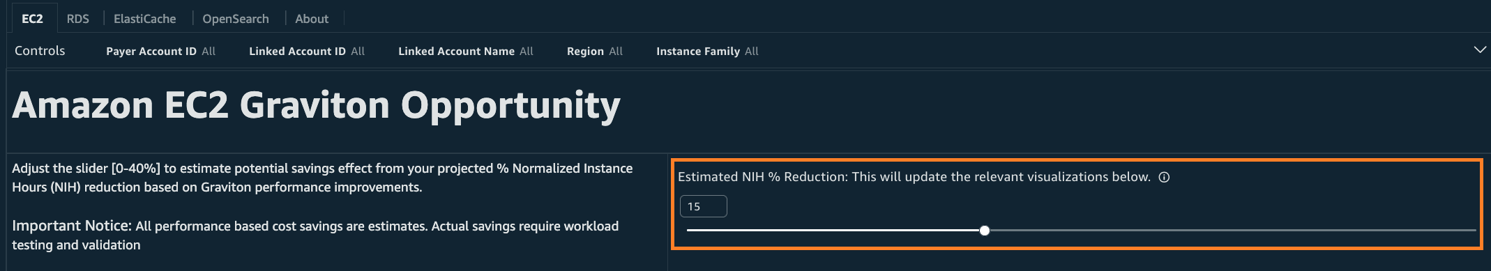
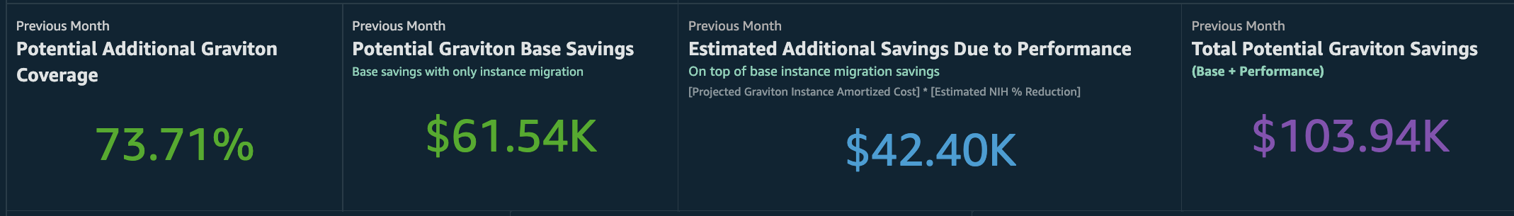

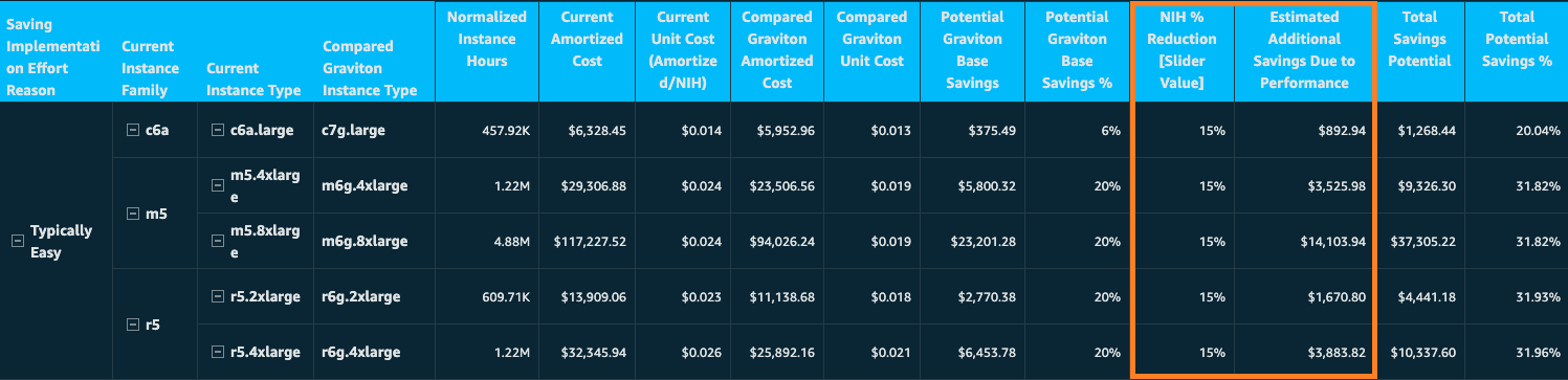
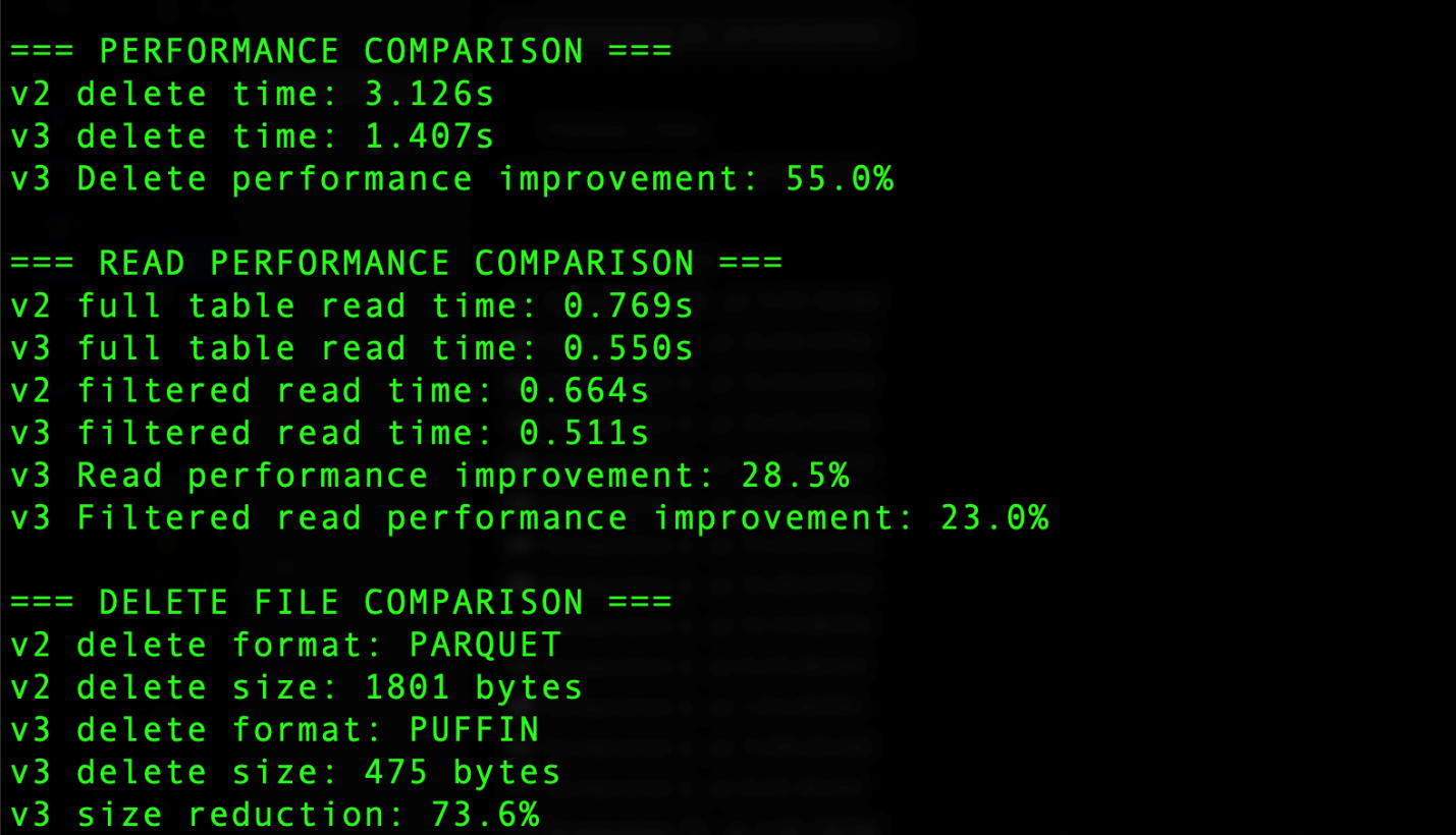
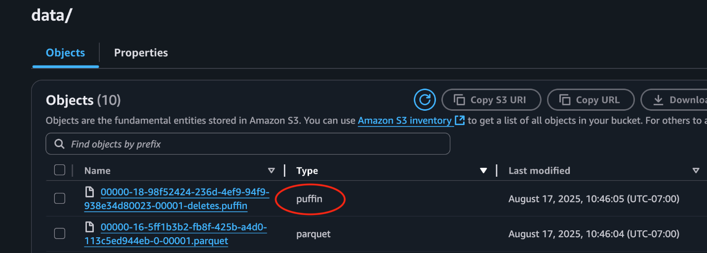


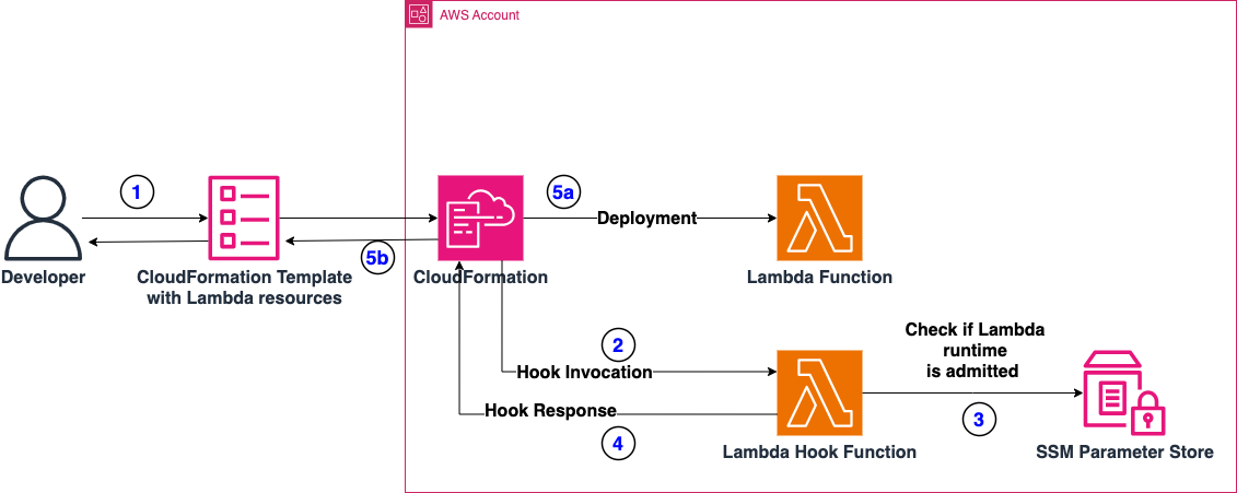
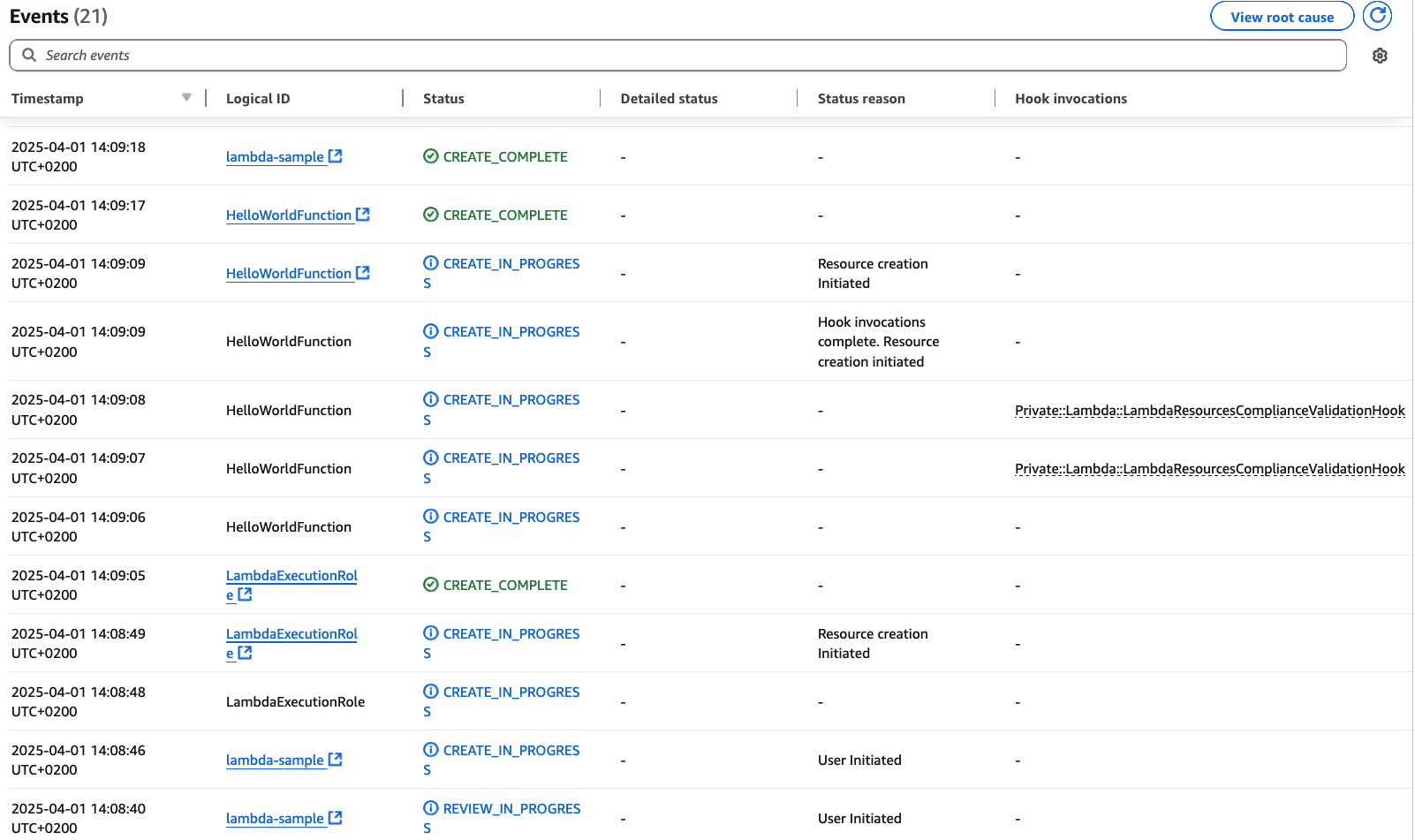
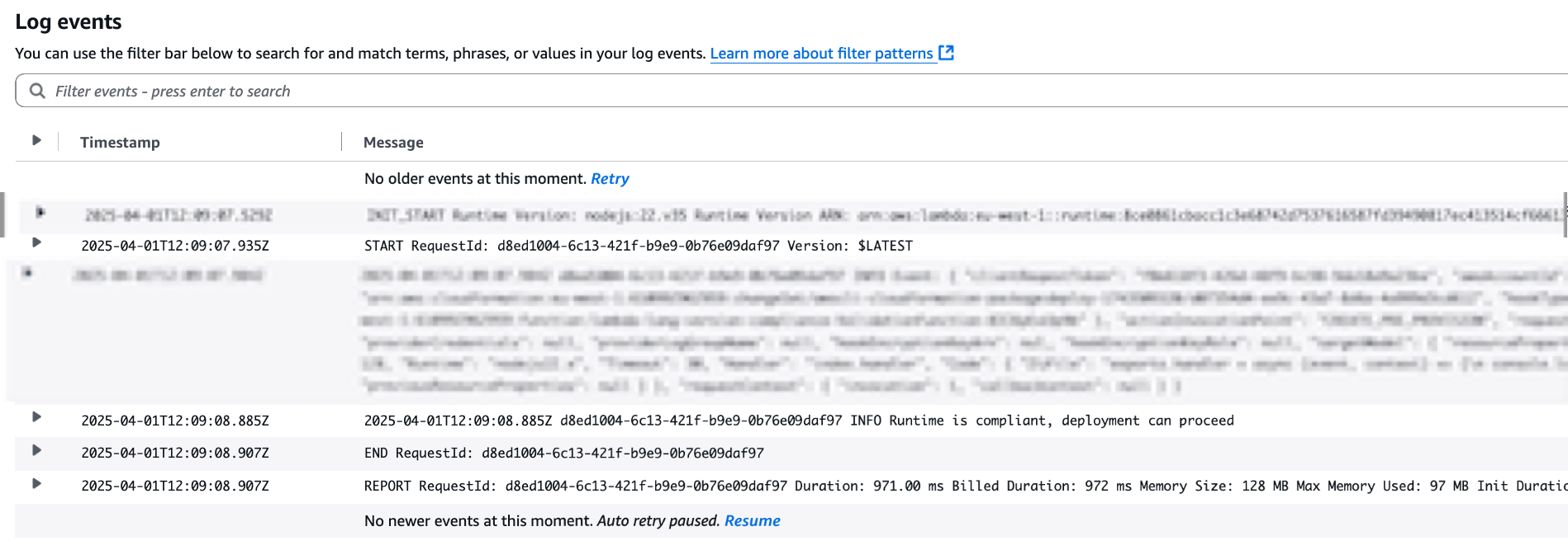
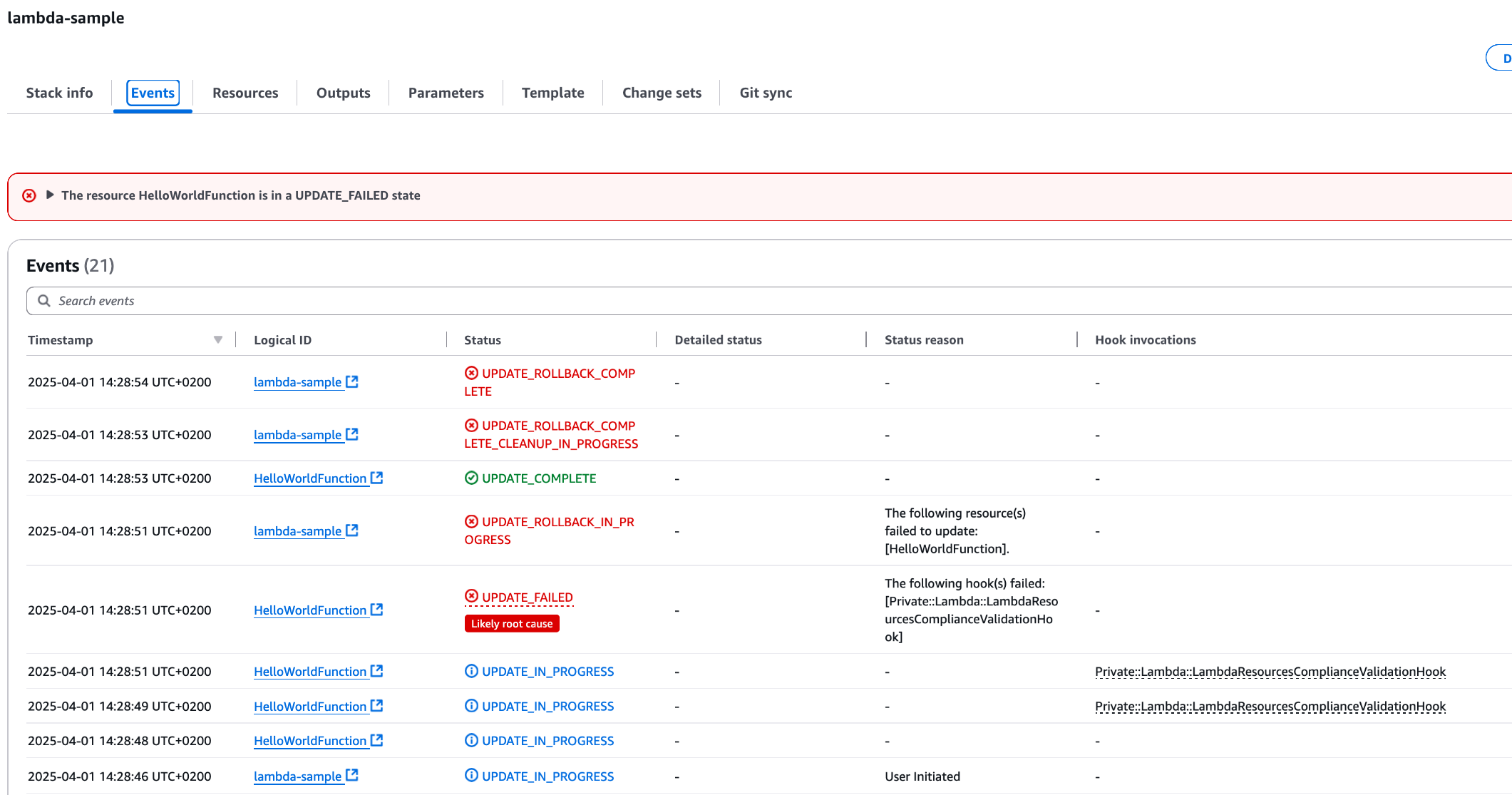
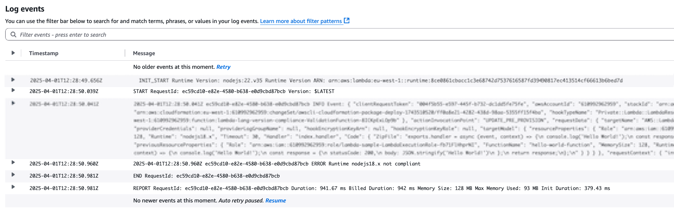


 BP Yau is a Sr Partner Solutions Architect at AWS. His role is to help customers architect big data solutions to process data at scale. Before AWS, he helped Amazon.com Supply Chain Optimization Technologies migrate its Oracle data warehouse to Amazon Redshift and build its next generation big data analytics platform using AWS technologies.
 Saman Irfan is a Senior Specialist Solutions Architect at Amazon Web Services, based in Berlin, Germany. She collaborates with customers across industries to design and implement scalable, high-performance analytics solutions using cloud technologies. Saman is passionate about helping organizations modernize their data architectures and unlock the full potential of their data to drive innovation and business transformation. Outside of work, she enjoys spending time with her family, watching TV series, and staying updated with the latest advancements in technology.
 Raghu Kuppala is an Analytics Specialist Solutions Architect experienced working in the databases, data warehousing, and analytics space. Outside of work, he enjoys trying different cuisines and spending time with his family and friends.
 Neela Kulkarni is a Solutions Architect with Amazon Web Services. She primarily serves independent software vendors in the Northeast US, providing architectural guidance and best practice recommendations for new and existing workloads. Outside of work, she enjoys traveling, swimming, and spending time with her family.


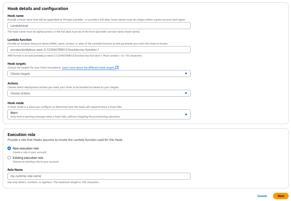


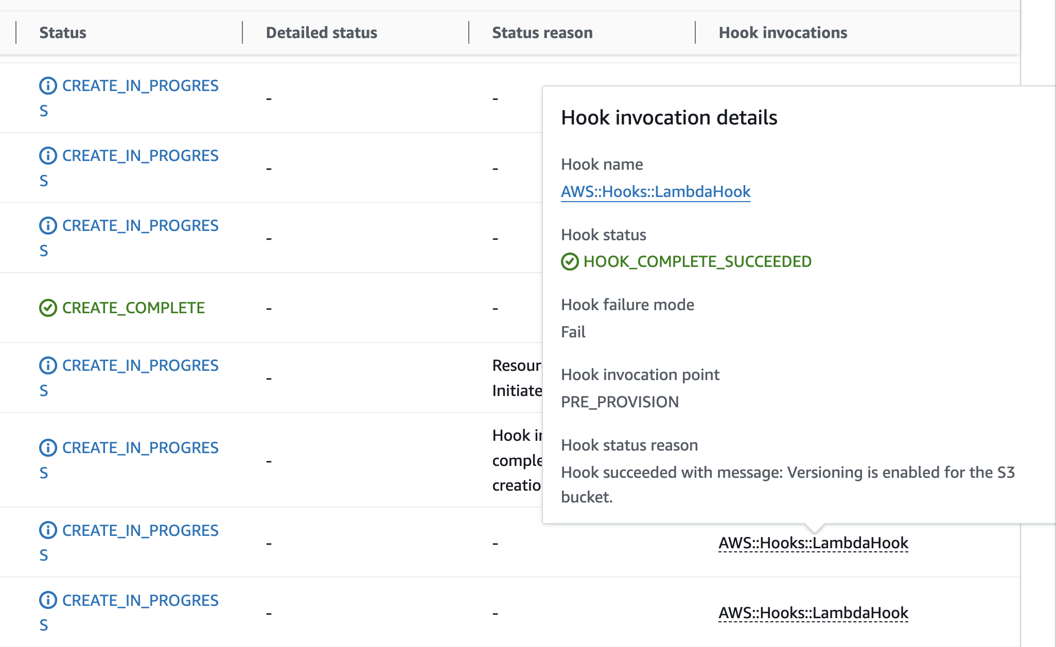

 Stella Hie is a Sr. Product Manager Technical for AWS Infrastructure as Code. She focuses on proactive control and governance space, working on delivering the best experience for customers to use AWS solutions safely. Outside of work, she enjoys hiking, playing piano, and watching live shows.


 Shaheer Mansoor is a Senior Machine Learning Engineer at AWS, where he specializes in developing cutting-edge machine learning platforms. His expertise lies in creating scalable infrastructure to support advanced AI solutions. His focus areas are MLOps, feature stores, data lakes, model hosting, and generative AI.
 Anoop Kumar K M is a Data Architect at AWS with focus in the data and analytics area. He helps customers in building scalable data platforms and in their enterprise data strategy. His areas of interest are data platforms, data analytics, security, file systems and operating systems. Anoop loves to travel and enjoys reading books in the crime fiction and financial domains.
 Sreenivas Nettem is a Lead Database Consultant at AWS Professional Services. He has experience working with Microsoft technologies with a specialization in SQL Server. He works closely with customers to help migrate and modernize their databases to AWS.


 Raks Khare is a Senior Analytics Specialist Solutions Architect at AWS based out of Pennsylvania. He helps customers across varying industries and regions architect data analytics solutions at scale on the AWS platform. Outside of work, he likes exploring new travel and food destinations and spending quality time with his family.
 Blessing Bamiduro is part of the Amazon Redshift Product Management team. She works with customers to help explore the use of Amazon Redshift ML in their data warehouse. In her spare time, Blessing loves travels and adventures.


 Diego Colombatto is a Senior Partner Solutions Architect at AWS. He brings more than 15 years of experience in designing and delivering Digital Transformation projects for enterprises. At AWS, Diego works with partners and customers advising how to leverage AWS technologies to translate business needs into solutions.
 Angel Conde Manjon is a Sr. EMEA Data & AI PSA, based in Madrid. He has previously worked on research related to Data Analytics and Artificial Intelligence in diverse European research projects. In his current role, Angel helps partners develop businesses centered on Data and AI.
 Tiziano Curci is a Manager, EMEA Data & AI PDS at AWS. He leads a team that works with AWS Partners (G/SI and ISV), to leverage the most comprehensive set of capabilities spanning databases, analytics and machine learning, to help customers unlock the through power of data through an end-to-end data strategy.
 Steve Phillips is a senior technical account manager at AWS in the North America region. Steve has worked with games customers for eight years and currently focuses on data warehouse architectural design, data lakes, data ingestion pipelines, and cloud distributed architectures.
 Sudipta Bagchi is a Sr. Specialist Solutions Architect at Amazon Web Services. He has over 14 years of experience in data and analytics, and helps customers design and build scalable and high-performant analytics solutions. Outside of work, he loves running, traveling, and playing cricket.


 testproject-dev: destroyed

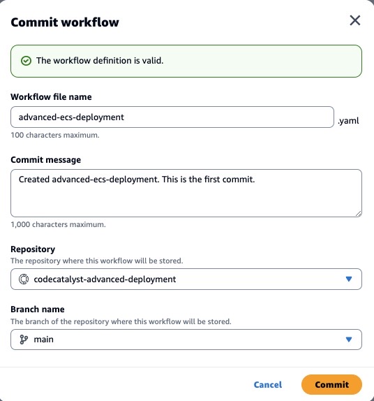
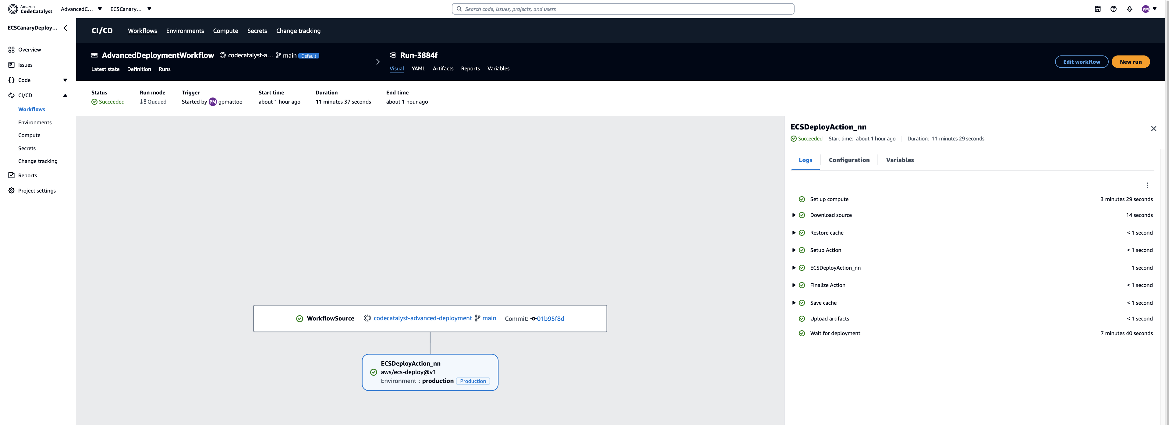


 Aarthi Srinivasan is a Senior Big Data Architect with AWS Lake Formation. She likes building data lake solutions for AWS customers and partners. When not on the keyboard, she explores the latest science and technology trends and spends time with her family.
 Srividya Parthasarathy is a Senior Big Data Architect on the AWS Lake Formation team. She enjoys building analytics and data mesh solutions on AWS and sharing them with the community.


 Babu Srinivasan is a Senior Partner Solutions Architect at MongoDB. In his current role, he is working with AWS to build the technical integrations and reference architectures for the AWS and MongoDB solutions. He has more than two decades of experience in Database and Cloud technologies . He is passionate about providing technical solutions to customers working with multiple Global System Integrators(GSIs) across multiple geographies.
 Robert Walters is currently a Senior Product Manager at MongoDB. Previous to MongoDB, Rob spent 17 years at Microsoft working in various roles, including program management on the SQL Server team, consulting, and technical pre-sales. Rob has co-authored three patents for technologies used within SQL Server and was the lead author of several technical books on SQL Server. Rob is currently an active blogger on MongoDB Blogs.