All posts by Bharav Patel

Cut costs and simplify operations with writable warm storage in Amazon OpenSearch Service

Post Syndicated from Bharav Patel original https://aws.amazon.com/blogs/big-data/cut-costs-and-simplify-operations-with-writable-warm-storage-in-amazon-opensearch-service/

Managing petabytes of search data means making tough choices: keep everything fast and expensive, or make it affordable but read-only. UltraWarm is a proven, cost-effective solution for read-heavy historical data. However, some workloads occasionally need to update historical records, such as late-arriving data or compliance corrections. With UltraWarm, you must migrate those indices back to hot, perform the update, and migrate back. What if you could write directly to your cost-effective warm storage instead?

In this post, I show you how writable warm storage removes the costly migration cycle. You can reduce your infrastructure costs by up to 48 percent and update historical data in seconds instead of hours. I walk through a real-world cost comparison and performance benchmarks, and help you decide when to use writable warm versus UltraWarm.

The challenge with tiered storage

Amazon OpenSearch Service handles data-intensive search and analytics workloads, from real-time log analytics and application monitoring to security event detection. As your data volumes grow from terabytes to petabytes, you face a fundamental question: how do you keep recent data fast while making earlier data affordable?

OpenSearch Service addresses this with a tiered storage architecture:

  • Hot – Highest performance for active indexing and search using instance-attached storage.
  • UltraWarm – Cost-effective, read-only tier backed by Amazon Simple Storage Service (Amazon S3) with local caching for less frequently queried data.
  • Cold – Fully detached from the cluster, with the lowest cost for rarely accessed data. Cold indices must be migrated back to UltraWarm or hot before any reads or writes can be performed.

For immutable log data, this model works well. However, a specific class of workloads hits its limitations when they occasionally need to write to earlier data, and read-only becomes a bottleneck.

Prerequisites

To use writable warm storage, you need the following:

  1. An Amazon OpenSearch Service domain running version 3.3 or later.
  2. OpenSearch Optimized (OI2) instance family support in your AWS Region.
  3. Workloads with a minimum 5-second refresh interval.
  4. Data nodes using the OpenSearch Optimized instance family (OR2 for hot, OI2 for warm).

Note: Writable warm doesn’t currently support the cold storage tier.

The UltraWarm bottleneck

With UltraWarm, updating even a single document requires migrating the index back to hot, performing the write, and migrating it back. This round trip involves a force merge (consolidating index segments), snapshot creation, and shard relocation. These operations consume significant CPU, memory, and disk space on your hot nodes, and they take approximately 130 minutes per 100 GB index. This time was measured on a domain with 3 × r6g.2xlarge hot nodes, 3 × ultrawarm1.large warm nodes, and 3 dedicated leader nodes (US East, N. Virginia), using a single-shard index with one replica. Actual times vary based on domain configuration, shard count, segment count, hot node utilization, and migration queue depth. The result is that you over-provision hot nodes, build complex pipelines, or keep data in hot longer than necessary, which increases cost and complexity.

Introducing writable warm storage

OpenSearch Service now offers writable warm nodes that use OpenSearch Optimized (OI2) instances, the same instance family that powers durable, Amazon S3-backed storage on hot nodes. Because data is already persisted on Amazon S3, tier transitions become a lightweight shard relocation rather than a resource-intensive migration. The Lucene engine, which is OpenSearch’s underlying search library, operates identically on both tiers. As a result, writable warm nodes support active writes, background merges, and periodic refreshes, just like hot nodes.

Late-arriving data, compliance backfills, and corrections that previously required a warm-to-hot-to-warm round trip now resolve with a direct write in seconds. There is no force merge, no snapshot, no shard relocation, and no hot node resource consumption.
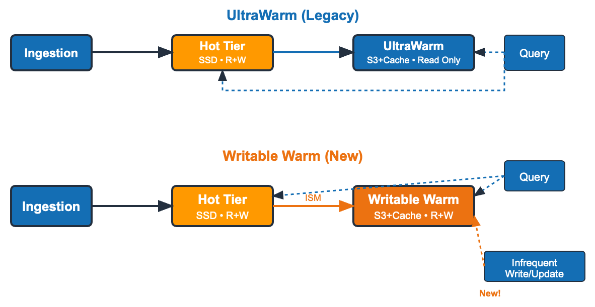
Diagram comparing UltraWarm and writable warm data flows. In the UltraWarm legacy flow, data is ingested into the hot tier, migrated to read-only UltraWarm, and any update requires a round trip back to hot. In the writable warm flow, indices transition from hot to writable warm, which accepts reads and writes directly without migrating back to hot.

UltraWarm (legacy) data flow: Data is ingested into the hot tier (SSD, read and write). Index State Management (ISM) policies migrate indices to UltraWarm (Amazon S3-backed, read-only). Any update requires migrating the index back to hot (dashed arrow), writing, then migrating back.

Writable warm (new) data flow: Same ingestion path through hot, with ISM transitioning indices to writable warm. The key difference is that writable warm supports both reads and writes. Late-arriving updates go directly to warm, with no migration back to hot. Because both tiers use Amazon S3 as durable storage through OpenSearch Optimized instances, transitions are lightweight shard relocations, not resource-intensive migrations.

The benefits: cost, operations, and flexibility

Writable warm delivers advantages in three areas: cost, operational simplicity, and flexibility.

Cost

Unlike UltraWarm, which only offers on-demand pricing, OI2 instances support Reserved Instance (RI) pricing, a commitment-based discount model. By committing to a 1-year or 3-year Reserved Instance, you can save 31–52 percent compared to UltraWarm nodes. This makes writable warm significantly more cost-effective for predictable, long-running workloads. The newly introduced Database savings plan for OpenSearch Service provides savings of around 22 percent over UltraWarm instances. Both tiers use Amazon S3 for durable storage, so node failure means only temporary unavailability, not data loss. For cost-sensitive workloads that can tolerate brief downtime during node recovery, you can configure zero replicas on warm indices to reduce costs further.

Real-world cost comparison

Consider a workload ingesting 2 TB/day with 210 days total retention, where updates can arrive at any point. With UltraWarm’s read-only constraint, you must keep data in hot for 30 days before migrating to warm. With writable warm, updates happen directly on warm, so hot retention drops to only 7 days.

At small scale, the hot tier reduction benefit is modest. Writable warm is still cost-effective if you need write capability on warm data, can commit to RI pricing, or value the operational simplicity of eliminating migration pipelines. For purely immutable data with short retention, UltraWarm on-demand might still be cheaper. Use the AWS Pricing Calculator to model your specific scenario.

The following table shows estimated monthly costs using on-demand and All Upfront Reserved Instance (AURI) pricing in the US East (N. Virginia) Region as of March 2026. For the latest pricing, see Amazon OpenSearch Service pricing on the AWS website.

Component Hot + UltraWarm (30d hot / 180d warm) Hot + writable warm (7d hot / 203d warm)
Hot data nodes $12,264 (21 × or2.2xlarge) $12,264 (21 × or2.2xlarge)
Hot EBS cost $10,212.84 (21 * 3986 GB) $2,636
Hot remote storage $2,008.28 $518
Warm data nodes $39,128 (20× ultrawarm1.large) $50,409 (15× oi2.8xlarge)
Amazon S3 storage $9,504 $1,070
Leader nodes $1,307 (3 × m8g.2xlarge) $1,307 (3 × m8g.2xlarge)
On-demand total $74,427 $69,297
1-year AURI $69,674 $43,918 (~36% less)
3-year AURI $67,367 $34,939 (~48% less)
Database savings plan $71,708 $55,406 (~22%)

Operations

Reclaim hot node capacity. Writable warm removes two common causes of hot node over-provisioning: reserving 35 percent of disk space for force merge operations, and maintaining extra capacity to temporarily move data back to hot for writes. You can run your hot tier at higher utilization, which reduces the number of hot nodes you need.

Simpler migrations. UltraWarm migrations are multi-step operations (force merge, snapshot, and shard relocation) that need careful scheduling during low-traffic windows, and they are limited to 10 queued at a time. Writable warm simplifies this to a lightweight shard relocation, with more straightforward ISM policies and no scheduling constraints.

Flexibility

UltraWarm offers only two instance sizes: ultrawarm1.medium (1.5 TiB) and ultrawarm1.large (20 TiB). Writable warm with OI2 instances offers a full range from oi2.large to oi2.16xlarge. Each size addresses up to 5× its local cache size, so you can right-size warm capacity precisely to your workload.

Search performance

We benchmarked search latency using the NYC Taxis workload, comparing writable warm (oi2.large) against UltraWarm nodes. All measurements are P90 latencies.

On the NYC_TAXIS benchmark, writable warm matched or beat UltraWarm on 6 of 7 query types at P90, including lightweight filters, ranges, sorts, and time-histogram aggregations. For most real-world search patterns, writable warm delivers comparable or better performance than UltraWarm, plus the ability to write directly to the tier.

Search performance: writable warm compared to UltraWarm

Task Writable warm node latency in ms UltraWarm latency in ms UltraWarm vs. writable warm diff %
NYC_TAXIS workload type ** ** ** ** ** **
default (P90) 21.287 23.857 12.07223
range (P90) 21.23 21.016 -1.00718
distance_amount_agg (P90) 5,069 3929.23 -22.48406
autohisto_agg (P90) 21.076 22.002 4.39348
date_histogram_agg (P90) 21.363 21.792 2.01031
desc_sort_tip_amount (P90) 23.224 23.797 2.46636
asc_sort_tip_amount (P90) 22.483 22.482 -0.00445

When to choose what

Should you switch from UltraWarm to writable warm? It depends on your workload.

Requirement Writable Warm UltraWarm
Write enabled Read-only
Reserved Instance pricing
Instance size flexibility Wide range (large–8xlarge) 2 options only
Cold tier support
Need for OpenSearch Optimized instance families
Concurrent tier transitions ✗ (sequential)
Hot node impact during migration Minimal High (CPU/memory)

Clean up resources

If you created a test domain to evaluate writable warm storage, delete it to avoid ongoing charges. In the OpenSearch Service console, select your domain and choose Delete. This removes all nodes and stops Amazon S3 storage charges for that domain.

Summary

In this post, I showed you how writable warm storage eliminates the costly migration cycle that UltraWarm’s read-only limitation creates. You get up to 36 percent cost savings with 1-year Reserved Instances, faster search performance, and a simpler operational model. Writable warm also removes data transitions between tiers, and Reserved Instance pricing becomes available for warm storage for the first time.

Writable warm requires OpenSearch Service version 3.3 or later with OI2 instances. For domains needing cold tier support, earlier OpenSearch Service versions, or non-optimized instance families, UltraWarm remains the right choice.

Next steps: Start by analyzing your current hot and warm split. How many days of data do you keep in hot only to accommodate occasional updates? Use the AWS Pricing Calculator to model your potential savings, and enable writable warm on a test domain in minutes. At the time of this post, writable warm is supported on OpenSearch Service version 3.3. For step-by-step instructions, see Migrating to writable warm storage in the OpenSearch Service documentation.

Have you tried writable warm storage? I’d love to hear about your experience and any questions you have in the comments.


About the author

Bharav Patel

Bharav Patel

Bharav is a Specialist Solution Architect, Analytics at Amazon Web Services. He primarily works on Amazon OpenSearch Service and helps customers with key concepts and design principles of running OpenSearch workloads on the cloud. Bharav likes to explore new places and try out different cuisines.

Build conversational AI search with Amazon OpenSearch Service

Post Syndicated from Bharav Patel original https://aws.amazon.com/blogs/big-data/build-conversational-ai-search-with-amazon-opensearch-service/

Retrieval Augmented Generation (RAG) is a well-known approach to creating generative AI applications. RAG combines large language models (LLMs) with external world knowledge retrieval and is increasingly popular for adding accuracy and personalization to AI. It retrieves relevant information from external sources, augments the input with this data, and generates responses based on both. This approach reduces hallucinations, improves fact accuracy, and allows for up-to-date, efficient, and explainable AI systems. RAG’s ability to break through classical language model limitations has made it applicable to broad AI use cases.

Amazon OpenSearch Service is a versatile search and analytics tool. It is capable of performing security analytics, searching data, analyzing logs, and many other tasks. It can also work with vector data with a k-nearest neighbors (k-NN) plugin, which makes it helpful for more complex search strategies. Because of this feature, OpenSearch Service can serve as a knowledge base for generative AI applications that integrate language generation with search results.

By preserving context over several exchanges, honing responses, and providing a more seamless user experience, conversational search enhances RAG. It helps with complex information needs, resolves ambiguities, and manages multi-turn reasoning. Conversational search provides a more natural and personalized interaction, yielding more accurate and pertinent results, even though standard RAG performs well for single queries.

In this post, we explore conversational search, its architecture, and various ways to implement it.

Solution overview

Let’s walk through the solution to build conversational search. The following diagram illustrates the solution architecture.

The new OpenSearch feature known as agents and tools is used to create conversational search. To develop sophisticated AI applications, agents coordinate a variety of machine learning (ML) tasks. Every agent has a number of tools; each intended for a particular function. To use agents and tools, you need OpenSearch version 2.13 or later.

Prerequisites

To implement this solution, you need an AWS account. If you don’t have one, you can create an account. You also need an OpenSearch Service domain with OpenSearch version 2.13 or later. You can use an existing domain or create a new domain.

To use the Amazon Titan Text Embedding and Anthropic Claude V1 models in Amazon Bedrock, you need to enable access to these foundation models (FMs). For instructions, refer to Add or remove access to Amazon Bedrock foundation models.

Configure IAM permissions

Complete the following steps to set up an AWS Identity and Access Management (IAM) role and user with appropriate permissions:

  1. Create an IAM role with the following policy that will allow the OpenSearch Service domain to invoke the Amazon Bedrock API:
    {
        "Version": "2012-10-17",
        "Statement": [
            {
                "Sid": "Statement1",
                "Effect": "Allow",
                "Action": [
                    "bedrock:InvokeAgent",
                    "bedrock:InvokeModel"
                ],
                "Resource": [
                    "arn:aws:bedrock:${Region}::foundation-model/amazon.titan-embed-text-v1",
                    "arn:aws:bedrock: ${Region}::foundation-model/anthropic.claude-instant-v1"
                ]
            }
        ]
    }
    

Depending on the AWS Region and model you use, specify those in the Resource section.

  1. Add opensearchservice.amazonaws.com as a trusted entity.
  2. Make a note of the IAM role Amazon Resource name (ARN).
  3. Assign the preceding policy to the IAM user that will create a connector.
  4. Create a passRole policy and assign it to IAM user that will create the connector using Python:
    {
        "Version": "2012-10-17",
        "Statement": [
            {
                "Effect": "Allow",
                "Action": "iam:PassRole",
                "Resource": "arn:aws:iam::${AccountId}:role/OpenSearchBedrock"
            }
        ]
    }
  5. Map the IAM role you created to the OpenSearch Service domain role using the following steps:
    • Log in to the OpenSearch Dashboard and open the Security page from the navigation menu.
    • Choose Roles and select ml_all_access.
    • Choose Mapped Users and Manage Mapping.
    • Under Users, add the ARN of the IAM user you created.

Establish a connection to the Amazon Bedrock model using the MLCommons plugin

In order to identify patterns and relationships, an embedding model transforms input data—such as words or images—into numerical vectors in a continuous space. Similar objects are grouped together to make it easier for AI systems to comprehend and respond to intricate user enquiries.

Semantic search concentrates on the purpose and meaning of a query. OpenSearch stores data in a vector index for retrieval and transforms it into dense vectors (lists of numbers) using text embedding models. We are using amazon.titan-embed-text-v1 hosted on Amazon Bedrock, but you will need to evaluate and choose the right model for your use case. The amazon.titan-embed-text-v1 model maps sentences and paragraphs to a 1,536-dimensional dense vector space and is optimized for the task of semantic search.

Complete the following steps to establish a connection to the Amazon Bedrock model using the MLCommons plugin:

  1. Establish a connection by using the Python client with the connection blueprint.
  2. Modify the values of the host and region parameters in the provided code block. For this example, we’re running the program in Visual Studio Code with Python version 3.9.6, but newer versions should also work.
  3. For the role ARN, use the ARN you created earlier, and run the following script using the credentials of the IAM user you created:
    import boto3
    import requests 
    from requests_aws4auth import AWS4Auth
    
    host = 'https://search-test.us-east-1.es.amazonaws.com/'
    region = 'us-east-1'
    service = 'es'
    credentials = boto3.Session().get_credentials()
    awsauth = AWS4Auth(credentials.access_key, credentials.secret_key, region, service, session_token=credentials.token)
    
    path = '_plugins/_ml/connectors/_create'
    url = host + path
    
    payload = {
      "name": "Amazon Bedrock Connector: embedding",
      "description": "The connector to bedrock Titan embedding model",
      "version": 1,
      "protocol": "aws_sigv4",
      "parameters": {
        "region": "us-east-1",
        "service_name": "bedrock",
        "model": "amazon.titan-embed-text-v1"
      },
      "credential": {
        "roleArn": "arn:aws:iam::<accountID>:role/opensearch_bedrock_external"
      },
      "actions": [
        {
          "action_type": "predict",
          "method": "POST",
          "url": "https://bedrock-runtime.${parameters.region}.amazonaws.com/model/${parameters.model}/invoke",
          "headers": {
            "content-type": "application/json",
            "x-amz-content-sha256": "required"
          },
          "request_body": "{ \"inputText\": \"${parameters.inputText}\" }",
          "pre_process_function": "connector.pre_process.bedrock.embedding",
          "post_process_function": "connector.post_process.bedrock.embedding"
        }
      ]
    }
    
    headers = {"Content-Type": "application/json"}
    
    r = requests.post(url, auth=awsauth, json=payload, headers=headers, timeout=15)
    print(r.status_code)
    print(r.text)
    
  4. Run the Python program. This will return connector_id.
    python3 connect_bedrocktitanembedding.py
    200
    {"connector_id":"nbBe65EByVCe3QrFhrQ2"}
  5. Create a model group against which this model will be registered in the OpenSearch Service domain:
    POST /_plugins/_ml/model_groups/_register
    {
      "name": "embedding_model_group",
      "description": "A model group for bedrock embedding models"
    }

    You get the following output:

    {
      "model_group_id": "1rBv65EByVCe3QrFXL6O",
      "status": "CREATED"
    }
  6. Register a model using connector_id and model_group_id:
    POST /_plugins/_ml/models/_register
    {
        "name": "titan_text_embedding_bedrock",
        "function_name": "remote",
        "model_group_id": "1rBv65EByVCe3QrFXL6O",
        "description": "test model",
        "connector_id": "nbBe65EByVCe3QrFhrQ2",
       "interface": {}
    }

You get the following output:

{
  "task_id": "2LB265EByVCe3QrFAb6R",
  "status": "CREATED",
  "model_id": "2bB265EByVCe3QrFAb60"
}
  1. Deploy a model using the model ID:
POST /_plugins/_ml/models/2bB265EByVCe3QrFAb60/_deploy

You get the following output:

{
  "task_id": "bLB665EByVCe3QrF-slA",
  "task_type": "DEPLOY_MODEL",
  "status": "COMPLETED"
}

Now the model is deployed, and you will see that in OpenSearch Dashboards on the OpenSearch Plugins page.

Create an ingestion pipeline for data indexing

Use the following code to create an ingestion pipeline for data indexing. The pipeline will establish a connection to the embedding model, retrieve the embedding, and then store it in the index.

PUT /_ingest/pipeline/cricket_data_pipeline {
    "description": "batting score summary embedding pipeline",
    "processors": [
        {
            "text_embedding": {
                "model_id": "GQOsUJEByVCe3QrFfUNq",
                "field_map": {
                    "cricket_score": "cricket_score_embedding"
                }
            }
        }
    ]
}

Create an index for storing data

Create an index for storing data (for this example, the cricket achievements of batsmen). This index stores raw text and embeddings of the summary text with 1,536 dimensions and uses the ingest pipeline we created in the previous step.

PUT cricket_data {
    "mappings": {
        "properties": {
            "cricket_score": {
                "type": "text"
            },
            "cricket_score_embedding": {
                "type": "knn_vector",
                "dimension": 1536,
                "space_type": "l2",
                "method": {
                    "name": "hnsw",
                    "engine": "faiss"
                }
            }
        }
    },
    "settings": {
        "index": {
            "knn": "true"
        }
    }
}

Ingest sample data

Use the following code to ingest the sample data for four batsmen:

POST _bulk?pipeline=cricket_data_pipeline
{"index": {"_index": "cricket_data"}}
{"cricket_score": "Sachin Tendulkar, often hailed as the 'God of Cricket,' amassed an extraordinary batting record throughout his 24-year international career. In Test cricket, he played 200 matches, scoring a staggering 15,921 runs at an average of 53.78, including 51 centuries and 68 half-centuries, with a highest score of 248 not out. His One Day International (ODI) career was equally impressive, spanning 463 matches where he scored 18,426 runs at an average of 44.83, notching up 49 centuries and 96 half-centuries, with a top score of 200 not out – the first double century in ODI history. Although he played just one T20 International, scoring 10 runs, his overall batting statistics across formats solidified his status as one of cricket's all-time greats, setting numerous records that stand to this day."}
{"index": {"_index": "cricket_data"}}
{"cricket_score": "Virat Kohli, widely regarded as one of the finest batsmen of his generation, has amassed impressive statistics across all formats of international cricket. As of April 2024, in Test cricket, he has scored over 8,000 runs with an average exceeding 50, including numerous centuries. His One Day International (ODI) record is particularly stellar, with more than 12,000 runs at an average well above 50, featuring over 40 centuries. In T20 Internationals, Kohli has maintained a high average and scored over 3,000 runs. Known for his exceptional ability to chase down targets in limited-overs cricket, Kohli has consistently ranked among the top batsmen in ICC rankings and has broken several batting records throughout his career, cementing his status as a modern cricket legend."}
{"index": {"_index": "cricket_data"}}
{"cricket_score": "Adam Gilchrist, the legendary Australian wicketkeeper-batsman, had an exceptional batting record across formats during his international career from 1996 to 2008. In Test cricket, Gilchrist scored 5,570 runs in 96 matches at an impressive average of 47.60, including 17 centuries and 26 half-centuries, with a highest score of 204 not out. His One Day International (ODI) record was equally remarkable, amassing 9,619 runs in 287 matches at an average of 35.89, with 16 centuries and 55 half-centuries, and a top score of 172. Gilchrist's aggressive batting style and ability to change the course of a game quickly made him one of the most feared batsmen of his era. Although his T20 International career was brief, his overall batting statistics, combined with his wicketkeeping skills, established him as one of cricket's greatest wicketkeeper-batsmen."}
{"index": {"_index": "cricket_data"}}
{"cricket_score": "Brian Lara, the legendary West Indian batsman, had an extraordinary batting record in international cricket during his career from 1990 to 2007. In Test cricket, Lara amassed 11,953 runs in 131 matches at an impressive average of 52.88, including 34 centuries and 48 half-centuries. He holds the record for the highest individual score in a Test innings with 400 not out, as well as the highest first-class score of 501 not out. In One Day Internationals (ODIs), Lara scored 10,405 runs in 299 matches at an average of 40.48, with 19 centuries and 63 half-centuries. His highest ODI score was 169. Known for his elegant batting style and ability to play long innings, Lara's exceptional performances, particularly in Test cricket, cemented his status as one of the greatest batsmen in the history of the game."}

Deploy the LLM for response generation

Use the following code to deploy the LLM for response generation. Modify the values of host, region, and roleArn in the provided code block.

  1. Create a connector by running the following Python program. Run the script using the credentials of the IAM user created earlier.
    import boto3
    import requests 
    from requests_aws4auth import AWS4Auth
    
    host = 'https://search-test.us-east-1.es.amazonaws.com/'
    region = 'us-east-1'
    service = 'es'
    credentials = boto3.Session().get_credentials()
    awsauth = AWS4Auth(credentials.access_key, credentials.secret_key, region, service, session_token=credentials.token)
    
    path = '_plugins/_ml/connectors/_create'
    url = host + path
    
    payload = {
      "name": "BedRock Claude instant-v1 Connector ",
      "description": "The connector to BedRock service for claude model",
      "version": 1,
      "protocol": "aws_sigv4",
      "parameters": {
        "region": "us-east-1",
        "service_name": "bedrock",
        "anthropic_version": "bedrock-2023-05-31",
        "max_tokens_to_sample": 8000,
        "temperature": 0.0001,
        "response_filter": "$.completion"
      },
       "credential": {
            "roleArn": "arn:aws:iam::accountId:role/opensearch_bedrock_external"
        },
      "actions": [
        {
          "action_type": "predict",
          "method": "POST",
          "url": "https://bedrock-runtime.${parameters.region}.amazonaws.com/model/anthropic.claude-instant-v1/invoke",
          "headers": {
            "content-type": "application/json",
            "x-amz-content-sha256": "required"
          },
          "request_body": "{\"prompt\":\"${parameters.prompt}\", \"max_tokens_to_sample\":${parameters.max_tokens_to_sample}, \"temperature\":${parameters.temperature},  \"anthropic_version\":\"${parameters.anthropic_version}\" }"
        }
      ]
     }
        
    
    headers = {"Content-Type": "application/json"}
    
    r = requests.post(url, auth=awsauth, json=payload, headers=headers, timeout=15)
    print(r.status_code)
    print(r.text)

If it ran successfully, it would return connector_id and a 200-response code:

200
{"connector_id":"LhLSZ5MBLD0avmh1El6Q"}
  1. Create a model group for this model:
    POST /_plugins/_ml/model_groups/_register
    {
        "name": "claude_model_group",
        "description": "This is an example description"
    }

This will return model_group_id; make a note of it:

{
  "model_group_id": "LxLTZ5MBLD0avmh1wV4L",
  "status": "CREATED"
}
  1. Register a model using connection_id and model_group_id:
    POST /_plugins/_ml/models/_register
    {
        "name": "anthropic.claude-v1",
        "function_name": "remote",
        "model_group_id": "LxLTZ5MBLD0avmh1wV4L",
        "description": "LLM model",
        "connector_id": "LhLSZ5MBLD0avmh1El6Q",
        "interface": {}
    }
    

It will return model_id and task_id:

{
  "task_id": "YvbVZ5MBtVAPFbeA7ou7",
  "status": "CREATED",
  "model_id": "Y_bVZ5MBtVAPFbeA7ovb"
}
  1. Finally, deploy the model using an API:
POST /_plugins/_ml/models/Y_bVZ5MBtVAPFbeA7ovb/_deploy

The status will show as COMPLETED. That means the model is successfully deployed.

{
  "task_id": "efbvZ5MBtVAPFbeA7otB",
  "task_type": "DEPLOY_MODEL",
  "status": "COMPLETED"
}

Create an agent in OpenSearch Service

An agent orchestrates and runs ML models and tools. A tool performs a set of specific tasks. For this post, we use the following tools:

  • VectorDBTool – The agent use this tool to retrieve OpenSearch documents relevant to the user question
  • MLModelTool – This tool generates user responses based on prompts and OpenSearch documents

Use the embedding model_id in VectorDBTool and LLM model_id in MLModelTool:

POST /_plugins/_ml/agents/_register {
    "name": "cricket score data analysis agent",
    "type": "conversational_flow",
    "description": "This is a demo agent for cricket data analysis",
    "app_type": "rag",
    "memory": {
        "type": "conversation_index"
    },
    "tools": [
        {
            "type": "VectorDBTool",
            "name": "cricket_knowledge_base",
            "parameters": {
                "model_id": "2bB265EByVCe3QrFAb60",
                "index": "cricket_data",
                "embedding_field": "cricket_score_embedding",
                "source_field": [
                    "cricket_score"
                ],
                "input": "${parameters.question}"
            }
        },
        {
            "type": "MLModelTool",
            "name": "bedrock_claude_model",
            "description": "A general tool to answer any question",
            "parameters": {
                "model_id": "gbcfIpEByVCe3QrFClUp",
                "prompt": "\n\nHuman:You are a professional data analysist. You will always answer question based on the given context first. If the answer is not directly shown in the context, you will analyze the data and find the answer. If you don't know the answer, just say don't know. \n\nContext:\n${parameters.cricket_knowledge_base.output:-}\n\n${parameters.chat_history:-}\n\nHuman:${parameters.question}\n\nAssistant:"
            }
        }
    ]
}

This returns an agent ID; take note of the agent ID, which will be used in subsequent APIs.

Query the index

We have batting scores of four batsmen in the index. For the first query, let’s specify the player name:

POST /_plugins/_ml/agents/<agent ID>/_execute {
    "parameters": {
        "question": "What is batting score of Sachin Tendulkar ?"
    }
}

Based on context and available information, it returns the batting score of Sachin Tendulkar. Note the memory_id from the response; you will need it for subsequent questions in the next steps.

We can ask a follow-up question. This time, we don’t specify the player name and expect it to answer based on the earlier question:

POST /_plugins/_ml/agents/<agent ID>/_execute {
    "parameters": {
        "question": " How many T20 international match did he play?",
        "next_action": "then compare with Virat Kohlis score",
        "memory_id": "so-vAJMByVCe3QrFYO7j",
        "message_history_limit": 5,
        "prompt": "\n\nHuman:You are a professional data analysist. You will always answer question based on the given context first. If the answer is not directly shown in the context, you will analyze the data and find the answer. If you don't know the answer, just say don't know. \n\nContext:\n${parameters.population_knowledge_base.output:-}\n\n${parameters.chat_history:-}\n\nHuman:always learn useful information from chat history\nHuman:${parameters.question}, ${parameters.next_action}\n\nAssistant:"
    }
}

In the preceding API, we use the following parameters:

  • Question and Next_action – We also pass the next action to compare Sachin’s score with Virat’s score.
  • Memory_id – This is memory assigned to this conversation. Use the same memory_id for subsequent questions.
  • Prompt – This is the prompt you give to the LLM. It includes the user’s question and the next action. The LLM should answer only using the data indexed in OpenSearch and must not invent any information. This way, you prevent hallucination.

Refer to ML Model tool for more details about setting up these parameters and the GitHub repo for blueprints for remote inferences.

The tool stores the conversation history of the questions and answers in the OpenSearch index, which is used to refine answers by asking follow-up questions.

In real-world scenarios, you can map memory_id against the user’s profile to preserve the context and isolate the user’s conversation history.

We have demonstrated how to create a conversational search application using the built-in features of OpenSearch Service.

Clean up

To avoid incurring future charges, delete the resources created while building this solution:

  1. Delete the OpenSearch Service domain.
  2. Delete the connector.
  3. Delete the index.

Conclusion

In this post, we demonstrated how to use OpenSearch agents and tools to create a RAG pipeline with conversational search. By integrating with ML models, vectorizing questions, and interacting with LLMs to improve prompts, this configuration oversees the entire process. This method allows you to quickly develop AI assistants that are ready for production without having to start from scratch.

If you’re building a RAG pipeline with conversational history to let users ask follow-up questions for more refined answers, give it a try and share your feedback or questions in the comments!


About the author

Bharav Patel is a Specialist Solution Architect, Analytics at Amazon Web Services. He primarily works on Amazon OpenSearch Service and helps customers with key concepts and design principles of running OpenSearch workloads on the cloud. Bharav likes to explore new places and try out different cuisines.

Use the reverse token filter to enable suffix matching queries in OpenSearch

Post Syndicated from Bharav Patel original https://aws.amazon.com/blogs/big-data/use-the-reverse-token-filter-to-enable-suffix-matching-queries-in-opensearch/

OpenSearch is an open-source RESTful search engine built on top of the Apache Lucene library. OpenSearch full-text search is fast, can give the result of complex queries within a fraction of a second. With OpenSearch, you can convert unstructured text into structured text using different text analyzers, tokenizers, and filters to improve search. OpenSearch uses a default analyzer, called the standard analyzer, which works well for most use cases out of the box. But for some use cases, it may not work best, and you need to use a specific analyzer.

In this post, we show how you can implement a suffix-based search. To find a document with the movie name “saving private ryan” for example, you can use the prefix “saving” with a prefix-based query. Occasionally, you also want to match suffixes as well, such as matching “Harry Potter Goblet of Fire” with the suffix “Fire” To do that, first reverse the string “eriF telboG rettoP yrraH” with the reverse token filter, then query for the prefix “eriF”.

Solution overview

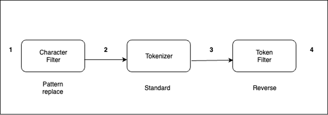
Text analysis involves transforming unstructured text, such as the content of an email or a product description, into a structured format that is finely tuned for effective searching. An analyzer enables the implementation of full-text search using tokenization, which entails breaking down a text into smaller fragments known as tokens, with these tokens commonly representing individual words. To implement a reversed field search, the analyzer does the following.

The analyzer processes text in the following order:

  1. Use a character filter to replace - with _. For example, from “My Driving License Number Is 123-456-789” to “My Driving License Number Is 123_456_789.”
  2. The standard tokenizer splits texts into tokens. For example, from “My Driving License Number Is 123_456_789” to “[ my, driving, license, number, is, 123, 456, 789 ].”
  3. The reverse token filter reverses each token in a stream. For example, from [ my, driving, license, number, is, 123, 456, 789 ] to [ ym, gnivird, esnecil, rebmun, si, 321, 654, 987 ].

The standard analyzer (default analyzer) breaks down input strings into tokens based on word boundaries and removes most punctuation marks. For additional information about analyzers, refer Build-in analyzers.

Indexing and searching

Every document is a collection of fields, each having its own specific data type. When you create a mapping for your data, you create a mapping definition, which contains a list of fields that are pertinent to the document. To know more about index mappings refer to index mapping.

Let’s take the example of an analyzer with the reverse token filter applied on the text field.

  1. First, create an index with mappings as shown in the following code. The new field ‘reverse_title’ is derived from ‘title’ field for suffix search and original field ‘title’ will be used for normal search.
PUT movies
{
  "settings" : {
    "analysis" : {
      "analyzer" : {
        "whitespace_reverse" : {
          "tokenizer" : "whitespace",
          "filter" : ["reverse"]
        }
      }
    }
  },
  "mappings": {
    "properties": {
      "title": { 
        "type": "text",
        "analyzer": "standard",
        "copy_to": "reverse_title"
      },
      "reverse_title": {
        "type": "text",
        "analyzer": "whitespace_reverse"
      }
    }
  }
}

  1. Insert some documents into the index:
POST _bulk
{ "index" : { "_index" : "movies", "_id" : "1" } }
{ "title": "Harry Potter Goblet of Fire" }
{ "index" : { "_index" : "movies", "_id" : "2" } }
{ "title": "Lord of the rings" }
{ "index" : { "_index" : "movies", "_id" : "3" } }
{ "title": "Saving Private Ryan" }
  1. Run the following query to perform a suffix/reverse search on derived field ‘reverse_title’ for “Fire”:
GET movies/_search
{
  "query": {
    "prefix": {
      "reverse_title": {
        "value": "eriF"
      }
    }
  }
}

The following code shows our results:

   {
        "_index": "movies",
        "_id": "1",
        "_score": 1,
        "_source": {
          "title": "Harry Potter Goblet of Fire"
        }
      }
  1. For non-reverse search you can use original field ‘title’.
GET movies/_search
{
  "query": {
    "match": {
      "title": "Fire"
    }
  }
}

The following code shows our result.

{
        "_index": "movies",
        "_id": "1",
        "_score": 0.2876821,
        "_source": {
          "title": "Harry Potter Goblet of Fire"
        }
}

The query returns a document with the movie name “Harry Potter Goblet of Fire”.
If you’re curious to know how search works at high level, refer to A query, or There and Back Again.

Conclusion

In this post, you walked through how text analysis works in OpenSearch and how to implement suffix-based search using a reverse token filter effectively.

If you have feedback about this post, submit your comments in the comments section.


About the Authors

Bharav Patel is a Specialist Solution Architect, Analytics at Amazon Web Services. He primarily works on Amazon OpenSearch Service and helps customers with key concepts and design principles of running OpenSearch workloads on the cloud. Bharav likes to explore new places and try out different cuisines.