Tag Archives: Amazon OpenSearch Service

AWS Weekly Roundup: OpenAI GPT-6 Astra on Amazon Bedrock, Amazon Quick desktop GA, Kiro for students, and more (September 14, 2026)

Post Syndicated from Micah Walter original https://aws.amazon.com/blogs/aws/aws-weekly-roundup-openai-gpt-6-astra-on-amazon-bedrock-amazon-quick-desktop-ga-kiro-for-students-and-more-september-14-2026/

There’s a particular energy to mid-September in New York. Pumpkin spice lattes are flowing, temperatures are dropping, and it’s nearly sweater weather. The city is back at full speed, and so is the AWS launch calendar. This week that energy showed up in a new frontier model on Amazon Bedrock, a desktop app for Amazon Quick, and a reminder that the developers seeing the biggest gains from AI agents aren’t just using better tools — they’re working differently.

Let’s dive in.

Headlines
OpenAI GPT-6 Astra is now generally available on Amazon Bedrock – GPT-6 Astra is OpenAI’s latest and most capable model to date, and you can now run it on Amazon Bedrock. It brings deeper reasoning and judgment, professional-quality writing and design, and advanced computer and browser use to demanding business workflows. The model supports a context window of up to 1 million input tokens, so you can send it large codebases, long contracts, or extensive document collections and ask it to reconcile competing inputs.

You can call GPT-6 Astra through supported Amazon Bedrock APIs, or configure ChatGPT Work and Codex to use the model on Amazon Bedrock. Alongside the launch, OpenAI is introducing new enterprise plugins for ChatGPT Work that extend Astra’s browser-use capabilities across common business applications. Established AWS controls help you secure workloads, govern access, and audit model invocation activity, and your inference data isn’t used for model training. Read more

Last week’s launches
Here are some launches and updates from this past week that caught my attention:

  • Amazon Quick desktop app is now generally available on macOS and Windows – The Amazon Quick desktop app brings Amazon Quick to your computer, where it can work with local files and stay connected to your calendar, email, and business apps in the background. Conversations, context, and agents stay synchronized across desktop and mobile, so work you start on one surface carries over to the other. With this release, Quick agents also keep running after you close your computer, which means you can start a long-running task before you leave the office, add input from the mobile app on the way home, and review the result when you get there. Existing Quick users can download the desktop app, and the mobile app is available from the Apple App Store and Google Play. Read more
  • AWS Lambda now supports a 90-minute function timeout on Lambda Managed Instances – You can now configure a function timeout of up to 90 minutes for asynchronous and event source mapping (ESM) invocations on Lambda Managed Instances, a 6x increase from the previous 15-minute limit. That opens the door to data processing, media transcoding, financial calculations, AI inference, and batch jobs that need longer continuous execution, without splitting the work across multiple functions. Synchronous invocations keep the existing 15-minute maximum. The longer timeout also applies to steps inside Lambda durable functions, which can still run for up to a year when invoked asynchronously. Read more
  • Amazon EBS Volume Clones now copies volumes across accounts – Amazon Elastic Block Store (Amazon EBS) Volume Clones can now copy a volume into another AWS account and re-encrypt it with an AWS Key Management Service (AWS KMS) key in the target account. If you keep production and development in separate accounts, you can share a volume with AWS Resource Access Manager (AWS RAM) and let the target account create a fresh copy in the same Availability Zone, for example, cloning a production database volume into an isolated development account. Cross-account copy works for all volume types, including unencrypted volumes and volumes encrypted with customer managed keys. Read more
  • Second-generation single-rack AWS Outposts is now generally available – The new single-rack AWS Outposts is a self-contained 42U rack that puts compute, storage, and networking into one compact unit for locations that need low latency, local data processing, or data residency, and don’t have room for a larger footprint. A single rack delivers up to 2,688 vCPU and 100 TB of Amazon EBS storage, and supports the latest x86-powered Amazon EC2 instances, including general purpose (M7i, M8i), compute-optimized (C7i, C8i), memory-optimized (R7i, R8i), and Outposts accelerated networking instances. You get the same APIs, console, automation, governance, and security controls as multi-rack Outposts and AWS Regions. Read more
  • Amazon OpenSearch Serverless is now available on v0 by Vercel – You can now describe a search or AI application in natural language inside v0 by Vercel and get a full-stack app backed by Amazon OpenSearch Serverless. v0 provisions a collection, indexes your data, and uses the OpenSearch Serverless endpoint for full-text search and vector search for retrieval-augmented generation (RAG) workloads, without leaving the v0 interface. OpenSearch Serverless scales capacity up and down for you, so you can focus on the application instead of cluster management. You can provision under a new AWS account or link an existing one. Read more
  • AWS Transform for .NET modernization is now generally available via CLI – You can trigger an AWS-managed .NET modernization in AWS Transform custom with a single CLI command, then run it interactively or script it into an existing pipeline. The CLI sits alongside the existing AWS Transform for .NET experiences in the web application, Visual Studio IDE, Kiro Power, and MCP agents. Use it to upgrade language versions, migrate frameworks, optimize performance, and analyze codebases with transformations you can run as-is or customize. The .NET modernization transformation includes 50,000 free agent minutes per month. Read more

For a full list of AWS announcements, be sure to keep an eye on the What’s New with AWS page.

Other AWS news
Here are some additional posts and resources that you might find interesting:

  • Clare Liguori on frontier engineering – If you already use an AI coding assistant but don’t feel like you’re shipping much faster, start here. Clare Liguori, Senior Principal Engineer at AWS, published a practitioner’s manifesto on frontier engineering: ten principles, drawn from teams across Amazon, for changing how you build software with AI agents. The argument is direct. Software development has split in two, people who changed how they work with agents, and people who only changed their coding tools. Frontier engineering is not vibe coding. You spend the first weeks writing steering files, refactoring the codebase, and learning to decompose work for agents. Those weeks feel slower. The weeks after feel dramatically faster, because you’re no longer building the software directly — you’re building the agent setup that builds the software.
  • A free year of Kiro for students around the world – The Kiro Students program is expanding from 11 universities to 121 new schools across 16 countries. Eligible students get one year of Kiro with 1,000 credits per month and full access to paid features such as premium models and Kiro Web, no credit card and no trial timer. You can work in the IDE, the CLI, Kiro Web in a browser, or Kiro Crew. If you’re a student, sign up with your university email.
  • The state of AI for security: measuring what matters for trust – Security teams are using AI for triage, threat modeling, incident response, and code review, but a tool that flags everything doesn’t save time. In The state of AI for security, Anshumali Shrivastava and Neha Rungta introduce Deception Benchmark, a new evaluation that tests whether a model can tell a real vulnerability from code that looks risky but is actually safe. The benchmark includes 14,822 samples across 16 languages and more than 70 Common Weakness Enumeration (CWE) categories. Under standard prompting, precision landed in the mid-50s, about as likely to be inaccurate as accurate, and none of the 12 models tested kept both false positives and false negatives below 10 percent. The post links to the dataset, whitepaper, and submission workflow for verified scoring.
  • Build full-stack AWS applications in minutes with AI-powered scaffolding – Version 1.0 of the Nx Plugin for AWS is an open source toolkit of deterministic generators for APIs, websites, databases, and AI agents, plus the AWS infrastructure to run them. Each generator writes working, deployable code with security, observability, and type-safety already in place, so an AI assistant can assemble the foundation and spend its effort on your application logic. Bingo Industries used it to take a multi-agent operations chatbot from idea to production in less than 3 weeks. The plugin is open source on GitHub. Create a workspace with pnpm create @aws/nx-workspace and point your coding agent at the included MCP server.
  • The oldest architecture in computing – On All Things Distributed, Werner Vogels starts from a question customers always ask “Will AI take my job?”, and lands on memory. After spending time with Kiro Crew, he traces a line from Jeff Hawkins’ A Thousand Brains to how Crew stores, consolidates, and forgets across markdown files, a vector database, and a key-value index. His conclusion: the brain is the oldest architecture in computing, and the people who think hardest about how it works will build the next tools. Now, go build.

For a full list of AWS blog posts, be sure to keep an eye on the AWS Blogs page.

Upcoming AWS events
Check your calendar and sign up for upcoming AWS events:

Join the AWS Builder Center to connect with builders, share solutions, and access content that supports your development. Browse here for upcoming AWS-led in-person and virtual events and developer-focused events.

That’s all for this week. Check back next Monday for another Weekly Roundup!

— Micah

This post is part of our Weekly Roundup series. Check back each week for a quick roundup of interesting news and announcements from AWS!

Observing and evaluating production agents using OpenSearch Agent Health

Post Syndicated from Ulrich Hinze original https://aws.amazon.com/blogs/big-data/observing-and-evaluating-production-agents-using-opensearch-agent-health/

As AI agents are moving from experimental prototypes to production workloads, teams need visibility into what agents are doing and a systematic way to measure whether they’re doing it well. Traditional testing methodologies like unit and integration tests fall short for this task, as measuring an agent’s quality isn’t a straightforward true/false decision. Instead, agent observability and evaluations (evals for short) provide a two-legged solution to this problem. Agent observability captures the details of an agent’s behavior, and evals compare this behavior to the behavior that you want. With this approach, teams can monitor their agent’s quality over time and introduce agent-specific quality gates in their software development lifecycle.

In this post, we show how to combine an AI agent running on AWS with OpenSearch Agent Health for observability and evals. You will deploy an agent and its observability data pipeline to AWS, then use Agent Health as a local development tool connecting to your cloud resources.

Overview of solution

Agent observability and evaluations rely on OpenTelemetry traces to understand agent behavior. Traces describe the flow of a request through components of a system. OpenSearch Agent Health is a purpose-built tool for analyzing agent traces and running evaluations against an agent for quality control. Although Agent Health works with any open source OpenSearch installation, many AWS customers choose Amazon OpenSearch Ingestion and Amazon OpenSearch Service for ingesting and storing their OpenTelemetry data. You can connect OpenSearch Agent Health to these AWS resources to fetch live data and store its own configuration and evaluation history.

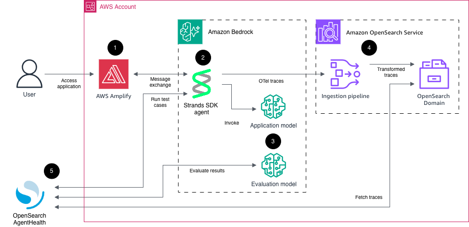
The following diagram shows the overall architecture of the solution presented in this post: Architecture diagram showing the agent, Amazon OpenSearch Ingestion, Amazon OpenSearch Service, and OpenSearch Agent Health observability and evaluation flow

Figure 1: Solution overview

The individual parts are:

  1. AWS Amplify for hosting an assistant-ui chat interface. Connects to the agent backend using the Agent-User Interaction (AG-UI) protocol.
  2. Sample ecommerce AI agent using Strands Agents SDK, deployed to Amazon Bedrock AgentCore runtime, exposing an AG-UI Server-Sent Events (SSE) endpoint. This agent has access to multiple tools, such as product search and shopping basket operations. For this sample project, the tool calls are all simulated within the agent runtime rather than including API calls to other systems. The agent emits messages, reasoning steps, and tool calls as OpenTelemetry traces.
  3. Large language models (LLMs) on Amazon Bedrock. One model (Amazon Nova 2 Lite) is used to power the agent, the other model (Anthropic Claude Opus 4.6) is used to evaluate the agent behavior.
  4. Amazon OpenSearch Ingestion for collecting and transforming the raw agent traces and loading them into an Amazon OpenSearch Service domain. Agent traces have the same structure as regular OpenTelemetry traces, with the addition of generative AI semantics (for example, tool calls and token usage). This means a regular OpenTelemetry pipeline configuration can be used to process agent traces.
  5. OpenSearch Agent Health for analyzing traces and running evaluation test cases and benchmarks against the agent. Agent Health uses the same AG-UI endpoint as the front-end application. It authenticates to the application, to Amazon Bedrock for model functionality, and to Amazon OpenSearch Service using AWS SigV4 authentication.

Walkthrough

In this walkthrough, we showcase how you can use Agent Health and Strands to measure and improve your agent’s quality over time.

We follow these steps:

  • Deploy solution to AWS and test the application.
  • Start Agent Health locally and connect it to cloud resources.
  • Explore agent traces and run evaluations.

We have created a GitHub repository for you to follow along.

Prerequisites

For this walkthrough, you should have the following prerequisites:

  • An AWS account
  • Git
  • Node.js
  • AWS Cloud Development Kit (AWS CDK)

Deploy solution to AWS and test the application

In this section, you check out the repository and deploy the infrastructure to AWS. Be aware that these steps create AWS resources that incur cost. We cover cleanup steps at the end of this post.

First, clone the repository to a local directory:

git clone https://github.com/aws-samples/sample-agent-health-with-amazon-opensearch-service && cd sample-agent-health-with-amazon-opensearch-service

Switch to the infra folder and install dependencies:

cd infra && npm install

Before you can start the deployment, determine the AWS Identity and Access Management (IAM) user or role that you will use to start Agent Health later on. In many cases, this will be the same role that you use to deploy the infrastructure. Set this ARN in your environment by issuing the following command:

export AGENT_HEALTH_READER_ARN=arn:aws:iam::<YOUR_ACCOUNT_ID>:role/<YOUR_ROLE_NAME>

Bootstrap your AWS account for use with AWS CDK:

cdk bootstrap -c agentHealthReaderArn=$AGENT_HEALTH_READER_ARN

Run the infrastructure deployment. Review and acknowledge IAM statement changes when prompted. This takes around 25 minutes to complete:

cdk deploy -R -c agentHealthReaderArn=$AGENT_HEALTH_READER_ARN

The -R parameter defines that if something fails during this deployment, the successfully provisioned resources are retained. Be aware that this command creates AWS resources, incurring cost. Review the cleanup section at the end of this post for removing all created resources.

When the deploy command finishes successfully, you should see an output like the following:

...
AgentObservabilityStack

✨ Deployment time: 1402.42 s

Outputs:
AgentObservabilityStack.AgentEndpoint = https://bedrock-agentcore.us-east-1.amazonaws.com/runtimes/arn%3Aaws%3Abedrock-agentcore%3Aus-east-1%3A123456789012%3Aruntime%2Fretail_agent-abcdefghij/invocations?qualifier=AgentObservabilityStAgentRuntimeEndpointABCDEFGH
AgentObservabilityStack.ChatUrl = https://main.abcdefghijklmn.amplifyapp.com
...

Next, create a user for your application. Retrieve the CDK output value for AgentObservabilityStack.UserPoolId. Create a user for the application using the user pool ID, an email address, and a strong password (minimum eight characters including uppercase, lowercase, letter, and digit):

export COGNITO_EMAIL=<YOUR_EMAIL>
export COGNITO_PASSWORD=<YOUR_PASSWORD>
export USER_POOL=<YOUR_USER_POOL_ID>
aws cognito-idp admin-create-user --user-pool-id $USER_POOL --username $COGNITO_EMAIL --message-action SUPPRESS --user-attributes Name=email_verified,Value=true
aws cognito-idp admin-set-user-password --user-pool-id $USER_POOL --username $COGNITO_EMAIL --password "$COGNITO_PASSWORD" --permanent

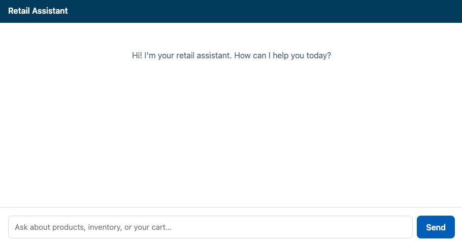
You can now access the retail agent application. From the CDK output values, retrieve the value for AgentObservabilityStack.ChatUrl. Copy and paste this URL into your browser. Log in with your email and password. You should now see the agent interface:

Sample retail agent chat interface showing the ecommerce assistant ready for queries

Figure 2: Sample retail agent user interface

Experiment with the application. Here is an example sequence of queries you can put in:

  • Do you have books on Python?
  • Is this in stock?
  • Put it into my basket.
  • What else can you do for me?

Start Agent Health

Now that you have the infrastructure running, you can start OpenSearch Agent Health locally and connect it to your cloud resources.

The CDK infrastructure deployment created a file cdk-output.json, which contains all relevant configuration values for Agent Health. We’ve already created a file agent-health/agent-health.config.ts that pulls these values dynamically in your environment, so you can start Agent Health without any further configuration.

Open a terminal and start Agent Health by running the following command:

cd ../agent-health && npm install
npx @opensearch-project/agent-health

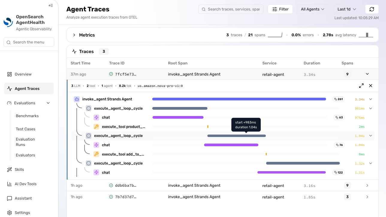
Open http://localhost:4001 in your browser to access Agent Health UI. Choose Agent Traces in the sidebar menu to access your agent’s traces. You should see traces from your previous interactions:

Agent Health Traces view listing agent traces captured from previous interactions

Figure 3: Agent traces. As Agent Health is in active development, this interface might have changed since the time of writing

Expand the trace and explore the information it contains, such as token count and agent trajectory (sequence of messages, reasoning steps, and tool calls).

If you’re unable to access the application or see any traces, verify the following:

  • Check Agent Health logs in your terminal for any errors. Also check whether Agent Health is running on an alternative port, like 4002 instead of 4001.
  • If there are permission errors when accessing traces from OpenSearch, verify that the AWS credentials in your terminal match the principal (user or role) that you specified under the agentHealthReaderArn CDK parameter during cdk deploy. This principal must have ESHttpGet:* IAM permissions. Agent Health uses your current AWS credentials to access the OpenSearch API for querying traces. The OpenSearch API is guarded by both IAM and OpenSearch fine-grained access control.

Create and run a test

Choose Test Cases and New Test Case. Fill out the required fields with the following information:

  • Name: Should add to cart.
  • Initial Prompt: Add some wireless headphones to my cart. Take any that you have in stock.
  • Expected Outcomes: PROD-001 added to cart.

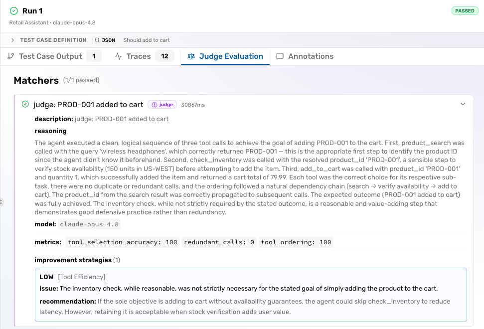
Back in the test cases overview, select the created test case and choose Run Test. In the Configure Run dialog, choose Retail Assistant (production) for Agent, Tool Usage Efficiency for Evaluator, Claude Opus 4.8 for Judge Model, and choose Start Run.

Agent Health now runs the configured initial prompt against the agent. The agent completes the task and sends execution traces to OpenSearch. Agent Health uses an evaluation model to check both agent responses and traces on successful execution, according to the defined expected outcomes. After the test is completed, go through the different tabs to check the test results.

Agent Health evaluation report showing test results across multiple tabs

Figure 4: Agent Health evaluation report

If you’re unable to run the test, check the following:

  • Agent Health automatically creates an Amazon Cognito token for your user upon start, but this token can expire. Restarting Agent Health creates a new token. Verify that both the COGNITO_EMAIL and COGNITO_PASSWORD variables are still set in your terminal environment.

Beyond test cases

After running a single test case, choose Benchmarks in the sidebar menu. With Benchmarks, you can run multiple test cases in parallel and summarize their results. You can compare benchmark runs by choosing Evaluation Runs in the sidebar, where you can analyze trends in pass rate, cost, and duration over time. Lastly, choose Evaluators to define your own evaluation logic beyond the predefined ones.

You can also run Agent Health tests with its command-line interface, which is handy for automation and continuous integration (CI). The equivalent command of running the preceding test is:

npx @opensearch-project/agent-health run -t <TEST_CASE_ID> -a "Retail Assistant" -e system-tool-usage --judge-model claude-opus-4.8 -e system-tool-usage

where TEST_CASE_ID can be retrieved from the browser URL when you visit the Agent Health UI (test case IDs start with tc-).

Agent Health stores all test cases, other configuration, and reports locally on disk in the agent-health/agent-health-data directory.

Cleaning up

To avoid incurring future charges, delete the resources:

cd ../infra && cdk destroy -c agentHealthReaderArn=$AGENT_HEALTH_READER_ARN

Conclusion

In this post, you learned to set up and use OpenSearch Agent Health for production agent observability and evaluations. To discover more features, see the Agent Health documentation pages. You can discuss and request additional features, and get help with setup, through the issues in the GitHub project. For more information, see the observability documentation for Amazon OpenSearch Service, where you can learn about the features available to build observability for both agents and traditional systems using OpenSearch. To investigate issues in production AI agents, see the recent post Unified observability in Amazon OpenSearch Service.


About the authors

Ulli Hinze

Ulli is a Solutions Architect based in Berlin, Germany. He focuses on SaaS, agentic AI, and OpenSearch, and helps customers build and modernize their solutions on AWS. His previous roles included software development, platform engineering, and architecture.

Megha Goyal

Megha is a Senior Software Engineer at AWS OpenSearch. For the past year she has focused on AI agent observability and evaluations, building Agent Health — an open-source developer tool for agents. Previously, she worked on data integrations with Amazon CloudWatch and Amazon Security Lake for the observability and security space. When she’s not building software, she enjoys designing and 3D-printing models at home.

Rekha Thottan

Rekha Thottan

Rekha is a Senior Product Manager Technical on the Amazon OpenSearch Service team.

Measuring and improving search quality with Amazon OpenSearch Service

Post Syndicated from Aruna Govindaraju original https://aws.amazon.com/blogs/big-data/measuring-and-improving-search-quality-with-amazon-opensearch-service/

Search is the front door of many applications, yet most teams struggle to answer a deceptively simple question: “Is my search actually returning relevant results?” Query logs tell you what users typed, not what they saw, what they selected, or why they left. When search feels broken, the culprit is rarely the engine. It’s the lack of deliberate signal collection, measurement, and a feedback loop to act on it.

You can close this gap on Amazon OpenSearch Service using User Behavior Insights (UBI), an open schema standard for capturing search behavior, and Search Relevance Workbench (SRW), a toolkit for measuring and evaluating search quality. Your application generates the UBI-formatted records. Together, UBI and SRW give you a repeatable framework: collect signals, turn them into relevance judgments, and validate every change before it ships.

In this post, we show you how to capture UBI data on an Amazon OpenSearch Service domain and use those signals to evaluate search quality. This is the first post in a two-part series. We build the foundation here, and Part 2 covers automating the workflow end to end.

The challenge: You can’t improve what you can’t measure

Consider a shopper searching for “handbag” on an ecommerce site. The catalog has 16 products (tote bags, duffel bags, laptop bags), but every title only says “bag.” The search returns zero results. Most shoppers leave. A patient one retries with “bag” and finds what they were looking for.

Your server log recorded that first query as a clean sub-second response: no error, no alert, no signal. What it missed entirely was a customer with purchase intent. That customer hit a vocabulary gap between how they search and how you write your catalog. Zoom out and apply this lens to misspelled queries, poor handling of long-tail searches, and abandoned sessions. The blind spot is larger than you think.

There’s a second problem: click signals are position biased. Users select the first result far more than the fifth, regardless of relevance, so raw click counts reflect where results appeared, not whether they deserved to be there. Any judgment derived from clicks must correct for this bias. We return to it when generating judgments.

Capturing behavioral data with UBI

UBI defines two indices. The ubi_queries index holds one record per executed query: the text the user typed, the full query that ran (filters and facets included), and the IDs of the documents returned. The ubi_events index holds every subsequent user action: impressions, hovers, clicks, add-to-carts, each stamped with the result position and the product’s business identifier (object_id). A shared query_id links every event back to the query that triggered it. Two additional identifiers complete the picture: client_id tracks the browser across visits, and session_id scopes events to a single visit.

A query record captures what the user asked and which document IDs the engine returned, including zero-result cases like the handbag search, which appears as a record with an empty result list. Here’s the shopper’s follow-up search for “bag”:

{
  "query_id": "1bf736d4-d673-4763-9193-4bc8a2282115",
  "client_id": "9a9968ac-664b-42d7-9a9e-96f412b5ab49",
  "user_query": "bag",
  "query": "{"multi_match": {"query": "bag", "fields": ["title", "description", "category", "brand"]}}",
  "query_response_hit_ids": [
    "3760170840499",
    "8400000000042"
  ],
  "timestamp": "2026-07-23T07:53:35.264Z",
  "application": "retail-shop"
}

The UBI queries schema reference documents the complete query schema, including the mandatory attributes.

The event record captures what the user did next. For each result rendered, emit an impression event. When the user selects a result, emit a click event. Here is the impression event for the first result of the bag search:

{
  "action_name": "impression",
  "query_id": "1bf736d4-d673-4763-9193-4bc8a2282115",
  "client_id": "9a9968ac-664b-42d7-9a9e-96f412b5ab49",
  "session_id": "0f2e6f2a-8f4e-4f60-9f6e-2a1b3c4d5e6f",
  "user_query": "bag",
  "timestamp": "2026-07-23T07:53:41.112Z",
  "event_attributes": {
    "position": {
      "ordinal": 1
    },
    "object": {
      "object_id": "3760170840499",
      "object_id_field": "object_id"
    }
  }
}

event_attributes also accepts custom fields of your own alongside the standard position and object structures. The action_name attribute is critical: The judgment model you use later consumes only impression and click events. Treat a paginated results page as the same logical query: reuse the query_id and record absolute positions. The UBI events schema reference documents the complete event schema.

Collecting UBI data on Amazon OpenSearch Service

Behavioral data (what results ranked, what users saw, what they selected) exists only in the application layer. Your application owns the records, and Amazon OpenSearch Ingestion (OSI), a fully managed, serverless data collector powered by Data Prepper, provides the managed delivery path. Your application sends the records as SigV4-signed HTTP POST requests to the OSI pipeline endpoints. Route browser events through your backend for signing. One thing to understand before you write any code: Your application generates and owns the query_id attribute. The application creates the ID when it runs a search and stamps it on every subsequent event the user produces, until the user issues a new search or the session ends.

Prerequisites

To follow along, you need an Amazon OpenSearch Service domain running OpenSearch 3.5 or later with the OpenSearch UI application, permissions to create OpenSearch Ingestion pipelines with an AWS Identity and Access Management (IAM) pipeline role, and a search application you can instrument to emit behavioral records.

Create the UBI indices

Before you start collecting user metrics, you need the two indices in place with the right mappings. Field types matter here: query_id as keyword supports exact joins between queries and events, timestamp as date supports time-range queries, and event_attributes as dynamic means you can extend events with custom fields without schema changes.

Create ubi_queries first in Dev Tools. It holds the query-side records. We abbreviated the mappings here. Refer to the published queries-mapping.json file for the complete version:

PUT ubi_queries
{
  "mappings": {
    "properties": {
      "query_id": { "type": "keyword" },
      "client_id": { "type": "keyword" },
      "user_query": { "type": "keyword" },
      "query_response_hit_ids": { "type": "keyword" },
      "timestamp": {
        "type": "date",
        "format": "strict_date_time"
      },
      "application": { "type": "keyword" }
    }
  }
}

Then create ubi_events. It holds every user action that follows (refer to the full events-mapping.json file):

PUT ubi_events
{
  "mappings": {
    "properties": {
      "query_id": { "type": "keyword", "ignore_above": 100 },
      "action_name": { "type": "keyword", "ignore_above": 100 },
      "client_id": { "type": "keyword", "ignore_above": 100 },
      "session_id": { "type": "keyword", "ignore_above": 100 },
      "user_query": { "type": "keyword" },
      "timestamp": {
        "type": "date",
        "format": "strict_date_time"
      },
      "event_attributes": {
        "dynamic": true,
        "properties": {
          "position": {
            "properties": {
              "ordinal": { "type": "integer" }
            }
          },
          "object": {
            "properties": {
              "object_id": { "type": "keyword" },
              "object_id_field": { "type": "keyword" }
            }
          }
        }
      }
    }
  }
}

With both indices created, the next step is routing data into them. You can deliver UBI data to your domain in several ways. This post uses OSI pipelines, shown end to end in the diagram that follows the setup.

Set up the OSI pipelines

Create two OSI pipelines: one for queries and another for events. Each pipeline exposes an HTTP source endpoint that your application writes to (shown on each pipeline’s console page) and sinks data to the corresponding index. The following configuration defines the events pipeline:

version: '2'
ubi-events:
  source:
    http:
      path: /ubi/events
      max_request_length: 10mb
  processor:
    - date:
        from_time_received: true
  sink:
    - opensearch:
        hosts: ["https://<domain-endpoint>"]
        aws:
          serverless: false
          region: <region>
          sts_role_arn: <pipeline-role-arn>
        index_type: custom
        index: ubi_events
    - s3:
        aws:
          region: <region>
          sts_role_arn: <pipeline-role-arn>
        object_key:
          path_prefix: 'ubi_events/%{yyyy}/%{MM}/%{dd}'
        bucket: <bucket-name>
        threshold:
          maximum_size: 50mb
          event_collect_timeout: 60s
        codec:
          ndjson:

Note: the queries pipeline follows the same pattern, with /ubi/queries as the path and ubi_queries as the sink index and S3 prefix. Create the pipeline role yourself or let OpenSearch Ingestion create it. If your domain uses fine-grained access control, also map the pipeline role to a backend role so the domain accepts the pipeline’s writes. Refer to the tutorial Collecting UBI-formatted data in Amazon OpenSearch Service for detailed steps.

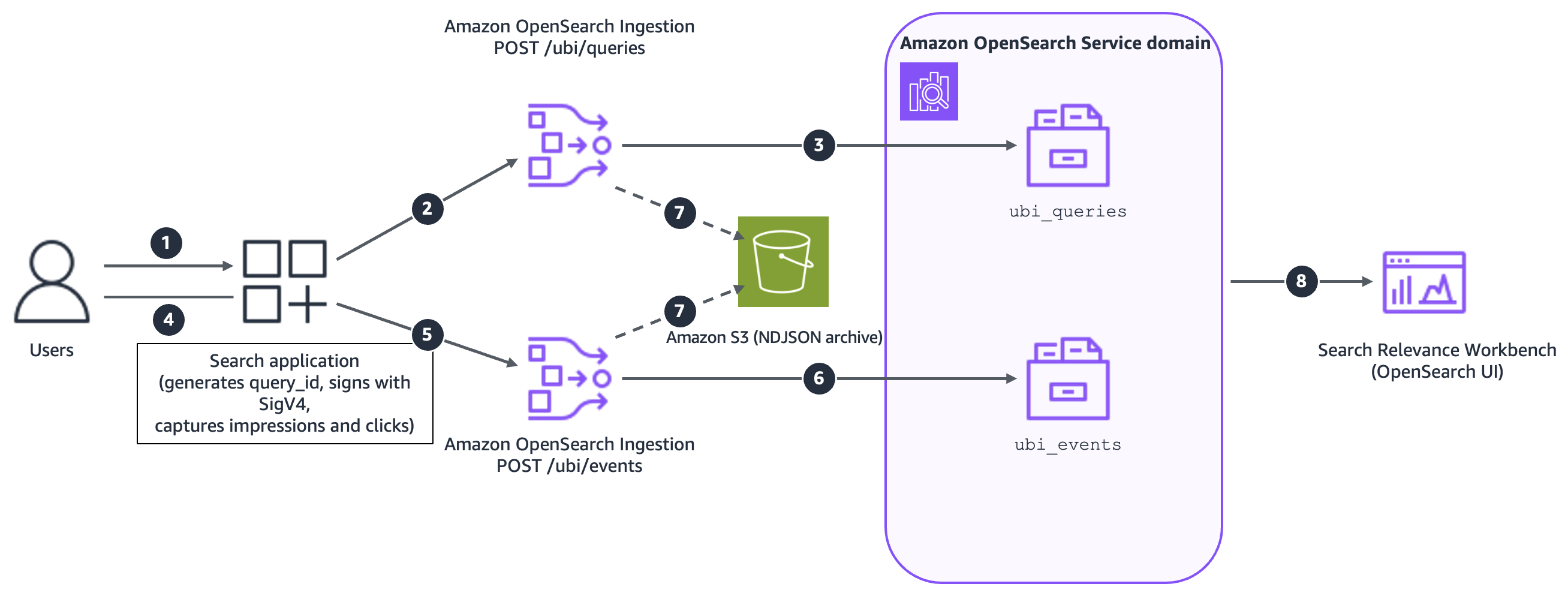
With the pipelines running, your application can start sending data. The following diagram illustrates the end-to-end flow:

UBI collection flow from the search application through OpenSearch Ingestion into the ubi_queries and ubi_events indices

Figure 1: The UBI collection pattern on Amazon OpenSearch Service

The workflow consists of the following steps:

  1. Users interact with your search application.
  2. The application sends signed query records to the OSI HTTP endpoint.
  3. OSI writes queries to the ubi_queries index.
  4. Users interact with the results, viewing and selecting documents.
  5. The application sends signed event records, carrying the same query_id, to the OSI HTTP endpoint.
  6. OSI writes events to the ubi_events index.
  7. Optionally, both pipelines archive records to Amazon Simple Storage Service (Amazon S3).
  8. Search Relevance Workbench (OpenSearch UI) works with the collected data in the ubi_queries and ubi_events indices.

Note: if you’re already collecting site analytics through an existing third-party tool, you don’t need to replace it. Map your search-related events (queries, clicks, and conversions) into the UBI schema and store them in OpenSearch. That’s enough to unlock the out-of-the-box evaluation framework, implicit judgment generation, and the full SRW metrics pipeline, without defining a single custom metric from scratch.

Visualize the data collected

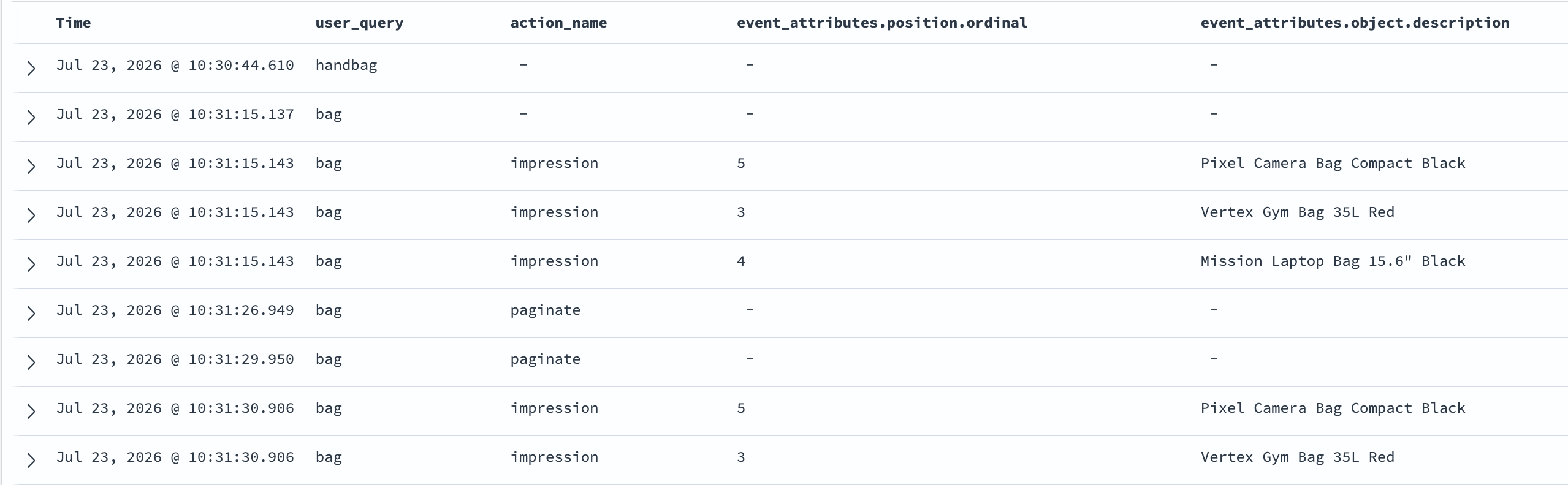
After the UBI behavior metrics start to trickle in, you can review the data in the Discover tab on the OpenSearch UI dashboard. Filtering ubi_queries for empty result lists ranks your vocabulary gaps. You can also visualize the data collected through the sample User Behavior Insights (UBI) dashboards in OpenSearch.

OpenSearch Discover view of UBI records for the zero-result handbag query and the follow-up bag query

Figure 2: UBI records in Discover, showing the zero-result handbag query and the follow-up bag query with its impressions and pagination events

With data flowing into your indices, keep these things in mind as you scale to production:

  • Keep telemetry off the search critical path – Queue records and forward them asynchronously. Losing a fraction of behavioral data is statistically harmless. Blocking users isn’t.
  • Manage volume deliberately – Batch impression events, and if you sample, sample whole queries rather than individual events to preserve the click-through ratios that drive judgments.
  • Isolate analytical load for larger deployments – Route pipelines to a separate analysis domain with the same engine version, mappings, and analyzers as production. This keeps behavioral writes from touching live search latency.
  • Plan for retention and integrity – Register the UBI mappings as an index template and apply an Index State Management (ISM) retention policy as your indices grow. You should validate and rate-limit the event write path, and cover query text and client identifiers with your data retention policy.

Evaluating search quality with Search Relevance Workbench

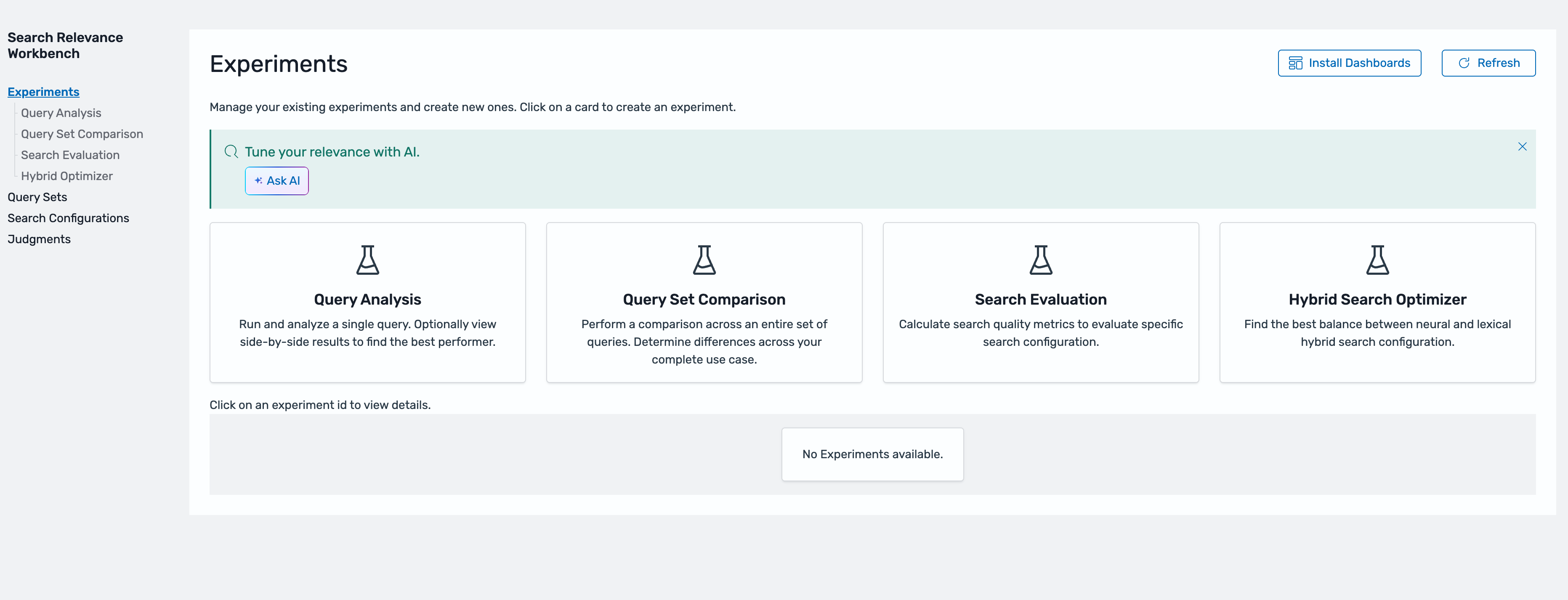
With ubi_queries and ubi_events collecting data, you now have the signals needed to evaluate search quality. Search Relevance Workbench, generally available in the OpenSearch UI from Amazon OpenSearch Service 3.5, turns those signals into structured experiments: comparing query configurations, scoring results against relevance judgments, and surfacing metrics that guide iterative tuning.

The Search Relevance Workbench home screen in the OpenSearch UI

Figure 3: Search Relevance Workbench in the OpenSearch UI

SRW experiments rely on three components. You set them up once, then reuse them across every experiment you run: a query set (the fixed queries you evaluate against), search configurations (the query structures you want to compare), and a judgment list (the relevance ground truth). The following sections walk through each one.

Step 1: Create a query set

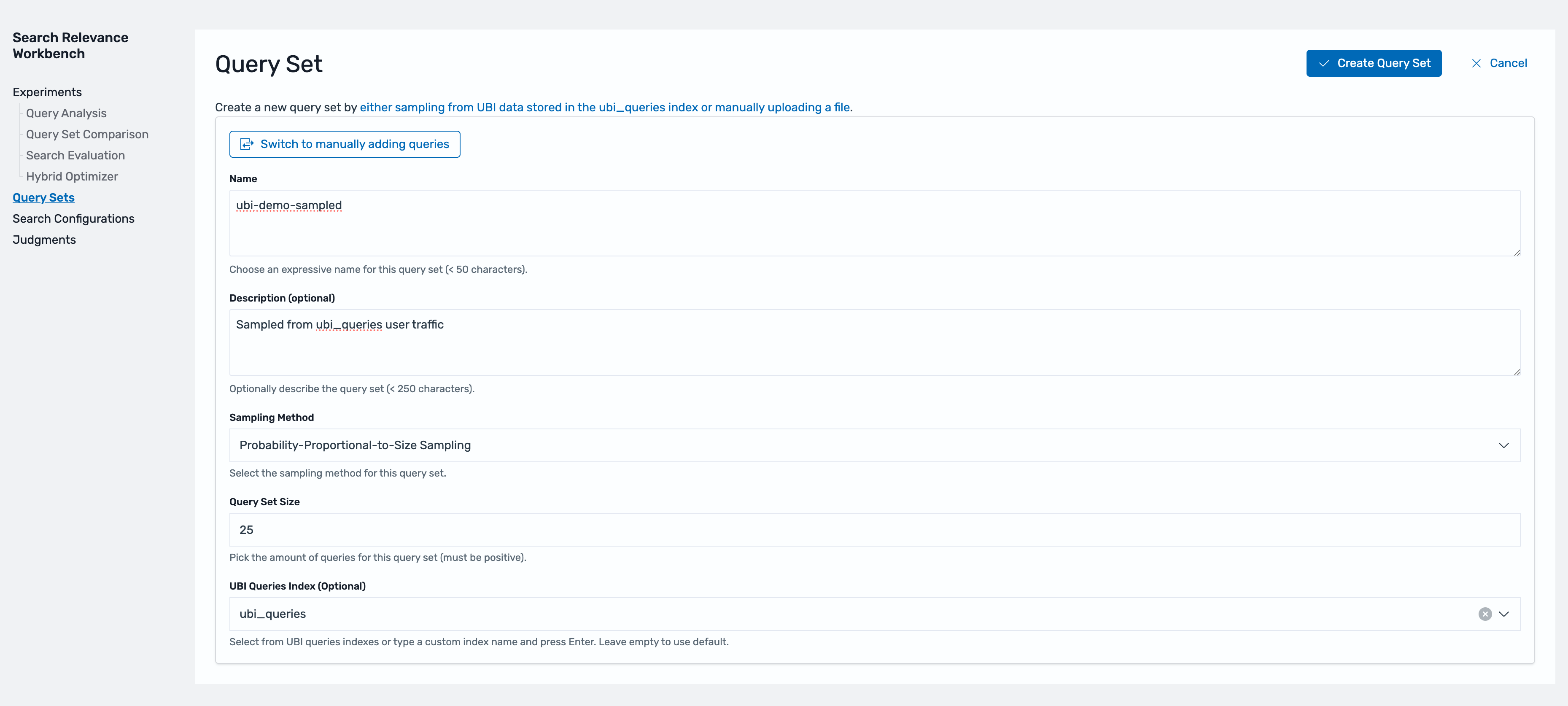
A query set is the fixed collection of queries you evaluate against. Keeping it fixed makes results comparable across experiments. Effective query sets reflect real traffic, not intuition. You can seed one from your top queries, a random sample, or a hand-picked mix that includes long-tail and low-performing queries. Alternatively, SRW can sample directly from ubi_queries using Probability-Proportional-to-Size (PPS) sampling, which selects queries in proportion to how often users issue them. This approach represents frequent queries like “bag”, so your metrics reflect search quality as users experience it.

Query set creation screen sampling queries from real traffic in the ubi_queries index

Figure 4: Creating a query set sampled from real traffic in ubi_queries

Step 2: Define search configurations

A search configuration defines how a search executes: the index, the query structure, and a %SearchText% placeholder that SRW replaces with each query in your set. Creating two configurations and running them against the same query set and judgment list is how you validate a change before any user sees it.

As an example, here we define two configurations: a baseline multi_match query (retail_query) and a variant that boosts title matches (retail_boosted_query), so we can measure whether the boost actually helps ranking.

retail_query retail_boosted_query
{
  "query": {
    "multi_match": {
      "query": "%SearchText%",
      "fields": [
        "title",
        "description",
        "category",
        "brand"
      ]
    }
  }
}
{
  "query": {
    "multi_match": {
      "query": "%SearchText%",
      "fields": [
        "title^2",
        "description",
        "category",
        "brand"
      ]
    }
  }
}

Configurations go beyond query variants: a candidate can be an entirely different retrieval strategy, like hybrid search combining keyword and neural retrieval. You can use judgments to rate query-document pairs independently of your retrieval approach. You can test a semantic or hybrid approach offline against your existing traffic before shipping it.

Step 3: Create the judgment list

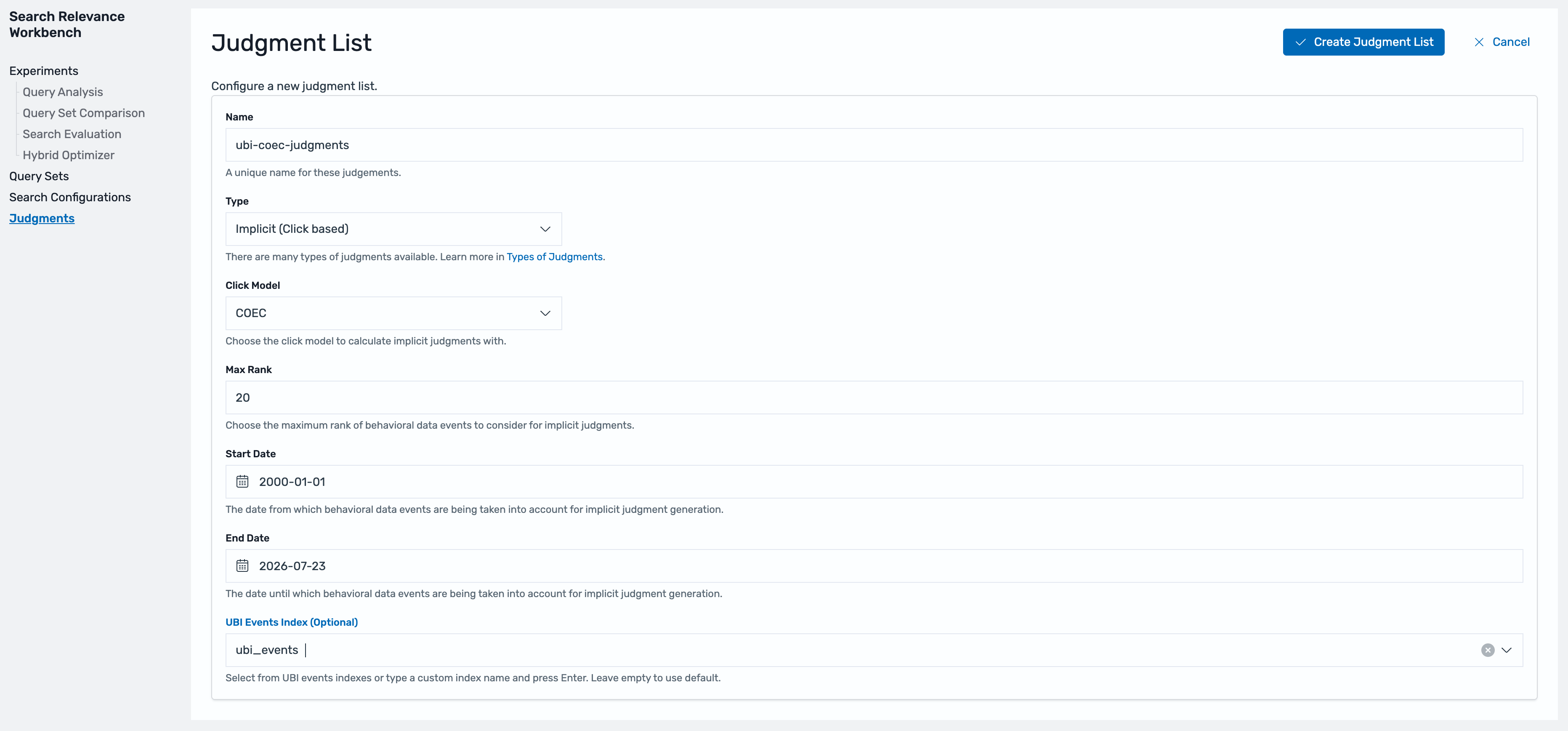
A judgment is a relevance rating for a query-document pair: the ground truth that quality metrics measure against. You can create judgments that are explicit (from stakeholders or a large language model acting as judge), imported, or implicit (derived from behavior). Here we use implicit judgments derived from UBI selection behavior, scored using the Clicks Over Expected Clicks (COEC) model. The COEC model helps correct position bias by comparing each document’s actual click rate against the expected rate for its rank position. Documents that outperform their position score as relevant. Those that users select because they ranked first score near average.

Judgment list creation screen with the Implicit click-based type and COEC click model selected

Figure 5: Creating an implicit judgment list with the Implicit (Click based) type and the COEC click model

Three things to get right before you run experiments:

  1. object_id in your events must match the document _id from your product catalog. The search configurations you define return this _id, which lets SRW join judgments to results.
  2. Implicit judgments are statistical. They need volume and query coverage. As a working rule of thumb, aim for hundreds to thousands of real sessions per query to separate signal from noise.
  3. Max Rank controls how deep in the result list events count. If users paginate, set it beyond a single page. We use 20 here.

Step 4: Run experiments

This post uses three SRW capabilities: Query Analysis, Query Set Comparison, and Search Evaluation. Query Analysis is a quick eyeball check: compare two configurations side by side for a specific query to see exactly what changed and why the metrics moved. The other two answer harder questions with numbers: how good a configuration is, and how two configurations compare against real relevance signals.

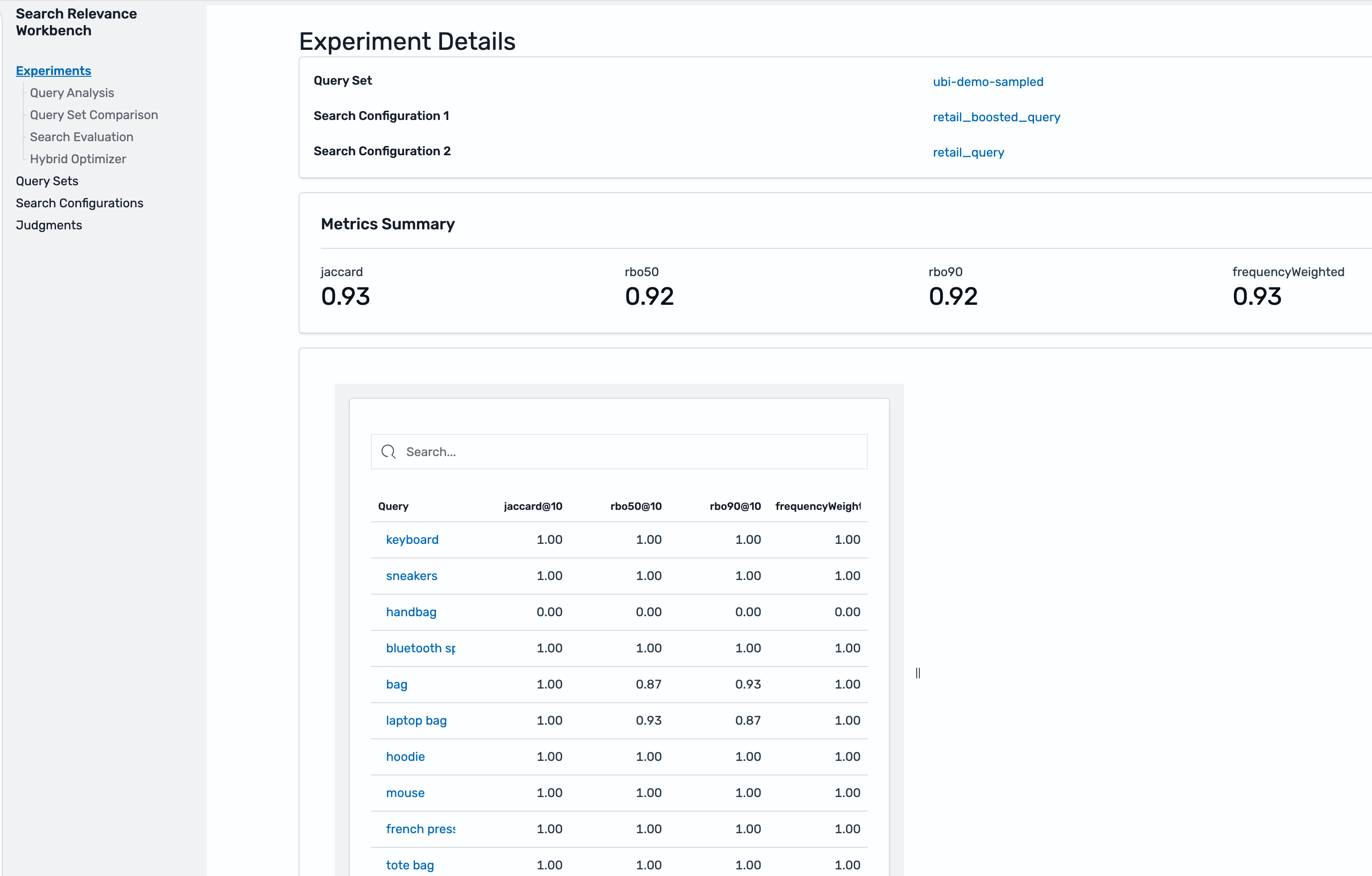
Query Set Comparison (also called pairwise comparison) takes two configurations and computes ranking similarity. Jaccard overlap measures how much the two result lists share, while Rank-Biased Overlap (RBO) weights agreement at the top of the list more heavily. Near-identical scores mean the change will barely register with users. Low overlap means a real ranking shift worth reviewing carefully before shipping. In this run, the two configurations score 0.93 Jaccard and 0.92 RBO, a modest but real shift. SRW cannot score zero-result queries like “handbag”: They show zero similarity in a comparison and Failed in an evaluation, a signal they need a different fix than ranking adjustments.

Query Set Comparison results showing Jaccard and Rank-Biased Overlap scores for the two configurations

Figure 6: Query Set Comparison showing Jaccard and Rank-Biased Overlap between the two configurations

Search Evaluation (also called pointwise evaluation) scores one configuration against your query set and judgment list across four metrics, each computed over the top k results (k=10 by default):

Metric What it measures What it tells you
Coverage@k Proportion of returned documents that have judgments How much to trust the other three metrics. Low Coverage means many results were never judged
Precision@k Fraction of the top k results that are relevant How many irrelevant results appear on the first page
MAP@k (Mean Average Precision) Precision averaged across ranks, rewarding relevant documents placed early Whether relevant results appear early, even when Precision ties
NDCG@k (Normalized Discounted Cumulative Gain) Graded judgment values, discounted by position (rank 1 counts more than rank 9) Whether the best results appear first. The primary comparison metric

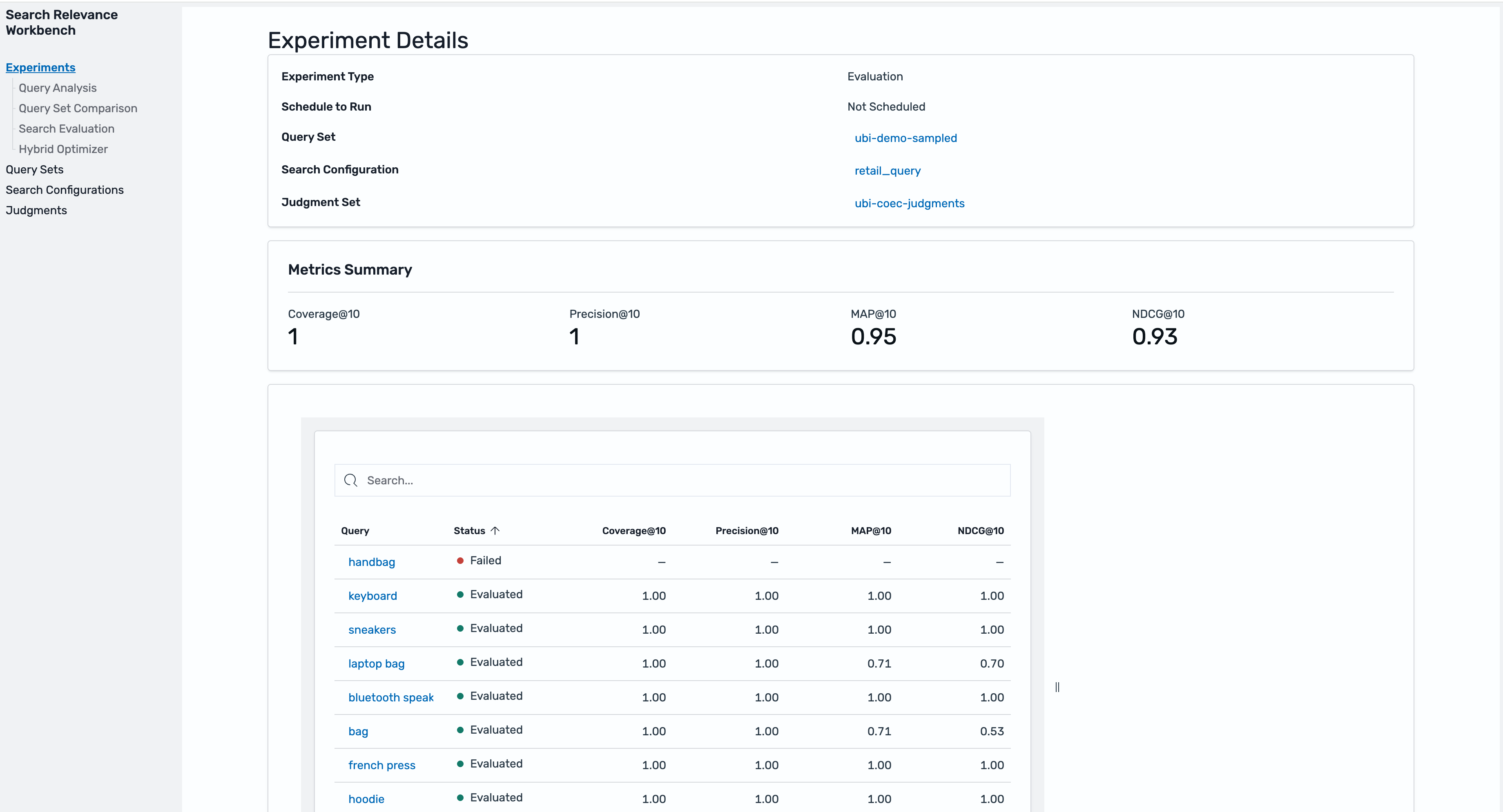
Each pointwise experiment evaluates one configuration. To compare candidates, run one experiment per configuration and compare the results. In this run, the baseline (retail_query) scores Coverage@10 of 1.0, Precision@10 of 1.0, MAP@10 of 0.95, and NDCG@10 of 0.93, with the zero-result “handbag” query showing as Failed in the per-query detail.

Search evaluation results showing Coverage, Precision, MAP, and NDCG at 10 with per-query detail

Figure 7: Search evaluation results for one configuration: Coverage, Precision, MAP, and NDCG at 10, with per-query detail

From measurement to improvement

The preceding experiments are the harness. The following are common levers to test with it. Express each as a new search configuration, evaluate it against the same query set and judgment list, and adopt it only if the metrics move:

  • Synonyms – One option for addressing known vocabulary gaps is to build synonyms. A search-time synonym token filter treats “handbag” and “bag” as equivalent, and with Amazon OpenSearch Service, you can hot deploy custom synonym packages without reindexing.
  • Field weights – Adjust the fields and boosts in a multi_match query, like the title^2 variant tested earlier.
  • Semantic retrieval – A hybrid query combines keyword and neural scores, addressing vocabulary mismatch as a class rather than term by term. Judgments evaluate it offline exactly like a lexical candidate.
  • Reranking – A rerank processor in a search pipeline reorders the top results using a cross-encoder model.

Clean up

To avoid future charges, delete the resources you created for this walkthrough:

  • Delete the two OpenSearch Ingestion pipelines. To reuse them later, stop them instead. A stopped pipeline keeps its configuration and incurs no OpenSearch Compute Unit (OCU) hour charges.
  • If you configured the optional Amazon S3 archive, delete the archived objects (or the bucket).
  • If you keep the domain, optionally delete the ubi_queries and ubi_events indices and the query sets, judgment lists, and experiments you created. These live on the domain and incur no separate charges.
  • If you created the domain specifically for this post, delete it to remove everything, including the resources in the previous step. Deleting a domain is irreversible. Don’t delete a domain that serves other workloads.

Conclusion

UBI collects the evidence, COEC turns it into judgments, and SRW experiments deliver the verdict: Coverage, Precision, MAP, and NDCG in place of guesswork. Ship the winning configuration, keep collecting, and the next round of judgments shows whether the improvement holds with real behavior. Where there used to be an opinion, there is now a number.

Everything here follows a repeatable pattern, and repeatable patterns lend themselves to automation. Part 2 walks through the Search Relevance Agent, available through the AI Assistant chat (the Ask AI button) in the OpenSearch UI. The agent analyzes your UBI signals, generates tuning hypotheses, and validates them offline before recommending changes. The pipeline you built in this post is the foundation. Stay tuned for Part 2.

To go deeper on the evaluation features, refer to the Search Relevance Workbench documentation.


About the authors

Aruna Govindaraju

Aruna Govindaraju

Aruna is an Amazon OpenSearch Specialist Solutions Architect and has worked with many commercial and open source search engines. She is passionate about search, relevancy, and user experience. Her expertise with correlating end-user signals with search engine behavior has helped many customers improve their search experience.

Sean Bjurstrom

Sean Bjurstrom

Sean is an Enterprise Support Lead in ISV accounts at Amazon Web Services, where he specializes in Analytics technologies and draws on his background in consulting to support customers on their analytics and cloud journeys. Sean is passionate about helping businesses harness the power of data to drive innovation and growth. Outside of work, he enjoys running and has participated in several marathons.

Utkarsh Agarwal

Utkarsh Agarwal

Utkarsh is a Cloud Support Engineer in the Support Engineering team at AWS. He provides guidance and technical assistance to customers, helping them build scalable, highly available, and secure solutions in the AWS Cloud. In his free time, he enjoys watching movies, TV series, and, of course, cricket! Lately, he has also been attempting to master foosball.

Querying raw log data using SQL and PPL with the optimized engine in Amazon OpenSearch Service

Post Syndicated from Kaushik Krishnan original https://aws.amazon.com/blogs/big-data/querying-raw-log-data-using-sql-and-ppl-with-the-optimized-engine-in-amazon-opensearch-service/

In this post, you learn how to run fast analytical queries directly against raw log and trace data in Amazon OpenSearch Service using PPL and SQL.

Amazon OpenSearch Service is a fully managed service that helps you deploy, scale, and operate OpenSearch, the open source suite for search, analytics, and observability in the AWS Cloud. OpenSearch Service powers search and real-time analytics workloads, from lexical and hybrid search to log analytics and observability. This post focuses on log analytics, and on a practical question: how much analytical work can you do directly against raw log and trace data, without moving it or reshaping it first?

The new optimized engine in OpenSearch Service answers that question: you can point Piped Processing Language (PPL) and Structured Query Language (SQL) queries at raw log and trace data. The engine returns aggregations, filters, and scans over billions of events on the data exactly as you ingested it. In this post, you follow a single incident investigation, one query at a time. You see how the engine answers each new question, from multi-dimensional breakdowns and latency distributions to error rates and fleet sizing. No precomputed structure sits behind the results.

How the optimized engine queries raw data

The optimized engine stores data in the columnar Apache Parquet format and runs queries through Apache DataFusion, a vectorized execution engine, with Apache Calcite planning each query. Because the engine stores data in columns, an analytical query reads only the columns it touches and processes their values in batches, instead of reading each matching document in full. Alongside the columnar format, the engine also keeps an inverted index on the same data, so the query planner routes each operation to the path that serves it best: the columnar engine for aggregations and analytical scans, and the inverted index for selective search and filtering.

You ingest your logs and traces through the same Bulk API and clients you use today, and you write PPL or SQL against them as they land.

An investigation, one query at a time

The following walkthrough traces a common observability use case, root-cause analysis during a live incident, from the perspective of a site reliability engineer (SRE). The engineer notices elevated latency and a handful of error alerts, with nothing that points to a clear cause. No existing dashboard covers this particular shape of problem, so the engineer opens Amazon OpenSearch Service and starts asking questions of the raw trace data, letting each answer decide the next one. PPL suits this work well. Each command transforms the data and passes it to the next, so the engineer reads a query left to right the same way they think through the investigation.

The walkthrough uses generated OpenTelemetry (OTEL) data from a synthetic load generator, at billion-document scale. The focus is the query capability, that is, what the engineer can express and retrieve directly from raw spans, rather than the specific values in each result.

Step 1: Assess the scope

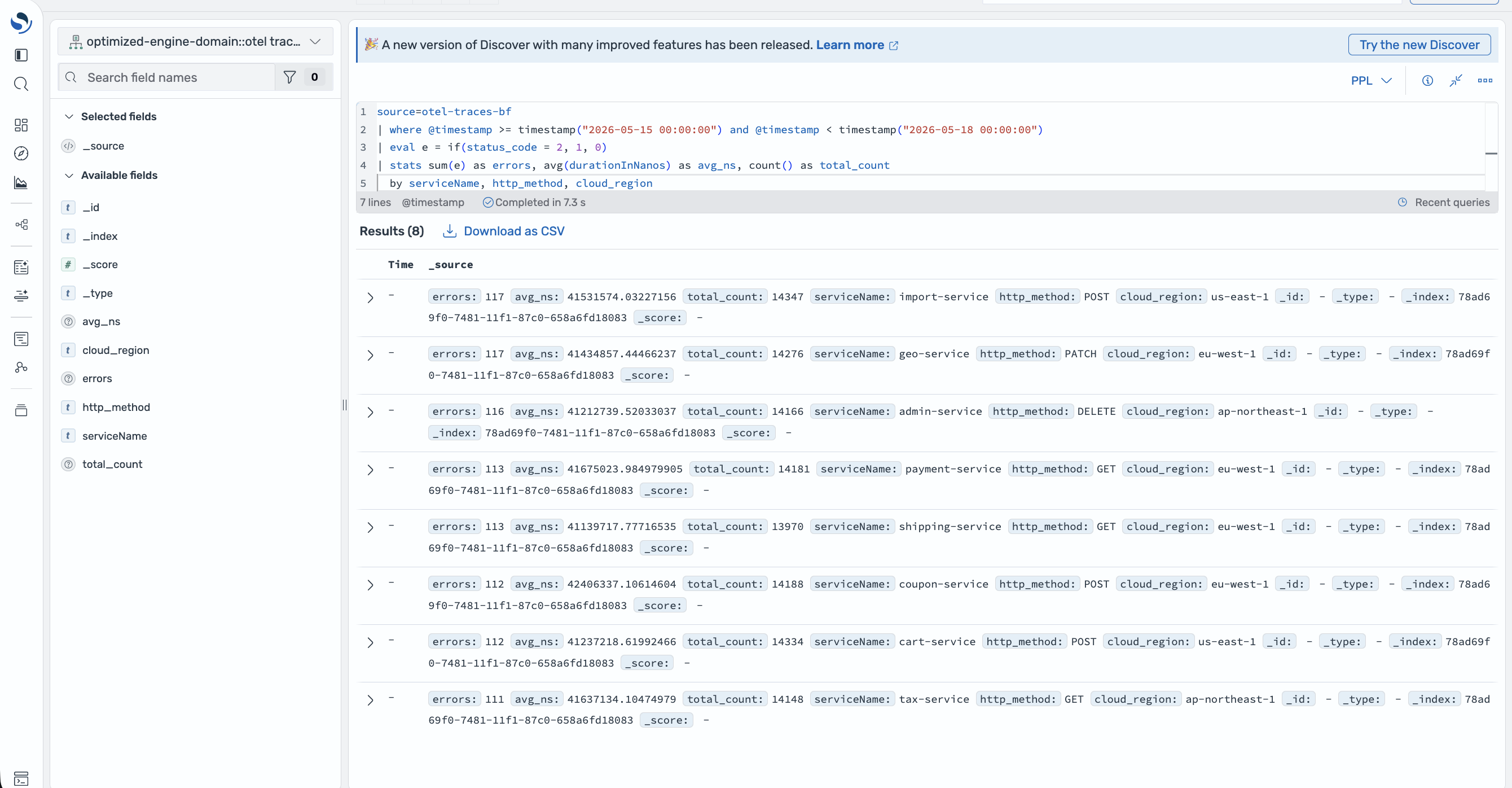
The first question in any investigation is how widespread the signal is. The engineer breaks errors down across service, HTTP method, and cloud Region in a single pass over roughly 1.1 billion spans.

source=otel-traces
| where @timestamp >= timestamp("2026-05-15 00:00:00") and @timestamp < timestamp("2026-05-18 00:00:00")
| eval e = if(status_code = 2, 1, 0)
| stats sum(e) as errors, avg(durationInNanos) as avg_ns, count() as total_count
  by serviceName, http_method, cloud_region
| sort - errors
| head 8

In plain terms, this query answers the engineer’s first question: where are the failures happening? It counts the error spans and breaks them down by service, HTTP method, and AWS Region in a single pass. Rather than guessing which service to open first, the engineer gets a ranked list of the hardest-hit combinations to investigate.

errors total_count avg_ns serviceName http_method cloud_region
730 112,436 41,246,806 export-service GET us-west-2
722 111,215 41,000,227 catalog-service PUT eu-central-1
704 112,051 41,295,539 image-service PATCH us-west-2
612 93,214 41,451,145 healthcheck-service PUT us-east-1
609 94,314 41,418,897 auth-service POST us-east-1
609 94,414 41,447,444 email-service PATCH ap-northeast-1
593 89,726 41,047,114 payment-service PUT eu-central-1
581 89,854 41,195,643 file-service PUT ap-northeast-1

The errors spread across services, methods, and Regions, which points to a systemic pattern rather than a single misbehaving service.

Step 2: Check whether one host concentrates the failures

The spread could still reflect one saturated node or a fleet-wide condition. To tell the two apart, the engineer groups failures by exception type, service, and host across the entire index, with no time filter to narrow the scan.

source=otel-traces
| where isnotnull(exception_type)
| stats count() as total_count by exception_type, serviceName, host_name
| sort - total_count
| head 8
total_count exception_type serviceName host_name
6 DeadlockDetectedException notification-service ip-10-0-16-34
6 IllegalStateException api-gateway ip-10-0-180-234
6 FileNotFoundException cart-service ip-10-0-90-162
6 ConnectionRefusedException feature-flag-service ip-10-0-8-123
5 TimeoutException auth-service ip-10-0-97-78
5 ConcurrentModificationException order-service ip-10-0-165-15
5 TimeoutException coupon-service ip-10-0-158-25

In this sample the counts are low and every row lands on a different host, so no single node stands out. This points to a fleet-wide pattern rather than one bad machine. On production data the same query makes the distinction directly: a code-level bug shows up across many hosts, whereas a single failing node concentrates its errors on one host_name.

Step 3: Quantify the latency distribution per service

Next, the engineer pulls a latency profile for each service. This includes count, average, minimum, and maximum duration, to see how each one behaves and how wide the spread runs.

source=otel-traces
| where @timestamp >= timestamp("2026-05-15 00:00:00") and @timestamp < timestamp("2026-05-18 00:00:00")
| stats count() as total_count, avg(durationInNanos) as avg_ns, min(durationInNanos) as min_ns, max(durationInNanos) as max_ns
  by serviceName
| sort - total_count
| head 8
serviceName total_count avg (ns) min (ns) max (ns)
event-bus 11,087,263 41,249,552 26,113 9,304,132,159
scheduler-service 9,175,964 41,251,927 21,919 13,432,040,933
cdn-service 9,173,572 41,225,385 23,468 13,768,293,306
ml-inference 9,036,753 41,289,101 40,410 14,625,084,517
compliance-service 8,274,635 41,294,694 41,915 7,462,983,016
metrics-collector 7,804,234 41,334,728 16,535 23,228,217,669
notification-service 7,688,714 41,204,635 51,562 8,695,311,374
image-service 7,674,406 41,248,069 47,473 15,350,500,299

This gives the engineer a latency fingerprint for each service: the averages sit near 41 milliseconds. But the multi-second maxima reveal a long tail consistent with requests queuing behind a slow dependency.

Step 4: Measure the error rate per service

To track a service-level objective, the engineer computes the error rate (errors against total requests) per service. The query uses an inline conditional, followed by a grouped sum and count, and a final division to produce the error rate.

source=otel-traces
| eval is_err = if(status_code = 2, 1, 0)
| stats sum(is_err) as errors, count() as total_count by serviceName
| eval error_pct = round(100.0 * errors / total_count, 2)
| sort - error_pct
| head 8
errors total_count error_pct serviceName
699,358 22,415,308 3.12 payment-service
647,811 26,880,140 2.41 checkout-service
562,811 30,096,860 1.87 auth-service
316,192 24,510,990 1.29 cart-service
288,314 30,671,704 0.94 order-service
202,612 28,140,552 0.72 search-service
186,012 33,820,415 0.55 catalog-service
134,722 35,453,247 0.38 image-service

The engineer defines the error-rate metric in the query itself, and the engine computes it across the full index. The busiest paths, payment and checkout, run near 3 percent, whereas some services stay below 1 percent.

Step 5: Size the fleet footprint with SQL

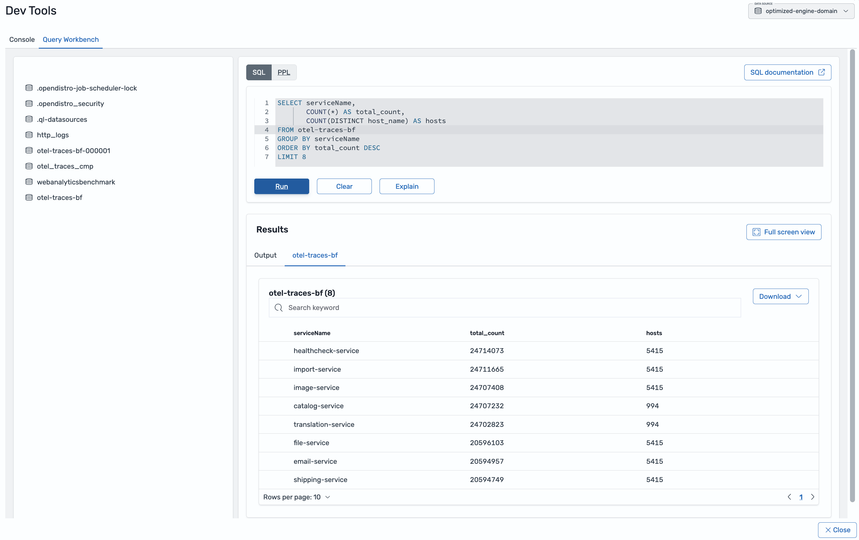
Finally, the engineer sizes how much of the fleet each service spans, a capacity and impact question, and switches from PPL to SQL to express it.

SELECT serviceName,
       COUNT(*) AS total_count,
       COUNT(DISTINCT host_name) AS hosts
FROM otel-traces
GROUP BY serviceName
ORDER BY total_count DESC
LIMIT 8
serviceName total_count hosts
ml-inference 35,481,688 2,535
image-service 35,453,247 2,491
email-service 35,443,569 2,517
shipping-service 30,700,372 2,438
translation-service 30,490,570 2,502
auth-service 30,096,860 2,466
chat-service 25,564,111 2,449
recommendation-service 25,366,844 2,483

The query runs a COUNT(DISTINCT) over a high-cardinality field at billion-row scale, and switching languages mid-investigation costs the engineer nothing more than writing SQL instead of PPL. The host counts cluster in the approximately 2,400–2,540 range, so each service runs across a broad slice of the fleet. That confirms the earlier finding: the errors reflect a fleet-wide pattern, not a single node.

The engineer asked five questions and ran five queries, and each answer shaped the next. The optimized engine served every query directly from raw trace data, across both PPL and SQL, without a rollup table or precomputed summary behind any result.

Run these queries where you already work

You don’t need a separate tool to run the queries in this walkthrough.

Figure 1: Investigation queries and results grid in Query Workbench

Query Workbench in OpenSearch Dashboards UI gives you a dedicated editor for PPL and SQL. You write a query, run it, and read the results in a grid, using the same queries shown throughout this post. When you want to move from a written query to interactive exploration, Discover runs the same PPL and SQL against your indexes. In Discover, you can filter, expand fields, and drill into individual documents without leaving the page. The same query language works in both places, so you can start an investigation in Discover and carry it into Query Workbench, or the reverse, without rewriting anything.

Figure 2: PPL query and field list in Discover

Keep all your data and query it as it is

Querying raw data directly only helps if you can afford to keep the raw data. The optimized engine compresses observability data up to 70 percent more efficiently than the default General Purpose engine. That compression turns “keep everything and query it directly” into a practical default. You retain full-fidelity data for the questions you cannot predict in advance. You also pay less to store it than you would to store the raw JSON.

Get started

To try the optimized engine, create an Amazon OpenSearch Service domain running OpenSearch 3.5 or later. Then select the Observability use case during setup, which provisions the domain with the optimized engine.

To learn more about configuring and using the optimized engine, see Optimized for Log Analytics in the Amazon OpenSearch Service documentation. For an overview of the service, visit Amazon OpenSearch Service Log Analytics.

For more information, see the blog post Run log analytics for a fraction of the cost with the new engine for Amazon OpenSearch Service.

Give it a try and send feedback to AWS re:Post for Amazon OpenSearch Service or through your usual AWS Support contacts.


About the authors

Kaushik Krishnan

Kaushik is a Technical Account Manager at Amazon Web Services with a focus on Amazon OpenSearch Service. He is based in the Washington, D.C. area and specializes in troubleshooting critical operational and performance issues as well as conducting architectural reviews of OpenSearch clusters for customers. Outside of work, he enjoys playing soccer and is an avid traveler.

Luis Tiani

Luis is a Sr Solutions Architect at AWS. He specializes in data and analytics topics, with extensive focus on Amazon OpenSearch Service for search, log analytics, and vector environments. Tiani has helped numerous customers across financial services, DNB, SMB, and enterprise segments in their OpenSearch adoption journey, reviewing use cases and providing architecture design and cluster sizing guidance.

Jagadish Kumar

Jagadish is a Senior Solutions Architect at Amazon Web Services, focused on OpenSearch and analytics workloads.

How Zepto powers sub-second search using OpenSearch Service OR2 instances

Post Syndicated from Kayalvizhi Kandasamy original https://aws.amazon.com/blogs/big-data/how-zepto-powers-sub-second-search-using-opensearch-service-or2-instances/

Sub-second search is the starting point of every order on Zepto, a fast-growing quick-commerce platform in India, founded in 2021 with endeavor to provide delivery in minutes. Powering the search experience is Amazon OpenSearch Service, a managed retrieval engine built on OpenSearch for agentic AI, search, and analytics.

Zepto operates hundreds of delivery hubs (dark stores) across Indian cities where it provides logistics services to sellers operating on Zepto Platform. Each hub maintains its own inventory levels, pricing, and assortment spanning thousands of Stock Keeping Units (SKUs). As the company scaled to hundreds of hubs, driving linear increases in indexing volume and maintaining sub-second product search latency while controlling costs became increasingly challenging.

To address this, Zepto migrated its OpenSearch Service data nodes from memory-optimized instances to OpenSearch Optimized instances. This instance family is purpose-built for high indexing throughput and cost efficiency. It uses local storage as the primary data tier, with Apache Lucene segments copied synchronously to Amazon Simple Storage Service (Amazon S3) for durability. With this migration, Zepto now serves the same workload with two-thirds of their previous data node count, achieving over 100% higher indexing throughput and 30% cost savings.

In this post, we explore the architecture decisions along with the load testing outcomes that led Zepto to select OpenSearch Optimized instances for latency-sensitive product search. We also discuss the key lessons learned during the production migration.

Zepto’s search platform

Zepto’s search platform is built around a localized delivery hub model. Each hub maintains its own inventory, capacity, and fulfillment priority. When a customer searches for a product, the query is not resolved against a global catalog. Instead, it is resolved in the context of the specific delivery hub or hubs serving that customer’s delivery address. This distinction is critical: Every customer journey on Zepto’s application begins with product discovery through search, browse, and promotional surfaces. All these must reflect hub-specific availability in real time to fulfill orders in minutes.

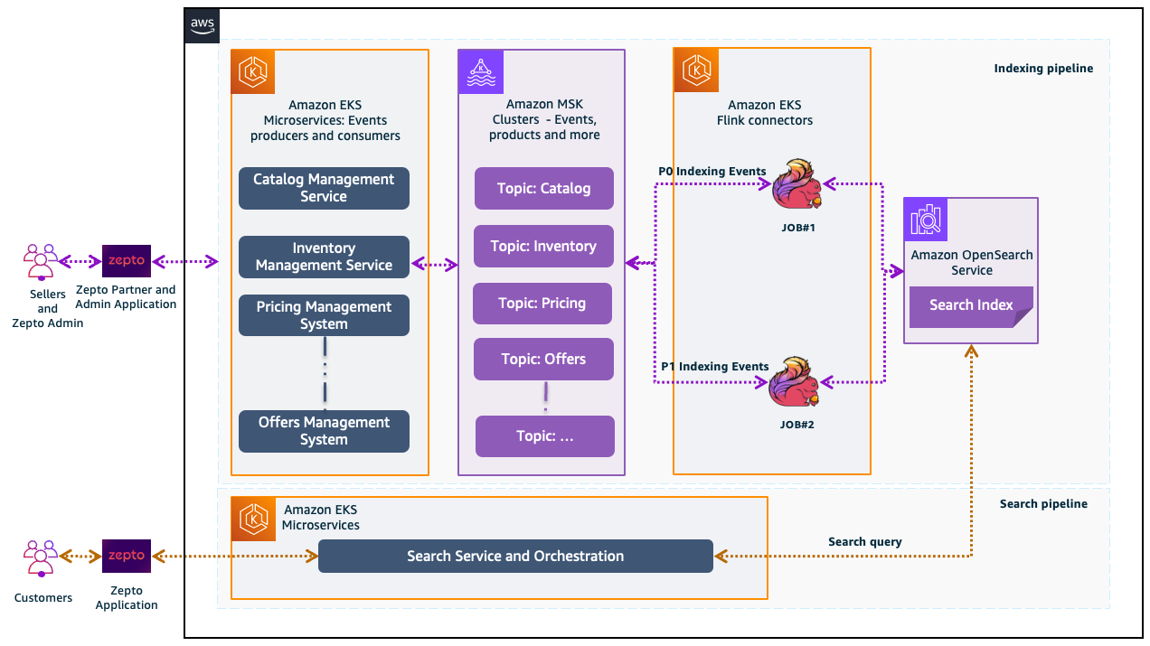
An event-driven architecture powers this experience, keeping results fresh as products, prices, offers, and inventory change across hundreds of delivery hubs. The following architecture diagram illustrates Zepto’s end-to-end indexing and search pipeline, from event production through stream processing to the search indices on OpenSearch Service.

Figure 1: Zepto’s end-to-end indexing and search pipeline architecture

Event producers and consumers: Zepto’s application microservices are deployed on Amazon Elastic Kubernetes Service (Amazon EKS), a fully managed service for running Kubernetes workloads on AWS. These microservices serve as both event producers and consumers. Sellers and Zepto Admin users interact with the Zepto Partner and Admin application.

Key microservices: The Catalog Management Service emits events when product metadata changes like new product additions, attribute updates, and category reclassifications. The Inventory Management Service publishes stock-level changes across delivery hubs in real time as warehouse teams pick, pack, and replenish inventory. The Pricing Management Service generates events whenever sellers update pricing. The Offers Management Service broadcasts events when promotional offers are created, activated, modified, or expired. Together, these microservices capture every relevant update for downstream indexing, producing events into the streaming layer whenever business state changes.

Search events streaming: All domain events flow through Amazon Managed Streaming for Apache Kafka (Amazon MSK), a managed streaming data service that manages Apache Kafka infrastructure and operations.

The system organizes events into dedicated Kafka topics by business domain. These include Catalog for product metadata changes, Inventory for hub-level stock updates, Pricing for price changes across stores, and Offers for promotional offer lifecycle events and more. This topic-based partitioning provides independent scaling per domain, ensures ordered delivery within each topic and consumer isolation, so that a surge in inventory events does not disrupt catalog indexing.

Stream processing and routing: Events from MSK topics are consumed and routed into two priority-based indexing pipelines through dedicated Apache Flink OpenSearch Connector jobs deployed on an Amazon EKS cluster:

  • Job #1: P0 indexing events (Pipeline #1): Processes high-priority events requiring near real-time index freshness, such as inventory changes, catalog enrichment, and pricing updates.
  • Job #2: P1 indexing events (Pipeline #2): Handles lower-priority but higher-volume events, such as tag updates, semantic embedding generation, offer activations, and nightly revenue per impression (RPI) score recomputation. These updates improve search quality but can tolerate slightly higher latency.

With this dual-job approach, Zepto maintains sub-second freshness for critical signals like stock availability and current pricing. Compute-heavy enrichment updates are processed separately without creating backpressure on real-time updates.

Search indices: Zepto hosts the search index on OpenSearch Service, structured at the city-product level. Delivery hub-specific metadata, such as stock status and hub-level demand signals, is stored as nested documents within each record. The following example depicts a typical document in the search index.

{
    "city": "mumbai",
    "product_id": "SKU-29401",
    "product_name": "Amul Butter 500g",
    "category": "Dairy",
    "offer_ids": ["OFFER-201", "OFFER-305"],
    "tags: [weekend, liquidation],
    "hubs": [
        {
            "hub_id": "MUM-HUB-01",
            "rpi_score": 0.0142,
            "stock_status": "in_stock",
            "hub_signals": {"demand": "peak"},
            "active": "true"
        },
        {
            "hub_id": "MUM-HUB-02",
            "rpi_score": 0.0147,
            "stock_status": "low_stock",
            "hub_signals": {"demand": "low"},
            "active": "false"
        },
        ..
    ]
}

The document structure supports store-level personalization while organizing the index by city-product pairs.

Search pipeline: Zepto’s search platform decouples the search request flow from the indexing pipeline at the application layer. When a customer initiates a search, the request passes through the Zepto application to the Search Service and Orchestration layer, which queries the OpenSearch index and assembles the response.

The Search Service and Orchestration layer handles the complete query lifecycle. This includes query understanding, candidate retrieval, machine learning (ML) ranking, ad slotting, and response assembly. For a detailed overview of Zepto’s full search architecture, refer to Building Search for a 10-Minute World on the Zepto engineering blog.

Scaling challenge

Zepto’s search platform started with a single use case, basic product search. As the business expanded, the platform introduced increasingly sophisticated experiences and each new experience added indexing signals to the pipeline like offer events, liquidation tags, pricing changes, ranking scores and more. All needed to be ingested and reflected in the index. Simultaneously, growing user traffic and the expansion of browse surfaces increased read throughput demands on the cluster.

The challenge was most acute during festive events like Diwali and New Year, when traffic surges required scaling to 1.4× the data node count. Although the cluster handled the node additions, the team needed to monitor shard relocation progress and validate that search latencies remained within service level agreements (SLAs) at each step. This operational overhead grew with each scaling event.

Adding more nodes to the cluster would address the immediate throughput constraints, but at the cost of proportionally higher infrastructure spend. To find a solution, Zepto set a clear goal: “Improve throughput without increasing the data node count.”

Solution overview

With the goal of keeping the node count intact, Zepto experimented with multiple configurations. One approach was resharding, adjusting the number of primary shards to better distribute the workload across existing nodes. However, load testing under production-representative traffic revealed that each resharding configuration degraded search latencies. The resharding operations themselves were also operationally expensive, requiring full index recreation, data migration, and extended validation windows.

The team needed a fundamentally different approach. The approach needed to improve throughput without adding nodes or resharding the index.

Evaluating OpenSearch Optimized instances

OpenSearch Optimized instances are an instance family purpose-built for workloads that require high indexing throughput with cost efficiency. They are commonly used for log analytics and time series use cases. These instances store data on Amazon Elastic Block Store (Amazon EBS) volumes for fast local access. Apache Lucene segments are synchronously replicated to Amazon S3, providing 11 nines of data durability.

Despite the common use case association with log analytics, we recommended evaluating OpenSearch Optimized instances type OR2 for Zepto’s product search workload. The team assessed two key criteria to determine viability:

Criterion 1: Does segment replication address the throughput bottleneck?

With document replication (the default on memory-optimized instances), every write is indexed on the primary shard and then re-indexed independently on each replica. This duplicates CPU work across the cluster. With segment replication on OpenSearch Optimized instances, segments are built once on the primary shard. They are then copied as complete files to replicas. This eliminates the duplicate indexing pipeline on replicas and frees their compute for serving search queries. Zepto’s workload involved continuous indexing from multiple pipelines that competed with search traffic. This separation was the key architectural advantage.

Criterion 2: Can the search platform tolerate the 10-second refresh interval?

OpenSearch Optimized instances use a 10-second segment replication refresh interval that is longer than the default one-second refresh on memory-optimized instances. This means newly indexed documents become searchable with up to 10 seconds of additional delay. The team evaluated whether this trade-off was acceptable for their search use cases.

Rahul Pradeep, Senior Architect at Zepto, explains:

“Out-of-stock or in-stock is not a primary parameter for retrieval. It is more like a tiebreaker. Relevance is our primary parameter. We retrieve hundreds of products in one query and then do a last-minute validation against our real-time inventory service. That is why we may not need one-second refresh.”

Zepto’s existing architecture where the Product Enrichment Service validates inventory after retrieval indicated that the 10-second refresh interval would not impact customer experience; see how Zepto built Product Enrichment at scale for further details. The migration was viable without any application-level changes.

Based on this evaluation, the solution involved migrating from memory-optimized Graviton-based data nodes to OpenSearch Optimized instances. This shift changed how indexing work is distributed across the cluster. Instead of a model where every node duplicates the full indexing pipeline, only the primary shard performs indexing, and replicas receive pre-built segments.

Load testing

To validate the hypothesis before committing to a migration, we designed a proof of concept, a load testing setup in their lower environment that mirrored production characteristics:

  • Baseline cluster with r7g.12xlarge instances and a parallel testing cluster with or2.12xlarge instances, having four nodes per cluster.
  • Identical shard configuration (X primary shards, Y replica, Z shard copies per node).
  • Simultaneous indexing and read load simulation.

Document structure improvements

In addition to validating the infrastructure change, the team identified an opportunity to optimize the document structure itself to further improve search latency. They added an active_hubs attribute to the base document, a flat array listing only the hubs where the product is currently stocked and active as shown in the following updated document structure.

{
    <City and product metadata>,
    "active_hubs: [MUM-HUB-01, MUM-HUB-03],
    "hubs": [
        {
            "hub_id": "MUM-HUB-01",
            "rpi_score": 0.0142,
            "stock_status": "in_stock",
            "hub_signals": {"demand": "peak"},
            "active": "true"
        },
        ..
    ]
}

The following table summarizes the key metrics from the load test comparing the r7g.12xlarge baseline cluster against the or2.12xlarge test cluster under identical conditions.

Metric r7g.12xlarge or2.12xlarge Change
Peak indexing lag ~12M docs ~6M docs 2X Faster
Indexing throughput Baseline 2× higher 100% Improvement
Search latency (p90) 187 ms 89.1 ms 52% Improvement
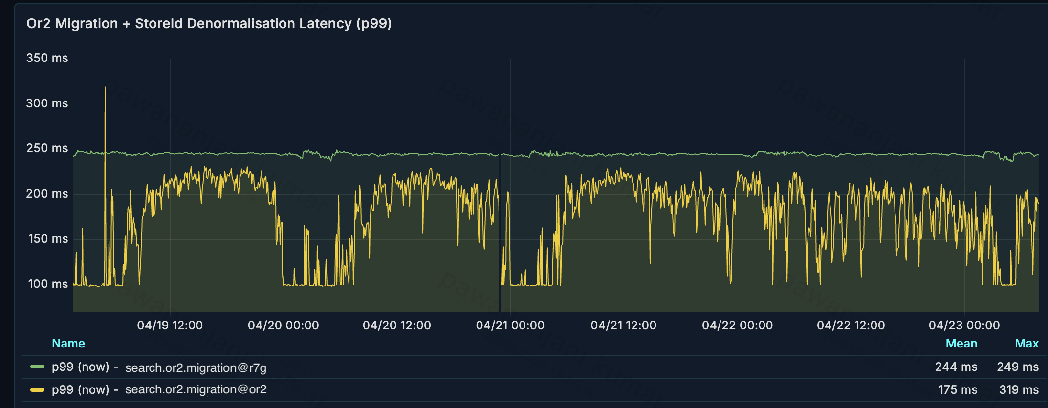
Search latency (p99) 244 ms 175 ms 28% Improvement

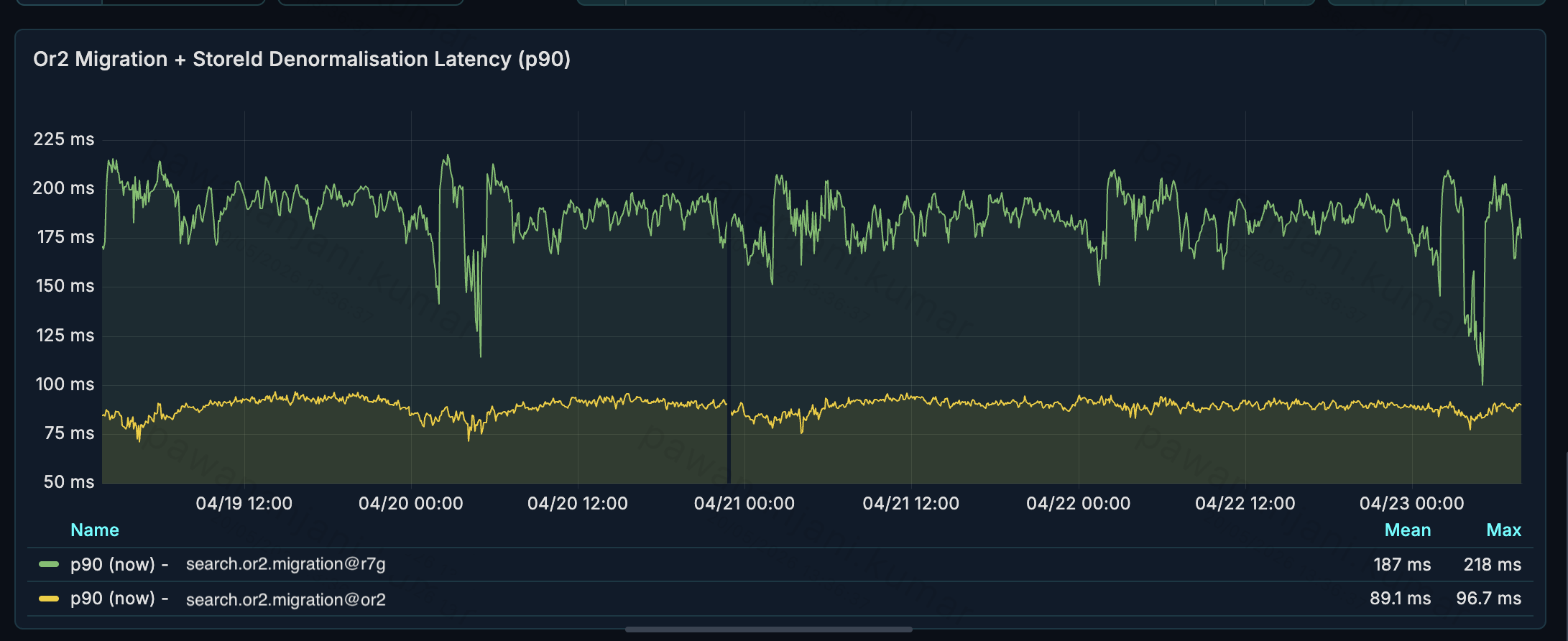
The following graph depicts the P90 search latency comparison between the two clusters.

Line graph comparing P90 search latency for the r7g.12xlarge and or2.12xlarge clusters over time

Figure 2: P90 search latency comparison between the r7g and OR2 clusters

The following graph depicts the P99 search latency comparison between the two clusters.

Line graph comparing P99 search latency for the r7g.12xlarge and or2.12xlarge clusters over time

Figure 3: P99 search latency comparison between the r7g and OR2 clusters

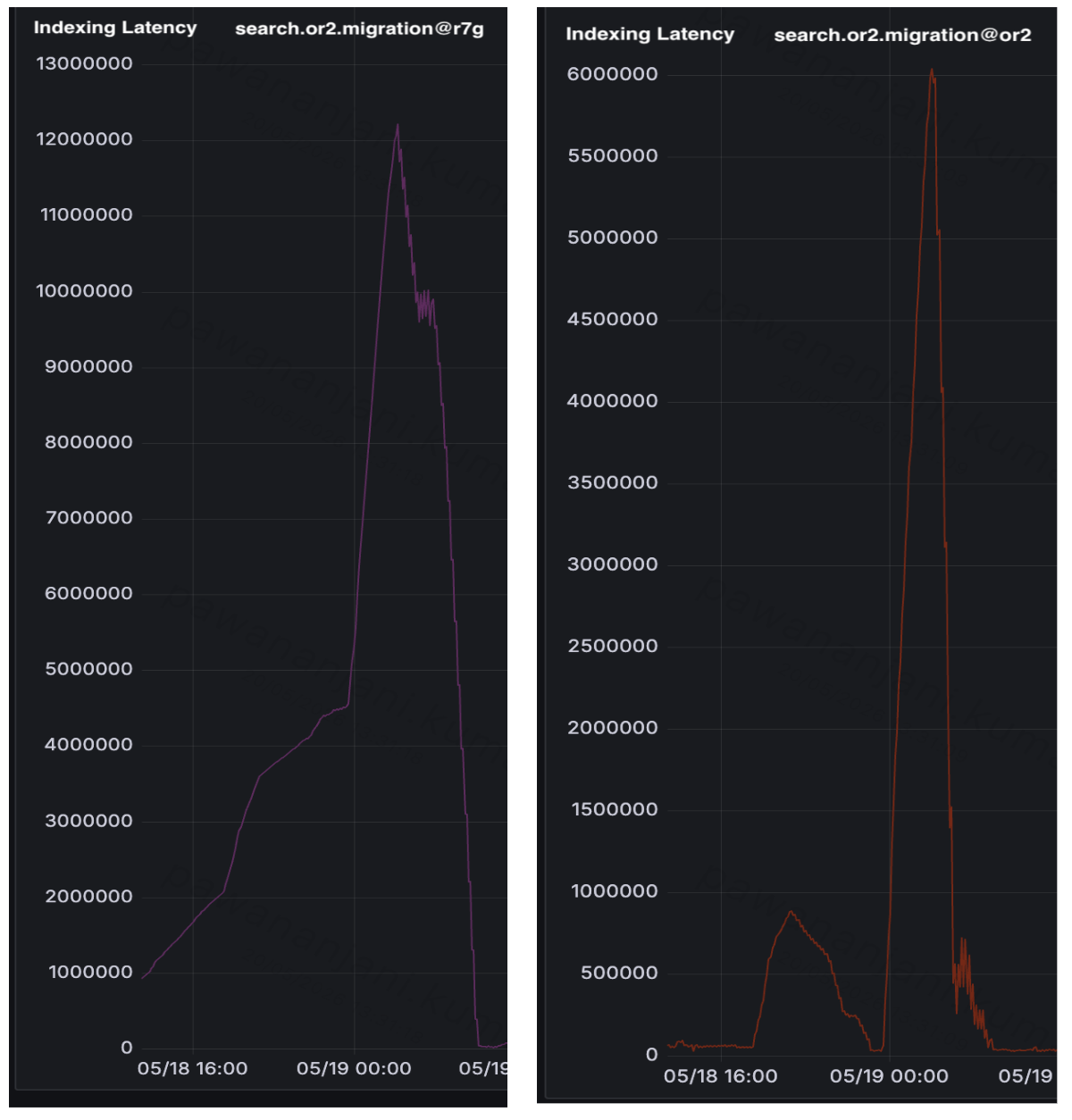
The following graphs depict the indexing latency comparison between the two clusters.

Figure 4: Indexing latency comparison between the r7g (left) and OR2 (right) clusters

Key insights

  • Improvement in indexing throughput: The higher indexing throughput of OR2 is most visible during nightly batch operations when events from RPI score recomputation, tag updates, and catalog enrichment flood the indexing pipeline simultaneously. On the r7g cluster, the P1 indexing lag peaked at over 12M docs. On OR2, with approximately 2× the indexing throughput, the same event volume produced a peak lag of only 6M docs. Higher throughput translates directly to lower lag and fresher search results. It is attributed to the segment replication approach of OR2 that eliminates redundant indexing work on replicas. Each document is indexed once on the primary shard rather than being replayed on each replica.
  • Reduction in search latency: P90 search latency dropped from 187 ms to 89.1 ms (52% improvement) and P99 from 244 ms to 175 ms (28% improvement). These gains are primarily attributable to the active_hubs document structure change rather than the instance type migration alone. By pre-computing a flat list of active hubs at index time, the query no longer needs to traverse nested hub documents to determine availability. This creates a lightweight pre-filter that eliminates unnecessary computation at search time.

Production planning and rollout

The load test results gave Zepto the confidence to make a key architectural decision: reduce the overall data node count. Higher per-node indexing throughput meant the same workload could be served with fewer nodes with OR2, and the cost savings compounded. Each eliminated node removed compute, storage, and operational overhead from the cluster. Zepto carried this forward into production, provisioning the OR2 cluster at two-thirds of the original node count. The following table summarizes the before-and-after comparison.

Metric r7g.12xlarge or2.12xlarge Change
Data nodes required 3X Nodes 2X Nodes -33.3%
Cost savings Baseline 2/3 of Baseline +30%

Rather than a complete cutover, Zepto adopted a phased rollout strategy using bucket-based traffic routing, completing the migration over approximately two months with zero downtime:

  1. Provisioned a new OpenSearch Service domain on OR2 instances with segment replication turned on.
  2. Executed parallel indexing pipelines to populate the OR2 cluster while the existing r7g cluster continued serving production traffic.
  3. Routed internal users to the OR2 cluster first to validate search quality, relevance, and latency characteristics under real query patterns.
  4. Gradually increased external user traffic in buckets, monitoring comparison dashboards at each increment for latency regressions or relevance drift.
  5. Maintained parallel dashboards throughout the migration to compare the OR2 and r7g clusters in real time. Key metrics monitored included p50 and p99 search latency, indexing throughput, replica lag, Java Virtual Machine (JVM) heap utilization, circuit breaker events, I/O operations per second (IOPS) utilization, and disk throughput.

Challenges and lessons learned

During the migration, the team encountered one notable challenge: latency spikes during segment merges. This observation offers practical guidance for teams evaluating OpenSearch Optimized instances for search workloads.

Symptom: After shifting significant traffic to OR2, Zepto observed intermittent p99 latency spikes correlating with segment merge operations.

Root cause: Large segment merges consumed significant I/O bandwidth, temporarily impacting concurrent search query performance. The original 256 GB EBS volumes did not provide sufficient IOPS buffer for concurrent merge and search operations.

Resolution: Implemented the following two changes:

  1. Increased EBS volume size to 1 TB per node. For gp3 volumes, baseline IOPS increase with volume size. This provided buffer for concurrent operations.
  2. Tuned the segment merge policy. Reduced max_merged_segment (see OpenSearch: Force Merge API for more details) from 5 GB to 2 GB and segments_per_tier (see OpenSearch: Index Settings for more details) from 10 to 5. This produces smaller, more frequent merges that distribute I/O load more evenly rather than infrequent large merges that spike latency.

After increasing EBS volume size and tuning the segment merge policy, latency spikes decreased. Transient spikes still occurred during merges but settled quickly within acceptable bounds.

Production cutover

Finally, Zepto shifted from partial to 100% traffic over four weeks and decommissioned the previous cluster after confirming stable performance across multiple peak traffic cycles. The following table summarizes the cluster configuration before and after migration.

Parameter Previous Cluster Current Cluster
Instance type r7g.12xlarge or2.12xlarge
Data nodes 3X Nodes 2X Nodes
RAM per node 384 GiB 384 GiB
Replication strategy Document replication Segment replication
Default refresh interval 1 Second 10 Seconds
Durability Cross-Availability Zone replicas S3 synchronous replication

Conclusion

In this post, we described Zepto’s evaluation of OpenSearch Optimized instances for latency-sensitive product search and the results of their production migration. By moving from memory-optimized data nodes to OpenSearch Optimized instances with segment replication enabled, Zepto achieved over 100% higher indexing throughput and 30% cost savings while reducing their cluster to two-thirds of the previous data node count.

Zepto’s migration demonstrates that OpenSearch Optimized instances are a viable choice for latency-sensitive product search and not just log analytics. Workloads where the retrieval layer can tolerate seconds-level staleness because real-time consistency is resolved at a different layer are candidates for adopting OR2 instances. For ecommerce and quick-commerce platforms that separate candidate generation from availability validation, this pattern can deliver significant infrastructure cost reduction.

If your workload has high indexing volume, and can tolerate a 10-second refresh interval, consider evaluating OpenSearch Optimized instances for your cluster. To get started:

  1. Assess your workload fit: review your current indexing throughput, replica count, and refresh interval requirements. Prioritize this approach if your workload has a high write-to-read ratio.
  2. Execute a proof of concept: provision a small OpenSearch Optimized cluster in a lower environment with identical shard configuration and restore a production index snapshot. Execute simultaneous indexing and search load to validate throughput and latency.
  3. Plan a phased rollout: use parallel indexing and bucket-based traffic routing to migrate incrementally with zero downtime, monitoring indexing lag and search latency at each step.

To explore the architecture behind OpenSearch Optimized instances, see Under the Hood: OpenSearch Optimized Instances. For practical configuration guidance, see Improve performance with OpenSearch Optimized Instances. We welcome your questions and feedback in the comments section below.


About the authors

Mayank Agarwal

Mayank Agarwal

Mayank is a Principal Architect at Zepto, focused on ML platforms, search, and supply-chain systems at scale. He writes about technology at agarwalknayam.com.

Kayalvizhi Kandasamy

Kayalvizhi Kandasamy

Kayalvizhi is a Principal Solutions Architect at AWS. She specializes in helping customers turn ideas into production-ready solutions using AI/ML, analytics, serverless, and microservices on AWS. A FIDE-rated chess player, Kayalvizhi enjoys passing on her love for the game by coaching her daughters.

Rahul Pradeep

Rahul Pradeep

Rahul is a Senior Architect at Zepto working across systems in the Shopping Journey of a user. His focus areas are to build high throughput systems in search, discovery and checkout domains that can stand the test of growing scale and changing business needs. He writes about tech at raahulpradeep.com

Bhagwati Malav

Bhagwati Malav

Bhagwati is an Engineering Leader at Zepto, building and scaling Search and Discovery systems. His work focuses on information retrieval, search relevance, semantic search, ranking systems, and distributed systems.

Pawananjani Kumar

Pawananjani Kumar

Pawananjani is a Senior Engineer on Zepto’s Search team. He works on the core mechanics of search retrieval, result ranking, and data indexing.

Rugved Sawarkar

Rugved Sawarkar

Rugved is a Senior Engineer within the Search team at Zepto. His primary responsibilities center on building and refining search retrieval, ranking algorithms, and indexing pipelines.

Harpreet Singh

Harpreet Singh

Harpreet is a Senior Technical Account Manager at AWS based in Bangalore, specializing in cloud optimization, resilience, and GenAI-driven operations. He develops innovative strategies to solve complex customer challenges across high-growth industries. He aims to drive cloud adoption and operational excellence at scale. Outside work, Harpreet enjoys playing badminton and exploring new technology.

Aashi Agarwal

Aashi Agarwal

Aashi is a Solutions Architect at AWS, where she specializes in the analytics domain. She guides customers through the transformative process of migration and modernization. With a blend of visionary architecture and robust security, she crafts resilient systems and seamlessly integrates cutting-edge AI/ML services, including the marvels of generative AI, into their technological tapestry. Outside of work, she loves to explore new things and discovers music.

AWS Weekly Roundup: EC2 application status checks, IAM role manager, OpenAI Daybreak on Bedrock, and more (August 17, 2026)

Post Syndicated from Channy Yun (윤석찬) original https://aws.amazon.com/blogs/aws/aws-weekly-roundup-ec2-application-status-checks-iam-role-manager-openai-daybreak-on-bedrock-and-more-august-17-2026/

Last week, the OpenSearch and Valkey teams visited Seoul to meet open source developers and contributors in the Open Source Summit Korea 2026 and MCP DevSummit Seoul 2026. At the four-day event, community leaders and users of open source projects and emerging agent AI gathered to share knowledge, collaborate on solutions, and push the projects forward.

Leaders of the Korean OpenSearch communities volunteered to participate in the booth, and also had time to network and interact in the user group meetup.

OpenSearch is an open source, enterprise-grade search and observability suite that brings order to unstructured data at scale. On June 9, 2026, OpenSearch 3.7 introduced new tools designed to query, alert, and track SLOs across logs, traces, and metrics through a single interface and retrieve vectors up to 5.5x faster for improved search performance. Since July 30, 2026, you can run OpenSearch version 3.7 on Amazon OpenSearch Service for improvements in vector search performance, search relevance, and Query Insights.

Valkey is an open source high-performance key/value datastore that supports a variety of workloads such as caching, message queues, and it can act as a primary database. On May 19, 2026, Valkey 9.1 introduced a redesigned I/O threading model that improves throughput by up to 17% and reduces memory usage for strings under 128 bytes by up to 20%. Since June 23, 2026, you can run Valkey 9.1 in Amazon ElastiCache for node-based clusters, delivering higher throughput, improved memory efficiency, and stronger access control for multi-tenant workloads.

You can meet our open source teams at upcoming OpenSearch and Valkey events.

Last week’s launches
Here are some launches that got my attention:

For a full list of AWS announcements, be sure to keep an eye on the What’s New with AWS page.

Other AWS news
Here are some additional projects and news items you may find interesting:

  • The deprecation of email validation in AWS Certificate Manager: ACM will discontinue support for email-validated public certificates by September 30, 2027. If you use email validation for your ACM public certificates, you need to migrate to DNS validation before that date. For Amazon CloudFront distributions, HTTP validation is also available.
  • The next-generation AWS VPN Client with CLI support and admin controls: You can use a new AWS VPN Client built on OpenVPN3. With the new client, you get full backward compatibility with existing AWS Client VPN endpoints while delivering the automation capabilities and security posture that enterprise networking teams have been asking for.
  • Oracle Exadata on Exascale for Oracle AI Database@AWS: ExaDB-XS brings Exadata-class performance and availability through a consumption-based model. With ExaDB-XS, you can scale compute and storage independently in small increments and pay only for what you consume.

For a full list of AWS blog posts, be sure to keep an eye on the AWS Blogs page.

Learn more about AWS, browse and join upcoming AWS-led in-person and virtual events, startup events, and developer-focused events including AWS Summits and AWS Community Days. Join the AWS Builder Center to connect with builders, share solutions, and access content that supports your development.

That is all for this week. Check back next Monday for another Weekly Roundup!

Channy

How Autodesk migrated 2.3 billion documents to Amazon OpenSearch Service using Migration Assistant and intelligent routing

Post Syndicated from Ambarish Rao original https://aws.amazon.com/blogs/big-data/how-autodesk-migrated-2-3-billion-documents-to-amazon-opensearch-service-using-migration-assistant-and-intelligent-routing/

OpenSearch is an open source software suite for search, analytics, security monitoring, and observability applications, licensed under the Apache License V2.0. Amazon OpenSearch Service is a managed service that lets you deploy, scale, and operate OpenSearch and the Elasticsearch engine in the AWS Cloud. Customers run search workloads on OpenSearch Service at a scale of billions of documents. When a single index holds millions to billions of documents, you need to plan the topology of the OpenSearch Service domain that holds the index. This post walks through how Autodesk re-architected a single-index Elasticsearch 7.1.1 domain on Amazon OpenSearch Service into four multi-index OpenSearch Service domains, using Migration Assistant for Amazon OpenSearch Service and a routing layer that directs each query to the shards that hold the data for that query.

Autodesk is a technology company that serves customers across three industry verticals: Architecture, Engineering, and Construction (AEC), Product Design and Manufacturing, and Media and Entertainment. Autodesk’s mission is to empower everyone, everywhere to design and make anything, helping customers work across the boundaries of project, discipline, and industry.

Autodesk Forma (formerly Autodesk Construction Cloud, or ACC) is a cloud-based construction management and collaboration system. Customers across the globe use Autodesk Forma for workflows that include document management, bid management, quantification, coordination, design collaboration, project management and field collaboration. Autodesk Forma uses Amazon OpenSearch Service to provide a search experience for millions of users. As customers add data, the data that Forma stores in OpenSearch Service grows. In an OpenSearch Service domain, an index is the unit of data storage and organization. When an index reaches 100 TB, the index becomes a performance bottleneck and is hard to scale. As Autodesk Forma grew, Forma data management (formerly Autodesk Docs) hit performance and scaling limits. This component supports access and search across the project catalog.

Where Autodesk started

Forma data management ran on a single Elasticsearch 7.1.1 domain on Amazon OpenSearch Service with one index. The domain held about 100 TB of data on over 100 data nodes with over 400 primary shards and a replication factor of 1. The average shard held 200 GB. Because of the scale and the production state of the domain, tuning techniques such as adding shards, adding indices, or rebalancing data were not viable.

The single-index, single-domain design exposed three challenges to future data growth:

  1. Query performance. Query latency degraded over time as data grew.
  2. Vertical scaling. The team had reached the limit of the largest Amazon Elastic Compute Cloud (Amazon EC2) instance size available for the existing instance class.
  3. Horizontal scaling. Without a routing mechanism, adding nodes produced hot nodes inside the cluster managed by the OpenSearch Service domain.

Multi-domain architecture with intelligent routing

Vertical or horizontal scaling can address query performance in the short term, but neither addresses the underlying single-index, single-domain scalability limit. A horizontal scaling approach that uses routing keys gives you control over which shards each query touches, without requiring larger hardware. The Autodesk team applied this approach to re-architect the search service without impacting production traffic.

Four Amazon OpenSearch Service domains with an Amazon DynamoDB routing layer directing each query to the correct domain

Figure 1: Multi-domain architecture with intelligent routing

The architecture has the following properties:

  • Four Amazon OpenSearch Service domains on OpenSearch 2.19, each running 24 m7i.4xlarge.search nodes.
  • 24 indices total (6 per domain).
  • About 95 million documents per index.
  • 52 TB of primary storage. This is 37 percent smaller than the primary storage size of the original single-index domain, mainly because the migration skipped deleted documents.

The setup uses four horizontally scaled OpenSearch Service domains, with a routing layer that directs each query to the domain that holds the project’s data.

The architecture uses a Amazon DynamoDB table that stores 4.3 million routing records, one record per project. A project is the primary workspace in Forma data management, where teams, data, documents, models, workflows, permissions, issues, and collaboration activities live together. Forma application looks up the Amazon DynamoDB table for the project-to-domain mapping and then issues the search query to the correct domain.

Redistributing millions of records across four domains was hard. To find an even project-to-index allocation, the team used a bin-packing algorithm. A bin-packing algorithm packs items of varying sizes into a fixed number of bins to minimize waste and produce an even distribution. The team worked with 4.3 million projects of varying document counts, from a few documents per project up to millions, across 24 indices that each target around 400 million documents. The team implemented a stratified bin-packing algorithm that uses historical usage metrics for the workload. This algorithm avoids over- or under-allocation of resources during migration planning. To avoid over-allocation, the team used the 95th percentile (P95) usage metric. After applying the algorithm, each OpenSearch Service domain landed at about 49 percent utilization, which leaves a 2x growth buffer. The application then uses routing-key-based queries to search only the relevant shards, instead of every shard in the index.

The architecture has the following benefits:

  • Horizontal scalability. The team can add more domains and indices as needed.
  • Efficient routing. Queries hit specific shards, not every shard in the domain.
  • Reduced blast radius. If one domain becomes unavailable, only about 25% of traffic is affected, instead of full downtime under the single-domain design.
  • Independent scaling. The team can scale each domain based on its load pattern.
  • More search threads. The aggregate search-thread pool is larger across four domains than on one domain.

Migration steps

The following sections describe the four steps the Autodesk team followed to complete the migration.

Step 1: Categorize projects by size

The team grouped projects into four size categories by current document count, then collected data over six months to compute a per-category growth factor and extrapolate one year out:

Category Document range Project count % of total P95 growth factor Rationale
TINY 0 – 1,000 4,085,310 95.0% 3.82x Tiny projects grow fastest
SMALL 1,000 – 10,000 184,347 4.3% 2.11x Moderate growth expected
MEDIUM 10,000 – 100,000 28,385 0.66% 1.72x Slower relative growth
LARGE 100,000+ 2,266 0.05% 1.38x Already mature, minimal growth
Total 4,300,308 100%

The table shows that 95 percent of projects are TINY, but LARGE projects account for the bulk of document volume. The stratification by category lets the algorithm handle each category appropriately.

The Autodesk team analyzed document count per project over six months to estimate growth. Using the P95 growth factor per category gives a conservative capacity plan that covers 95 percent of projects and avoids over-provisioning.

Step 2: Interleaved distribution

If you process all LARGE projects first, you create imbalance across the indices. To avoid this imbalance, the bin-packing algorithm interleaves the categories in a round-robin pattern. The team used the following sequence to distribute documents evenly across the Amazon OpenSearch Service domains:

  1. Sort the projects within each category, largest first.
  2. Create a queue for each category. The queue is a first-in, first-out data structure that holds the sorted projects for one category.
  3. Distribute projects in a round-robin pattern: pick one from LARGE, then MEDIUM, then SMALL, then TINY, and repeat.

Step 3: Load-balanced best fit

After interleaving, the team computed the projected size of each project and assigned the project to an index. The following steps describe the approach:

  1. Compute the estimated future size as current size × growth factor.
  2. Use a priority queue to find the index with the most available capacity. In a priority queue, each element has a priority. Here, the priority of each index is the amount of available capacity the index has. Unlike a regular queue, a priority queue returns the highest-priority element first, not the first one inserted.
  3. Assign the project to the index that has the most available capacity.
  4. Update the index’s estimated load and re-insert the index into the priority queue with the new capacity. The re-insert step keeps the queue accurate for the next project assignment.

The preceding three steps produced the following results:

  • The algorithm distributed 4.3 million projects with 99.999 percent routing accuracy.
  • Project distribution across indices held to a 0.15 percent variance.
  • Each domain landed at 49.1 percent capacity utilization after applying growth factors, leaving 50.9 percent headroom for future growth.
  • The algorithm computed the 4.3 million project allocations in about 10 minutes.

The team stored the project-to-index allocation mapping in Amazon DynamoDB for real-time query routing. Routing controls how the application uses domain resources and how each domain performs. With routing, the application searches the shards that match the routing key (projectId) for that project. Without routing, the same query searches every shard in the index, which wastes domain resources and produces slower queries. The team also tuned the shard size, which matters most for large projects. One of the largest projects held 7 million documents at about 40 KB per document, for a total of about 280 GB. To split the data for that project into 20–25 GB shards, the team set routing_partition_size to 12.

Step 4: Migration with Migration Assistant for Amazon OpenSearch Service

The Autodesk team used the snapshot and re-index path in Migration Assistant for Amazon OpenSearch Service to migrate 2.3 billion documents. Migration Assistant for Amazon OpenSearch Service adapts to the migration profile and provides AWS Identity and Access Management (IAM) permission boundaries, Amazon Virtual Private Cloud (Amazon VPC) support, and the security policies the migration needs. Migration Assistant for Amazon OpenSearch Service integrated with the over 400 tasks that run the application on Amazon Elastic Container Service (Amazon ECS) with AWS Fargate.

Before the production cutover, the team ran several proof-of-concept (PoC) iterations and tuned the migration configuration to raise throughput from 18 GB/hr to 228 GB/hr. The first PoC iteration hit 18 GB/hr on m7g.large.search nodes. Each subsequent iteration added horizontal scale, larger instances (m7g.2xlarge.search and m7g.4xlarge.search), parallel writes across domains, and zero replicas during migration. The fourth and final PoC iteration hit 228 GB/hr. Multiple PoC iterations helped the team select the optimal instance size and instance class to migrate 2.3 billion documents in 6 hours with zero downtime and no customer incidents.

Post-migration analysis

After the team migrated 2.3 billion documents with routing enabled, the shards landed as follows:

Metric Result Target Status
Total primary shards 4,325
Total data size 52.11 TB ~52 TB ✓ On target
Average shard size 12.34 GB 10–15 GB ✓ Optimal
Median shard size 11.9 GB 10–15 GB ✓ Optimal
Shards in optimal range (10–15 GB) 75.5% 70% ✓ Above target
Hot shards (> 30 GB) 12 (0.28%) < 1% ✓ Within limit
Undersized shards (< 10 GB) 528 (12.2%) < 15% ✓ Within limit
Cross-domain balance 2.3% variance < 5% ✓ Within target
Node balance (StdDev) 0.78–1.12 shards < 2 ✓ Within target

The following table compares the pre- and post-migration architectures:

Aspect Old (single domain) New (four domains with intelligent routing)
Shard size 200 GB average 12.34 GB average (94% reduction)
Query broadcast All 400+ shards ~12 shards (97% reduction)
Shards in optimal range 0% 75.5%
Cross-domain balance N/A (single domain) 2.3% variance
Storage 83.3 TB 52 TB
Total P99 query latency 17 seconds 5 seconds

The team migrated 2.3 billion documents in about 6 hours. Storage dropped by about 37 percent, from 83.3 TB to 52 TB, because the migration dropped deleted documents. The migration produced 4,325 shards at an average of 12.34 GB per shard, distributed across the four domains. 75.5 percent of shards landed in the 10–15 GB range, compared to 210 GB before the migration, which confirms that the new architecture solves the large-shard problem. The shard size is as per general guidance where search latency is a key performance objective. Cross-domain variance of 2.3 percent (12.85 TB to 13.15 TB per domain) confirms even data distribution.

After the migration, queries that include the projectId routing key scan only the relevant shards (typically 12 of 180 per index), which reduces search load across shards by 93 percent. Routing also balances CPU and memory use across each domain. The routing_partition_size of 12 per index produced the right shard count per index. Overall P99 latency improved by 72 percent, from 17 seconds to 5 seconds. Within that figure, search-query P99 improved by 92 percent, from 2,500 ms to 200 ms.

Lessons learned

The PoC iterations surfaced several lessons. Larger instance types help query performance in the short term, but query routing combined with horizontal scaling produces higher sustained throughput. During bulk loads, disable replicas and increase the refresh interval to reduce write overhead. Plan for enough IP addresses and subnet capacity when you scale the application out, so that you do not hit a service limit mid-migration. Validate the VPC routing configuration between the application and the OpenSearch Service domains. Confirm OpenSearch Service data-node capacity with AWS Support before a horizontal scale-out. The Amazon DynamoDB-based routing layer adds about 20 ms of routing latency per query, but the routing layer cuts overall search latency and unlocks horizontal scale.

Conclusion

In this post, you saw how the Autodesk team migrated 2.3 billion documents from a single-index domain to four multi-index Amazon OpenSearch Service domains in about 6 hours.

Transitioning to a multi-domain architecture or updating to the latest OpenSearch version has historically been complex. It can also be difficult to predict the outcome of a migration before production traffic moves. The Migration Assistant for Amazon OpenSearch Service solution addresses these challenges by making migration workflow-driven, repeatable, and more straightforward to validate before cutover.

Migration Assistant for Amazon OpenSearch Service coupled with Amazon DynamoDB-based intelligent routing helped achieve balanced shards and improved search query performance. Multiple PoC iterations helped find routing bugs, service-quota limitations, and infrastructure-provisioning gaps before the production cutover.

If you plan to migrate a large dataset between OpenSearch Service domains, you can use Migration Assistant for Amazon OpenSearch Service. For more information, see the Migration Assistant for Amazon OpenSearch Service documentation.


About the authors

Ambarish Rao

Ambarish Rao

Ambarish is a Principal Engineer at Autodesk Search Team. He is based out of Pune. With 11 years of experience across financial data, logistics and now design and manufacturing, he has worked on mid to large scale distributed systems. When not working on Search, he’s either swimming, playing badminton, volunteering to teach kids, or hunting for Pune’s best biryani.

Chengsi Xie

Chengsi Xie

Chengsi is a Software Development Engineer on Autodesk Search Team. He is focused on building scalable distributed search platforms. He enjoys digging into the root causes behind problems and understanding how systems behave. Outside of work, he likes to stay active through running, playing badminton, hiking, and other outdoor activities that help him stay energized and grounded.

Manoj Kale

Manoj Kale

Manoj is a Senior Solutions Architect at Amazon Web Services. He helps customers design and build scalable, resilient solutions on AWS. He specializes in cloud architecture, AI/ML, and DevOps, and enjoys working with customers to solve complex technical challenges. Outside of work, he likes to spend time with family, travel and log the travel through travel logs and photos.

Anirudh Gupta

Anirudh Gupta

Anirudh is a Technical Account Manager at Amazon Web Services. He works closely with enterprise customers to help them architect, optimize, and operate their workloads on AWS. He is passionate about helping customers modernize their infrastructure and scale distributed systems on AWS.

Priyanshi Omer

Priyanshi Omer

Priyanshi is a Solutions Architect at Amazon Web Services. She helps customers design and build scalable, resilient solutions on AWS. She specializes in cloud architecture, AI/ML, and DevOps, and enjoys working with customers to solve complex technical challenges.

Trace cascading decision failures with a blame graph on Amazon OpenSearch Service

Post Syndicated from Jon Handler original https://aws.amazon.com/blogs/big-data/trace-cascading-decision-failures-with-a-blame-graph-on-amazon-opensearch-service/

Multi-agent systems are straightforward to build but hard to debug. You chain a few agents together, each one does its part, and most of the time it works. When it doesn’t, you’re left with a large volume of logs. They tell you what every agent said, but nothing about which agent caused the bad outcome.

Working with AWS customers building multi-agent systems, we kept seeing the same problem. A pipeline of agents decides, the decision turns out wrong, and no one can say which agent caused it. The logs are complete, but they don’t answer that question. So we, two AWS Solutions Architects, built a stock-research pipeline to reproduce it and show a solution approach.

Five agents work in sequence, and the last one makes a BUY, SELL, or HOLD call. In our test cases, the agent kept recommending BUY, and the positions kept losing money. Every step was logged. The logs still didn’t tell us who broke the pipeline.

In this post, we show you how to build a blame graph that traces which agent caused a failure in a multi-agent pipeline, using Amazon OpenSearch Service for graph storage and Amazon Bedrock for embeddings and reasoning.

Prerequisites

You must have the following prerequisites to follow along with this post.

  • Download the source code from the GitHub repository: It includes everything needed to set up and run the demo end to end:
    • The five-agent pipeline.
    • The instrumentation layer.
    • AWS CloudFormation template.
    • OpenSearch UI dashboard export
    • Sample data.
    • Step-by-step setup instructions (README.md, DEPLOYMENT.md).
  • An AWS account with access to Amazon Bedrock (Anthropic Claude Sonnet 4.5 and Amazon Titan Text Embeddings V2 enabled in us-west-2).
  • An OpenSearch Service domain.
  • Python 3.11+.
  • AWS Command Line Interface (AWS CLI) v2 configured with valid credentials.

The challenge

The pipeline is a chain of five agents. A Researcher gathers the facts, a Risk Analyst weighs the downside, a Valuation Analyst runs the numbers, and a Macro Economist sets up the market backdrop. Each one builds on the output of the agents before it. The Strategist (AI agent) sits at the end and turns all of it into a single call: BUY, SELL, or HOLD.

We set up three failures, each one a pattern common in production agent deployments (hallucinated facts from retrieval, suppressed minority signals, stale data from delayed ingestion):

  • A hallucination. The Researcher invents a company partnership that doesn’t exist.
  • A buried warning. The Risk Analyst flags a regulatory risk and gets outvoted.
  • Stale data. The Researcher misses a filing published three days earlier.

We engineered each failure deterministically, so the demo is reproducible and has a known answer. For each scenario, we hand-authored the five agents’ outputs as fixed JavaScript Object Notation (JSON). The pipeline replays these outputs while the instrumentation computes embeddings, influence, and blame live. We recorded a ground-truth root cause (for example, researcher for hallucination).

In every case, the pipeline recommends BUY, and the position drops. Standard logging records each agent’s output, but it can’t tell you which claim drove the final decision. Closing the gap between logging and root-cause attribution is what we set out to do.

Solution

We treat agent reasoning as a graph and measure influence between agents, then walk that graph backward from the failed decision to find the root cause.

Three services make up the stack:

  • Strands Agents runs the five-agent pipeline.
  • Amazon Bedrock provides the models: Amazon Titan Text Embeddings V2 to embed each claim, and Anthropic Claude Sonnet 4.5 for agent reasoning and the incident write-up.
  • AOpenSearch UI applicationan analytics interface hosted in the AWS Cloud with a single endpoint, connects to the domain as a data source and serves the dashboard, Discover, and the Dev Tools console we use to investigate. 

Here is how blame attribution works. Every claim an agent makes becomes a document with an Amazon Titan embedding. When a downstream agent cites something, we measure the cosine similarity between that citation and each upstream claim. Cosine similarity becomes the influence one agent had on another.

We store these as edges. To find the root cause, we start at the failed decision and walk backward through the edges. Whoever contributed the most gets the most blame.

Alongside the graph we record three things per run: an explainability score for how much of the decision traces back to evidence, the confidence of the attribution, and whether a dissenting agent was overruled.

A note on method: there is no industry standard yet for root-cause attribution in multi-agent large language model (LLM) pipelines. Our approach combines two established ideas: a credit assignment (attributing an outcome to the steps that produced it) and embedding similarity for tracing how claims propagate, with an LLM-as-a-judge style check. The metrics here (influence, explainability) are pragmatic, reproducible measures we define in this post, not standardized benchmarks.

Architecture

Five parts make up the flow:

  • Agents run on the Strands Agents, with reasoning on Claude Sonnet 4.5.
  • An instrumentation layer extracts each claim, embeds it with Amazon Titan Text Embeddings V2, scores influence with cosine similarity, runs the backward traversal, and generates an incident report.
  • Amazon OpenSearch Service holds seven indices, including the claims index with k-nearest neighbor (kNN) vectors and the blame, metrics, and incident indices.
  • Analysts review the results in the OpenSearch UI application (the dashboard, Discover, and the Dev Tools console), launched from the Amazon OpenSearch Service console.
  • We use OpenSearch UI rather than the domain’s built-in dashboards. Because OpenSearch UI is hosted in the AWS Cloud, the application stays available during domain maintenance and can bring multiple data sources into one view. The pipeline still writes to the domain, and OpenSearch UI reads it as a registered data source. 
Five-agent pipeline: Researcher, Risk Analyst, Valuation, Macro Economist, Strategist in sequence, ending at BUY decision.

Figure 1a: The five-agent runtime pipeline

Instrumentation layer sending embeddings and blame edges to Amazon OpenSearch Service, with Amazon Bedrock providing Amazon Titan and Claude models.

Figure 1b: The instrumentation and OpenSearch Service data plane

Walking through a failure

We ran the pipeline nine times, three runs per scenario, on an Amazon OpenSearch Service domain running OpenSearch 2.17. The decision under investigation is the final BUY. We know it failed because each scenario carries a ground-truth outcome: the position lost money. The failure is the known bad outcome we trace backward from, not something the system infers.  Everything the pipeline produces is a document you can query, so the investigation is a series of queries we run from the Dev Tools console in the OpenSearch UI application. 

To follow along, launch the OpenSearch UI application from the Amazon OpenSearch Service console, open your workspace, and choose Dev Tools (near the bottom of the left navigation panel). Paste each query below into the left pane and choose the run button. Every query in this section is in the repository at devtools_queries.md, in the same order as the walkthrough, so you can copy them from there instead of retyping. The equivalent queries as Python are in queries.py. 

Start with the outcome

Every run is a BUY, and every loss is negative, down to 72 percent. Standard logging stops here. You know it failed, but you don’t know who to fix.

Dev Tools query results showing nine pipeline runs, all recommending BUY with losses from 58% to 72%.

Figure 2: Pipeline run results: all nine runs recommend BUY with losses up to 72%

Next, look at who influenced whom

Among all agents, the Researcher sources the most edges. Nearly every node downstream gets its data from the Researcher, making it the first place to look. A lead, not a verdict.

Dev Tools aggregation showing influence edges by source agent; Researcher has the most edges.

Figure 3: Influence edges aggregated by source agent

Query the blame metrics for each scenario

Blame lands on the Researcher, with a score around 0.45, and the attribution is correct on all three runs. A fabricated partnership flowed straight into the final BUY. Stale-data scenario behaves the same way: the Researcher again, at 0.46, correct.

Dev Tools query showing root cause attribution: Researcher at 0.45 for hallucination scenario.

Figure 4: Root cause attribution for hallucination runs

Here are the raw edges in Discover, sorted from highest influence to lowest

In the OpenSearch UI application, choose Discover and select the agent-blame index pattern, then set the time range to Last 30 days and sort by influence_score descending. Each row is one edge- a claim passed from a source agent (source_agent.agent_id) to a downstream agent (target_agent.agent_id), scored by how strongly it shaped that agent’s output. The top rows are the highest-influence edges: the ones that most shaped the final BUY.

Discover view of blame edges sorted by influence score, highest to lowest.

Figure 5: Blame edges sorted by influence score

When attribution is hard

It’s the buried-warning scenario that the graph gets wrong, and it’s the most useful result in the post.

The Risk Analyst was right. It flagged the regulatory risk. The Strategist saw the warning, weighted it at 0.15, and bought it anyway. Who actually failed? The Strategist.

But the blame graph points at the Risk Analyst, with the highest score in that run at 0.37. Why? Our method measures influence, and the dissent is a distinct claim that the method traces directly, so it scores high. Influence is not the same as responsibility.

Why did the Strategist ignore it? In the scenario, the Strategist acknowledged the dissent but reasoned that the strength of the clinical data made the compound “differentiated” from past failures. It weighted that bullish evidence at 0.85 against the Risk Analyst’s 0.15. The Strategist rationalized the warning away instead of treating high-confidence, time-bound regulatory risk as a hard stop. The model recorded that reasoning, which is exactly why we can see how the dissent was discounted.

This gap between influence and responsibility is why we track dissent on our own.

Dissent was present, acknowledged, and weighted at 0.15. A flag catches what the graph misses: a valid warning was heard and then ignored. One signal is not enough. Influence tells you what is propagated. Dissent flags tell you what was wrongly dismissed. You need both.

Dev Tools query showing suppressed dissent: dissent_weight_given 0.15, dissent_suppressed true.

Figure 6: Suppressed dissent detection

Reviewing the metrics dashboard

OpenSearch UI rolls up all nine runs. To open it, launch the OpenSearch UI application, open your workspace, and choose Dashboards in the left navigation, then open the Multi-Agent Blame Game — Observability dashboard. Set the time range to Last 30 days to see all nine runs. If you haven’t imported it yet, go to Manage Workspace and choose Import under Assets. Upload blame-game-dashboard.ndjson from the repository, mapping the index patterns to your domain’s data source.

Full OpenSearch metrics dashboard with panels for root cause, explainability, loss, influence, and propagation.

Figure 7: Full metrics dashboard

Each panel earns its place. A few are worth calling out. Root cause distribution flags the Researcher six times and the Risk Analyst three times. That Risk Analyst slice is the dissent misattribution from earlier, not a real culprit.

Root cause distribution: Researcher in 6 runs, Risk Analyst in 3 (misattribution).

Figure 8: Root cause distribution

Explainability averages 0.826, a metric we define, not a standard score.

Explainability score averaging 0.826 across nine runs.

Figure 9: Explainability score

Preventable loss versus realized loss splits the damage attribution can pin on one agent from the damage it can’t. And average influence clusters rather than spikes, showing no single cause. That is the whole reason attribution sums influence instead of trusting one edge.

Preventable loss panel showing dollar amounts attributed to root-cause agent per scenario.

Figure 10: Preventable loss

Realized loss panel showing total financial damage across all runs before attribution.

Figure 11: Realized loss

Blame and loss comparison table: hallucination and stale-data rows show small errors. Dissent row shows largest gap.

Figure 12: Blame and loss table

Average influence by source agent: scores cluster between 0.29 and 0.42, no single spike.

Figure 13: Average influence by source agent

Propagation type breakdown: most edges weak or independent, few amplified.

Figure 14: Propagation type breakdown

Exploring it interactively

For demos we wrapped the same pipeline in a small Streamlit app. To run it, from the repository root install the dependencies and start the app:   

source .env 
streamlit run src/app.py --server.address localhost

It opens in your browser at http://localhost:8501. It runs two ways: pick a prepared scenario and replay it, or type in a company of your own and have the five agents run live on Amazon Bedrock against it. Either way you watch the agents execute, and the blame graph form, with the verdict and the incident narrative on one screen. A History tab reads the metrics index, so you can review past runs without leaving the app. 

A live run has no ground truth, so the app doesn’t claim the attribution is right or wrong. You just see where the influence landed. The prepared scenarios are still the way to demonstrate a specific, known failure. 

Streamlit demo app showing a pipeline run with agent panels, claims, and blame verdict.

Figure 15: Streamlit demo app

Explaining every decision: The evidence each agent weighed

Blame attribution is only useful if you can see the evidence behind it. Every claim an agent makes is stored with the confidence the agent assigned and the source it came from. Sources include an SEC filing, a clinical trial registry, an FDA page, or an earnings call. A blame score is never a bare number. You can open any agent and read the exact claims and sources it weighed before it spoke.

Consider the final decision as the clearest example. The Strategist doesn’t only emit a BUY. The Strategist records which upstream claim it relied on and how much weight it gave each one. Recording those weights turns the last step from a black box into a list of citations you can audit.

Explainability captures exactly that. A high score means most of the recommendation traces back to specific, sourced claims rather than to unexplained reasoning. It is the difference between the model said BUY and the model said BUY because of these claims, from these sources, weighted this way.

Streamlit app detail: Financial Researcher claims expanded with confidence scores and sources.

Figure 16: Per-agent evidence and reasoning for the BioGenX run

Performance and results

Across nine runs, the system identified the correct root cause six times, or 67 percent. The three misses are all the buried-warning scenarios, where influence and responsibility diverge. We would rather report the real number and explain the miss than round it up.

A full run takes about 25 seconds from end to end. Almost all of that is the Bedrock calls: about 74 embeddings per run plus one Claude write-up.

Attribution alone, the part that walks the graph and assigns blame, runs in about 74 milliseconds. That is cheap enough to run on every pipeline execution, not only after something goes wrong.

End-to-end latency chart: full run about 25 seconds, attribution step about 74 milliseconds.

Figure 17: End-to-end latency scenario

What this means for building agent pipelines

Our data points at three concrete changes:

  • Make the Researcher cross-check any major claim against a second source.
  • Give the Strategist a hard rule so a high-confidence dissent near a binary event can’t be overridden silently.
  • Add a freshness check so old data can’t drive a decision.

More broadly, treat influence and responsibility as separate questions. Measure both. A blame graph is a strong default for tracing propagation, but you need side signals like dissent suppression to catch up on the cases it can’t see.

From detection to prevention: Guardrails that stop the loss

Attribution tells you who broke a run after the fact. The same signals can stop the break before anyone acts on it. We added a guardrail layer that sits between the pipeline’s decision and the action, and overrides the call when a known failure pattern appears. The demo implements this layer (run with --guardrails, or toggle it in the app). It answers the question of whether the fixes are in the code: they are.

Guardrail gate diagram: blame signals feed three checks (dissent-override, source cross-check, freshness) before decision passes or is held.

Figure 18: The guardrail gate between the decision and the action

Each guardrail targets one of the three failure modes:

  • Dissent-override (Strategist): When the Risk Analyst raises a high-confidence dissent near a binary event and the Strategist under-weights it, the decision is forced to the safe action (HOLD).
  • Source cross-check (Researcher): A material claim resting on a single self-reported source cannot drive a BUY. It must be corroborated, or the call is held.
  • Freshness (Researcher): If material information was published just before the analysis and was not reflected in the inputs, the call is held.

With all three enabled, every scenario that previously issued a losing BUY is caught and held. Across the three runs that is about USD $3.79 million of illustrative loss prevented.

Guardrails effect: approximately $3.79M illustrative loss converted from realized to prevented.

Figure 19: Guardrails convert realized loss into prevented loss

The three guardrails are demo-grade heuristics, and we want to be explicit about that. The single-source and freshness checks work here only because the scenario data is engineered with known sources and dates. They are proxies, not real controls. A well-formed hallucination with a plausible citation would pass without detection of the cross-check, and the freshness rule only knows about data it is handed.

To make this production-grade, replace each proxy with real control.

For hallucinations, don’t count sources. Verify the material claims a decision rests on against a trusted source such as a knowledge base in Amazon OpenSearch Service or an authoritative filings and market-data API. Use an entailment or LLM-as-a-judge check to confirm the evidence actually supports the claim, requiring corroboration from independent sources before a claim can drive a BUY.

For freshness, wire in a live data feed and a scheduled-catalyst calendar. Hold whenever a decision rests on inputs that predate a material update or sits too close to a binary event. For dissent, keep the override but calibrate its threshold on historical outcomes and route borderline, high-value calls to a human rather than auto-deciding.

Underneath all of it, store the rules and thresholds as versioned policy in OpenSearch Service. Keep the blame graph running so you can confirm the guardrails fire for the right reasons. Log every override for audit, and evaluate the whole layer on real outcomes. Watch the false-positive rate as closely as the catches, because a guardrail that blocks good trades is only a new failure mode. Stay conservative: Prefer holding a good trade to taking a bad one, and make every block explainable.

Responsible AI considerations

This solution uses Amazon Titan Text Embeddings V2 and Anthropic Claude Sonnet 4.5 for agent reasoning and incident narrative generation. LLM-generated blame attributions and incident reports are informational aids, not authoritative verdicts. Always pair automated attribution with human review before making operational decisions. The influence score measures semantic similarity between claims, not true causation. The buried-warning scenario in this post demonstrates exactly where that distinction matters.

All company names, financial figures, and scenarios are fictional. No real market data or customer information is used. The stock-research pipeline is an illustrative vehicle for demonstrating blame attribution and observability. It isn’t investment advice, and the BUY/SELL/HOLD outputs are not stock recommendations. Don’t use this system, as built, to make financial or investment decisions.

Before adapting this approach to production pipelines, validate attribution accuracy against your own ground-truth data and implement safeguards appropriate to your risk level. The guardrails module in this repo is a starting point, not a complete solution. For more information, see Responsible AI with AWS.

Clean up

To avoid ongoing charges, delete the Amazon OpenSearch Service domain when you are done. The demo uses a single CloudFormation stack, so one command removes everything.

aws cloudformation delete-stack --region us-west-2 --stack-name blame-game-demo

Amazon Bedrock is billed per request, so there is nothing to tear down there.

Conclusion

Multi-agent pipelines fail in ways logs can’t explain. By embedding each claim with Amazon Titan Text Embeddings V2, scoring influence in Amazon OpenSearch Service, and walking the graph backward from the failed decision, we turned “something broke” into “here is the agent that broke it, and here is the evidence.” We also showed where that approach falls short, and the extra signal that covers it.

Code, queries, and deployment steps are in the repository. The hard part isn’t the infrastructure. It’s deciding to measure influence and responsibility as two different things.

Learn more

To dive deeper, get the full source in the GitHub repository, and see the Amazon OpenSearch Service and Amazon Bedrock documentation to adapt this to your own pipelines.


About the authors

Jon Handler

Jon Handler

Jon is a Senior Principal Solutions Architect for Search Services at Amazon Web Services. Jon works closely with OpenSearch and Amazon OpenSearch Service, providing help and guidance to a broad range of customers who have search and log analytics workloads. Prior to joining AWS, Jon’s career ranged across distributed systems and search at startups and large organizations. His career as a software developer included four years of coding a large-scale, eCommerce search engine.

Smita Singh

Smita Singh

Smita is a Senior Solutions Architect at AWS. She comes with 20 years of experience in the industry. She focuses on defining technical strategic vision and works on architecture, design, and implementation of modern, scalable platforms for large-scale global enterprises and SaaS providers. She specializes in architecture and implementation of large-scale platform solutions for global enterprises and SaaS providers, with a focus on data, analytics, and generative AI workloads.

How GPU acceleration builds billion-scale vector indexes on Amazon OpenSearch Service

Post Syndicated from Navneet Verma original https://aws.amazon.com/blogs/big-data/how-gpu-acceleration-builds-billion-scale-vector-indexes-on-amazon-opensearch-service/

Modern search demands high-performance vector indexing and scalability to keep pace with the rapid growth of generative AI applications. As datasets grow into the billions, traditional CPU-based indexing often becomes a bottleneck, stalling productivity and innovation velocity.

With GPU-accelerated vector (k-NN) indexing now available on Amazon OpenSearch Service and Amazon OpenSearch Serverless, you can scale to billions of vectors efficiently. Powered by NVIDIA cuVS, an open-source library for GPU-accelerated vector search, this capability offloads compute-intensive vector index building to specialized GPU workers while your existing CPU infrastructure continues serving search. The result is faster, more cost-efficient construction of large-scale vector indexes without sacrificing query performance.

Our earlier post went into those performance and cost benefits in detail. This post goes a level deeper into how the capability works. We walk through the decoupled architecture that makes this possible. We explain how a GPU-built index is converted into one that your CPU data nodes can search with no quality tradeoff. We also show how the approach holds up at scale, with a benchmark of one billion 1024-dimensional vectors. Finally, we share the operational best practices we recommend for running GPU-accelerated index builds in production.

Use cases and benefits

As companies across industries build AI-powered and agentic applications to deliver richer customer experiences, GPU acceleration for vector indexing helps across a range of use cases. A few examples:

  • Adopt new embedding models faster: When an organization upgrades to a newer embedding model, every vector has to be regenerated and reindexed. At hundreds of millions to billions of vectors, a CPU rebuild can take days or weeks. GPU acceleration shortens that rebuild to hours, so you can move to a higher-quality model while significantly reducing the reindexing window and availability risk.
  • Accelerate large-scale reindexing: A global ecommerce application managing billions of product listings, customer reviews, and behavioral signals must rebuild its vector index rapidly as new products and embeddings are added. GPU acceleration completes this within a tight operational window, keeping search relevance current.
  • Absorb bursty or high-sustained writes: A media company covering a major sporting event, such as the World Cup or Olympics, needs to index millions of real-time embeddings simultaneously. These embeddings span match highlights, commentary clips, athlete profiles, and fan-generated content, and millions of viewers search for related content at the same time. GPU workers absorb the indexing burst without competing with CPU nodes serving live search traffic, avoiding the latency spikes that usually accompany heavy writes.
  • Right-size clusters for mixed read/write workloads: A retail system traditionally over-provisions its CPU cluster to handle both peak indexing loads during catalog refreshes and concurrent search traffic, paying for peak capacity around the clock. By offloading indexing to GPUs, the CPU cluster can be right sized for search alone, reducing infrastructure costs without sacrificing performance.
  • Speed up migrations to semantic search or to OpenSearch: Whether you’re converting a text-based corpus to vector embeddings for the first time or migrating an existing vector workload from another database to Amazon OpenSearch Service, GPU-accelerated indexing compresses what would be days of index building into hours, keeping pace with upstream GPU-powered embedding generation and minimizing cutover risk.

When does GPU acceleration activate?

GPU acceleration activates automatically once you opt in. On OpenSearch Service domains, you enable it by turning on the Vector Acceleration option, and from that point on, no changes to code or API flags are needed. On OpenSearch Serverless, GPU index-build acceleration is on by default for NextGen vector search collections. Figure 1 illustrates the index build workflow. OpenSearch automatically routes vector indexing operations to GPU or CPU based on segment size, optimizing performance and falling back to CPU if issues arise.

When OpenSearch flushes or merges a segment, it compares the segment’s vector data size against a configurable window bounded by index.knn.remote_index_build.size.min and index.knn.remote_index_build.size.max. The lower bound defaults to 50 MB. Segments above the lower bound are offloaded to a remote GPU worker, and smaller segments build locally on CPU. The segment vector size is calculated as:

segment_vector_size = num_vectors × dimensions × bytes_per_element

This means two workloads with identical document counts can produce different segment sizes:

Vectors Dimensions Encoding Segment Vector Size
100,000 1536 Float32 ~586 MB
100,000 768 Byte ~74 MB

Both examples exceed the default 50 MB lower bound, so with default settings both segments would be offloaded to a GPU worker.

Index build workflow showing OpenSearch routing each segment to a GPU worker or CPU based on its vector data size

Figure 1: Simplified flow for index builds

Decoupled indexing architecture

An OpenSearch index is internally divided into segments, each containing its own vector graph. This segment-level structure is what makes GPU offload practical. Each segment’s graph can be built independently on a GPU worker without coordinating across the full index. Building on this, the key architectural insight is separating where vectors are indexed from where they are searched. Existing CPU data nodes continue handling ingestion, search, and non-vector workloads. When a segment is ready for vector index construction, the heavy graph-building work is offloaded to dedicated GPU workers, and the finished index is returned to the data node for serving.

The index build workflow

  1. Ingest – Documents with vector fields are ingested into your OpenSearch Service domain or OpenSearch Serverless collection as usual. Vectors accumulate in segments on CPU data nodes.
  2. Offload – When a segment flushes or merges and its vector data falls within the GPU activation window, the data node uploads the raw vectors to Amazon Simple Storage Service (Amazon S3) and submits a build request.
  3. Build – A GPU worker from a managed warm pool picks up the job, loads the vectors, and builds the index using CAGRA (CUDA ANN Graph), the GPU-native graph algorithm in NVIDIA cuVS. The resulting CAGRA graph is then converted to a Hierarchical Navigable Small World (HNSW) graph compatible with CPU-based search.
  4. Return – The completed HNSW index is written back to Amazon S3 and downloaded by the data node, which then uses it to serve search queries.

Fully managed GPU index builds

Enable Vector Acceleration, and Amazon OpenSearch Service handles the rest:

Automatic scaling – GPU workers scale up and down automatically based on the number of pending build jobs. During a bulk ingest or reindex, more GPU workers spin up to handle the load. When the queue drains, they scale back to zero.

Automatic instance selection – The service selects the right GPU instance type for each build job based on segment size. No capacity planning or instance selection is required on your part.

Pay only for active builds – You’re charged only when GPUs are actively building indexes, not while they are idle. Even if Vector Acceleration is enabled on your domain or collection, GPU charges, measured in OpenSearch Compute Units (OCUs), apply only when segments reach the activation threshold and trigger an index build. There is no standing GPU infrastructure cost.

Your cost therefore scales directly with indexing activity. Bursty reindexing workloads consume GPU capacity for the duration of the build, and GPU cost returns to zero until the next build.

Figure 2 illustrates the decoupled GPU workflow. Amazon S3 acts as the intermediary between data nodes and GPU workers, allowing them to operate independently. Data nodes upload raw vectors to Amazon S3, GPU workers build the CAGRA graph and convert it to HNSW, and the completed index is returned to the data nodes for serving, with search running uninterrupted throughout.

Decoupled GPU workflow with Amazon S3 as the intermediary between CPU data nodes and GPU workers that build and convert the index

Figure 2: GPU index flow architecture

Inside the CAGRA-to-HNSW conversion

In the previous section, we described how GPU workers build the vector index and return it to data nodes. But how does a GPU-built graph become searchable on CPU, and does this conversion sacrifice quality? The short answer: it doesn’t.

The CAGRA algorithm

The GPU workers use the CAGRA algorithm integrated through the cuVS GPU backend of the Facebook AI Similarity Search (Faiss) library. CAGRA is a graph-based indexing approach built from the ground up for GPU acceleration. It first builds a k-NN graph using another approximate nearest neighbors method like Inverted File with Product Quantization (IVF-PQ) or Nearest Neighbor Descent (NN-Descent). It then removes redundant paths between neighbors to form a navigable search graph.

Construction flow of the CAGRA graph, from an initial k-NN graph to a pruned, navigable search graph

Figure 3: Construction flow of the CAGRA graph

Source: CAGRA: Highly Parallel Graph Construction and Approximate Nearest Neighbor Search for GPUs

How the GPU worker builds the index

When the GPU workers receive a vector index build request, it carries the necessary parameters for constructing the segment-specific vector index. The vector index build component initiates the process by retrieving the vector file from Amazon S3 and loading it into CPU memory. These vectors are then used to construct a CAGRA index using Faiss. After constructing the CAGRA index on GPU, the system converts it into an HNSW graph format for compatibility with CPU-based search operations. The resulting index is uploaded to Amazon S3, completing the build request.

Converting the CAGRA graph to HNSW

A typical HNSW index is a multilayered hierarchical graph. The bottom layer (layer 0) of the graph contains the vectors, and the upper layers are sparse subsets used solely for navigation. They help the search algorithm find a good entry point into the bottom layer. However, our HNSW implementation uses the CAGRA graph as the bottom layer and, similar to the CAGRA search method, starts with random entry points into the graph, avoiding the need for the upper layers altogether.

This means the GPU handles the heavy lifting of building the base-layer graph. Reusing that graph as the HNSW base layer avoids rebuilding it on the CPU, which keeps conversion overhead low. As Figure 4 shows, the CAGRA graph becomes the base layer. At query time, the search selects a random set of nodes in the graph and traverses it by following the nearest neighbor links. This is known as greedy search.

Searching an HNSW-converted CAGRA graph by starting at random entry nodes and following nearest neighbor links

Figure 4: Searching an HNSW-converted CAGRA graph

Same recall, faster build

Previous benchmarks have confirmed that GPU-built indexes achieve the same recall as CPU-built HNSW with no quality tradeoff. This is because the bottom-layer graph structure produced by CAGRA is equivalent in connectivity and search quality to what HNSW constructs on CPU. Only the build method differs.

Scaling beyond GPU memory

Out-of-core construction

Traditional GPU indexing requires the entire dataset to reside in GPU memory, creating a hard ceiling on index size based on available hardware. CAGRA removes this limitation through out-of-core k-NN graph construction. When IVF-PQ is used to build the initial k-NN graph for CAGRA, data is streamed from system memory to the GPU in batches, so the full dataset never needs to fit in GPU memory at once. Meanwhile, the GPU still handles the computationally intensive distance calculations and graph optimization.

Quantization

GPU-accelerated indexing supports the quantization levels available in OpenSearch, including 2×, 8×, 16×, and 32× compression. Quantization is applied before vectors are sent to the GPU. This reduces both the data transfer size to GPU workers and the memory footprint during graph construction. This means that you can build indexes over larger segments, improving cost efficiency.

Indexing one billion 1024-dimensional vectors on the GPU

Dataset setup

To evaluate a realistic large-scale workload, we used a dataset containing one billion vectors in 1024 dimensions. Because uniformly random vectors yield misleading results for both index construction and recall, we required data that maintained the structure of real-world embeddings. We created this dataset using the cuVS synthetic dataset generator in cuvs-bench, which outputs synthetic data whose distribution mimics an actual embedding dataset derived from Common Crawl. You can use this approach to build a realistic dataset without exposing or distributing sensitive original data. The generator can produce the complete one-billion-vector dataset, 10,000 query vectors, and the associated ground-truth labels in roughly two hours on a single Amazon Elastic Compute Cloud (Amazon EC2) g6e.16xlarge instance.

Cluster configuration

We designed the benchmark cluster on OpenSearch Service following OpenSearch vector search performance tuning best practices and conducted the benchmark using the OpenSearch Benchmark framework.

Setting Value Rationale
Data Nodes 24 × r8g.4xlarge Memory-optimized instances for large vector indexes
Primary shards 48 Keeps shard size manageable and maximizes parallelism
Replicas 0 Maximizes indexing throughput. Replicas added after build
GPU workers 10 (pre-scaled) Avoids cold-start effects during measurement
Bulk clients 160 Saturates ingestion pipeline across 24 nodes
Bulk size 500 docs/request Balances per-request overhead vs. memory pressure
Refresh interval -1 (during ingest) Prevents small segment creation. Force merge after ingesting
Merge autothrottle Disabled Avoids artificial bottleneck during benchmark

Key best practices applied

  1. Memory-optimized instances – r8g.4xlarge provides sufficient heap and native memory for loading HNSW graphs post-build.
  2. Disabled refresh during bulk ingest – Prevents creation of many small segments that would each trigger individual GPU builds.
  3. High number of bulk clients – Saturates ingestion across nodes and makes sure that GPUs are busy building the indexes.

We used the default HNSW build and search settings in OpenSearch (such as m and ef_construction) since the defaults are what most users start with, and they keep the benchmark representative.

Benchmark results

Dataset Index (min) Recall @k=100 Recall @1 P50 (search) P90 (search) P99 (search) Vector Acceleration OCU Used
1024D 1B 274 0.93 0.93 26.47ms 32.5ms 66.6ms 44

Build time scales linearly with data volume

Our earlier benchmark on OpenSearch Service indexed one billion 128-dimensional vectors (BigANN SIFT dataset) in approximately 35.5 minutes. In our latest benchmark, we scaled dimensionality 8x to 1024 dimensions and completed the index build in 274 minutes, roughly proportional to the increase in data volume. This demonstrates that GPU acceleration maintains consistent throughput efficiency as dimensionality grows: build time scales with data volume rather than fixed startup costs, so you can predictably estimate index build time from your dataset size. Search latency also stayed low at this scale, so the resulting index supported responsive queries without trading away build speed.

Optimizing bulk ingestion for GPU-accelerated indexing

When loading large volumes of vector data, temporarily adjusting index behavior can significantly reduce GPU processing overhead. This approach works if your use case can tolerate a brief period of data staleness. During full index builds, this is generally acceptable, because newly ingested vectors are not searchable until you re-enable refresh. By disabling refresh during bulk ingestion ("index.refresh_interval": "-1"), you prevent the continuous creation of small segments. Each of these would otherwise trigger an individual GPU build job. After ingestion is complete, we enable the refresh interval and complete the refresh to make the segment searchable. This means the GPU builds the vector index once across large, well-packed segments rather than repeatedly across many small ones, resulting in faster overall indexing throughput.

After enabling GPU acceleration, you can monitor builds through Amazon CloudWatch metrics (cluster-level) and the OpenSearch k-NN Stats API (per-node). If a GPU build fails, the system automatically falls back to CPU-based index building, so your data remains indexed.

Future optimization

Today, the completed HNSW index (graph structure and vectors) is transferred back from GPU workers to data nodes through Amazon S3. Because data nodes already hold the raw vectors locally, a future optimization will transfer only the graph structure (neighbor lists). This significantly reduces the data written back to Amazon S3 and the download time to data nodes.

Conclusion

GPU-accelerated indexing lets you build billion-scale vector indexes on Amazon OpenSearch Service in hours instead of days, without changing how queries are served on both OpenSearch Service domains and OpenSearch Serverless collections. In this post, we showed how OpenSearch Service offloads eligible index builds to GPU workers, builds a CAGRA graph through the NVIDIA cuVS backend in Faiss, and converts it into a CPU-searchable HNSW index. We then demonstrated the approach at scale on one billion 1024-dimensional vectors, and shared best practices for optimizing bulk ingestion and monitoring build activity and OCU usage.

Get started

Ready to try GPU-accelerated vector indexing? In a supported AWS Region, you can enable GPU acceleration when you create or update an OpenSearch Service domain running OpenSearch 3.1 or later. Use the AWS Management Console, AWS Command Line Interface (AWS CLI), or AWS SDK. For a new OpenSearch Serverless deployment, create a NextGen vector search collection, where GPU index-build acceleration is enabled by default and can be controlled for individual indexes. For a Classic vector collection, enable GPU acceleration at the collection level.

Acknowledgments

The authors would like to thank Ben Gardner, Manas Singh, Zack Meeks, Jiahong Liu, James Yi, Jinsol Park from NVIDIA for their contributions to this post.


About the authors

Navneet Verma

Navneet is a Principal Software Engineer at AWS working on core Vector Search in OpenSearch. He is passionate about scale, performance, and advancing the state of vector search for large-scale AI workloads.

Vamshi Vijay Nakkirtha

Vamshi Vijay Nakkirtha

Vamshi is a software engineering manager working on the OpenSearch Project and Amazon OpenSearch Service. His interests center on distributed systems.

Gowri Balasubramanian

Gowri Balasubramanian

Gowri is a Senior Manager leading the Data Specialist Solutions Architect team at Amazon Web Services. He drives customer adoption of AWS database and analytics services and develops prescriptive guidance, from reference architectures to best practices, to help enterprises accelerate their data and AI transformation journeys. He is passionate about scalable and distributed data systems.

Kshitiz Gupta

Kshitiz Gupta

Kshitiz is a Senior Solutions Architect at NVIDIA, where he helps cloud customers optimize large-scale AI workloads on GPUs. His work spans GPU-accelerated data processing, vector search, and LLM inference partnering closely with AWS and Amazon teams to bring these capabilities into production. Outside of work, he enjoys music, yoga, and hiking.

Corey Nolet

Corey Nolet

Corey is a distinguished engineer for vector search, data mining, and classical ML libraries at NVIDIA, where he focuses on building and scaling algorithms to support extreme data loads at light speed. Prior to joining NVIDIA in 2018, Corey spent many years building massive-scale exploratory data science & real-time analytics platforms for big data and HPC environments in the defense industry. Corey holds a PhD in Computer Science and has a passion for using data to make better sense of the world.

Rajeshwari Devaramani

Rajeshwari is a solutions architect at NVIDIA. Rajeshwari holds a master’s degree in computational science and engineering from the Georgia Institute of Technology. Her background includes GPU programming, high-performance computing, and deep learning.

Centralized CloudTrail monitoring across 100+ AWS accounts

Post Syndicated from Jagdish Komakula original https://aws.amazon.com/blogs/big-data/centralized-cloudtrail-monitoring-across-100-aws-accounts/

Organizations running workloads across dozens or hundreds of AWS accounts face a common challenge: centralized security monitoring at scale. Security teams need to search through hundreds of gigabytes of AWS CloudTrail logs daily to detect threats and satisfy compliance requirements for SOC 2, PCI DSS, and HIPAA audits. They also need to provide role-based access to multiple teams with different responsibilities.

Without purpose-built infrastructure, this often involves manual log searching that takes hours and compliance report generation that takes days. It also leads to fragmented code bases of custom AWS Lambda functions managing index lifecycles across environments. A single shared search domain without consistent access control compounds the problem further.

In this post, we show you how to build a centralized CloudTrail monitoring solution on Amazon OpenSearch Service. Terraform manages the full stack, from domain provisioning to access control and lifecycle policies. The solution handles 200 GB/day of CloudTrail logs, provides automated threat detection alerts, and gives 4 different teams isolated, role-appropriate access to the data.

Solution overview

The following diagram shows the architecture. CloudTrail logs flow from 100+ AWS accounts through an organization trail into a centralized S3 bucket. Amazon Simple Queue Service (Amazon SQS) notifications trigger the OpenSearch Ingestion pipeline. The pipeline auto-scales between 2 and 10 OpenSearch Compute Units (OCUs) to parse and index the logs into the OpenSearch domain. Four team-specific roles access the data through OpenSearch Dashboards with tenant isolation.

CloudTrail logs flow from 100+ accounts into S3, then through Amazon SQS and OpenSearch Ingestion into the OpenSearch domain used by 4 team roles

The key components are:

  • CloudTrail aggregation. An organization trail sends logs from 100+ accounts into a centralized Amazon Simple Storage Service (Amazon S3) bucket.
  • Ingestion. An Amazon OpenSearch Ingestion pipeline picks up new logs through Amazon SQS notifications on the S3 bucket. It automatically scales between 2 and 10 OCUs based on queue depth. Throttling on lower-environment queues prevents development and test spikes from starving production ingestion.
  • Amazon OpenSearch Service domain. 6 or1.4xlarge data nodes (OpenSearch Optimized instances) with 3 dedicated r8g.large master nodes, fine-grained access control, encryption at rest, and node-to-node encryption.
  • Infrastructure as code. Index templates, Index State Management (ISM) policies, roles, role mappings, tenants, alerting monitors, and dashboards are all declared in Terraform and applied consistently across environments.

Prerequisites

To implement this solution, you need the following:

  • An organization in AWS Organizations with CloudTrail enabled across member accounts.
  • Terraform v1.5+ with the AWS provider and the OpenSearch provider.
  • A virtual private cloud (VPC) with private subnets for the OpenSearch domain.
  • IAM roles for each team that will access the OpenSearch domain.
  • An Amazon Simple Notification Service (Amazon SNS) topic for security alert notifications.
  • Familiarity with Amazon OpenSearch Service, Terraform, and AWS CloudTrail.
  • Sample Terraform code is available in the GitHub repository

Implementation

This section walks through the Terraform code for each component of the solution, starting with the workload profile that informed our sizing decisions.

Workload profile

Before sizing the cluster, we defined the workload characteristics and SLAs for the centralized CloudTrail monitoring platform:

Metric Value
Index throughput 200 GB/day (~18,000 docs/sec)
Search queries ~2,000 queries/day (~0.023 QPS)
Average search latency < 100 ms (achieved: 76 ms)
Saved searches 600+
Dashboards and visualizations 100+
User teams 4 (Security Ops, Incident Response, Compliance, DevOps)
Retention 30 days (hot tier)
Availability target 99.9%

This is a write-heavy ingestion workload. The primary use case is automated alerting and periodic compliance queries rather than continuous interactive search. This workload profile informed the decision to use OR1 (storage-optimized) instances with zero replicas, prioritizing indexing throughput over search parallelism.

Domain provisioning

Start by provisioning the Amazon OpenSearch Service domain with encryption, fine-grained access control, and VPC placement:

resource "aws_opensearch_domain" "cloudtrail" {
  domain_name    = var.domain_name
  engine_version = "OpenSearch_3.3"

  cluster_config {
    instance_type          = "or1.4xlarge.search"
    instance_count         = 6
    zone_awareness_enabled = true
    zone_awareness_config {
      availability_zone_count = 3
    }
  }

  dedicated_master_config {
    dedicated_master_enabled = true
    dedicated_master_type    = "r6g.large.search"
    dedicated_master_count   = 3
  }

  ebs_options {
    ebs_enabled = true
    volume_type = "gp3"
    volume_size = 500
    iops        = 3000
    throughput  = 125
  }

  encrypt_at_rest { enabled = true }
  node_to_node_encryption { enabled = true }

  domain_endpoint_options {
    enforce_https       = true
    tls_security_policy = "Policy-Min-TLS-1-2-PFS-2023-10"
  }

  advanced_security_options {
    enabled                        = true
    internal_user_database_enabled = false
    master_user_options {
      master_user_arn = var.master_user_arn
    }
  }

  vpc_options {
    subnet_ids         = var.vpc_subnet_ids
    security_group_ids = var.vpc_security_group_ids
  }

  tags = {
    Environment = "production"
    Project     = "centralized-cloudtrail-monitoring"
    ManagedBy   = "terraform"
  }
}

This solution was built on OR1 instances, which are storage-optimized and use Amazon Elastic Block Store (Amazon EBS) (gp3 or io1) for local storage, with data copied synchronously to Amazon S3 as it arrives. This storage structure provides increased indexing throughput because indexing is performed exclusively on primary shards. Replicas are backed by Amazon S3 through segment replication, eliminating the CPU overhead of document replication on replica nodes. For new deployments, we recommend OR2 instances, which offer up to 26% higher indexing throughput compared to OR1 while maintaining the same storage-optimized architecture.

Ingestion pipeline

The Amazon OpenSearch Ingestion pipeline provides serverless, auto scaling ingestion from Amazon S3 into the OpenSearch domain. It picks up new CloudTrail logs through Amazon SQS notifications on the centralized S3 bucket and scales between 2 and 10 OpenSearch Compute Units (OCUs) based on queue depth:

resource "aws_iam_role" "osis_pipeline" {
  name = "cloudtrail-osis-pipeline-role"
  assume_role_policy = jsonencode({
    Version = "2012-10-17"
    Statement = [{
      Action    = "sts:AssumeRole"
      Effect    = "Allow"
      Principal = { Service = "osis-pipelines.amazonaws.com" }
    }]
  })
}

resource "aws_iam_policy" "osis_pipeline" {
  name = "cloudtrail-osis-pipeline-policy"
  policy = jsonencode({
    Version = "2012-10-17"
    Statement = [
      {
        Action   = ["s3:GetObject", "s3:ListBucket"]
        Effect   = "Allow"
        Resource = [var.cloudtrail_bucket_arn, "${var.cloudtrail_bucket_arn}/*"]
      },
      {
        Action   = ["sqs:ReceiveMessage", "sqs:DeleteMessage", "sqs:GetQueueAttributes"]
        Effect   = "Allow"
        Resource = var.cloudtrail_sqs_queue_arn
      },
      {
        Action   = ["es:DescribeDomain", "es:ESHttp*"]
        Effect   = "Allow"
        Resource = "${aws_opensearch_domain.cloudtrail.arn}/*"
      }
    ]
  })
}

resource "aws_iam_role_policy_attachment" "osis_pipeline" {
  role       = aws_iam_role.osis_pipeline.name
  policy_arn = aws_iam_policy.osis_pipeline.arn
}

resource "aws_cloudwatch_log_group" "osis_pipeline" {
  name              = "/aws/vendedlogs/OpenSearchIngestion/cloudtrail-pipeline"
  retention_in_days = 30
}

resource "aws_osis_pipeline" "cloudtrail" {
  pipeline_name = "cloudtrail-ingestion"
  pipeline_configuration_body = <<-EOT
    version: "2"
    cloudtrail-pipeline:
      source:
        s3:
          notification_type: "sqs"
          codec:
            json:
          compression: "gzip"
          sqs:
            queue_url: "${var.cloudtrail_sqs_queue_url}"
          aws:
            sts_role_arn: "${aws_iam_role.osis_pipeline.arn}"
            region: "${data.aws_region.current.name}"
      processor:
        - date:
            from_time_received: true
            destination: "@timestamp"
      sink:
        - opensearch:
            hosts: ["https://${aws_opensearch_domain.cloudtrail.endpoint}"]
            index: "cloudtrail-%{yyyy.MM.dd}"
            aws:
              sts_role_arn: "${aws_iam_role.osis_pipeline.arn}"
              region: "${data.aws_region.current.name}"
  EOT
  min_units = 2
  max_units = 10
  log_publishing_options {
    is_logging_enabled = true
    cloudwatch_log_destination {
      log_group = aws_cloudwatch_log_group.osis_pipeline.name
    }
  }
  tags = {
    Environment = "production"
    Project     = "centralized-cloudtrail-monitoring"
    ManagedBy   = "terraform"
  }
}

The pipeline uses the S3 source plugin with SQS-based notifications. When new CloudTrail log files land in S3, an SQS message triggers the pipeline to fetch and parse them. The min_units and max_units parameters control auto scaling. The pipeline starts at 2 OCUs and scales up to 10 based on queue depth, handling ingestion spikes without manual intervention. For lower environments (development and testing), you can apply throttling on the Amazon SQS queue to prevent non-production spikes from starving production ingestion capacity.

Index template

Define index templates up front to avoid painful reindexing later. The following template sets explicit mappings for CloudTrail fields, optimizes for write throughput with async translog durability, and integrates with ISM for automatic rollover:

resource "opensearch_index_template" "cloudtrail" {
  name = "cloudtrail-template"
  body = jsonencode({
    index_patterns = ["cloudtrail-*"]
    priority       = 100
    template = {
      settings = {
        number_of_shards                                  = 6
        number_of_replicas                                = 0
        "index.refresh_interval"                          = "10s"
        "index.translog.durability"                       = "async"
        "index.translog.sync_interval"                    = "30s"
        "plugins.index_state_management.rollover_alias"   = "cloudtrail"
      }
      mappings = {
        properties = {
          "@timestamp"        = { type = "date" }
          eventSource         = { type = "keyword" }
          eventName           = { type = "keyword" }
          awsRegion           = { type = "keyword" }
          sourceIPAddress     = { type = "ip" }
          errorCode           = { type = "keyword" }
          errorMessage        = { type = "text" }
          recipientAccountId  = { type = "keyword" }
          userIdentity = {
            properties = {
              type      = { type = "keyword" }
              arn       = { type = "keyword" }
              accountId = { type = "keyword" }
              userName  = { type = "keyword" }
              sessionContext = {
                properties = {
                  sessionIssuer = {
                    properties = {
                      type     = { type = "keyword" }
                      arn      = { type = "keyword" }
                      userName = { type = "keyword" }
                    }
                  }
                }
              }
            }
          }
          requestParameters = { type = "object", enabled = true }
          responseElements  = { type = "object", enabled = true }
        }
      }
    }
  })
}

Defining mappings before ingestion prevents mapping conflicts and avoids the need to reindex data after the fact.

Lifecycle management (ISM policy)

The following ISM policy replaces custom Lambda functions with a single declarative policy. The rollover action uses two OR conditions: min_index_age and min_primary_shard_size. Whichever threshold is reached first triggers the rollover. This keeps shard sizes bounded while ensuring timely rotation even during low-volume periods:

resource "opensearch_ism_policy" "cloudtrail_lifecycle" {
  policy_id = "cloudtrail-lifecycle"
  body = jsonencode({
    policy = {
      description   = "CloudTrail lifecycle - rollover, retain 30d, delete"
      default_state = "hot"
      ism_template  = [{ index_patterns = ["cloudtrail-*"], priority = 100 }]
      states = [
        {
          name    = "hot"
          actions = [{ rollover = { min_primary_shard_size = "30gb", min_index_age = "1d" } }]
          transitions = [{ state_name = "delete", conditions = { min_index_age = "30d" } }]
        },
        {
          name        = "delete"
          actions     = [{ delete = {} }]
          transitions = []
        }
      ]
    }
  })
}

This approach reduces lifecycle management code by approximately 60% compared to per-environment Lambda functions, and changes deploy in a single terraform apply.

Note: For indexes ingesting more than 100 GB/day (such as CloudTrail at 200 GB/day in this deployment), you can override min_index_age to 12h to roll over more frequently. The two conditions are OR-based in OpenSearch ISM. If a shard reaches 30 GB before 1 day, it rolls over on size. If 1 day passes before 30 GB, it rolls over on age.

Multi-team access control

When multiple teams need different access levels to the same data, define all roles declaratively and use for_each to create them consistently. The following example defines 4 team roles with varying permissions:

locals {
  team_roles = {
    security_ops = {
      description         = "Security Operations - full read, alert management"
      cluster_permissions = ["cluster_monitor", "cluster:admin/opendistro/alerting/*"]
      index_permissions = [
        { index_patterns = ["cloudtrail-*"], allowed_actions = ["read", "search", "get"] },
        { index_patterns = [".opendistro-alerting-*"], allowed_actions = ["read", "write", "search", "get", "delete"] }
      ]
    }
    incident_response = {
      description         = "Incident Response - full read for investigation"
      cluster_permissions = ["cluster_monitor"]
      index_permissions = [
        { index_patterns = ["cloudtrail-*"], allowed_actions = ["read", "search", "get"] }
      ]
    }
    compliance_auditors = {
      description         = "Compliance - read-only"
      cluster_permissions = []
      index_permissions = [
        { index_patterns = ["cloudtrail-*"], allowed_actions = ["read", "search"] }
      ]
    }
    devops = {
      description         = "DevOps - infra metrics and limited CloudTrail"
      cluster_permissions = ["cluster_monitor"]
      index_permissions = [
        { index_patterns = ["infra-metrics-*"], allowed_actions = ["read", "search", "get"] },
        { index_patterns = ["cloudtrail-*"], allowed_actions = ["read", "search"] }
      ]
    }
  }
}

resource "opensearch_role" "teams" {
  for_each            = local.team_roles
  role_name           = each.key
  description         = each.value.description
  cluster_permissions = each.value.cluster_permissions

  dynamic "index_permissions" {
    for_each = each.value.index_permissions
    content {
      index_patterns  = index_permissions.value.index_patterns
      allowed_actions = index_permissions.value.allowed_actions
    }
  }

  dynamic "tenant_permissions" {
    for_each = [each.key]
    content {
      tenant_patterns = [each.key]
      allowed_actions = ["kibana_all_write"]
    }
  }
}

resource "opensearch_roles_mapping" "teams" {
  for_each      = local.team_roles
  role_name     = opensearch_role.teams[each.key].role_name
  backend_roles = var.team_iam_roles[each.key]
}

resource "opensearch_tenant" "teams" {
  for_each    = local.team_roles
  tenant_name = each.key
  description = "Dashboard workspace for ${replace(each.key, "_", " ")}"
}

This approach maps IAM roles (not individual users) to OpenSearch roles. Adding a new team means adding one entry to the locals block and running terraform apply. Each team gets an isolated tenant in OpenSearch Dashboards, preventing cross-team interference with saved searches, visualizations, and dashboard configurations. We chose OpenSearch Dashboards because tenants, roles, visualizations, and saved objects can all be managed programmatically through the Terraform OpenSearch provider, keeping the entire stack under infrastructure-as-code governance. For teams building new visualizations outside of Terraform-managed workflows, we recommend OpenSearch UI. This next-generation analytics interface supports multiple data sources, provides workspaces for team isolation, and remains available during cluster upgrades.

Alerting

Define alerting monitors in Terraform to detect security-critical events automatically. The following monitor catches CloudTrail tampering attempts (StopLogging, DeleteTrail) and sends alerts through Amazon SNS:

resource "opensearch_monitor" "cloudtrail_tampering" {
  body = jsonencode({
    name     = "CloudTrail Tampering Detection"
    type     = "monitor"
    enabled  = true
    schedule = { period = { interval = 1, unit = "MINUTES" } }
    inputs = [{
      search = {
        indices = ["cloudtrail-*"]
        query = {
          size = 5
          query = {
            bool = {
              must = [{ terms = { eventName = ["StopLogging", "DeleteTrail",
                "UpdateTrail", "PutEventSelectors", "DeleteEventDataStore"] } }]
              filter = [{ range = { "@timestamp" = { gte = "now-1m" } } }]
            }
          }
        }
      }
    }]
    triggers = [{
      name     = "trail_tampering_detected"
      severity = "1"
      condition = { script = {
        source = "ctx.results[0].hits.total.value > 0"
        lang   = "painless"
      } }
      actions = [{
        name             = "notify_security"
        destination_id   = var.sns_destination_id
        message_template = { source = "CRITICAL: CloudTrail tampering detected." }
      }]
    }]
  })
}

Results and performance

After deploying the solution, we measured steady-state performance against the SLAs defined in the workload profile:

Metric Target Achieved
Index throughput 200 GB/day 200 GB/day sustained (~18,000 docs/sec)
Search latency (avg) < 100 ms 76 ms
Search availability 99.9% 99.95%+ (no unplanned downtime in 145 days)
Alert detection time < 2 minutes ~1 minute (monitor interval)
Compliance report generation < 5 minutes On-demand via saved searches

Key outcomes:

  • Threat detection dropped from hours to minutes. Automated alerting replaced manual log searching. The CloudTrail tampering monitor detects suspicious activity within one minute of the event.
  • Compliance reports generate on demand. With 600+ saved searches and 100+ dashboards, compliance teams produce SOC 2, PCI DSS, and HIPAA audit evidence in minutes rather than days.
  • Four teams operate independently. Each team has its own isolated tenant in OpenSearch Dashboards, preventing cross-team interference with saved searches and dashboard configurations.
  • Zero custom Lambda functions. ISM policies, index templates, and access control are all managed declaratively through Terraform, eliminating the previous fragmented code base.

Best practices

  • Define index templates before ingesting anything. Changing mappings on existing indices means reindexing. Get this right first.
  • Set rollover thresholds based on your actual ingestion rate. At 200 GB/day, rolling over at 30 GB keeps shard counts manageable while balancing query performance.
  • Test ISM transitions in a lower environment first. Warm and cold migrations on large indices take time.
  • Map IAM roles, not users. People change teams. Roles stay stable. This simplifies access management.
  • Put an Amazon SQS queue between S3 and the ingestion pipeline. This gives you per-environment throttling control without modifying pipeline configuration.
  • Use for_each aggressively. Roles, tenants, index patterns, and monitors all follow a pattern across teams or environments, so use for_each to eliminate copy-paste drift.
  • Consider OpenSearch UI for new visualization workflows. This solution uses OpenSearch Dashboards for Terraform-managed tenants and roles. OpenSearch UI is a next-generation interface that supports multiple data sources, stays available during cluster upgrades, and includes workspaces for team isolation. It is the recommended interface for creating new dashboards and visualizations going forward.

Optional: Extending with cold storage for longer retention

For organizations with compliance requirements mandating longer retention (for example, 7 years for PCI DSS or HIPAA), you can extend the ISM policy with warm and cold tiers. The following example adds tiered storage that moves data through hot, warm, cold, and delete states:

states = [
  {
    name    = "hot"
    actions = [{ rollover = { min_primary_shard_size = "30gb", min_index_age = "1d" } }]
    transitions = [{ state_name = "warm", conditions = { min_index_age = "30d" } }]
  },
  {
    name = "warm"
    actions = [
      { warm_migration = {} },
      { force_merge = { max_num_segments = 1 } }
    ]
    transitions = [{ state_name = "cold", conditions = { min_index_age = "365d" } }]
  },
  {
    name    = "cold"
    actions = [{ cold_migration = { timestamp_field = "@timestamp" } }]
    transitions = [{ state_name = "delete", conditions = { min_index_age = "2555d" } }]
  },
  {
    name        = "delete"
    actions     = [{ cold_delete = {} }]
    transitions = []
  }
]

Warm storage uses force-merge to reduce segment count (lowering query overhead), while cold storage moves data entirely to Amazon S3 for minimal cost. This tiered approach keeps hot-tier performance high while meeting long-term audit requirements.

Cleanup

To avoid incurring ongoing charges, remove the resources created in this post by running:

terraform destroy

This removes the OpenSearch domain, ingestion pipeline, IAM roles, SQS queues, and all associated configurations. Verify that you have exported any data or dashboards you want to retain before running destroy.

Conclusion

In this post, we showed you how to build a centralized CloudTrail monitoring solution on Amazon OpenSearch Service with Terraform managing the entire stack. The approach moves from fragile, manually configured systems with redundant Lambda code to a version-controlled, peer-reviewed, consistently deployed infrastructure.

Threat detection drops from hours to minutes with automated alerting. Compliance reports that took days now generate on demand. And your team spends time on security analysis instead of infrastructure maintenance.

To get started, use the AWS Terraform provider aws_opensearch_domain resource for the domain, then use the Terraform OpenSearch provider for index templates, ISM policies, roles, and monitors. Configure your ingestion pipeline to transform and enrich incoming CloudTrail logs before indexing, building a modern, scalable security foundation that grows with your organization.

The complete source code for this solution is available in the GitHub repository: GitHub repository

For more on the services used in this solution:


About the authors

Jagdish Komakula

Jagdish Komakula

Jagdish is a Senior Delivery Consultant at AWS Professional Services, focused on Amazon OpenSearch Service and Infrastructure automation. He has spent the last several years guiding financial services customers through building data platforms that scale.

Aditya Ambati

Aditya Ambati

Aditya is a Delivery Consultant at AWS Professional Services, focused on DevOps and infrastructure as code. He works with customers on automating cloud operations and implementing GitOps practices.

How a team at Epic Games tuned Amazon OpenSearch Service for Fortnite analytics

Post Syndicated from Jon Evans original https://aws.amazon.com/blogs/big-data/how-a-team-at-epic-games-tuned-amazon-opensearch-service-for-fortnite-analytics/

Since the launch of Fortnite in 2017, Epic Games has reached hundreds of millions of players worldwide. Fortnite runs on Amazon Web Services (AWS), and takes advantage of services such as Amazon OpenSearch Service to power certain internal analytics and drive decision making at scale.

Amazon OpenSearch Service has been helpful in understanding the game ecosystem. OpenSearch Service powers two types of use cases: search workloads and analytics workloads. A team at Epic Games had a use case for storing and analyzing a sliding window of game event data. This involves supporting complex queries and multilayered aggregations that feed analytical results into other internal systems, helping them power an evolving player experience. At the scale of a game like Fortnite with a large player base, these queries run against a significant volume of incoming data.

These insights help identify emerging gameplay trends, understand how players engage with new content, and reveal more about the Fortnite ecosystem. They inform live operation decisions and help surface relevant content to players based on aggregated activity across the community.

As Epic Games’ infrastructure handles billions of telemetry events, the team identified opportunities to optimize their OpenSearch Service cluster for better performance and cost efficiency. This post details how Epic Games partnered with AWS to transform their OpenSearch Service deployment, achieving significant improvements in query latency and resource utilization while reducing operational costs.

The challenge

Epic Games runs an OpenSearch Service domain that handles continuous high-volume writes alongside CPU-intensive batch aggregation jobs. Ideally, these aggregation jobs would run more frequently to keep analytics fresh. Shorter job intervals mean fresher data for identifying gameplay trends, detecting anomalies, and informing live operations decisions. But the existing configuration couldn’t support this without scaling the domain beyond what the workload justified, driving up costs. Epic Games worked with AWS to identify where improvements could be made, focusing on areas such as hardware utilization, sharding strategy, index mappings, and query behavior.

Observations

The cluster was running on r7g memory-optimized data nodes, with 48 vCPUs and 384 GiB of memory per node. Of each node’s available memory, only a fraction (32 GiB) was allocated to Java Virtual Machine (JVM) heap, set at the maximum recommended for compressed oops. The remainder (off-heap memory) was used for the filesystem cache and the operating system. System memory was not fully utilized across the data nodes (Figure 1).

Figure 1: System memory utilization across data nodes

As shown in the preceding figure, utilization stays well below 100% throughout the observation period, confirming that much of the off-heap memory allocated to these nodes goes unused. The excess capacity could be safely exchanged for additional compute resources.

JVM memory pressure is shown in Figure 2, and the correlating garbage collection metrics (both count and time) are shown in Figure 3.

Figure 2: JVM memory pressure

Figure 3: JVM garbage collection metrics, count (top) and time (bottom)

These charts show that JVM memory pressure remains below critical thresholds, and both garbage collection count and time are low and stable, indicating healthy JVM utilization across the domain.

While cluster-level CPU metrics appeared healthy at first glance (Figure 4), zooming into node-level metrics revealed clear node hotspots. The root cause of the node hotspots was the cluster’s sharding strategy.

Figure 4: Cluster-level CPU utilization

The cluster had data nodes distributed across multiple Availability Zones. Each index used a set number of primary shards with replicas, rolling over after shards reached a certain size. At first glance, the configuration appeared well-balanced, with shard copies distributed across Availability Zones and each node holding a manageable share of the data.

However, the primary shard count was lower than the total data node count. This meant that searches targeting the latest data, which is the most common access pattern, would only execute across a subset of available nodes. As a result, some nodes developed consistent CPU-based hotspots while the rest remained underutilized (Figure 5).

Figure 5: Node-level CPU utilization showing hotspots

As shown in the preceding figure, some nodes reach as high as 90 percent CPU utilization while several others remain under 20 percent, highlighting the uneven distribution of query execution across the cluster.

Recommendations and implementation

Based on these observations, AWS worked together with Epic Games on a set of targeted optimizations spanning hardware selection, sharding strategy, index mappings, and query behavior. The following sections detail each recommendation and how it was implemented.

Right-sizing the cluster

Because aggregation queries are CPU-intensive by nature and the cluster’s JVM memory pressure was well within acceptable ranges, AWS recommended migrating from memory-optimized r7g instances to compute-optimized c7g instances. The c7g family offers a higher ratio of vCPU to RAM, which is better suited for workloads where processing power rather than memory capacity is the binding constraint.

The proposed architecture called for a larger number of c7g nodes than the existing r7g count. This migration achieved approximately 33 percent more aggregate CPU capacity across the cluster while operating with two-thirds of the original memory. The net effect was a meaningful cost reduction of approximately 10 percent, delivering more processing power at lower cost by aligning the instance profile with the actual nature of the workload (Table 1).


R7g (Before) c7g (After) Net Impact
Instance Family Memory Optimized Compute Optimized Better CPU-to-RAM alignment for aggregation workloads
vCPUs per Node Same Same Same per-node CPU. More nodes = higher aggregate CPU
Memory per Node Higher Lower Reduced unused memory; JVM heap unchanged
Aggregate CPU Baseline +33% more total vCPUs Distributed more evenly across higher node count
Cost Baseline ~10% reduction More performance per dollar spent

Table 1: Instance migration comparison, r7g compared to c7g

Sharding strategy

To support the new cluster sizing, the Epic Games team changed the sharding strategy so that the number of primary shards matches the data node count, with 1 replica. This distributes both the write-heavy load and the batch aggregation search query load evenly on all the available data nodes.

The team employed ISM (Index State Management) policies to manage shard sizing through rollover, targeting shard sizes within recommended bounds using min_primary_shard_size. This kept shard counts bounded and predictable, providing a clear scaling pattern: adjust the node count, then update the ISM policy accordingly.

After implementation, node-level CPU utilization showed a much more even distribution (Figure 6).

Figure 6: Node-level CPU utilization after sharding optimization

As shown in Figure 6, all nodes in the domain are working at similar CPU utilization levels, confirming that data and traffic are well distributed across the cluster with no node hotspots.

Mapping optimization

The index mappings had both text and keyword field types enabled on many fields, even though access patterns showed those fields were only used for aggregation, sorting, or filter context, and never for full-text match queries. Removing the redundant text field type reduced storage overhead and improved query performance by eliminating unnecessary analysis at index time.

For high-cardinality string fields, the murmur3 field type does a compute-once-and-store optimization for cardinality aggregation. Instead of hashing keyword values at query time, murmur3 computes the hash once at index time and stores it as a numeric doc_value, so the aggregation can skip the expensive string hashing step at query time (the cardinality estimate itself is still computed at query time).

The following example illustrates the mapping changes:

Before: After:
"some_field": {
  "type": "text",
  "fields": {
    "keyword": {
      "ignore_above": 256,
      "type": "keyword"
    }
  }
},
"another_field": {
  "type": "text",
  "fields": {
    "keyword": {
      "ignore_above": 256,
      "type": "keyword"
    }
  }
},
"cardinality_field": {
  "type": "text",
  "fields": {
    "keyword": {
      "ignore_above": 256,
      "type": "keyword"
    }
  }
},

"some_field": {
  "type": "keyword"
},
"another_field": {
  "type": "keyword"
},
"cardinality_field": {
  "type": "keyword",
  "fields": {
    "hash": {
      "type": "murmur3"
    }
  }
},

These mapping changes reduced overall storage, lowered shard count (which reduced CPU requirements), and reduced cluster manager node state size.

Index optimization

Additional index-level optimizations were applied to improve query performance and reduce overhead. Index sorting was configured to default to the primary date field, which improves performance for time-based access patterns by aligning the physical data layout with the most common query order. The ISM policy was updated to force merge indices down to 1 segment after rollover, reducing segment overhead on read-only indices. Finally, the refresh interval was tuned to balance indexing throughput with search freshness.

Upgrading from OpenSearch Service 2.17 to 3.1

The domain was upgraded from OpenSearch Service 2.17 to 3.1, which reduced error counts and improved throughput at the Amazon OpenSearch Ingestion pipeline level. The performance gains were notable: p99 latency on sum aggregations dropped by 40–50 percent after the upgrade alone, and large 96-hour cardinality aggregations saw p95 drop over 40 percent. General query performance improved across all query types, and thread pool pressure was reduced significantly, leading to far fewer 429 errors (Figure 7).

Figure 7: Query performance before and after the OpenSearch Service 3.1 upgrade

Upgrading from Graviton 3 to Graviton 4

The instance types were upgraded from c7g (Graviton 3) to c8g (Graviton 4). The performance gains were immediate:

  • p99 on all queries: 380 ms to 250 ms.
  • p95 on all queries: 245 ms to 230 ms.
  • p90 on all queries: 225 ms to 200 ms.
  • p50 on all queries: 100 ms to 70 ms.

Date-windowed cardinality queries saw their p99 halved from 220 ms to 98 ms, with sum-based aggregations experiencing similar gains. Overall throughput increased by 16 percent.

Tiered caching

With the upgrade to OpenSearch Service 3.1, the team enabled tiered caching. Tiered caching extends the default on-heap request cache with a disk-based tier. When items are evicted from the on-heap cache, they spill into a larger disk cache on the node’s local SSD rather than being discarded. This allows the cluster to retain cached results for a much larger set of queries without increasing JVM heap usage.

The batch aggregation jobs in Epic Games’ workload issue repeated queries over overlapping time windows. The on-heap cache alone was too small to retain results across successive job runs, so expensive aggregations were recomputed each time. With the disk tier enabled, results from longer time-window aggregations (such as the 96-hour cardinality queries) persisted between runs. This produced more consistent and faster results on some of the larger aggregation queries, particularly those spanning longer time windows.

Results summary

The following table summarizes the impact of each optimization.

Optimization Strategy Impact
Right-sizing (r7g to c7g) 33% more CPU, 10% cost reduction
Sharding rebalance Eliminated CPU hotspots across nodes
Mapping optimization Reduced storage, shard count, and cluster state size
OpenSearch Service 2.17 to 3.1 p99 sum aggs reduced 40-50%, fewer 429 errors
Graviton 3 to Graviton 4 p99 380 ms to 250 ms, 16% higher throughput
Tiered caching More consistent results on large aggregation queries

Table 2: Results summary

Conclusion

By optimizing their OpenSearch Service deployment, a team at Epic Games reduced p99 query latency from 380 ms to 250 ms, increased throughput by 16 percent, and lowered costs by 10 percent. These gains came from aligning instance types, sharding strategy, mappings, and engine versions with the workload’s actual demands.

To learn more about optimizing Amazon OpenSearch Service for your workloads, see Best practices for Amazon OpenSearch Service. For details on supported instance types, see Supported instance types in Amazon OpenSearch Service.


About the authors

Jon Evans

Jon is a Principal Software Engineer on the Epic Games Data Platform team. He builds and architects software solutions such as backend services, streaming pipelines and APIs to integrate analytics data to player facing products.

Aswath Srinivasan

Aswath Srinivasan

Aswath is a Senior Search Engine Architect at Amazon Web Services currently based in Munich, Germany. With over 18 years of experience in various search technologies, Aswath currently focuses on OpenSearch. He is a search and open-source enthusiast and helps customers and the search community with their search problems.

Gena Gizzi

Gena Gizzi

Gena is a Senior Games Solutions Architect at Amazon Web Services based in Southern California. She works with games customers to help optimize and scale their cloud infrastructure on AWS. She loves playing video games, especially Fortnite!

Rajani Guptan

Rajani Guptan

Rajani is a Senior Technical Account Manager at AWS Enterprise Support, where she helps large-scale gaming customers optimize their cloud infrastructure. She is passionate about building resilient, cost-efficient architectures and sharing operational best practices with the broader community. Outside of work, she enjoys gardening and spending time outdoors.

Amazon OpenSearch Service extends version lifecycle support timelines

Post Syndicated from Kuldeep Yadav original https://aws.amazon.com/blogs/big-data/amazon-opensearch-service-extends-version-lifecycle-support-timelines/

In November 2024, we announced Standard and Extended Support dates for legacy Elasticsearch versions (1.5 through 7.8) and OpenSearch versions (1.0 through 1.2, and 2.3 through 2.9) running on Amazon OpenSearch Service. At that time, Extended Support for these versions was set to end on November 7, 2026 (except Elasticsearch 5.6, for which Extended Support ends on November 7, 2028), after which domains would no longer receive security fixes or operating system patches.

Since that announcement, many customers have upgraded to newer versions. However, some customers need more time to plan and complete their migrations. To provide this flexibility, we are continuing security and operating system patch coverage for these versions for an additional 12 months, through November 7, 2027, at an updated support rate.

Today, we’re announcing two updates: Extended Support extension for present versions and End of Standard Support and Extended Support for additional versions.

Extended Support extension for present versions

We are continuing security and operating system patch coverage for Elasticsearch versions 1.5 through 7.8, OpenSearch versions 1.0 through 1.2, and OpenSearch versions 2.3 through 2.9 for an additional 12 months. Coverage will now continue through November 7, 2027, giving customers additional time to plan and execute their migrations to the latest OpenSearch versions.

From November 7, 2026, the Extended Support surcharge for these versions will effectively double your instance pricing for the extension period. Storage costs are not affected. Elasticsearch 5.6, for which existing Extended Support rates end on November 7, 2028, will continue at the standard Extended Support cost of $0.0065 per Normalized Instance Hour (NIH). During this period, these versions will continue to receive critical security patches and operating system updates.

See the following table for the updated Extended Support end dates.

Software version End of Standard Support Original End of Extended Support date Updated End of Extended Support date
Elasticsearch versions 1.5 and 2.3 November 7, 2025 November 7, 2026 November 7, 2027
Elasticsearch versions 5.1 to 5.5 November 7, 2025 November 7, 2026 November 7, 2027
Elasticsearch version 5.6 November 7, 2025 November 7, 2028 No change
Elasticsearch versions 6.0 to 6.7 November 7, 2025 November 7, 2026 November 7, 2027
Elasticsearch versions 7.1 to 7.8 November 7, 2025 November 7, 2026 November 7, 2027
OpenSearch versions 1.0 to 1.2 November 7, 2025 November 7, 2026 November 7, 2027
OpenSearch versions 2.3 to 2.9 November 7, 2025 November 7, 2026 November 7, 2027

We recommend that you upgrade to the latest available OpenSearch version.

End of Standard Support and Extended Support for additional versions

Today we are announcing end of Standard and Extended Support dates for Elasticsearch versions 6.8, 7.9, and 7.10, OpenSearch version 1.3, and OpenSearch versions 2.11 to 2.19. For future updates on versions in Standard Support and Extended Support, follow supported versions.

For OpenSearch versions running on Amazon OpenSearch Service, we provide at least 12 months of Standard Support after the end-of-support date for the corresponding upstream open source OpenSearch version. Alternatively, we provide 12 months of Standard Support after the release of the next minor version on Amazon OpenSearch Service, whichever is longer. This aligns with the open source OpenSearch maintenance policy.

We categorize these versions into two groups:

  • The last versions of each major version family (ES 6.8, ES 7.10, OS 1.3, OS 2.19) will receive 3 years of Extended Support at the standard Extended Support charge of $0.0065 per NIH.
  • All other minor versions with clear upgrade paths within the same major family (ES 7.9, OS 2.11, OS 2.13, OS 2.15, OS 2.17) will receive 1 year of Extended Support at the same standard rate of $0.0065 per NIH.

After Extended Support ends for a version, domains running that version will not receive bug fixes or security updates. The following table shows the end of Standard Support and Extended Support dates for Elasticsearch and OpenSearch versions.

Elasticsearch versions

Software version End of Standard Support End of Extended Support
Elasticsearch version 6.8 November 7, 2027 November 7, 2030
Elasticsearch version 7.9 November 7, 2027 November 7, 2028
Elasticsearch version 7.10 November 7, 2027 November 7, 2030

OpenSearch versions

Software version End of Standard Support End of Extended Support
OpenSearch version 1.3 November 7, 2027 November 7, 2030
OpenSearch version 2.11 November 7, 2027 November 7, 2028
OpenSearch version 2.13 November 7, 2027 November 7, 2028
OpenSearch version 2.15 November 7, 2027 November 7, 2028
OpenSearch version 2.17 November 7, 2027 November 7, 2028
OpenSearch version 2.19 November 7, 2027 November 7, 2030
OpenSearch version 3.1 and above Not announced Not announced

Upgrading OpenSearch Service domains: We recommend that you upgrade your domains to the latest available OpenSearch version to derive maximum value out of Amazon OpenSearch Service. Minor version upgrades on OpenSearch don’t contain breaking changes. These version upgrades are typically non-disruptive. We recommend moving to the latest minor version. See Upgrading OpenSearch Service domains for detailed instructions. You can also use the Migration Assistant for Amazon OpenSearch Service for upgrading to newer versions.

New domain creation: New domain creation will be blocked after Extended Support ends for each version.

Calculating Extended Support charges

Amazon OpenSearch Service domains running versions under Extended Support will be charged a flat additional fee per NIH. NIH is computed as a factor of the instance size (for example, medium or large), and the number of instance hours.

Depending on which version you are on, the Extended Support charges are as follows:

  • Versions that have been on Extended Support (ES 1.5–7.8 (other than ES 5.6), OS 1.0–1.2, OS 2.3–2.9) from November 7, 2026: Extended Support cost will be equal to your instance price. This will be in addition to the standard instance pricing, effectively doubling the instance cost. Storage costs are not affected. Example (for versions that have been on Extended Support from November 7, 2026): If you are running an m7g.medium.search instance priced at $0.068/hr (on-demand) in US East (N. Virginia) for 24 hours, your standard instance cost is $1.632/day ($0.068×24). The Extended Support surcharge for the extension period will be equal to your instance cost ($1.632/day), doubling your instance pricing to ~$3.264/day. Storage costs remain unchanged.
  • New versions coming under Extended Support (ES 6.8, 7.9, 7.10, OS 1.3, OS 2.11–2.19): $0.0065 per NIH (standard Extended Support rate). See the pricing page for exact pricing by Region. Example (new versions — standard rate): If you are running an m7g.medium.search instance for 24 hours in the US East (N. Virginia) Region, priced at $0.068 per instance hour (on-demand), you will typically pay $1.632 ($0.068×24). If you are running a version that is in Extended Support, you will pay an additional $0.0065 per NIH. This is computed as $0.0065 × 24 (instance hours) × 2 (normalization factor for medium) = $0.312 for Extended Support for 24 hours. The total amount you will pay for 24 hours is $1.944 ($1.632 + $0.312, excluding storage cost).

The following table shows the normalization factor for various instance sizes in OpenSearch Service.

Instance size Normalization Factor
nano 0.25
micro 0.5
small 1
medium 2
large 4
xlarge 8
2xlarge 16
4xlarge 32
8xlarge 64
9xlarge 72
10xlarge 80
12xlarge 96
16xlarge 128
18xlarge 144
24xlarge 192
32xlarge 256

Summary

The latest OpenSearch versions include new features, performance and resiliency improvements, and security enhancements. With today’s announcement, we are:

  • Continuing security and operating system patch coverage for present versions through November 7, 2027, giving customers additional time to complete their upgrades at a new Extended Support rate.
  • Announcing Standard and Extended Support timelines for the next set of versions (ES 6.8, 7.9, 7.10, OS 1.3, 2.11–2.19) with predictable cost visibility.

We recommend that you upgrade to the latest OpenSearch versions to get the most benefit out of OpenSearch Service. For any questions on Standard and Extended Support options, see the FAQs. For further questions, contact AWS Support.


About the authors

Kuldeep Yadav

Kuldeep Yadav

Kuldeep is a Principal Technical Program Manager at AWS. He’s passionate about driving innovation and complex problem solving. He works closely with teams and customers to ensure operational excellence and achieve more with less.

Arvind Mahesh

Arvind Mahesh

Arvind is a Senior Manager-Product at AWS (Amazon OpenSearch Service). With close to two decades of technology experience, he brings deep expertise across Analytics, Search, Cloud, Network Security, and Telecom.

Jon Handler

Jon Handler

Jon is a Senior Principal Solutions Architect at AWS. He works closely with OpenSearch and Amazon OpenSearch Service, guiding a broad range of customers looking to move their search and log analytics workloads to the AWS Cloud.

Transforming search at Delivery Hero: A migration journey to OpenSearch Service with radial search

Post Syndicated from Sayan Das original https://aws.amazon.com/blogs/big-data/transforming-search-at-delivery-hero-a-migration-journey-to-opensearch-service-with-radial-search/

Have you ever searched for something like “low fat yogurt” at any online grocery store and noticed how the results seem to understand what you mean? Instead of only showing items with an exact match, the top-ranked products are often semantically related. You might see items like “Greek yogurt” or “yogurt with 0.5% fat,” even when only one word matches lexically. This is the power of semantic search, and when combined with traditional lexical search, it creates a hybrid search experience that delivers both precision and recall.

Semantic search returning products semantically related to a low fat yogurt query

At Delivery Hero, one of the world’s leading online food delivery platforms, the search team has been using semantic search for grocery verticals since 2024. What started as a proof-of-concept has evolved into a production-grade hybrid search system powered by Amazon OpenSearch Service. This system combines radial vector search with lexical retrieval to deliver highly relevant product results at scale.

In this post, we walk through how Delivery Hero migrated their semantic search infrastructure to Amazon OpenSearch Service, why they chose radial search over traditional k-nearest neighbor (k-NN) search, and the optimizations that made the system fast, cost-effective, and flexible for experimentation.

Legacy system overview

The original semantic search system was built as a standalone service using SpringBoot and Apache Lucene 9.9, deployed on Kubernetes. The retrieval flow worked as follows:

  1. A user starts a search on the application.
  2. The semantic search system retrieves the top 50 nearest-neighbor candidates from a static in-memory Lucene index.
  3. These candidates passed through a filtering layer to remove out-of-stock items.
  4. The filtered semantic results were merged with a parallel set of lexical search results.
  5. A final ranking step combined both candidate sets to produce the response.

The team iterated on this system over seven versions and conducted multiple A/B tests to refine the approach. The initial system performed well, however as the business scaled, several pain points emerged:

  • Scalability limitations: Running vector indices as static, in-memory structures inside Kubernetes pods meant that scaling required provisioning larger pods or adding replicas. Both options were expensive and operationally complex.
  • Multi-model experimentation was difficult: Running A/B/C tests with three different product embedding model variants required fitting all models within a Kubernetes stateless workload. This created memory pressure and complicated deployment pipelines.
  • Operational overhead: Managing index builds, deployments, and version rollouts for a custom Lucene-based service required significant engineering effort compared to a managed service.

Architecture modernization with OpenSearch Service

By the end of 2025, Delivery Hero had migrated their entire search infrastructure from self-managed Elasticsearch 7.x on Google Kubernetes Engine (GKE) to the fully managed Amazon OpenSearch Service 3.x. This migration created a natural opportunity to consolidate the legacy semantic search service into OpenSearch as well.

The new architecture separates concerns into two distinct pipelines: an ingestion pipeline for indexing product embeddings, and an inference pipeline for real-time hybrid retrieval.

Ingestion pipeline

For the ingestion pipeline, Delivery Hero chose Amazon OpenSearch Ingestion (OSIS) to sync product embedding data from Amazon Simple Storage Service (Amazon S3) to the OpenSearch domain.

Ingestion pipeline syncing product embeddings from Amazon S3 to Amazon OpenSearch Service through OpenSearch Ingestion

The flow works as follows:

  1. ML model
  2. Airflow job: An existing Apache Airflow job periodically generates product embeddings using an external machine learning (ML) model and periodically dumps the results (product parent ID + embedding vector) to an S3 bucket.
  3. OpenSearch Ingestion pipeline: An OpenSearch Ingestion pipeline is configured with a scheduled S3 scan that performs a nightly scan from S3 and updates the new k-NN index in OpenSearch Service.
version: '2'
embedding-pipeline:
  source:
    s3:
      acknowledgments: true
      scan:
        buckets:
          - bucket:
              name: my-bucket-name
              filter:
                include_prefix:
                  - vector-search/json-index/latest
        range: PT24H
        scheduling:
          interval: PT24H
      aws:
        region: eu-central-1
        sts_role_arn: arn:aws:iam::<aws-account-id>:role/osis-pipeline-role
      codec:
        ndjson: {}
      compression: none
  workers: '1'
  sink:
    - opensearch:
        hosts:
          - "https://<search-domain>.<aws-region>.es.amazonaws.com"
        aws:
          serverless: false
          region: eu-central-1
          sts_role_arn: arn:aws:iam::<aws-account-id>:role/search-xxx
        index_type: custom
        index: emb_products_v1
        template_content: ...
        template_type: index-template
        routing: '${global_entity_id}'
        document_id: '${global_entity_id}:${master_code}'
        max_retries: '3'

Because the index stores product parent IDs and embeddings are regenerated in batch, there is no need for real-time updates. This allows the team to refresh and force-merge the index once per day, resulting in highly optimized segment structures and fast retrieval speeds (p99 < 35 ms during peak hours).

Setting up the OSIS pipeline required only a few lines of Terraform, making it straightforward to provision and maintain as infrastructure-as-code.

Inference pipeline

On the retrieval side, the system runs a hybrid search strategy that combines radial vector search with lexical search in parallel:

Hybrid inference pipeline running radial vector search and lexical search in parallel before merging and re-ranking results

  1. Query embedding: A user’s search query first reaches the Query Understanding (QU) service, where it is encoded into an embedding using the same live ML model employed for product embeddings. To optimize performance, embeddings for top queries are cached.
  2. Parallel lexical and semantic retrieval:
    • A radial k-NN search runs against the product embeddings index using min_score to retrieve all semantically similar products above a similarity threshold.
    • A lexical BM25 search runs against the product catalog index.

      Chart comparing p95 OpenSearch take-time for lexical and semantic search

      Comparing p95 OpenSearch time for both lexical and semantic search.

  1. ID resolution and inventory filter: Because the k-NN index stores product parent IDs, a resolution step maps these to individual product IDs via a secondary index that maintains near real-time inventory updates. This approach satisfies two key business requirements within a single retrieval call: product-id resolution and real-time availability filtering.
  2. Merge and re-rank: A custom post-processing step combines results from both lexical and radial search, applies re-ranking logic, and returns the final result set.

Traditional k-NN search in OpenSearch uses a top-k approach: you ask for the k nearest neighbors, and you get exactly k results regardless of how similar they actually are. This works well for many use cases, but it has a fundamental limitation for product search. It always returns a fixed number of results, even when some of those results are not semantically relevant.

Radial search solves this by flipping the paradigm. Instead of asking “give me the 50 closest items,” you ask “give me all items that are at least this similar.” This is done using the min_score parameter in the k-NN query:

GET product-embeddings/_search
{
  "query": {
    "knn": {
      "embedding": {
        "vector": [0.12, 0.45, 0.78, ...],
        "min_score": 0.72
      }
    }
  }
}

When using radial search with cosine similarity as the space type, OpenSearch normalizes scores using the related formula (score = (1 + cosine_similarity) / 2), as documented in the OpenSearch knn-spaces reference.

This means a min_score of 0.72 in the query example, does not directly correspond to cosine similarity. Instead, 0.72 is the normalized OpenSearch score which translates to 44% cosine similarity (that is, cosine_similarity = 2 × 0.72 – 1 = 0.44).

If you need results with at least 90% cosine similarity, apply the formula:

min_score = (1 + 0.90) / 2 = 0.95. So, you would set “min_score”: 0.95 in your query.

This approach offers several advantages for product search:

  • Quality over quantity: Low-relevance results are excluded at the retrieval stage rather than relying on downstream re-ranking to filter them out.
  • Variable result set size: The system naturally adapts to query specificity. Niche queries return fewer, more precise results. Broad queries return more candidates for the re-ranker to work with. For example, a highly specific query like “Oatly oat milk barista edition” might return 5 results, while a broader query like “milk” might return 200.
  • Better recall-precision trade-off: By tuning the min_score threshold, the team can directly control the balance between returning too many irrelevant results and missing relevant ones.

Choosing the right min_score threshold is important. Set it too high and you miss relevant products. Set it too low and you flood the re-ranker with noise.

Delivery Hero approaches threshold selection through systematic experimentation. To achieve optimal precision across diverse markets, a tailored min_score threshold is assigned to each country and query type. These thresholds are meticulously determined through rigorous offline evaluations, which use historical user interaction and manually labeled data to establish a rough estimate. This initial estimate is then further refined and validated through a series of live A/B experiments.

Evaluation of the new search system

One of the key advantages of the new architecture is how naturally it supports experimentation. At Delivery Hero, we store three variants of product embeddings within a single document:

PUT product-embeddings/_doc/1?routing=FP_DE
{
  "master_product_code": "abc123",
  "embedding_variant_1": [0.12, 0.45, 0.78, ...],
  "embedding_variant_2": [0.21, 0.4, 0.98, ...],
  "embedding_variant_3": [0.13, 0.65, 0.58, ...],
  "global_entity_id": "FP_DE"
}

In this example, embedding_variant_1, embedding_variant_2, and embedding_variant_3 are generated from three different models for A/B/C testing. After each test, the winning variant is designated as the control, while the other two are replaced with new models for further experimentation. With this approach, the team can iterate continuously while maintaining constant space complexity.

Optimizations of large scale production system

Engine upgrade: OpenSearch 2.17 to 3.3

Production k-NN query latency metrics from one of the busiest countries after the OpenSearch 3.3 upgrade

Production metrics from one of the busiest countries.

OpenSearch 3.x introduced significant performance improvements for vector search workloads. Post-upgrade to OpenSearch 3.3, we observed a ~18% reduction in p95 latency for k-NN queries.

For Delivery Hero’s use case, the k-NN search latency was already very low on OpenSearch 2.17 (p99 of 20–30 ms), which meant the upgrade to 3.3 was not strictly necessary for all clusters. The cluster serving the control group in A/B tests still runs on OpenSearch 2.17.

Shard routing

To minimize cross-shard overhead during k-NN queries, Delivery Hero implemented custom shard routing based on geographic market. Because each market (for example, Germany, Sweden, and Finland) has its own product catalog, routing queries to market-specific shards avoids unnecessary fan-out across the entire index.

This is an example of how to configure routing at index time and search time using the _routing field:

PUT product-embeddings/_doc/1?routing=FP_DE
{
  "master_product_code": "abc123",
  "embedding_variant_1": [0.12, 0.45, 0.78, ...],
  "embedding_variant_2": [0.21, 0.4, 0.98, ...],
  "embedding_variant_3": [0.13, 0.65, 0.58, ...],
  "global_entity_id": "FP_DE"
}

And at query time:

GET product-embeddings/_search?routing=FP_DE
{
  "query": {
    "knn": {
      "embedding_variant_2": {
        "vector": [0.12, 0.45, 0.78, ...],
        "min_score": 0.72
      }
    }
  }
}

This ensures that a query for the German market only hits shards containing German products, reducing latency and compute overhead.

Refresh interval

Because the product embedding index is updated only once per day via the OSIS batch pipeline, there is no need for the default 1-second refresh interval. Delivery Hero configured the index with a longer refresh interval during ingestion and triggers a manual refresh + force merge after the nightly batch completes.

Impact on the business

The migration from self-managed Lucene on Kubernetes to Amazon OpenSearch Service achieved a ~50% reduction in p95 latency, dropping response times from a variable 200ms+ to a stable 100ms baseline. This transition significantly improved system consistency by eliminating the high variance and rhythmic latency spikes seen in the previous architecture.

End-to-end service latency dropping to a stable 100 ms baseline after rolling out semantic search on OpenSearch for foodpanda and yemeksepeti

End service latency after rolling out semantic search with OpenSearch for foodpanda and yemeksepeti.

Beyond raw latency, the operational benefits were significant:

  • Reduced infrastructure complexity: Eliminating the standalone Lucene service removed an entire deployment pipeline, monitoring stack, and on-call rotation.
  • Faster experimentation: New embedding models can be tested by creating a new index and adjusting query routing, without requiring code deployments.
  • Cost efficiency: Using OpenSearch’s managed infrastructure and the batch ingestion pattern (refresh once per day) reduced compute costs compared to running always-on Kubernetes pods with in-memory indices.

Conclusion

By combining radial search with lexical retrieval, Delivery Hero’s team built a system that adapts dynamically to query intent. It returns precise results for specific queries and broader candidate sets for general ones.

The migration to Amazon OpenSearch Service demonstrates how a managed search platform can simplify the operational complexity of vector search while improving performance.

To get started with vector search on Amazon OpenSearch Service, see the AI search documentation and the OpenSearch radial search guide.


About the authors

Sayan Das

Sayan Das

Sayan is Staff Software Engineer at Delivery Hero specializing in high-performance search infrastructure and large-scale distributed systems. With a deep background in Big Data engineering and core search internals (Solr, Lucene, OpenSearch)

Hajer Bouafif

Hajer Bouafif

Hajer is a senior solutions architect in Data Analytics and ML search with a background in Big Data engineering. Hajer provides organizations with best practices and well-architected reviews to build large-scale Machine Learning search solutions

Build a contract compliance search system with Amazon OpenSearch

Post Syndicated from Durga Prasad original https://aws.amazon.com/blogs/big-data/build-a-contract-compliance-search-system-with-amazon-opensearch/

For legal and compliance teams, auditing a repository of thousands of contracts for a single regulatory obligation shouldn’t take weeks. But with keyword search, it often does. A search for “inadvertent access notification” returns exact matches while missing functionally equivalent clauses such as “security incident disclosure” or “unauthorized access reporting.” This creates two problems:

Discovery gap: Critical risk exposure goes undetected because keyword search cannot match semantically equivalent terms across different contracts.

Review latency: After finding relevant contracts, legal counsel must manually scan lengthy documents to locate the specific clauses that matter. This process can stretch from minutes to hours per document.

Amazon OpenSearch Service is a fully managed search and analytics service that configures, manages, and scales OpenSearch clusters in the AWS Cloud. It supports use cases from log analytics and application monitoring to full-text search and real-time security analytics. It also supports AI-powered semantic search.

Amazon OpenSearch Service addresses both problems through two capabilities:

  • Semantic search retrieves contracts based on meaning rather than exact keyword matches, closing the discovery gap.
  • Semantic highlighting pinpoints the exact clauses within retrieved contracts that answer the query, reducing review time from hours of manual scanning to seconds of targeted reading.

In this post, you build a contract compliance search system that combines semantic search with semantic highlighting in Amazon OpenSearch Service. You deploy the solution using two AWS CloudFormation stacks, test it with synthetic contract documents, and see how a single query surfaces both the right contracts and the right clauses within them.

Solution overview

The solution uses a two-stage retrieval and extraction pipeline. First, semantic search identifies relevant contracts across the repository. Then, semantic highlighting marks the specific clauses within those contracts that match the query intent.

The following diagram illustrates the solution architecture:

Solution architecture showing contracts flowing from Amazon S3 through OpenSearch Ingestion and Amazon Bedrock embeddings to semantic search and Amazon SageMaker AI highlighting

  1. Upload contracts to Amazon Simple Storage Service (Amazon S3) – Contract documents (JSON format) are uploaded to an Amazon S3 bucket, which serves as the centralized document repository.
  2. Amazon OpenSearch Ingestion (OSI) reads from S3 – A serverless OSI pipeline detects new documents in the S3 bucket and reads them for processing.
  3. OpenSearch ingest pipeline generates embeddings through Amazon Bedrock – As documents arrive, the ingest pipeline’s text_embedding processor invokes Amazon Titan Text Embeddings V2 through an ML Commons Bedrock connector. This converts contract text into 1024-dimension vector representations, stored in a k-NN index that uses the faiss engine.
  4. User submits a search query – A user queries the system with natural language (for example, “data protection regulations”) through a test AWS Lambda function that forwards the request to OpenSearch using the neural query type.
  5. OpenSearch generates the query embedding – OpenSearch converts the user’s natural language query into a vector embedding using the same machine learning (ML) Commons Amazon Bedrock connector and Amazon Titan V2 model.
  6. Amazon OpenSearch Service performs semantic search – OpenSearch uses k-NN vector similarity to retrieve contracts that are semantically relevant to the query, even when exact terminology differs.
  7. Amazon SageMaker AI performs semantic highlighting – The opensearch-semantic-highlighter-v1 model, hosted on an Amazon SageMaker AI GPU endpoint, scores sentence relevance using cross-encoder inference and wraps the matching clauses in <em> tags for targeted reading.

How semantic search and semantic highlighting work together

The system processes queries in two steps:

Step 1 – Semantic search (document discovery): You query the contract corpus using natural language. The system retrieves contracts with semantically similar concepts, even when exact terminology differs. For example, searching for “force majeure” returns contracts discussing “natural disasters” or “unforeseeable circumstances” because the system understands these concepts are related.

Step 2 – Semantic highlighting (clause identification): After relevant contracts are retrieved, semantic highlighting automatically marks the clauses that semantically match your search intent. Instead of scanning pages of legal text, you immediately see the specific paragraphs that answer your question.

The difference between standard keyword highlighting and semantic highlighting is significant:

  • Keyword highlighting wraps individual matching words: <em>termination</em> and <em>rights</em>.
  • Semantic highlighting wraps entire relevant clauses: <em>Upon termination, the consultant must return all confidential information and proprietary materials within 15 business days.</em>.

This reduces false positives, cuts review time, and provides explainability for why each document was retrieved.

Semantic highlighting model deployment

Before the system can highlight clauses based on meaning, the opensearch-semantic-highlighter-v1 model must be deployed to an Amazon SageMaker AI GPU endpoint and registered with the OpenSearch ML Commons plugin through a remote connector.

Stack 2 of the CloudFormation deployment automates this process. It performs the following steps:

  1. Downloads the model artifact from an AWS-managed source and deploys it to an Amazon SageMaker AI endpoint (ml.g5.xlarge).
  2. Creates a remote ML Commons connector in OpenSearch that points to the SageMaker endpoint.
  3. Registers the model with the QUESTION_ANSWERING function so that OpenSearch can use the model’s cross-encoder capabilities to score sentence relevance at query time.

The equivalent manual registration call (handled automatically by the stack) is:

POST /_plugins/_ml/models/_register?deploy=true
{
  "name": "amazon/sentence-highlighting/opensearch-semantic-highlighter-v1",
  "version": "1.0.0",
  "model_format": "TORCH_SCRIPT",
  "function_name": "QUESTION_ANSWERING"
}

You don’t need to run this manually. The deployment script and CloudFormation stack handle model registration end-to-end. The resulting model ID is automatically passed to the query Lambda function for use in semantic highlighting requests.

Index configuration

The index uses a k-NN vector field with 1024 dimensions (matching the Amazon Titan V2 output) and the faiss engine with HNSW method. The mapping includes both a knn_vector field for semantic retrieval and a standard text field for keyword matching and highlighting. When you search for “liability limits,” OpenSearch first retrieves documents through vector similarity, then uses the Amazon SageMaker AI model to identify and wrap the specific relevant sentences in <em> tags.

PUT /legal-contracts-index
{
  "settings": { "index.knn": true },
  "mappings": {
    "properties": {
      "clause_text": { "type": "text" },
      "clause_embedding": {
        "type": "knn_vector",
        "dimension": 1024,
        "method": {
          "name": "hnsw",
          "engine": "faiss",
          "space_type": "l2"
        }
      }
    }
  }
}

Implementation steps

This section walks you through deploying the solution using two AWS CloudFormation stacks and two shell scripts. You first set up the core infrastructure (OpenSearch, ingestion pipeline, and ML Commons Bedrock connector), then deploy the semantic highlighting model on Amazon SageMaker AI.

Prerequisites

To deploy this solution, you need:

  • An active AWS account with permissions to create Amazon S3 buckets, AWS Lambda functions, Amazon SageMaker AI endpoints, Amazon Bedrock model access, Amazon OpenSearch Ingestion pipelines, Amazon OpenSearch Service domains, and AWS Identity and Access Management (IAM) roles (including iam:PassRole and sts:AssumeRole). For the exact least-privilege policy, see iam-deployer-policy.json in the repository. Both CloudFormation stacks require the CAPABILITY_NAMED_IAM acknowledgement.
  • Amazon Bedrock model access enabled for Amazon Titan Text Embeddings V2 (amazon.titan-embed-text-v2:0).
  • Familiarity with AWS CloudFormation.
  • Estimated deployment time: approximately 35 minutes.
  • Estimated cost: approximately USD $ 2.00–3.00 for a quick demo. Delete the stacks promptly after testing.
  • This post uses US East (N. Virginia) as the deployment AWS Region. Verify service availability in your preferred Region before deploying.

Deploy the solution

The solution deploys using two AWS CloudFormation stacks and two shell scripts. The demo includes synthetic contract documents covering common contract types including software licenses, data processing agreements, managed services, and software as a service (SaaS) subscriptions.

Clone the repository and run the deployment script:

git clone https://github.com/aws-samples/sample-contract-compliance-search-amazon-opensearch.git
cd sample-contract-compliance-search-amazon-opensearch
./deploy.sh

The deployment script creates the following resources across two stacks:

Stack 1:

  • An Amazon OpenSearch Service domain with fine-grained access control.
  • An Amazon OpenSearch Ingestion (OSI) pipeline that reads contracts from S3 and sends them to OpenSearch for indexing.
  • An ML Commons Bedrock connector and ingest pipeline that automatically generates 1024-dimension vector embeddings through Amazon Titan Text Embeddings V2 during document indexing.
  • A test Lambda function for querying the OpenSearch index using keyword, neural, or hybrid search with semantic highlighting support.
  • An S3 bucket for storing contract documents.
  • IAM roles for Lambda functions, the OSI pipeline, and OpenSearch access.

Stack 2:

  • An Amazon SageMaker AI endpoint hosting the semantic highlighting model.
  • A Lambda function that creates an ML Commons remote connector in OpenSearch and registers the highlighting model.

After both stacks deploy, the script automatically configures OpenSearch (role mappings, Amazon Bedrock connector, embedding model, k-NN index), ingests the sample contract data, and registers the semantic highlighting model.

The total deployment takes approximately 35 minutes to complete.

(Optional) Automated deployment with Claude Code CLI

If you have Claude Code CLI installed, you can deploy the solution using an AI-assisted workflow that creates a least-privilege IAM role scoped to this demo before deploying:

git clone https://github.com/aws-samples/sample-contract-compliance-search-amazon-opensearch.git
cd sample-contract-compliance-search-amazon-opensearch
./scripts/create-deployer-role.sh
export OS_DEMO_DEPLOYER_ROLE=arn:aws:iam::<ACCOUNT_ID>:role/os-demo-deployer-role
export AWS_DEFAULT_REGION=us-east-1
claude "Deploy the OpenSearch semantic search demo following README.md"

Claude Code reads the repository instructions, assumes the deployer role, deploys both CloudFormation stacks in order, runs the setup scripts, and verifies the deployment end-to-end. The deployer role restricts actions to resources prefixed with os-demo-*, following the principle of least privilege.

Test the solution

After the deployment succeeds, follow these steps to test the solution.

  1. On the Lambda console, choose Functions in the navigation pane.
  2. Choose the function that has os-demo-query in its name.
  3. On the Test tab, in the Event JSON paste this keyword search query {"query": "data protection regulations?", "type": "keyword", "k": 3}
  4. Choose Test to run the Lambda function.

The following screenshot shows the Lambda function test configuration on the AWS Management Console with the keyword search query.

Lambda console Test tab with the keyword search query entered in the Event JSON field

The function processes the query in two ways depending on the search type:

For keyword search (enter: keyword): The function sends a standard match query to OpenSearch, which returns documents containing the exact query terms. The highlight fragments wrap individual matching words like <em>termination</em> and <em>rights</em>.

For neural search (enter: neural): The function sends a hybrid query to OpenSearch combining k-NN (semantic similarity) with keyword matching. OpenSearch automatically generates the query embedding through the ML Commons Amazon Bedrock connector using the same Amazon Titan V2 model. This returns semantically related documents even if they don’t contain the exact query terms. The SageMaker endpoint powers the semantic highlighting, identifying the most relevant clauses within each retrieved document. It wraps entire passages like <em>Upon termination, the consultant must return all confidential information and proprietary materials within 15 business days.</em>.

  1. Download the highlight viewer HTML file and open it in the browser. This file helps you view the highlighted text.
  2. Copy the entire execution output of the Lambda execution, paste it into the placeholder in the HTML file, and then choose Load Results.
  3. The following screenshot shows that only the matching keywords are highlighted.

Highlight viewer showing only individual keywords highlighted in the keyword search results

  1. Next, paste the neural search query as input to the Lambda function to see how semantic highlighting works: {"query": "data protection regulations", "type": "neural", "k": 1}
  2. Choose Test to run, and then paste the entire output into the HTML viewer.

The viewer now displays entire sentences highlighted instead of individual keywords.

Highlight viewer showing entire relevant clauses highlighted in the neural search results

Optimizing for scale: batch semantic highlighting

In a standard search, a query might return dozens of relevant contracts. Using the default single inference mode, OpenSearch makes a separate ML call for every document in the result set. For a compliance officer reviewing 50 contracts, this sequential processing introduces noticeable latency.

OpenSearch 3.3 introduced batch inference mode to address this. Batch inference collects the matching documents and processes them in a single ML inference call. In the contract compliance use case, this shifts the performance characteristic from multiple sequential roundtrips to a single parallel execution on the Amazon SageMaker AI GPU.

To enable batch inference, first configure the cluster setting:

PUT _cluster/settings
{
  "persistent": {
    "search.pipeline.enabled_system_generated_factories": ["semantic-highlighter"]
  }
}

Then add batch_inference: true to your highlight options. The following query searches for data privacy clauses across the contracts and highlights the top 10 results using a single batch call:

POST /legal-contracts-index/_search
{
  "query": {
    "neural": {
      "clause_embedding": {
        "query_text": "standard for inadvertent access notification",
        "model_id": "<TEXT_EMBEDDING_MODEL_ID>",
        "k": 10
      }
    }
  },
  "highlight": {
    "fields": {
      "clause_text": { "type": "semantic" }
    },
    "options": {
      "model_id": "<REMOTE_HIGHLIGHTER_MODEL_ID>",
      "batch_inference": true,
      "max_inference_batch_size": 50
    }
  }
}

Best practices

Follow these recommendations to optimize performance, security, and cost-efficiency when deploying the contract compliance search system in production.

  • Experiment with overlapping chunk sizes (for example, 500 characters with a 10 percent overlap) in your OSI pipeline to verify that context is preserved for long indemnification or liability clauses.
  • Verify that your Amazon S3 buckets and OpenSearch domains are encrypted using AWS Key Management Service (AWS KMS). For production workloads containing sensitive data, make sure that all traffic stays within your virtual private cloud (VPC) through interface endpoints.

This demo uses simplified configurations for learning purposes. For production deployments, implement VPC isolation, AWS KMS encryption with customer-managed keys, and multi-AZ OpenSearch clusters.

Clean up resources

To avoid ongoing charges, delete the AWS CloudFormation stacks and associated resources:

  1. On the AWS CloudFormation console, choose Stacks in the navigation pane.
  2. Select the os-demo-highlighting stack (Stack 2) and choose Delete. Wait for deletion to complete.
  3. Select the os-demo-search stack (Stack 1) and choose Delete. Stack deletion takes approximately 10–15 minutes to complete.

The stack deletion will automatically remove:

  • OpenSearch domain.
  • SageMaker model and endpoint.
  • Lambda functions.
  • IAM roles and policies.
  1. After both stacks are deleted, manually delete the S3 bucket (opensearch-cfn-semantic-highlighting-us-east-1-<ACCOUNT_ID>) created for model artifacts. This bucket is provisioned at deploy time and is not managed by CloudFormation. Replace <ACCOUNT_ID> with your AWS account ID in the bucket name.

Conclusion

In this post, you built a contract compliance search system that combines semantic search with semantic highlighting in Amazon OpenSearch Service. The system helps close the discovery gap by retrieving contracts based on meaning rather than exact keywords, and it reduces review latency by highlighting the specific clauses that answer your query.

While we focused on legal agreements, the architecture described here is a blueprint for domains requiring high-stakes document discovery, including:

  • Regulatory filings: Identifying specific compliance mandates in financial reports.
  • Technical documentation: Pinpointing troubleshooting steps across massive product manuals.
  • Research and academia: Isolating specific methodologies within thousands of scientific papers.
  • Internal knowledge bases: Empowering employees to find exact policy language instantly.

To get started, deploy the solution from the sample repository on GitHub and try semantic search in the Amazon OpenSearch Service console. For more information about semantic search, see Semantic search in the Amazon OpenSearch Service Developer Guide.


About the authors

Durga Prasad

Durga Prasad

Durga is a Senior Consultant at AWS, specializing in the Data and AI/ML. He has over 18 years of industry experience and is passionate about helping customers design, prototype, and scale Big Data and Generative AI applications using AWS native and open-source tech stacks.

Chanpreet Singh

Chanpreet Singh

Chanpreet is a Senior Consultant at AWS with 19 years of industry experience, specializing in Data Analytics and AI/ML solutions. He partners with enterprise customers to architect and implement cutting-edge solutions in Big Data, Machine Learning, and Generative AI using AWS native services, partner solutions and open-source technologies. A passionate technologist and problem solver, he balances his professional life with nature exploration, reading, and quality family time.

Efficient log management with Amazon OpenSearch Service data streams

Post Syndicated from Praveen Krishnamoorthy Ravikumar original https://aws.amazon.com/blogs/big-data/efficient-log-management-with-amazon-opensearch-service-data-streams/

Time series data workloads in Amazon OpenSearch Service can present unique challenges for organizations, especially when dealing with continuously growing datasets. Many customers struggle with heavily loaded single indices that lead to high query latency, degraded performance, and unnecessary costs. In this post, we show you how to implement data streams with Index State Management (ISM) in Amazon OpenSearch Service. This approach automatically manages your time series data lifecycle and optimizes both performance and costs. Data streams distribute incoming data across multiple backing indices, helping to reduce single-index bottlenecks, while ISM policies automate rollover, retention, and storage tiering to help manage costs.

The challenge

While Amazon OpenSearch Service has long provided tools like Index State Management (ISM) for time series data management, many organizations still struggle with implementing optimal patterns for their continuously growing datasets. Common challenges include:

  • Performance degradation from index growth: As single indices grow unbounded, query latency increases, you might find shard sizes more difficult to manage, and you might experience strain on your cluster resources.
  • Manual index management overhead: Without automation, you must invest significant operational effort to manage index lifecycles, rollover, and retention.
  • Complex setup: Coordinating index templates, aliases, and ISM policies manually can be error-prone.
  • Inefficient resource utilization: All data residing in hot storage regardless of access patterns, leading to unnecessarily high costs.

Solution overview

As illustrated in Figure 1, our solution uses Amazon OpenSearch Service data streams combined with Index State Management to automatically distribute data across multiple indices and manage the data lifecycle. A data stream is an abstraction layer that simplifies time series data ingestion. It provides a single, consistent endpoint for writes while automatically managing multiple backing indices behind the scenes. Instead of writing directly to individual indices, applications write to the data stream, which routes data to the appropriate backing index.

Here’s how it works:

  • Data streams provide a single write index when data is first ingested, which can help streamline time series data ingestion.
  • When the backing index ages or grows to meet your defined criteria, ISM automatically performs the rollover operation.
  • You can use ISM policies to automatically transition your aged data to different storage tiers based on rules you define and configure.
  • You can automate the entire process through rules you define in the index template and ISM policies.

Architecture diagram showing time series data flowing into an Amazon OpenSearch Service data stream, which routes writes to multiple backing indices while ISM transitions aged indices from hot to UltraWarm storage

Figure 1 — Time series data workflow using Amazon OpenSearch Service data streams

Data ingests into an index according to your index template configuration. Over time, a data stream creates new indices automatically. Amazon OpenSearch Service manages the lifecycle, transitioning data from hot to warm storage according to the ISM policy configuration you define.

When to use this solution

This approach is ideal when:

Implementation steps

Prerequisites

Before you begin, make sure that you have the following:

The following steps walk through implementing a time series data solution, using a web server logs database as an example. You can run these steps using any of the following:

For this post, we use the Dev Tools Console in OpenSearch Dashboards. To access it:

  • Log in to OpenSearch Dashboards.
  • Navigate to Dev Tools (usually found on the menu under Management).
  • Use the interactive console to run the commands.

Section 1: Create data stream

  1. Create an ISM policy

First, create an ISM policy that defines the rules for index rollover and storage tier transitions. The following policy defines two states (hot and warm) and sets rules for when indices transition between them. The policy triggers a rollover when the document count reaches 1,000 and moves indices to warm storage after 2 minutes.

Note: The rollover and transitions configurations are only for demo purposes.

PUT _plugins/_ism/policies/ds-ism-policy
{
"policy": {
"description": "rollover policy when index is large",
"default_state": "hot",
"ism_template": [
{
"index_patterns": ["webserver-logs-data-stream*"],
"priority": 300
}
],
"states": [
{
"name": "hot",
"actions": [
{
"rollover": {
"min_doc_count": 1000
}
}
],
"transitions": [
{
"state_name": "warm",
"conditions": {
"min_index_age": "2m"
}
}
]
},
{
"name": "warm",
"actions": [
{
"retry": {
"count": 3,
"backoff": "exponential",
"delay": "1m"
},
"warm_migration": {}
}
]
}
]
}
}
  1. Create an index template for the data stream

An index template matches indices by a regex pattern and applies predefined settings and schema at index creation. The following template maps the required timestamp field for the data stream and associates matching indices with the ISM policy we created.

PUT _index_template/webserver-logs-data-stream-template
{
"index_patterns": ["webserver-logs-data-stream*"],
"data_stream": {
"timestamp_field": {
"name": "timestamp"
}
},
"template": {
"settings": {
"plugins.index_state_management.policy_id": "ds-ism-policy"
},
"mappings": {
"properties": {
"timestamp": {
"type": "date"
}
}
}
}
}
  1. Create data stream

In this step, you create the data stream that handles the time series data. The data stream provides a single, unified write target for ingesting data while managing multiple backing indices behind the scenes.

PUT _data_stream/webserver-logs-data-stream
  1. Validate ISM policy mapping

Verify that the ISM policy is correctly associated with the data stream that was created in the earlier step. This validation step confirms that automatic lifecycle management works as expected.

GET _plugins/_ism/explain/webserver-logs-data-stream

Output

Confirm that policy_id matches the ISM policy name you created earlier and that enabled is set to true.

OpenSearch explain output showing the ISM policy_id mapped to the data stream with enabled set to true

Section 2: Ingesting data to data stream

In real-world scenarios, log data is typically collected and streamed directly to Amazon OpenSearch Service data streams. However, to demonstrate rollover and migration scenarios in this post, we take a different approach. We first load sample log data into a standard OpenSearch Service index, then reindex and migrate that data to a data stream.

To get started, run the commands in the Dev Tools console to create an index and populate it with sample log data.

  1. Reindex existing data

This step shows how to migrate existing data in a traditional index to the new data stream. The reindex operation includes a script that confirms each document has a valid timestamp field (timestamp). Documents without a timestamp field are skipped by the reindex operation to maintain data integrity.

POST _reindex
{
"source": {
"index": "webserver-logs"
},
"dest": {
"index": "webserver-logs-data-stream",
"op_type": "create"
},
"script": {
"source": """
try {
// Validate timestamp field exists and has a value
if (ctx._source.timestamp == null || ctx._source.timestamp.empty) {
ctx.op = 'noop';
}
} catch (Exception e) {
// Skip this document on any error
ctx.op = 'noop';
}
"""
},
"conflicts": "proceed"
}
  1. Monitor index rollover

As shown in Figure 2, after reindexing, monitor the creation of backing indices. The ISM policy evaluates indices every 5 minutes by default. Rollover occurs based on the defined conditions (1,000 documents or 2 minutes of age). Verify this using the following command.

GET _cat/indices/.ds-*?v&h=index,status,health,pri,rep,docs.count,store.size,creation.date&s=index

The output should look like the following:

_cat/indices output listing the .ds backing indices with their status, health, and document counts

You can also validate this from OpenSearch Dashboards by navigating to Index Management, Data streams, webserver-logs-data-stream.

OpenSearch Dashboards Index Management page showing the webserver-logs-data-stream and its backing indices

*Figure 2 — Combined view of the _cat/indices CLI output and the OpenSearch Dashboards data stream details, showing a successful index rollover across multiple backing indices*

  1. Validate warm transition

Verify that indices are correctly transitioning from hot to warm storage based on the ISM policy conditions. You can monitor this through OpenSearch Dashboards or API queries in the Dev Tools console.

GET _plugins/_ism/explain/webserver-logs-data-stream

OpenSearch explain output showing backing indices transitioning from the hot state to the warm state

  1. Verify ingested data

Run a search against the data stream to confirm your documents were successfully indexed:

GET webserver-logs-data-stream/_search
{
"size": 1
}

Output

You should see your ingested documents returned in the hits.hits array, with the timestamp field and other fields you defined in the index template. A non-zero hits.total.value confirms data is flowing correctly through the data stream.

Search results showing an ingested document with the @timestamp field and a non-zero hits.total.value

  1. Clean up

If needed, these commands remove the data stream and its template.

DELETE _data_stream/webserver-logs-data-stream
DELETE _index_template/ webserver-logs-data-stream-template

Delete the sample data.

Conclusion

OpenSearch data streams with ISM offer capabilities for managing time series data at scale. Organizations that implement this approach can see improved query performance through distributed load and smaller, time-based backing indices that support efficient time-range queries. Automated index management reduces operational overhead. Storage tiering automatically moves aged data to UltraWarm storage, which significantly lowers costs without sacrificing access to historical data. Combined with better scalability for growing datasets, this solution simplifies index management while delivering improved performance and a more cost-effective, maintainable infrastructure.


About the authors

Praveen Krishnamoorthy Ravikumar

Praveen Krishnamoorthy Ravikumar

Praveen is an Analytics Specialist Solutions Architect at AWS. He helps customers design and implement modern data and analytics platforms that leverage the scalability, flexibility, and innovation of the cloud. He is passionate about solving complex data challenges and enabling organizations to unlock actionable insights from their data.

JP Boreddy

JP Boreddy

JP is a Senior Solutions Architect at Amazon Web Services, based in San Diego, California. He works with ISV customers in the security segment, helping them architect and optimize their workloads on AWS. JP specializes in AI/ML, containers, and cloud infrastructure, with a focus on enabling customers to build scalable, cost-effective solutions. He has been with AWS for over four years.

Aswin Vasudevan

Aswin Vasudevan

Aswin is a Senior Solutions Architect for Security, ISV at AWS. He is a big fan of generative AI and serverless architecture and enjoys collaborating and working with customers to build solutions that drive business value.

Kevin Fallis

Kevin is seasoned leader, architect, and developer with experience across many industry verticals and disciplines such as agriculture, ad tech, financial services, networking, security, telecommunications and of course search technologies. His passion helps others leverage the correct mix of AWS services and open-source solutions to achieve success for their business goals. His after-work activities include family, DIY projects, carpentry, horses, playing drums, and all things music.

How Alight Solutions achieved 55% cost savings with Amazon OpenSearch Service

Post Syndicated from Mark Larson original https://aws.amazon.com/blogs/big-data/how-alight-solutions-achieved-55-cost-savings-with-amazon-opensearch-service/

This is a guest post by Mark Larson, Andrew Kummerow, and Tim Razik at Alight Solutions, in partnership with AWS.

Alight Solutions is a leading cloud-based human capital technology and services provider focused on integrated benefits administration, healthcare navigation, and employee experience solutions. The company serves hundreds of enterprise customers globally, with services that support millions of people worldwide.

Alight’s technology stack generates over 1 billion log records per day across their containerized microservices architecture, with peaks reaching 100,000 records per second during Annual Enrollment periods. Previously, Alight relied on a self-managed Elastic Stack (Elasticsearch, Logstash, Kibana) deployment that had been in production since 2018. As their logging volumes grew and Elasticsearch 7.x approached end of support, the operational burden of maintaining this infrastructure consumed their entire operational budget, leaving no capacity for innovation.

In this post, we share how Alight Solutions migrated from self-managed Elasticsearch to Amazon OpenSearch Service. The migration achieved a 55% cost reduction, alleviated approximately 2,000 hours per year of operational overhead, and gave Alight access to advanced observability features they could not prioritize before.

Challenges with self-managed Elasticsearch

Alight’s self-managed Elastic Stack infrastructure presented compounding technical and operational challenges. Their production environment consisted of 15 Elasticsearch nodes with 168 TB of EBS storage, handling log ingestion from their flagship Alight Worklife system and supporting applications. The infrastructure required an Elastic Platinum subscription, though the team’s operational bandwidth was fully consumed by maintenance, leaving limited capacity to adopt advanced features included in the license.

The operational pain points included:

  • Security vulnerability patching required working over Christmas holidays to address critical fixes, with no flexibility on timing.
  • Elastic upgrades were time-consuming and required depth of knowledge to manage at scale.
  • Logstash using TCP-socket shipping was unreliable, experiencing log loss at high volumes.
  • Backpressure from Logstash caused two P1 incidents over two years, where the logging subsystem directly impacted microservice tasks.
  • Elasticsearch 7.x approaching end of support created urgency to act before the next Annual Enrollment period (September through January).

Alight was spending more than $100,000 per month on self-managed infrastructure and Elastic licensing across all environments. All operational budget was consumed by cluster maintenance, leaving zero capacity for innovation.

Evaluating alternatives

Alight evaluated several alternatives before selecting OpenSearch Service:

  • New Relic and Dynatrace were evaluated for log aggregation but proved prohibitively expensive at Alight’s volume.
  • Amazon CloudWatch was evaluated but did not meet requirements for complex log research at their volume and visualization complexity.

Amazon OpenSearch Service is a managed service that makes it straightforward to deploy, operate, and scale OpenSearch clusters in the AWS Cloud. You can use it for use cases such as log analytics and real-time application monitoring. It provisions cluster resources, automatically detects and replaces failed nodes, and scales with a single API call or a few clicks, reducing the operational overhead associated with self-managed infrastructure. It won the evaluation based on five factors:

  1. Cost: significantly cheaper than self-managed Elastic Stack and competing solutions.
  2. Minimal change management: as a fork of Elasticsearch 7.10, engineers were already familiar with the query syntax and dashboards.
  3. Compliance: using a native AWS service avoided hundreds of hours of vendor compliance, audit, and regulatory work. The team spent a few hours getting approval compared to potentially weeks for an external vendor.
  4. Cloud-native strategy: aligned with Alight’s overarching strategy to use cloud-native services.
  5. Security and data privacy: keeping everything within their AWS landing zone alleviated data egress concerns.

Solution overview

Alight partnered with AWS to design a cloud-native log aggregation architecture that replaced self-managed Elasticsearch and Logstash with Amazon OpenSearch Service and Amazon OpenSearch Ingestion (OSIS), alleviating the operational burden, including the Logstash backpressure that had caused two P1 incidents.

The architecture uses a cross-account model with two primary account types:

The following diagram illustrates the solution architecture.

Cross-account architecture showing Amazon ECS and Amazon EC2 workloads sending logs through OpenSearch Ingestion to Amazon OpenSearch Service

Alight OpenSearch Service architecture showing cross-account log ingestion from Amazon ECS and Amazon EC2 workloads through OpenSearch Ingestion to Amazon OpenSearch Service

Ingestion paths

The solution supports multiple ingestion paths depending on the application hosting model:

  • ECS applications: FireLens/Fluent Bit sidecar containers capture stdout/stderr through the awsfirelens log driver, then ship logs over HTTPS directly to OSIS in the shared services account. ECS task roles assume a cross-account OSIS Ingest Role for authentication.
  • EC2 applications: Open-source Fluent Bit (RPM-based, non-containerized) uses tail input to read log files, then ships to OSIS through an EC2 IAM Role with cross-account trust.
  • S3-based ingestion (planned): Some applications write to Amazon Simple Storage Service (Amazon S3) with Amazon Simple Queue Service (Amazon SQS) notifications triggering OSIS pipelines.

Spring Boot microservices use a custom logging framework built on Logback (not Log4j) that formats logs as JSON and flushes to console, which FireLens picks up.

Security model

Traffic flows over HTTPS. The security model uses role separation with least privilege:

  • OSIS Ingest Role: write-only access to OSIS pipelines, assumed by application account roles via cross-account trust.
  • OSIS Sink Role: used by OSIS to write into the OpenSearch domain, with full index access scoped to the ingestion pipeline.
  • Security groups: restrict OSIS traffic to known CIDRs and VPCs.

Each application has its own indices, and access is governed by application-specific roles.

Persistent buffering

Amazon Elastic File System (Amazon EFS) provides persistent filesystem buffering for the Fluent Bit sidecar, helping prevent log loss during transient failures or backpressure events. This directly addresses the P1 incidents Alight experienced with Logstash. For the next Annual Enrollment period, Alight plans to also enable persistent buffering at the OSIS layer to handle burst ingestion without log loss.

User access

End-user access to OpenSearch Dashboards is managed through AWS IAM Identity Center with System for Cross-domain Identity Management (SCIM) synchronization from Alight’s enterprise Identity Provider. Users navigate to the Applications tab in Identity Center to access OpenSearch Dashboards over SAML/HTTPS.

At Alight, IAM Identity Center and SCIM are configured in the payer account. They use the same synchronization and entitlement request and approval process that governs Alight’s user and entitlement provisioning into AWS. With this setup, the team uses the same single sign-on (SSO) and entitlement workflow for OpenSearch Dashboards access as for the AWS Management Console, in conjunction with fine-grained access control (FGAC) defined within the OpenSearch domains.

OpenSearch domain configuration

For their production workload, Alight deployed:

Component Configuration
Data nodes 18 im4gn.2xlarge.search
UltraWarm nodes 9
Dedicated leader nodes 3
Hot tier storage 25 TB
UltraWarm storage 180 TB
Primary logical data 80 TB
Total with replicas 100-105 TB

Additional environments include a secondary production cluster (12 hot nodes, 3 UltraWarm, 3 dedicated leader nodes), plus client test and engineering clusters with 3 hot nodes each.

Migration process

The migration was completed over seven months (February through August 2025), with five applications migrated including the flagship Alight Worklife application.

Infrastructure as code

The team built new Terraform modules to manage deployment of OSIS pipelines, OpenSearch domains, and FireLens sidecar additions to ECS applications. Onboarding new applications is now templatized, resulting in significant time savings compared to adding new indices in Elasticsearch. Onboarding a new application now takes between 4-8 hours, whereas before we would spend 80-120 hours per application.

Migration timeline

Alight first enabled Amazon OpenSearch Service in production for two smaller applications, to make sure operational processes were up and running before migrating the highest volume log producers. For each application, logging to OpenSearch was enabled while continuing to write logs to the existing logging infrastructure. This parallel run allowed fine-tuning of OSIS pipeline configuration, OpenSearch cluster size and configuration before doing a full cutover. This approach also validated that logs were being ingested properly into OpenSearch. It confirmed that the performance of OpenSearch Dashboards and queries was as good as or better than the existing self-managed Elasticsearch cluster.

For historical data, Alight migrated the most recent 30 days of live data from Elasticsearch into OpenSearch just prior to cutover. They also retained a full archive of older log data in an Amazon S3 bucket, so that data older than 30 days could be loaded into OpenSearch on request if a user needs it.

AWS partnership

Alight engaged the AWS team during the evaluation phase. Through AWS Enterprise Support, their Technical Account Manager (TAM) served as the dedicated point of contact throughout the journey. The TAM coordinated sessions with OpenSearch Service subject matter experts to address specific service capabilities, help with design, troubleshoot issues, and provide performance guidance.

Results

The migration to Amazon OpenSearch Service delivered results across cost, operations, and capability dimensions.

“Alight’s mission critical applications are built on hundreds of interdependent microservices, so effective application logging is critical for analyzing system behaviors, performance tuning, and troubleshooting. Amazon OpenSearch Service provides us with great log analytics, very cost effectively at scale, and integrates seamlessly with our IAM strategy for granular access control and authorization. The ability to reconfigure, resize, and upgrade OpenSearch domains with a few clicks and zero downtime is a game changer for us.”

— Mark Larson, Enterprise Architect

Cost and licensing

Metric Before After Improvement
Monthly infrastructure + licensing cost Self-managed EC2/EBS + Elastic Platinum licensing Fully managed OpenSearch Service, no separate licensing ~55% cost reduction
Licensing model Elastic Platinum (fixed) Zero licensing cost No longer needed

Not all Elasticsearch clusters are decommissioned yet. Once decommissioning is complete, savings will reach approximately 65%. Additionally, more applications have been added to OpenSearch than were originally on Elasticsearch, making the per-application cost even more favorable. Beyond compute and licensing, the migration also reduced data transfer costs previously incurred across the self-managed cross-account architecture, adding further to the overall savings.

Operational improvements

Metric Before After
Engineering hours on cluster management 2,000 hours/year (≈1 FTE) Near zero (managed service)
Security vulnerability patching Manual, including holiday work Handled by AWS
Application onboarding Manual index creation and configuration Templatized via Terraform
P1 incidents from logging subsystem 2 in past 2 years Zero since migration

Performance and scale

Metric Value
Daily log volume 1 billion records
Peak ingestion rate 100,000 records/second
Applications migrated 5 (including Alight Worklife)
Total data under management 100–105 TB with replicas

Lessons learned and best practices

Through their migration journey, Alight gained the following insights:

  • Use your account team relationship to advocate: When Fluent Bit had a blocking issue, the AWS account team relationship helped push for the fix and provided workaround guidance.
  • Separate concerns for data durability: Do not put 100% delivery guarantees on logging infrastructure. Use a separate event stream (such as Amazon SQS) for critical data that cannot tolerate loss.
  • Templatize everything: Terraform modules for OSIS, OpenSearch domains, and FireLens sidecars reduce the time to onboard new applications.
  • Security architecture matters: Separating ingest roles from sync roles (least privilege) and using cross-account trust provides strong security without complexity.
  • Plan around business-critical periods: Pausing the production rollout during Annual Enrollment was the right call. The risk of introducing changes during peak was not worth the schedule pressure.

What’s next

Alight has several initiatives planned to expand their OpenSearch Service usage:

  • Anomaly detection: top priority, a feature they paid for with Elastic Platinum but never had capacity to implement.
  • Amazon OpenSearch Serverless: evaluating for new log sources, particularly interested in zero-OCU baseline for cost optimization.
  • OSIS persistent buffer: planned for next Annual Enrollment to handle burst ingestion without log loss.
  • Amazon Bedrock AgentCore logging: new artificial intelligence (AI) workloads will send logs to OpenSearch.
  • AI-assisted log analytics: adopting the agentic AI capabilities now built into Amazon OpenSearch Service. These include the Investigation Agent for autonomous, hypothesis-driven root cause analysis, which helps site reliability engineering (SRE) and engineering teams gain deeper insights from application logs.
  • Vector database: already using OpenSearch as a vector store for a conversational AI assistant (separate team).
  • Migration progress: All workloads previously logging to Elasticsearch have been migrated to OpenSearch, plus an additional eight applications.
  • Enterprise Logging Service: All new applications will now log to Amazon OpenSearch Service by default using the templatized approach.
  • Decommission: All existing Elasticsearch instances will be decommissioned by July 2026.

Conclusion

Alight’s migration from self-managed Elasticsearch to Amazon OpenSearch Service demonstrates how enterprises can alleviate operational burden while achieving significant cost savings. By using Amazon OpenSearch Ingestion and FireLens, Alight built a scalable log aggregation system that handles 1 billion records per day with zero P1 incidents since deployment.

The 55% cost reduction and approximately 2,000 hours per year of recovered engineering time have freed Alight to pursue advanced observability capabilities like anomaly detection and AI-powered log analytics, features they paid for but could never use under the operational weight of self-managed infrastructure.

To learn more, see the Amazon OpenSearch Service documentation. To get started with ingestion pipelines, see Amazon OpenSearch Ingestion. For migration guidance, see Migrating to Amazon OpenSearch Service.


About the authors

Mark Larson

Mark is an Enterprise Architect at Alight. This team is responsible for translating business and product strategy into secure, scalable, and sustainable technology outcomes through clear architectural guidance, governance, and partnership with business and engineering leaders.

Andrew Kummerow

Andrew is the Head of Enterprise Architecture at Alight, where he leads the EA organization. This team is responsible for translating business and product strategy into secure, scalable, and sustainable technology outcomes through clear architectural guidance, governance, and partnership with business and engineering leaders.

Tim Razik

Tim is a Senior IT Application Architect at Alight with over 25 years of experience in Site Reliability Engineering (SRE) and DevSecOps. He specializes in building scalable, secure, and highly observable cloud platforms, with deep expertise in log and telemetry pipeline design using AWS services such as Amazon OpenSearch. Tim is currently leading observability efforts for AI platforms like Amazon Bedrock, working closely with engineering teams to improve system reliability, operational visibility, and production performance.

Puneeth Ranjan Komaragiri

Puneeth Ranjan Komaragiri

Puneeth is a Principal Technical Account Manager at AWS. He is particularly passionate about monitoring and observability, cloud financial management, and generative AI domains. In his current role, Puneeth enjoys collaborating closely with customers, using his expertise to help them design and architect their cloud workloads for optimal scale and resilience.

Praful Kava

Praful Kava

Praful is a Sr. Specialist Solutions Architect at AWS. He guides customers to design and engineer cloud-scale analytics pipelines on AWS. Outside work, he enjoys traveling with his family and exploring new hiking trails.

Jagadish Kumar (Jag)

Jagadish Kumar (Jag)

Jagadish is a Senior Specialist Solutions Architect at AWS focused on Amazon OpenSearch Service. He is deeply passionate about data architecture and helps customers build analytics solutions at scale on AWS.

Migrate from Apache Solr to Amazon OpenSearch Serverless

Post Syndicated from Jon Handler original https://aws.amazon.com/blogs/big-data/migrate-from-apache-solr-to-amazon-opensearch-serverless/

If you’re running Apache Solr for search, now is a great time to migrate to Amazon OpenSearch Service. Amazon OpenSearch Serverless offers a modern, managed destination that greatly reduces operational overhead. Migration Assistant for Amazon OpenSearch Service now supports Apache Solr sources from versions 6.x through 9.x. Migration Assistant now includes an AI assistant that you can drive from your preferred AI tools. The assistant walks you through the migration, providing a detailed report with timelines, blockers, schema and query translation.

In this post, you will learn why now is the time to take advantage of the ease of operations and native AI capabilities of OpenSearch Serverless, and migrate from Solr.

The challenge of managing Solr

Many organizations have Solr deployments that have run for years, carrying accumulated technical debt: older versions, custom patches, and operational processes originating with engineers who have left. Running Solr in production requires ongoing investment in upgrades, security patches, monitoring, failure recovery, and capacity planning. The operational burden compounds as your deployment ages and the engineers who built it move on, leaving the remaining team with a system that is difficult to modify safely.

Meanwhile, search has evolved. Users interact through chat interfaces and AI agents that synthesize information on their behalf. These patterns require semantic understanding, hybrid retrieval, and agentic capabilities like memory and Model Context Protocol (MCP) support. OpenSearch is an open source software suite for search, analytics, and observability, licensed under the Apache License V2.0 and based on Apache Lucene. OpenSearch provides a broad and deep set of vector capabilities for AI workloads: multiple engines (Facebook AI Similarity Search (FAISS) and Lucene), multiple algorithms (Hierarchical Navigable Small World (HNSW) and Inverted File (IVF)), quantization for cost management, hybrid search with score normalization, neural sparse search, and a connector framework. You can use the OpenSearch connector framework to connect to your own models hosted in services such as Amazon Bedrock and Amazon SageMaker. With these capabilities, you can build chat-based search, power AI agents, and implement Retrieval Augmented Generation (RAG) workflows on your search engine.

Technical debt in custom patches and undocumented procedures can make shipping new features on Solr slow and risky. OpenSearch Serverless provides a modern engine with all the capabilities just mentioned, along with automatic scaling, and minimal infrastructure to maintain. Even if you remain focused on traditional search, OpenSearch Serverless delivers relevant results with less operational effort.

Amazon OpenSearch Serverless alleviates infrastructure provisioning, capacity planning, and data lifecycle management. You create a collection, send data, and run queries. OpenSearch Serverless automatically matches compute to your workload, independently scaling up indexing and search compute during spikes, and scaling compute to zero when idle. You pay only for storage when no requests are being processed. For variable traffic patterns, OpenSearch Serverless can cost up to 60% less than an OpenSearch Service domain provisioned for peak.

The vector engine supports HNSW and IVF with FAISS and Lucene, plus quantization techniques to manage cost as your collection grows. With Automatic Semantic Enrichment, you can enable a sparse model with a single setting to augment text with vectors and improve relevance without building an embedding pipeline. GPU acceleration reduces HNSW index build times from hours to minutes. OpenSearch Serverless also supports agents and RAG workflows.

If your workload requires tight control over infrastructure: specific instance types, custom plugin configurations, or extreme scale beyond what serverless deployments target, Amazon OpenSearch Service domains are the alternative destination. Domains give you full control over the cluster with one-click provisioning, patching, and backups. Migration Assistant supports both destinations, so you can pick the deployment model that fits your workload without changing your migration approach.

Migration Assistant for Amazon OpenSearch Service

Migration Assistant has helped customers move from self-managed Elasticsearch and OpenSearch to OpenSearch Service since December 2023. It now supports Solr sources. Migration Assistant now includes an AI-assisted experience that you can drive from your preferred AI tools, like Kiro, Claude Code, and others, to plan a migration, deploy the necessary infrastructure, and execute both historical and live traffic migration.

Historically, migrations required weeks of planning and assessments before any data movement could begin, and the process was often error-prone. The AI-assisted experience provides an agent-guided workflow that helps you structure, execute, and validate your migration faster and more reliably. You can use Migration Assistant itself to do your assessment, or connect with the skills in the AWS Model Context Protocol (MCP) server. Migration Assistant also now supports live traffic capture and replay for Solr, so you can validate the new environment with real workloads before cutting over.

Migration Assistant supports migrations to OpenSearch Serverless and OpenSearch Service domains from a range of Solr, Elasticsearch, and OpenSearch versions. It’s open source, so you can use it for migrating to OpenSearch Serverless in all commercial AWS Regions and AWS GovCloud (US) Regions where OpenSearch Serverless is available.

Migrate now

OpenSearch Serverless gives you vector, hybrid, and semantic search, automatic scaling, scale-to-zero compute, and zero operational overhead. Migration Assistant for Amazon OpenSearch Service provides the AI-assisted tools to get there: plan with the agent, deploy the infrastructure, run a backfill from your Solr backups, and validate with live traffic capture and replay before you cut over. Start by pointing your AI tool of choice to Migration Assistant to get a plan, timeline, and cost estimate.

For more information, see the Amazon OpenSearch Service documentation and the Migration Assistant for Amazon OpenSearch Service documentation.


About the author

Jon Handler

Jon Handler

Jon is a Senior Principal Solutions Architect for Search Services at Amazon Web Services. Jon works closely with OpenSearch and Amazon OpenSearch Service, providing help and guidance to a broad range of customers who have search and log analytics workloads. Prior to joining AWS, Jon’s career as a software developer included four years of coding a large-scale, eCommerce search engine.

Specification-driven composition for flexible data workflows

Post Syndicated from Rostislav Markov original https://aws.amazon.com/blogs/architecture/specification-driven-composition-for-flexible-data-workflows/

Specification-driven composition addresses a common scalability bottleneck in data pipelines. Data pipelines often start as simple scripts, but as they grow, you duplicate transformation logic and small changes cascade across multiple workflows. Copying and modifying data transformation logic across scripts leads to workflows that become difficult to manage at scale. Tracking what each pipeline does becomes harder because workflow intent is embedded in code. This lack of visibility complicates governance, especially in regulated environments such as healthcare, finance, and life sciences.

Many implementations combine orchestration, transformation logic, and validation rules in the same scripts. Supporting new datasets requires modifying and redeploying code, while validation often happens only during processing. As a result, issues surface late in the lifecycle which increases the operational risk. Specification-driven composition separates workflow intent from implementation so you can build flexible data workflows.

In this post, I show how to apply specification-driven composition to data transformation workflows. I explain the challenges with script-based pipelines, introduce the pattern and its core components, and walk through a serverless implementation using AWS Lambda, AWS Step Functions, Amazon Simple Storage Service (Amazon S3), and Amazon OpenSearch Service.

Solution overview

You can separate workflow intent from processing logic with specification-driven composition. This approach reduces duplication, shortens the time required to onboard new datasets, and improves consistency across workflows. Instead of embedding logic in scripts, the system describes workflow intent in a structured specification, validates the specification before processing, and dynamically assembles a processing pipeline.

This approach moves pipeline configuration outside application code and composes pipelines from reusable processing components. To separate concerns, it organizes a workflow into three layers, as shown in Figure 1. The intent layer defines workflow behavior using specifications. The composition layer validates specifications and assembles pipelines. The processing layer runs the pipeline of transformation steps.

A diagram showing the three layers of specification-driven composition. The intent layer holds the specification, the composition layer contains the composer and capability registry, and the processing layer runs the capability pipeline.

Figure 1. Specification-Driven Composition design pattern.

Benefits

Specification-driven composition provides several practical benefits when you manage multiple pipelines. First, it improves governance because specifications provide a clear, traceable description of workflow behavior that you can review and validate before invocation. In regulated industries, this traceability shortens audit preparation time and reduces the review burden for new dataset submissions.

Second, the pattern supports reusable transformations. You implement transformation logic once and reuse it across multiple workflows. This reduces duplication and improves consistency. In practice, teams adopting this pattern report being able to onboard new datasets in days rather than weeks because most required capabilities already exist in the registry.

Third, specification-driven composition enables flexible pipeline design. You define new specifications to create pipelines supporting new datasets and use cases without modifying application code and registering new system release.

Fourth, the pattern separates business intent from execution artifacts. The specification expresses what the workflow should do in domain terms, while the generated state machine remains a system artifact. This separation matters in regulated environments (for example, GxP) where business users author intent but are not allowed to author or modify execution code directly.

Finally, the declarative representation of workflows lets AI tools assist with capability discovery, specification authoring, and pipeline analysis, while runtime behavior stays predictable as it relies on validated capabilities.

Core components

You work with four key components to define, validate, and run workflows.

  1. Specification

A specification is a structured document, typically JSON or YAML, that describes datasets, mappings, and transformations. It defines what the workflow should do without including processing logic. Because specifications are explicit and versioned, they provide a clear record of workflow intent.

  1. Composer

The composer converts specifications into runnable steps, so workflows run consistently without embedding transformation logic in application code. It checks that referenced capabilities exist, retrieves metadata, and builds a workflow that can run on the processing layer. The composer does not perform transformations. It only assembles the workflow. In practice, the composer compiles business intent expressed in the specification into a code artifact such as an Amazon States Language (ASL) definition. This abstraction lets domain users author specifications without producing runnable code, which is important in environments with strict separation of duties.

  1. Capability registry

The registry stores metadata about reusable transformation functions. This includes identifiers, input/output formats, invocation details, and permission boundaries. The composer uses the registry to validate specifications and locate capabilities. Treat this registry as a governed artifact rather than a manually edited lookup table. Capability definitions live in version control, and your CI/CD pipeline validates metadata and runs tests before you publish new versions. Specification authors include explicit capability version references in the specifications to support reproducible workflow runs. In regulated systems, you must validate new capabilities and obtain approval through a separate workflow before you register them.

  1. Capability pipeline

Once assembled, the pipeline runs a sequence of transformation steps. Each step performs a specific operation such as formatting, validation, or enrichment. Because these steps are reusable, you can apply them across many workflows.

Technical implementation

Let’s walk through a technical implementation of this pattern using serverless AWS services. In this example, workflow specifications are uploaded to an S3 bucket. An AWS Lambda composer retrieves and validates the specification, looking up capability metadata in Amazon OpenSearch Service. The composer then assembles the workflow in AWS Step Functions, which orchestrates the workflow and invokes AWS Lambda capability processors. Each processor emits traces to Amazon CloudWatch Logs.

Figure 2 shows the architecture.

Users upload specifications to Amazon S3, which invokes the Lambda composer. The composer queries the OpenSearch registry and assembles a Step Functions workflow of Lambda capability processors, which emit traces to CloudWatch.

Figure 2. AWS implementation of Specification-Driven Composition

Interpreting the workflow specification

The workflow specification defines datasets and transformation logic using a structured format (in this example, JSON). A specification is a declarative document that describes what the pipeline should produce rather than how to produce it. Your composer reads the specification, validates it against a schema, and uses it to construct the pipeline.

The following example maps source fields to target fields using reusable capabilities (Figure 3). It takes data from a source dataset (‘raw_orders’), maps specific fields (‘order_date’, ‘amount’) and applies reusable transformation capabilities such as ‘format_date’ and ‘normalize_currency’. Each mapping explicitly links a source field to a target field and references a capability that performs the transformation. Source dataset(s) are listed under the ‘source’ section of the JSON document, target datasets under the ‘target’ section, and mappings ‘mappings’. You can define your own specification structure and build custom validation logic in your composer to make sure specifications are valid.

{
  "source": {
    "dataset": "raw_orders"
  },
  "target": {
    "dataset": "orders_clean"
  },
  "mappings": [
    {
      "source_field": "order_date",
      "target_field": "order_date",
      "transformation": {
        "capability": "format_date"
      }
    },
    {
      "source_field": "amount",
      "target_field": "amount_normalized",
      "transformation": {
        "capability": "normalize_currency"
      }
    }
  ]
}

You can model preprocessing steps such as column standardization, numeric casting, or unit conversion as first-class capabilities and reference them earlier in the specification (for example, in a dedicated ‘preprocessing’ section) before downstream mappings run. This way, preparation logic uses the same metadata, versioning, validation, and observability model as the rest of the workflow, which simplifies lineage and review.

In this example, an S3 event notification invokes the composer Lambda function when you upload a specification. In practice, the same composer can be invoked through several mechanisms depending on the use case: S3 events for new specifications, an Amazon EventBridge schedule for recurring runs, an API or UI action for on-demand invocation, a direct Step Functions StartExecution call, or an upstream pipeline. This flexibility lets you re-run an approved specification against refreshed data without re-authoring or re-approving the workflow.

The composer parses the specification and validates the referenced capabilities by querying Amazon OpenSearch Service to retrieve capability metadata such as Amazon Resource Names (ARNs). OpenSearch Service is used here because the composer does more than direct-key lookups. It supports capability discovery through full-text and semantic search over capability metadata such as capability descriptions, input/output schemas, and tags. This lets data authors and AI tools find reusable capabilities by intent rather than by exact identifier. After validation, the composer assembles and starts an AWS Step Functions state machine which invokes each capability in sequence. Each capability runs independently, making the pipeline modular and reusable.

Securing sensitive data flows

This pattern suits regulated workloads, so handle security as part of the design. Use SSE-KMS with a customer managed key on the specification and data S3 buckets and enable encryption at rest on the Amazon OpenSearch Service domain. Enforce HTTPS (TLS) access with an S3 bucket policy (aws:SecureTransport) and enable node-to-node encryption on Amazon OpenSearch Service. AWS Step Functions and Lambda calls use TLS by default. Each capability processor receives only the fields its mapping references, and you can apply IAM policy at the source bucket to restrict access. Processors emit traces to Amazon CloudWatch Logs.

For data classification, you can tag sensitive fields in the specification (example: "sensitivity": "PHI") and declare the sensitivity of each capability in the registry: a direct-move capability preserves the source classification, a date-of-birth-to-age capability clears it, and an enrichment that introduces sensitive data sets it. The composer combines the source tag with the capability’s behavior to derive the target field’s sensitivity, validating that the combination resolves clearly before assembling the pipeline. It then generates the masking artifact for the output (for example, AWS Lake Formation column grants) so consumers get correct masking without a separate masking specification or manual effort.

Recognizing the pattern

This approach works well when you describe workflows using structured specifications, reuse transformation logic across pipelines, require validation before invocation, and require workflows to be deterministic and auditable. You are likely to recognize the pattern in regulated data pipelines for the submission of tabular datasets to oversight agencies.

Consider clinical trial reporting as a concrete example. Data analysts collect raw data from clinical sites and must transform it into a standard submission format such as the Study Data Tabulation Model (SDTM) before submission to agencies such as the US Food and Drug Administration. With specification-driven composition, data analysts define specifications that map collected data about adverse events, demographics, and vital signs to the standard target variables, and the validated output feeds downstream systems such as patient safety and medical monitoring.

That said, this pattern might add unnecessary complexity for simple, one-time data transformations or pipelines with fewer than three to five workflows. Evaluate this pattern’s impact by tracking the reduction in duplicated transformation logic across pipelines, the time required to onboard new datasets, and the number of workflows you can create without modifying application code.

Conclusion

Script-based data pipelines accumulate hidden costs as they grow, including duplicated logic across files and late-breaking validation failures. Specification-driven composition separates workflow intent from processing so you can manage data workflows more consistently at scale. The result is faster dataset onboarding, stronger governance, and pipelines that are transparent enough to trust in regulated environments.

This pattern is especially valuable for regulated reporting pipelines, multi-source data integration, and reusable ETL frameworks where traceability and flexibility matter. By investing a small set of reusable capabilities and a disciplined specification format, you can reduce the engineering effort for new pipelines by treating them more as configuration tasks which may be delegated to system users.

Next steps

To get started, take one existing pipeline and describe it as a specification. Implement a small set of reusable transformation functions and use them to assemble your first composed workflow. The AWS Lambda event-driven architectures guide is a good starting point for wiring S3 uploads to your composer, and the AWS Step Functions and Lambda integration guide will help you orchestrate your capability processors. To monitor the pipeline, see publishing custom CloudWatch metrics.

For a practical first use case, try applying the pattern to a reporting pipeline you maintain today that has three or more variants such as monthly finance reports generated from different source systems. Replace the duplicated scripts with a single composer and a shared capability library, and measure the onboarding time for the next variant. As you expand your capability library, you can apply the same pattern across additional workflows and standardize how transformations are defined and run.


About the author

Cut costs and simplify operations with writable warm storage in Amazon OpenSearch Service

Post Syndicated from Bharav Patel original https://aws.amazon.com/blogs/big-data/cut-costs-and-simplify-operations-with-writable-warm-storage-in-amazon-opensearch-service/

Managing petabytes of search data means making tough choices: keep everything fast and expensive, or make it affordable but read-only. UltraWarm is a proven, cost-effective solution for read-heavy historical data. However, some workloads occasionally need to update historical records, such as late-arriving data or compliance corrections. With UltraWarm, you must migrate those indices back to hot, perform the update, and migrate back. What if you could write directly to your cost-effective warm storage instead?

In this post, I show you how writable warm storage removes the costly migration cycle. You can reduce your infrastructure costs by up to 48 percent and update historical data in seconds instead of hours. I walk through a real-world cost comparison and performance benchmarks, and help you decide when to use writable warm versus UltraWarm.

The challenge with tiered storage

Amazon OpenSearch Service handles data-intensive search and analytics workloads, from real-time log analytics and application monitoring to security event detection. As your data volumes grow from terabytes to petabytes, you face a fundamental question: how do you keep recent data fast while making earlier data affordable?

OpenSearch Service addresses this with a tiered storage architecture:

  • Hot – Highest performance for active indexing and search using instance-attached storage.
  • UltraWarm – Cost-effective, read-only tier backed by Amazon Simple Storage Service (Amazon S3) with local caching for less frequently queried data.
  • Cold – Fully detached from the cluster, with the lowest cost for rarely accessed data. Cold indices must be migrated back to UltraWarm or hot before any reads or writes can be performed.

For immutable log data, this model works well. However, a specific class of workloads hits its limitations when they occasionally need to write to earlier data, and read-only becomes a bottleneck.

Prerequisites

To use writable warm storage, you need the following:

  1. An Amazon OpenSearch Service domain running version 3.3 or later.
  2. OpenSearch Optimized (OI2) instance family support in your AWS Region.
  3. Workloads with a minimum 5-second refresh interval.
  4. Data nodes using the OpenSearch Optimized instance family (OR2 for hot, OI2 for warm).

Note: Writable warm doesn’t currently support the cold storage tier.

The UltraWarm bottleneck

With UltraWarm, updating even a single document requires migrating the index back to hot, performing the write, and migrating it back. This round trip involves a force merge (consolidating index segments), snapshot creation, and shard relocation. These operations consume significant CPU, memory, and disk space on your hot nodes, and they take approximately 130 minutes per 100 GB index. This time was measured on a domain with 3 × r6g.2xlarge hot nodes, 3 × ultrawarm1.large warm nodes, and 3 dedicated leader nodes (US East, N. Virginia), using a single-shard index with one replica. Actual times vary based on domain configuration, shard count, segment count, hot node utilization, and migration queue depth. The result is that you over-provision hot nodes, build complex pipelines, or keep data in hot longer than necessary, which increases cost and complexity.

Introducing writable warm storage

OpenSearch Service now offers writable warm nodes that use OpenSearch Optimized (OI2) instances, the same instance family that powers durable, Amazon S3-backed storage on hot nodes. Because data is already persisted on Amazon S3, tier transitions become a lightweight shard relocation rather than a resource-intensive migration. The Lucene engine, which is OpenSearch’s underlying search library, operates identically on both tiers. As a result, writable warm nodes support active writes, background merges, and periodic refreshes, just like hot nodes.

Late-arriving data, compliance backfills, and corrections that previously required a warm-to-hot-to-warm round trip now resolve with a direct write in seconds. There is no force merge, no snapshot, no shard relocation, and no hot node resource consumption.

Diagram comparing UltraWarm and writable warm data flows. In the UltraWarm legacy flow, data is ingested into the hot tier, migrated to read-only UltraWarm, and any update requires a round trip back to hot. In the writable warm flow, indices transition from hot to writable warm, which accepts reads and writes directly without migrating back to hot.

UltraWarm (legacy) data flow: Data is ingested into the hot tier (SSD, read and write). Index State Management (ISM) policies migrate indices to UltraWarm (Amazon S3-backed, read-only). Any update requires migrating the index back to hot (dashed arrow), writing, then migrating back.

Writable warm (new) data flow: Same ingestion path through hot, with ISM transitioning indices to writable warm. The key difference is that writable warm supports both reads and writes. Late-arriving updates go directly to warm, with no migration back to hot. Because both tiers use Amazon S3 as durable storage through OpenSearch Optimized instances, transitions are lightweight shard relocations, not resource-intensive migrations.

The benefits: cost, operations, and flexibility

Writable warm delivers advantages in three areas: cost, operational simplicity, and flexibility.

Cost

Unlike UltraWarm, which only offers on-demand pricing, OI2 instances support Reserved Instance (RI) pricing, a commitment-based discount model. By committing to a 1-year or 3-year Reserved Instance, you can save 31–52 percent compared to UltraWarm nodes. This makes writable warm significantly more cost-effective for predictable, long-running workloads. The newly introduced Database savings plan for OpenSearch Service provides savings of around 22 percent over UltraWarm instances. Both tiers use Amazon S3 for durable storage, so node failure means only temporary unavailability, not data loss. For cost-sensitive workloads that can tolerate brief downtime during node recovery, you can configure zero replicas on warm indices to reduce costs further.

Real-world cost comparison

Consider a workload ingesting 2 TB/day with 210 days total retention, where updates can arrive at any point. With UltraWarm’s read-only constraint, you must keep data in hot for 30 days before migrating to warm. With writable warm, updates happen directly on warm, so hot retention drops to only 7 days.

At small scale, the hot tier reduction benefit is modest. Writable warm is still cost-effective if you need write capability on warm data, can commit to RI pricing, or value the operational simplicity of eliminating migration pipelines. For purely immutable data with short retention, UltraWarm on-demand might still be cheaper. Use the AWS Pricing Calculator to model your specific scenario.

The following table shows estimated monthly costs using on-demand and All Upfront Reserved Instance (AURI) pricing in the US East (N. Virginia) Region as of March 2026. For the latest pricing, see Amazon OpenSearch Service pricing on the AWS website.

Component Hot + UltraWarm (30d hot / 180d warm) Hot + writable warm (7d hot / 203d warm)
Hot data nodes $12,264 (21 × or2.2xlarge) $12,264 (21 × or2.2xlarge)
Hot EBS cost $10,212.84 (21 * 3986 GB) $2,636
Hot remote storage $2,008.28 $518
Warm data nodes $39,128 (20× ultrawarm1.large) $50,409 (15× oi2.8xlarge)
Amazon S3 storage $9,504 $1,070
Leader nodes $1,307 (3 × m8g.2xlarge) $1,307 (3 × m8g.2xlarge)
On-demand total $74,427 $69,297
1-year AURI $69,674 $43,918 (~36% less)
3-year AURI $67,367 $34,939 (~48% less)
Database savings plan $71,708 $55,406 (~22%)

Operations

Reclaim hot node capacity. Writable warm removes two common causes of hot node over-provisioning: reserving 35 percent of disk space for force merge operations, and maintaining extra capacity to temporarily move data back to hot for writes. You can run your hot tier at higher utilization, which reduces the number of hot nodes you need.

Simpler migrations. UltraWarm migrations are multi-step operations (force merge, snapshot, and shard relocation) that need careful scheduling during low-traffic windows, and they are limited to 10 queued at a time. Writable warm simplifies this to a lightweight shard relocation, with more straightforward ISM policies and no scheduling constraints.

Flexibility

UltraWarm offers only two instance sizes: ultrawarm1.medium (1.5 TiB) and ultrawarm1.large (20 TiB). Writable warm with OI2 instances offers a full range from oi2.large to oi2.16xlarge. Each size addresses up to 5× its local cache size, so you can right-size warm capacity precisely to your workload.

Search performance

We benchmarked search latency using the NYC Taxis workload, comparing writable warm (oi2.large) against UltraWarm nodes. All measurements are P90 latencies.

On the NYC_TAXIS benchmark, writable warm matched or beat UltraWarm on 6 of 7 query types at P90, including lightweight filters, ranges, sorts, and time-histogram aggregations. For most real-world search patterns, writable warm delivers comparable or better performance than UltraWarm, plus the ability to write directly to the tier.

Search performance: writable warm compared to UltraWarm

Task Writable warm node latency in ms UltraWarm latency in ms UltraWarm vs. writable warm diff %
NYC_TAXIS workload type ** ** ** ** ** **
default (P90) 21.287 23.857 12.07223
range (P90) 21.23 21.016 -1.00718
distance_amount_agg (P90) 5,069 3929.23 -22.48406
autohisto_agg (P90) 21.076 22.002 4.39348
date_histogram_agg (P90) 21.363 21.792 2.01031
desc_sort_tip_amount (P90) 23.224 23.797 2.46636
asc_sort_tip_amount (P90) 22.483 22.482 -0.00445

When to choose what

Should you switch from UltraWarm to writable warm? It depends on your workload.

Requirement Writable Warm UltraWarm
Write enabled Read-only
Reserved Instance pricing
Instance size flexibility Wide range (large–8xlarge) 2 options only
Cold tier support
Need for OpenSearch Optimized instance families
Concurrent tier transitions ✗ (sequential)
Hot node impact during migration Minimal High (CPU/memory)

Clean up resources

If you created a test domain to evaluate writable warm storage, delete it to avoid ongoing charges. In the OpenSearch Service console, select your domain and choose Delete. This removes all nodes and stops Amazon S3 storage charges for that domain.

Summary

In this post, I showed you how writable warm storage eliminates the costly migration cycle that UltraWarm’s read-only limitation creates. You get up to 36 percent cost savings with 1-year Reserved Instances, faster search performance, and a simpler operational model. Writable warm also removes data transitions between tiers, and Reserved Instance pricing becomes available for warm storage for the first time.

Writable warm requires OpenSearch Service version 3.3 or later with OI2 instances. For domains needing cold tier support, earlier OpenSearch Service versions, or non-optimized instance families, UltraWarm remains the right choice.

Next steps: Start by analyzing your current hot and warm split. How many days of data do you keep in hot only to accommodate occasional updates? Use the AWS Pricing Calculator to model your potential savings, and enable writable warm on a test domain in minutes. At the time of this post, writable warm is supported on OpenSearch Service version 3.3. For step-by-step instructions, see Migrating to writable warm storage in the OpenSearch Service documentation.

Have you tried writable warm storage? I’d love to hear about your experience and any questions you have in the comments.

About the author

Bharav Patel

Bharav Patel

Bharav is a Specialist Solution Architect, Analytics at Amazon Web Services. He primarily works on Amazon OpenSearch Service and helps customers with key concepts and design principles of running OpenSearch workloads on the cloud. Bharav likes to explore new places and try out different cuisines.

AWS Weekly Roundup: Claude Sonnet 5 on AWS, Amazon WorkSpaces for AI agents, AWS service availability updates, and more (July 6, 2026)

Post Syndicated from Daniel Abib original https://aws.amazon.com/blogs/aws/aws-weekly-roundup-claude-sonnet-5-on-aws-amazon-workspaces-for-ai-agents-aws-service-availability-updates-and-more-july-6-2026/

A couple of editions ago I wrote about what I find so energizing about working with startups. Last week I got a fresh dose of it: I spent a few days with the AWS Startups team, listening to stories of founders talking about the problems they’re actually solving. One story that stayed with me came from Marco Negreiros, founder of EyeCare Health, a Brazilian healthtech expanding access to eye care. He shared a striking fact: more than 70% of Brazilian municipalities don’t have a single ophthalmologist. His answer was to put a vision test on the one device almost everyone already carries, the smartphone, so a basic eye screening no longer depends on living near a clinic. Watching a founder turn a gap that big into something that concrete is exactly why I love this space.

AWS Startups team get-together with founders in Brazil

This week, I’ll take a closer look at some key launches, and then cover the quarterly AWS Service Availability updates.

Last week’s launches
Here are some of the launches covered from this past week in the AWS News Blog:

Here are some launches and updates that caught my attention:

For a full list of AWS announcements, be sure to keep an eye on the What’s New with AWS page.

AWS Service Availability Updates
When the availability of an AWS service or feature changes, we provide customers guidance in AWS Product Lifecycle Changes on available alternatives and support for migration so that disruptions to your operations are minimized. The following lifecycle changes were updated on June 30, 2026.

Services moving to Maintenance (no longer accessible to new customers starting July 30, 2026):

Services entering Sunset:

Services reaching End of Support (as of June 30, 2026):

  • Amazon Chime SDK – Carrier Voice Focus
  • Amazon SageMaker AI – Ground Truth Plus

We understand that changes in availability can impact your operations. For specific guidance, consult the relevant service documentation or contact AWS Support.

Upcoming AWS events
Check your calendar and sign up for upcoming AWS events:

  • AWS Summits – AWS Summits are free events that bring the cloud and AI community together to connect, learn, and explore the latest technologies. Browse the full calendar to find a Summit near you in the second half of 2026.
  • AWS Community Days – Community-led conferences where content is planned, sourced, and delivered by community leaders. If you’re in Latin America, don’t miss AWS Community Day Belo Horizonte on August 22. Registration is open at awscommunityday.com.br.

Join the AWS Builder Center to connect with builders, share solutions, and access content that supports your development. Browse here for upcoming AWS-led in-person and virtual events and developer-focused events.

That’s all for this week. Check back next Monday for another Weekly Roundup!

– Daniel Abib

This post is part of our Weekly Roundup series. Check back each week for a quick roundup of interesting news and announcements from AWS!