Post Syndicated from Ramya Bhat original https://aws.amazon.com/blogs/big-data/implement-fine-grained-access-control-using-amazon-opensearch-service-and-json-web-tokens/
This post demonstrates how to build a secure search application using Amazon OpenSearch Service and JSON Web Tokens (JWTs). We discuss the basics of OpenSearch Service and JWTs and how to implement user authentication and authorization through an existing identity provider (IdP). The focus is on enforcing fine-grained access control based on user roles and permissions.
JWT authentication and authorization for your OpenSearch Service domain provides a robust mechanism that addresses requirements for fine-grained access control. An IdP is a service that stores and manages user identities and their access rights, enabling centralized user authentication across multiple applications. The IdP issues JWTs, which are secure tokens containing claims about the authenticated user. By using JWTs from the IdP, you can:
- Implement secure, role-based access control to search results
- Validate user permissions before granting access to sensitive data
- Maintain a centralized authentication mechanism across your search application
- Make sure only authorized users can view data based on their predefined roles
The JWT integration helps organizations:
- Define granular permissions within the IdP
- Authenticate users using bearer tokens across different applications
- Protect sensitive information through token-based access management
- Reduce complexity of managing multiple authentication systems
Key benefits of the solution include:
- Standardized token-based authentication
- Centralized permission management
- Simplified single sign-on (SSO) experience
- Flexible and scalable access control mechanism
The ability to dynamically filter sensitive information based on token claims enhances data security while reducing the complexity of managing multiple authentication systems. This capability is made possible through the fine-grained access control (FGAC) feature in OpenSearch Service, which enforces document- and field-level access based on user roles.
Use case overview
In this post, we explore a user workflow with multiple roles and access level requirements. A research institution wants to build a secure search application with controlled access to biomedical databases specifically PubMed (a comprehensive database of biomedical literature) and Clinical Trials (a registry of medical research studies). Different research teams require varying levels of access to these datasets based on their roles and clearance levels. The following hierarchical access structure defines the user roles and their corresponding permission levels for accessing PubMed and Clinical Trials databases:
- PubMed Admin – Full read access to all PubMed data (for senior research groups)
- PubMed Limited – Restricted access to specific fields and documents (for researchers with limited access)
- Clinical Trials Admin – Full read access to all Clinical Trials data (for principal investigators and senior trial managers)
- Clinical Trials Limited – Restricted read access to specific trial information and aggregated data (for trial researchers with limited access)
- Research Basic – Read-only access to specific public data in PubMed and Clinical Trials (for general research staff and interns)
- Research Full Access – Full read and write access to all indices, with permissions to update or modify data
To implement this use case, we use JWTs generated by the supported IdP, which encode role-specific information. This setup makes sure OpenSearch Service can validate tokens before returning search results, dynamically filtering sensitive data based on the user’s JWT claims and fine-grained access control settings.
Solution overview
The technical workflow for using JWT authorization with OpenSearch Service involves several key stages:
- User authentication – Users log in through the existing authentication system linked to the IdP
- JWT generation – Upon successful authentication, the IdP generates a JWT containing specific role information
- Search query submission – Users submit search queries to OpenSearch Service along with their JWT
- Token validation – OpenSearch Service validates and decodes the JWT to verify user permissions
- Result filtering – Search results are filtered based on the user’s permissions defined in the JWT
- Data retrieval – Only authorized data is returned to the user, enforcing compliance with privacy standards
This workflow provides a standardized approach to authentication and authorization while streamlining user interactions with the search application. The solution makes sure each user sees only the information appropriate to their role, maintaining data privacy and organizational security standards.
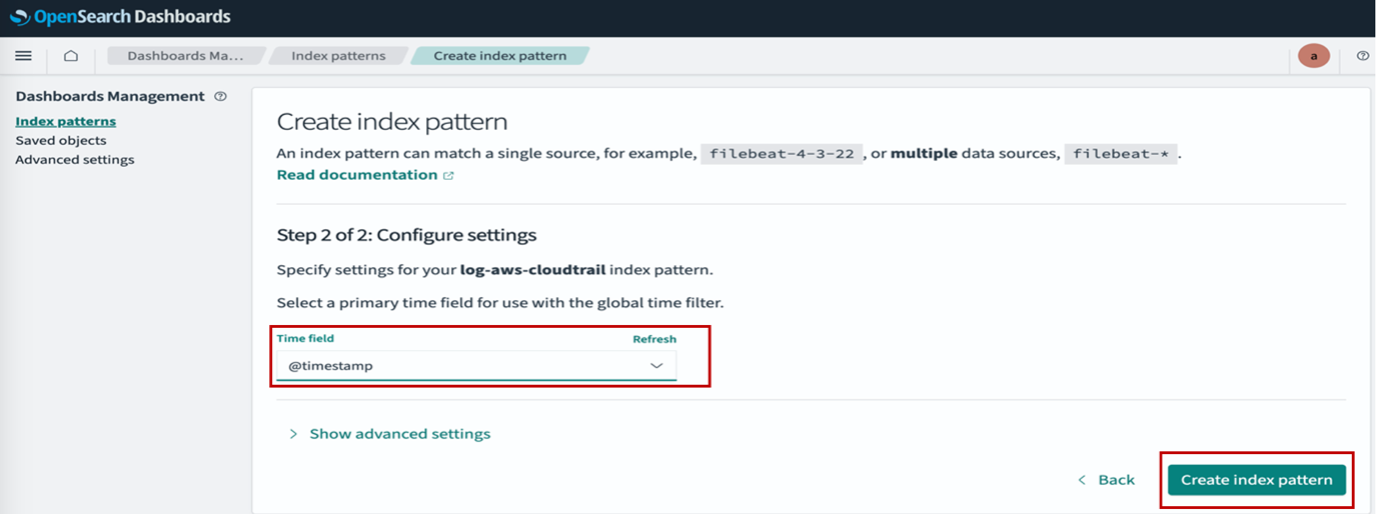
You must enable JWT authentication and authorization, and fine-grained access control during the OpenSearch Service domain creation process. For more information, refer to Configuring JWT authentication and authorization and Fine-grained access control in Amazon OpenSearch Service.
The following diagram illustrates the solution architecture.
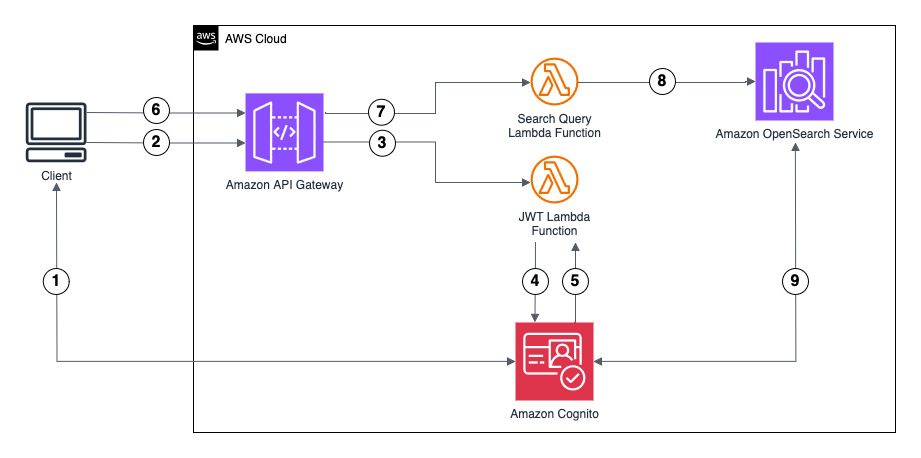
This solution demonstrates authentication using Amazon Cognito as the IdP to generate the JWT. However, you can use another supported IdP. The ID token includes group membership information that OpenSearch Service maps to roles configured using fine-grained access control.
The user flow consists of the following steps:
- The client initiates authentication by logging in with Amazon Cognito user credentials. Amazon Cognito returns an authorization code.
- The client sends the authorization code to an Amazon API Gateway /token endpoint for ID token exchange.
- API Gateway forwards the authorization code to an AWS Lambda function.
- The Lambda function sends a token exchange request to Amazon Cognito with the authorization code.
- The Lambda function receives the ID token from Amazon Cognito and returns it to the client.
- The client sends an OpenSearch Service query to the API Gateway /search endpoint, including the ID token. API Gateway validates the ID token (JWT) with Amazon Cognito.
- API Gateway forwards the request to a Lambda function.
- The Lambda function checks if JWT authentication and authorization is enabled for the OpenSearch Service domain with the respective public key of the Amazon Cognito user pool. If not, it will enable and configure this feature for the OpenSearch Service domain. The Lambda function forwards the query and ID token to OpenSearch Service.
- OpenSearch Service validates the JWT with Amazon Cognito:
- OpenSearch Service verifies user permissions against fine-grained access control based on group membership.
- OpenSearch Service returns query results to the client if authorization succeeds.
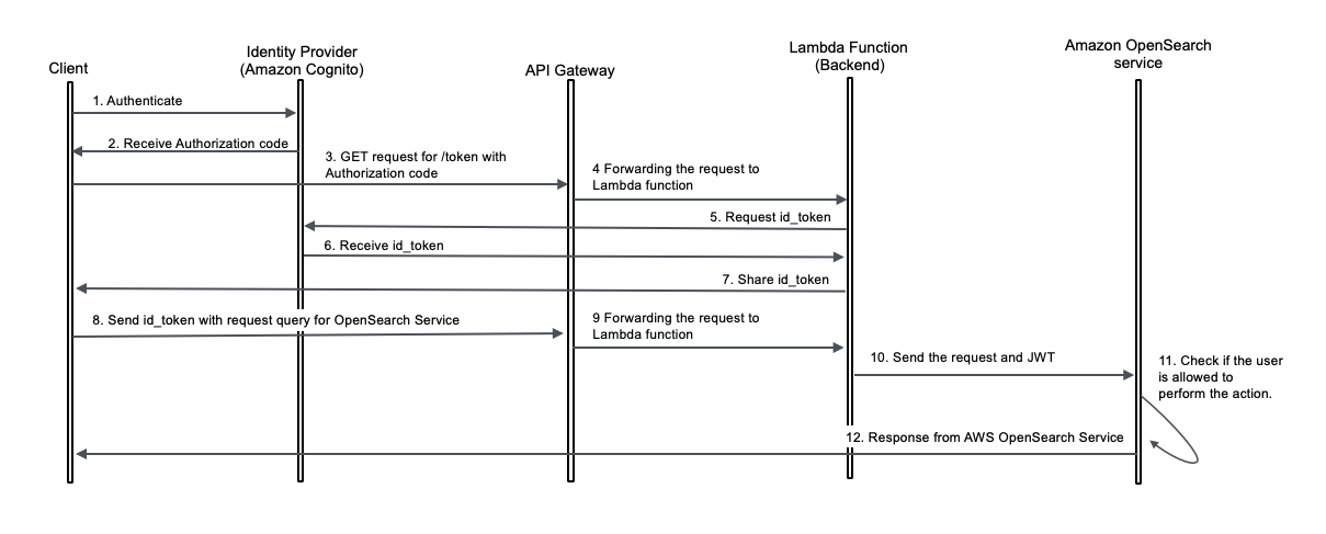
The following diagram illustrates the request flow.
Prerequisites
Before you deploy the solution, make sure you have the following prerequisites:
- An AWS account
- Familiarity with the Python programming language
- Familiarity with AWS Identity and Access Management (IAM) and OpenSearch Service
Deploy solution resources
To deploy the solution resources, we use an AWS CloudFormation template. Launch the AWS CloudFormation template with the following Launch Stack button.
![]()
Enter an appropriate stack name. This name is used as a prefix for resources like OpenSearch Service domains and Lambda functions. Keep the default settings, and choose Create.
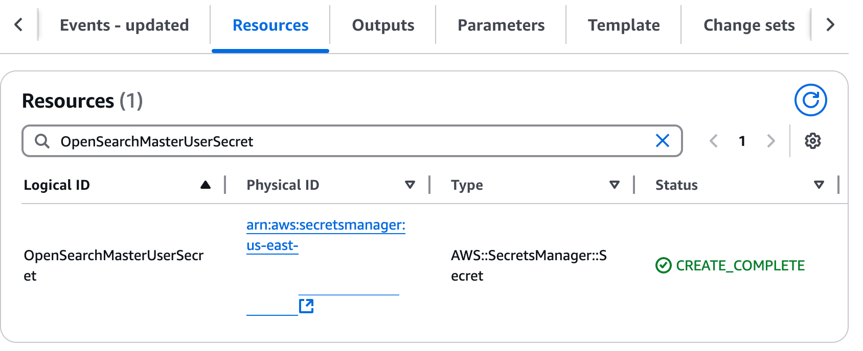
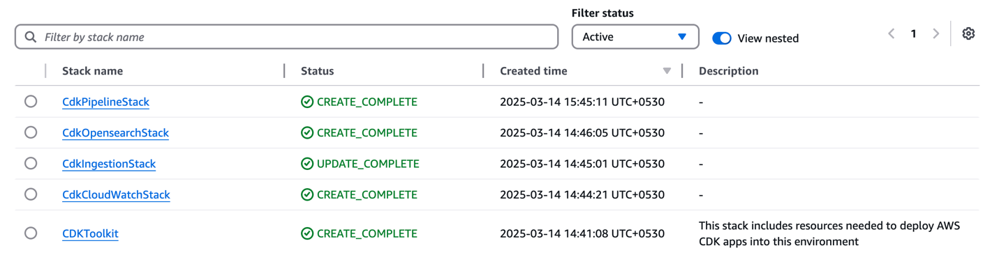
The stack deployment takes approximately 15–20 minutes. When deployment is complete, the stack status shows as CREATE_COMPLETE.
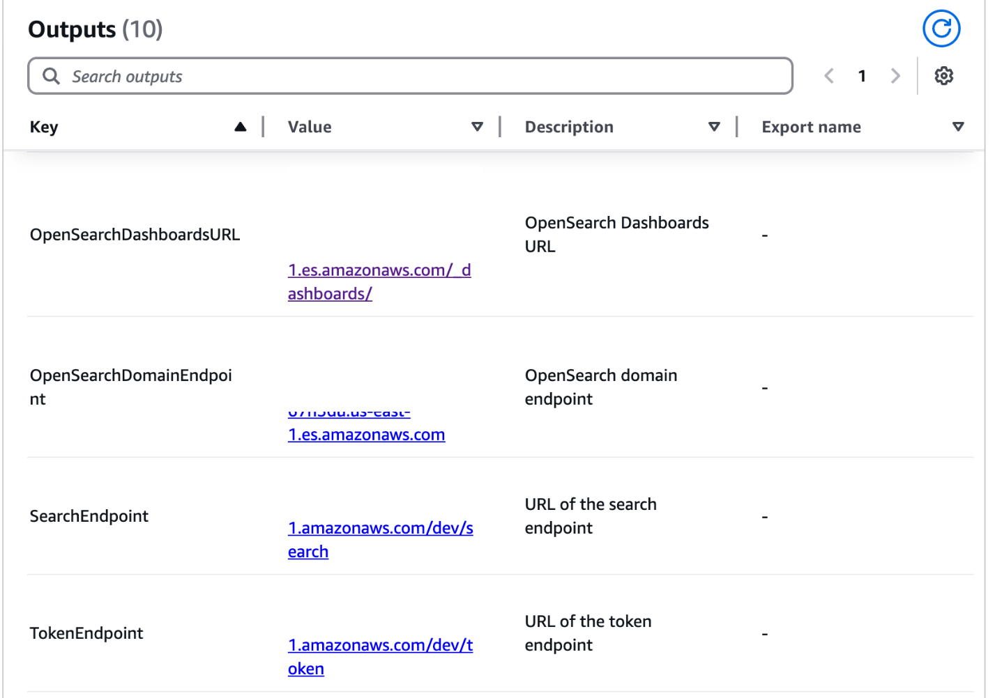
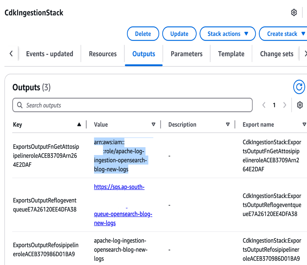
The outputs for this CloudFormation stack show important information regarding the deployed resources. This information will be referenced throughout different sections of this post.
On the Outputs tab, note the following values:
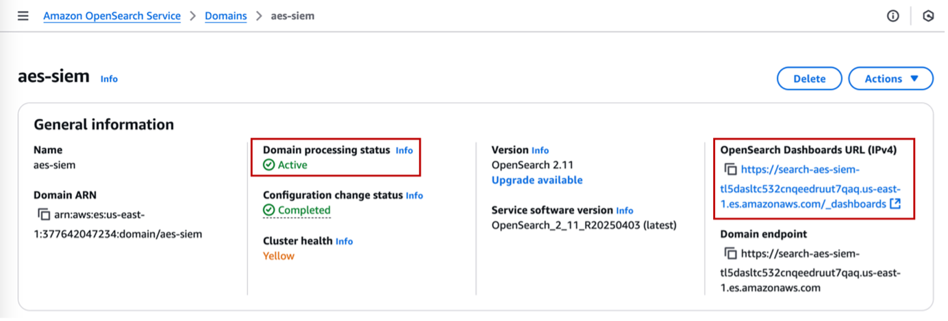
- OpenSearchDashboardURL
- SharedLambdaRoleArn
On the Resources tab, locate the following information:
- OpenSearchMasterUserSecret: Choose the Physical ID link, then choose Retrieve Secret Value. Note the user name and password required for OpenSearch Service domain login.
- IngestDataAndCreateBackendRoles: Choose the Physical ID link to open the Lambda function, needed in later steps.
- UserPool: Choose the Physical ID link to open the Amazon Cognito user pool, needed in later steps.
- RestAPI: Choose the Physical ID link to open the API Gateway endpoint, needed in later sections.
In a separate browser tab, log in to the OpenSearch dashboard using OpenSearchDashboardsURL and user credentials noted previously.
Assign permissions to the IAM role associated with the Lambda function
Complete the following steps to map your IAM role to both the all_access and security_manager roles in OpenSearch Service:
- In OpenSearch Dashboards, choose Security in the navigation pane, then choose Roles.
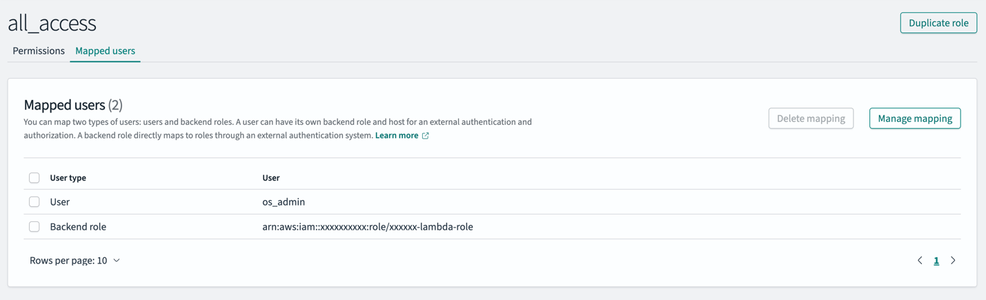
- Open the all_access role.
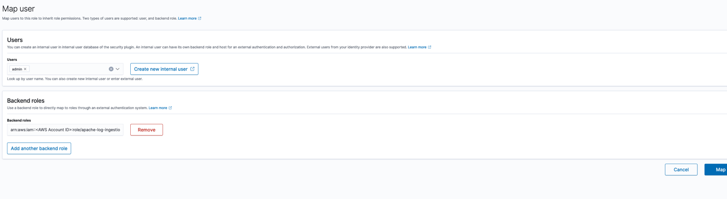
- In the Mapped users section, choose Manage mapping.
- For Backend role, enter the IAM role Amazon Resource name (ARN). This is the value you copied from the CloudFormation stack output for
SharedLambdaRoleArn. - Choose Map to confirm.
- On the Roles page, open the security_manager role.
- In the Mapped users section, choose Manage mapping.
- For Backend role, enter the same IAM role ARN.
- Choose Map to confirm the changes.
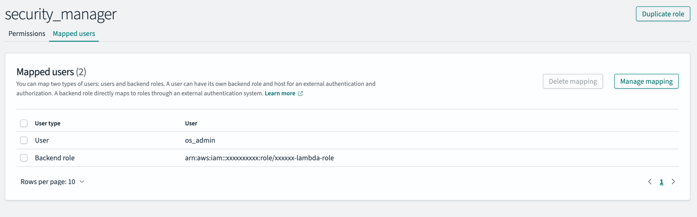
These steps ensure the IAM role attached to the Lambda function has the necessary permissions to ingest data (all_access) and create roles (security_manager) within the OpenSearch Service domain.
In this sample setup, the Lambda function handles bulk ingestion and role creation without granting any direct access to users, and all_access is provided to the Lambda role solely to enable ingestion. FGAC in OpenSearch provides in-depth access control, allowing you to further tighten the Lambda role permissions by granting only the necessary CRUD operations, rather than full access for ingestion. For more details, refer to Defining users and roles and Fine-grained access control in OpenSearch.
Run the Lambda function to ingest data into the OpenSearch Service domain
On the CloudFormation stack’s Resources tab, locate the IngestDataAndCreateBackendRoles Lambda function. Open the Lambda function, choose Test, and execute it. You can confirm the function’s successful execution by checking Amazon CloudWatch Logs.
This Lambda function is designed to perform bulk ingestion and role creation in the OpenSearch Service domain. It ingests sample clinical research data into OpenSearch Service, creating two indexes (pubmed and clinical_trials), and sets up required OpenSearch Service roles. We explore these roles in detail in the next section.
Map roles and users in OpenSearch Service
In this step, we define two key OpenSearch Service roles:
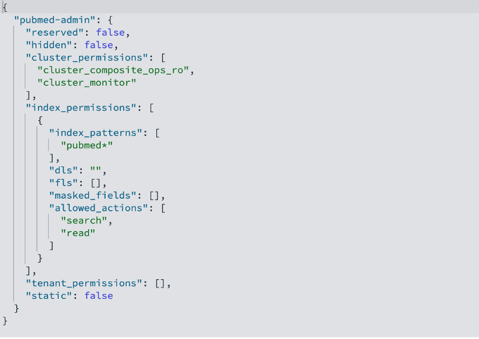
- pubmed-admin – Grants full read access to the PubMed index containing biomedical literature and research abstracts, intended for senior research groups
- pubmed-limited – Provides restricted read access to only specific fields (journal, title, and abstract, where journal is a masked field), intended for researchers with limited data access
We have already created these roles by running the Lambda function in the previous section. The following code is the pubmed-admin OpenSearch Service role description:
The following code is the pubmed-limited OpenSearch Service role description:
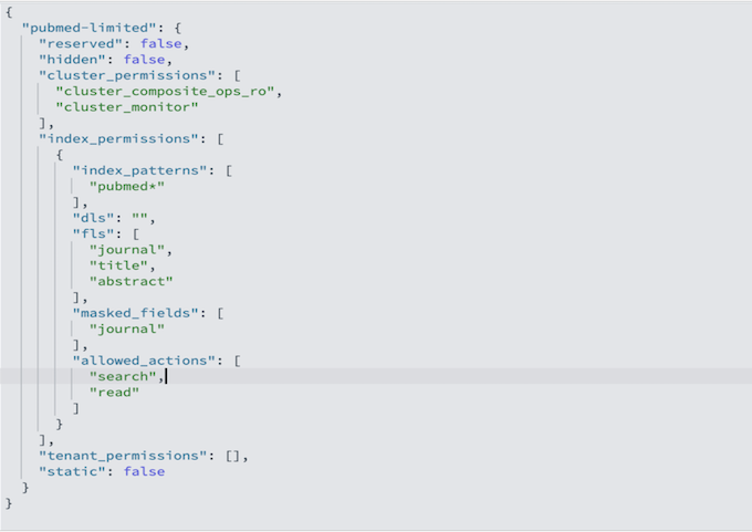
The pubmed-admin and pubmed-limited roles serve different purposes, and their main distinction lies in how they control data visibility. Document-level security (DLS) lets you restrict a role to a subset of documents in an index, while field-level security (FLS) lets you control which document fields a user can see. The limited role is configured with FLS to expose only the journal, title, and abstract fields, while masked fields anonymize sensitive data such as journal. On top of these, you can apply DLS to hide specific records, for example, to prevent users from viewing documents from certain journals or publication years. In your use cases, use DLS and FLS to control document and field visibility for different users. These roles are fully configurable; you can add, remove, or update document and field access at any time to match evolving security or business requirements.
To enforce access control, users need to be mapped to appropriate OpenSearch Service roles on OpenSearch Dashboards. Complete the following steps to map users to the OpenSearch Service roles:
- On OpenSearch Dashboards, choose Security in the navigation pane, then choose Roles.
- Open the
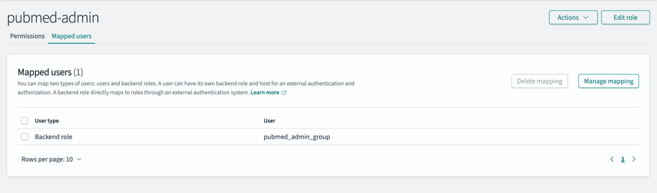
pubmed-adminrole. - In the Mapped users section, choose Manage mapping.
- For Backend role, enter
pubmed_admin_group. - Choose Map to confirm the mapping.
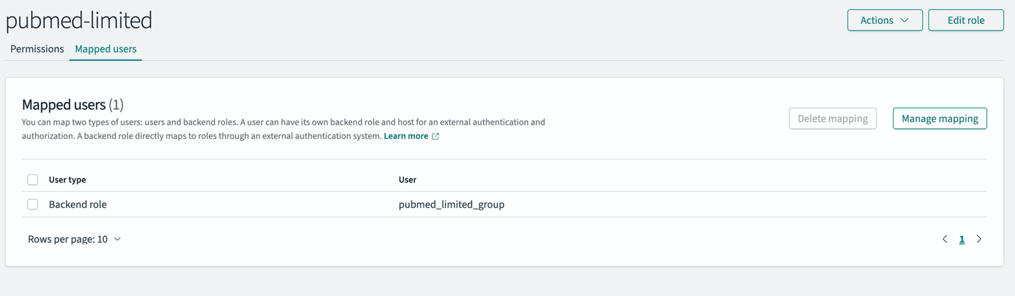
- On the Roles page, open the pubmed-limited role.
- In the Mapped users section, choose Manage mapping.
- For Backend role, enter pubmed_limited_group.
- Choose Map to confirm the mapping.
Backend roles simplify access management in OpenSearch Service. Instead of mapping individual users to OpenSearch service roles, you can map roles to backend roles that users share. This approach lets you map IdP groups directly to the OpenSearch service roles. OpenSearch Service provides options when configuring your OpenSearch Service domain to map JWT claims to OpenSearch Service roles using the roles key.
In this solution, the JWT contains a field called cognito:groups that will be mapped as the roles key. In every JWT, this field has a value for the appropriate group the user belongs to. Based on the field value in the JWT and the mapping defined in the previous step for different research groups, OpenSearch Service domain dynamically assigns permissions:
- If the JWT contains “cognito:groups”: [“pubmed_admin_group”], the user is granted pubmed_admin access
- If the JWT contains “cognito:groups”: [“pubmed_limited_group”], the user is granted pubmed_limited access
Take a look at the examples below to understand what a JWT header and payload look like.
Sample JWT header:
Sample JWT payload:
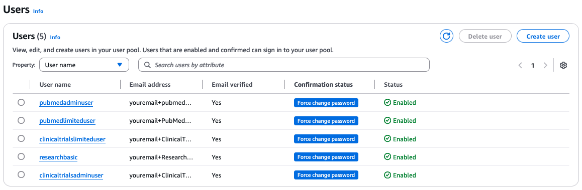
Create users in Amazon Cognito
In this section, we create the following Amazon Cognito users:
The email address required for each user should be unique. If your email domain supports email alias, you can add a suffix to your own email address by using [email protected]. The following screenshot shows our users.
On the CloudFormation stack’s Resources tab, locate the UserPool Amazon Cognito user pool that you noted earlier. Open the user pool in a new browser tab.
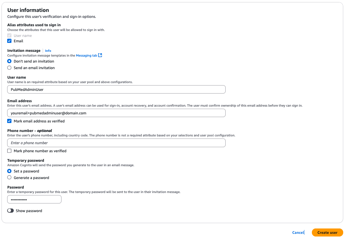
To create the Amazon Cognito users, complete the following steps for each user:
- On the Amazon Cognito console, choose Users in the navigation pane.
- Choose Create user.
- For Alias attributes used to sign in, select Email.
- For User name, enter a unique user name.
- For Email address, enter a unique email address for each user.
- Select Mark email address as verified.
- Choose Create User.
Create groups in Amazon Cognito
We create the following groups in Amazon Cognito:
The following screenshot shows created groups.
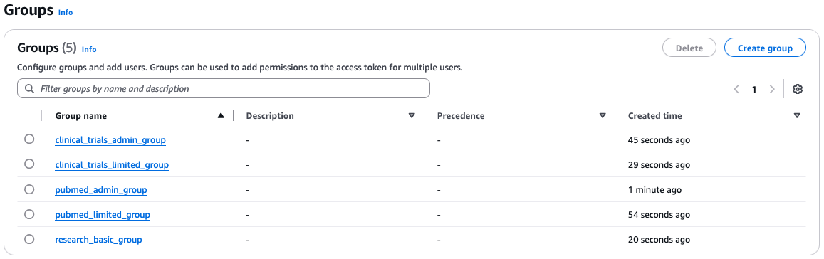
To create the Amazon Cognito groups, complete the following steps for each group:
- On the Amazon Cognito console, choose Groups in the navigation pane.
- Choose Create group.
- For Group name, enter a unique name.
- Choose Create group.
Add Amazon Cognito users to groups
The users should be added to the groups as follows:
- Add
PubMedAdminUserto thepubmed_admin_groupgroup - Add
PubMedLimitedUserto thepubmed_limited_groupgroup - Add
ClinicalTrialsAdminUserto theclinical_trials_admin_groupgroup - Add
ClinicalTrialsLimitedUserto theclinical_trials_limited_groupgroup - Add
ResearchBasicUserto theresearch_basic_groupgroup
To add users to their respective group, complete the following steps for each group:
- On the Amazon Cognito console, choose Groups in the navigation pane.
- Choose the group to which you want to add a user.
- Choose Add user to group.
- Choose the user and choose Add.
Log in to generate a JWT
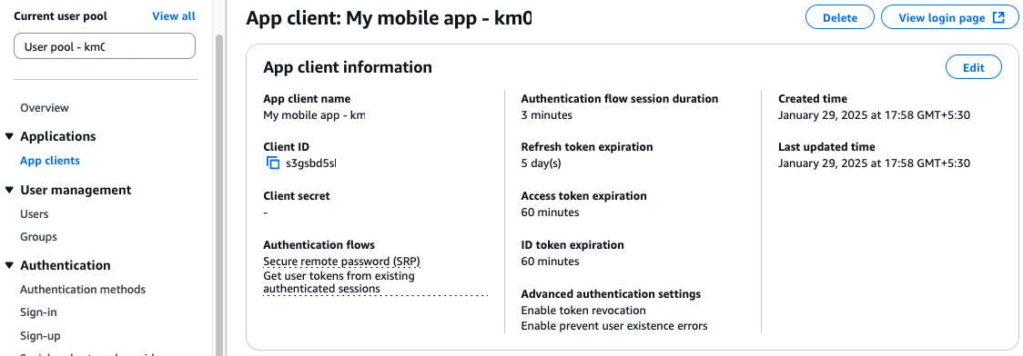
Before running the test queries in the next section, you must obtain the id_token (JWT) for the specified users. The tokens will expire in 60 minutes. If the token is expired for a user, you must log in again to get a fresh token. To log in with your user to get the id_token, complete the following steps:
- On the Amazon Cognito console, open your user pool.
- Choose App clients in the navigation pane.
- Choose the app client.
- Choose View login page.
- Enter the user name that you used when creating the user.
- Enter the temporary password that you set when creating the user.
- For first-time logins, you will be prompted to create a new password. Enter a new password that meets the following requirements:
- At least 8 characters
- Contains uppercase and lowercase letters
- Contains at least one number
- Contains at least one special character
- Copy the id_token value you generated (without quotation marks).
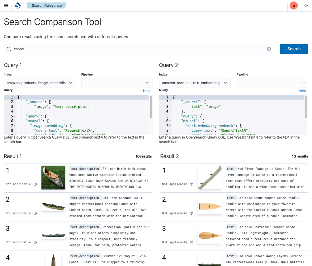
Query data in OpenSearch Service
This example demonstrates how OpenSearch Service filters search results based on user permissions. We test searches using JWTs for two different users to verify access controls. Each user’s search results are limited to the indexes and documents allowed by their assigned roles.
On the CloudFormation stack’s Resources tab, locate the RestAPI value that you noted earlier. Open the API gateway in a new browser tab.
Complete the following steps to test the search API for each of the scenarios mentioned in this section:
- On the API Gateway console, choose Resources in the navigation pane.
- Choose the /search resource.
- Choose the POST method.
- Choose Test.
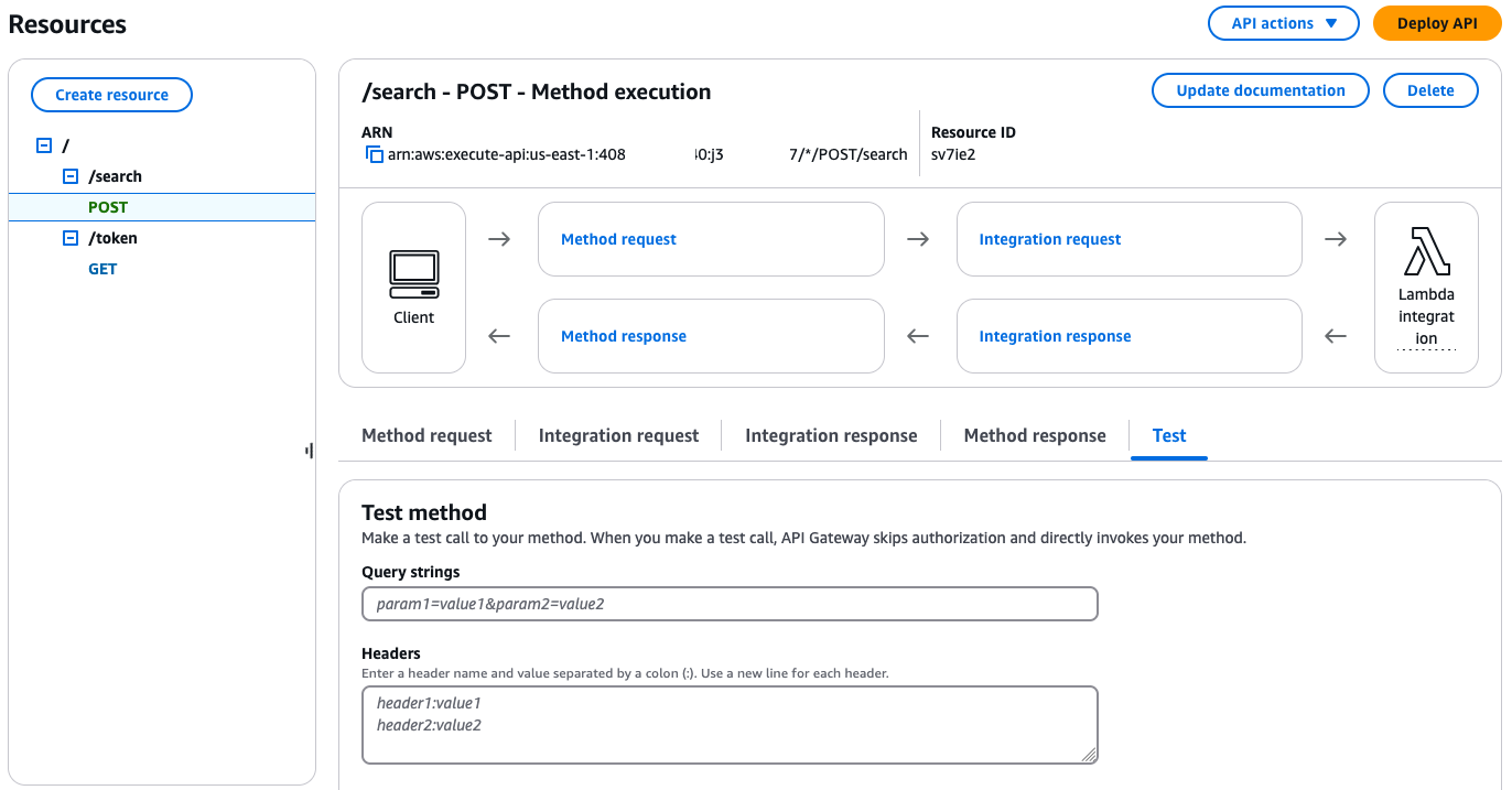
When submitting queries to OpenSearch Service, make sure all double quotation marks are escaped to prevent syntax errors. Additionally, make sure you complete your query before your JWT expires, or you will need to generate a new token. If you attempt to use an expired token, it will result in an error.
For Scenarios 1 and 2, log in with your PubMedAdmin user, and for Scenarios 3 and 4, log in with your PubMedLimitedUser to obtain the required id_token.
Scenario 1
In this first query, we query the pubmed index with the credentials of user PubMedAdminUser, which is part of pubmed_admin_group:
Add the following values to the respective input fields:
- For Query strings, enter query=
"{\"query\":{\"match_all\":{}}}"&index=pubmed - For Headers, enter id_token:<id-token-for-PubMedAdminUser>
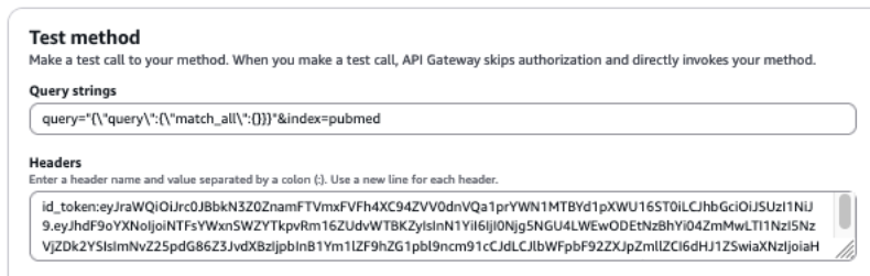
The following screenshot shows our query results.
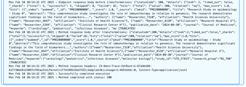
Users with the pubmed_admin role have full access to the PubMed index and can perform unrestricted searches across all fields and document types. This query successfully returns documents with the HTTP 200 status code because the user has complete read permissions on this index.
Scenario 2
Next, we query the clinical-trials index with the credentials of user PubMedAdminUser, who is part of pubmed_admin_group:
Add the following values to the respective input fields:
- For Query strings, enter query=
"{\"query\":{\"match_all\":{}}}"&index=clinical-trials - For Headers, enter
id_token:<id-token-for-PubMedAdminUser>
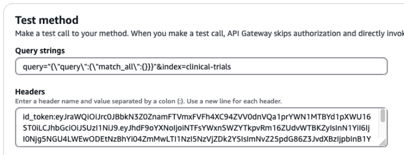
The following screenshot shows our query results.
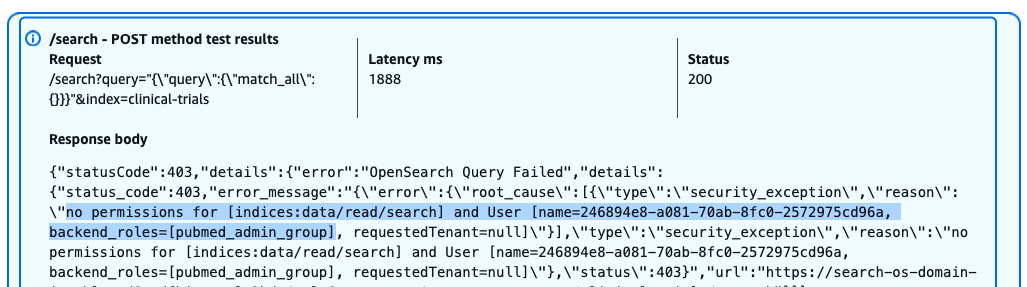
Despite having admin privileges for PubMed data, this user receives a 403 Forbidden response when attempting to access the clinical-trials index. The error message indicates the lack of necessary permissions for performing search operations on this index.
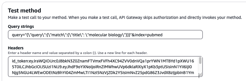
Scenario 3
Now we query allowed fields in the pubmed index with the credentials of user PubMedLimitedUser, which is part of pubmed_limited_group:
Add the following values to the respective input fields:
- For Query strings, enter query=
"{\"query\":{\"match\":{\"title\": \"molecular biology\"}}}"&index=pubmed - For Headers, enter
id_token:<id-token-for-PubMedLimitedUser>
The following screenshot shows our query results.
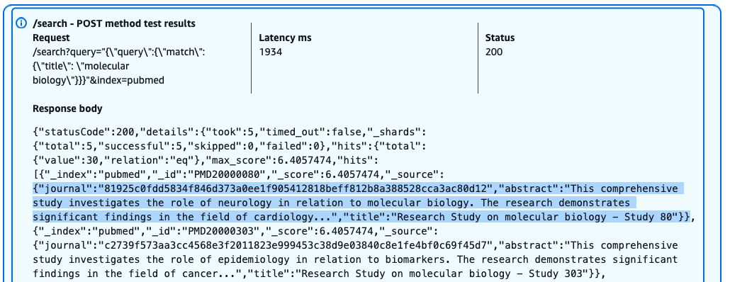
Users with the pubmed_limited role can successfully query specific fields like title, but with restricted access to sensitive information. The query returns results with the HTTP 200 status code, but the journal field is anonymized due to field-level security policies. Users can search and view certain fields while having sensitive data automatically masked or excluded from their results.
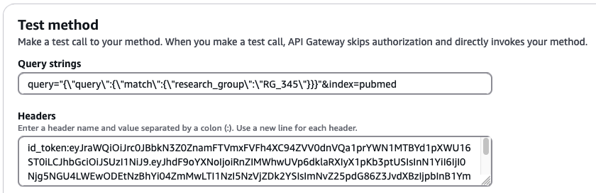
Scenario 4
Lastly, we query unauthorized fields in the pubmed index with the credentials of user PubMedLimitedUser, which is part of pubmed_limited_group:
Add the following values to the respective input fields:
- For Query strings, enter query=
"{\"query\":{\"match\":{\"research_group\":\"RG_345\"}}}"&index=pubmed - For Headers, enter
id_token:<id-token-for-PubMedLimitedUser>
The following screenshot shows our query results.
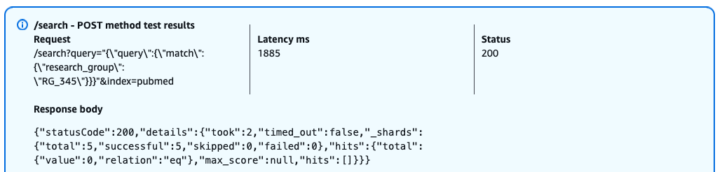
When a user with the pubmed_limited role attempts to query the restricted research_group field, OpenSearch returns a successful response (HTTP 200) but with empty results. This behavior occurs because field-level security is enforcing access controls instead of returning a HTTP 403 error, it silently filters out the restricted field from both the query and results. This security-by-obscurity approach means that users can’t determine whether their query failed due to lack of permissions or genuine absence of matching documents.
Clean up
To avoid incurring further AWS usage charges, delete the resources created in this post by deleting the CloudFormation stack. This step will remove all resources except Lambda layers. To delete the Lambda layers, navigate to the Layers page on the Lambda console, and delete the layers named <CloudFormation-Stack-Name>-requests and <CloudFormation-Stack-Name>-crypt.
Conclusion
In this post, we discussed how JWTs provide a robust and scalable authentication mechanism that can be integrated with existing IdPs. We also demonstrated how to seamlessly integrate fine-grained access control across search applications. Organizations can define granular permissions within their IdP, making sure sensitive information remains protected. The JWT integration with OpenSearch Service enables secure, efficient access control, so users can only access role-appropriate information while simplifying compliance and access management.
If you have feedback about this post, leave them in the comments section. If you have questions about this post, start a new thread on AWS Security, Identity, and Compliance re:Post or contact AWS Support.
About the authors
 Ramya Bhat is a Data Analytics Consultant at AWS, specializing in the design and implementation of cloud-based data platforms. She builds enterprise-grade solutions across search, data warehousing, and ETL that enable organizations to modernize data ecosystems and derive insights through scalable analytics. She has delivered customer engagements across healthcare, insurance, fintech, and media sectors.
 Shubhansu Sawaria is a Sr. Delivery Consultant – SRC at AWS, based in Bangalore, India. He specializes in designing and implementing comprehensive AWS Cloud security solutions. He has developed security solutions for startups, banks, and healthcare organizations. His expertise helps organizations elevate their cloud security infrastructures, achieve compliance objectives, and provide robust data protection.
 Soujanya Konka is a Sr. Solutions Architect and Analytics Specialist at AWS, focused on helping customers build their ideas in the cloud. She has expertise in designing and implementing enterprise search solutions and advanced data analytics at scale.


 Smita Singh is a Senior Solutions Architect at AWS. She focuses on defining technical strategic vision and works on architecture, design, and implementation of modern, scalable platforms for large-scale global enterprises and SaaS providers. She is a data, analytics, and generative AI enthusiast and is passionate about building innovative, highly scalable, resilient, fault-tolerant, self-healing, multi-tenant platform solutions and accelerators.
 Dipayan Sarkar is a Specialist Solutions Architect for Analytics at AWS, where he helps customers modernize their data platform using AWS analytics services. He works with customers to design and build analytics solutions, enabling businesses to make data-driven decisions.


 Kunal Kotwani is a software engineer at Amazon Web Services, focusing on OpenSearch core and vector search technologies. His major contributions include developing storage optimization solutions for both local and remote storage systems that help customers run their search workloads more cost-effectively.
 Navneet Verma is a senior software engineer at AWS OpenSearch . His primary interests include machine learning, search engines and improving search relevancy. Outside of work, he enjoys playing badminton.
 Sorabh Hamirwasia is a senior software engineer at AWS working on the OpenSearch Project. His primary interest include building cost optimized and performant distributed systems.


 Ravikiran Rao is a Data Architect at Amazon Web Services and is passionate about solving complex data challenges for various customers. Outside of work, he is a theater enthusiast and amateur tennis player.
 Vishwa Gupta is a Senior Data Architect with the AWS Professional Services Analytics Practice. He helps customers implement big data and analytics solutions. Outside of work, he enjoys spending time with family, traveling, and trying new food.
 Suvojit Dasgupta is a Principal Data Architect at Amazon Web Services. He leads a team of skilled engineers in designing and building scalable data solutions for AWS customers. He specializes in developing and implementing innovative data architectures to address complex business challenges.This post showcases how to use Spark on AWS Glue to seamlessly ingest data into OpenSearch Service. We cover batch ingestion methods, share practical examples, and discuss best practices to help you build optimized and scalable data pipelines on AWS.
 Aruna Govindaraju is an Amazon OpenSearch Specialist Solutions Architect and has worked with many commercial and open-source search engines. She is passionate about search, relevancy, and user experience. Her expertise with correlating end-user signals with search engine behavior has helped many customers improve their search experience.
 Vamshi Vijay Nakkirtha is a software engineering manager working on the OpenSearch Project and Amazon OpenSearch Service. His primary interests include distributed systems. He is an active contributor to various OpenSearch projects such as k-NN, Geospatial, and dashboard-maps.


 Nikhil Agarwal is a Sr. Technical Manager with Amazon Web Services. He is passionate about helping customers achieve operational excellence in their cloud journey and actively working on technical solutions. He is an artificial intelligence (AI/ML) and analytics enthusiastic, he deep dives into customer’s ML and OpenSearch service specific use cases. Outside of work, he enjoys traveling with family and exploring different gadgets.
 Rick Balwani is an Enterprise Support Manager responsible for leading a team of Technical Account Mangers (TAMs) supporting AWS independent software vendor (ISV) customers. He works to ensure customers are successful on AWS and can build cutting-edge solutions. Rick has a background in DevOps and system engineering.
 Ashwin Barve is a Sr. Technical Manager with Amazon Web Services. In his role, Ashwin leverages his experience to help customers align their workloads with AWS best practices and optimize resources for maximum cost savings. Ashwin is dedicated to assisting customers through every phase of their cloud adoption, from accelerating migrations to modernizing workloads.

 Balaji Mohan is a senior modernization architect specializing in application and data modernization to the cloud. His business-first approach ensures seamless transitions, aligning technology with organizational goals. Using cloud-native architectures, he delivers scalable, agile, and cost-effective solutions, driving innovation and growth.
 Souvik Bose is a Software Development Engineer working on Amazon OpenSearch Service.
 Muthu Pitchaimani is a Search Specialist with Amazon OpenSearch Service. He builds large-scale search applications and solutions. Muthu is interested in the topics of networking and security, and is based out of Austin, Texas.

 Aswath Srinivasan is a Senior Search Engine Architect at Amazon Web Services currently based in Munich, Germany. With over 17 years of experience in various search technologies, Aswath currently focuses on OpenSearch. He is a search and open-source enthusiast and helps customers and the search community with their search problems.
 Jon Handler is a Senior Principal Solutions Architect at Amazon Web Services based in Palo Alto, CA. Jon works closely with OpenSearch and Amazon OpenSearch Service, providing help and guidance to a broad range of customers who have search and log analytics workloads that they want to move to the AWS Cloud. Prior to joining AWS, Jon’s career as a software developer included 4 years of coding a large-scale, ecommerce search engine. Jon holds a Bachelor of the Arts from the University of Pennsylvania, and a Master of Science and a PhD in Computer Science and Artificial Intelligence from Northwestern University.


 Ayush Agrawal is a Startups Solutions Architect from Gurugram, India with 11 years of experience in Cloud Computing. With a keen interest in AI, ML, and Cloud Security, Ayush is dedicated to helping startups navigate and solve complex architectural challenges. His passion for technology drives him to constantly explore new tools and innovations. When he’s not architecting solutions, you’ll find Ayush diving into the latest tech trends, always eager to push the boundaries of what’s possible.
 Fraser Sequeira is a Solutions Architect with AWS based in Mumbai, India. In his role at AWS, Fraser works closely with startups to design and build cloud-native solutions on AWS, with a focus on analytics and streaming workloads. With over 10 years of experience in cloud computing, Fraser has deep expertise in big data, real-time analytics, and building event-driven architecture on AWS.


 Arun Lakshmanan is a Search Specialist with Amazon OpenSearch Service based out of Chicago, IL. He has over 20 years of experience working with enterprise customers and startups. He loves to travel and spend quality time with his family.
 Madhan Kumar Baskaran works as a Search Engineer at AWS, specializing in Amazon OpenSearch Service. His primary focus involves assisting customers in constructing scalable search applications and analytics solutions. Based in Bengaluru, India, Madhan has a keen interest in data engineering and DevOps.


 Michael Hamilton is a Sr Analytics Solutions Architect focusing on helping enterprise customers modernize and simplify their analytics workloads on AWS. He enjoys mountain biking and spending time with his wife and three children when not working.
 Daniel Rozo is a Senior Solutions Architect with AWS supporting customers in the Netherlands. His passion is engineering simple data and analytics solutions and helping customers move to modern data architectures. Outside of work, he enjoys playing tennis and biking.
 Stavros Macrakis is a Senior Technical Product Manager on the OpenSearch project of Amazon Web Services. He is passionate about giving customers the tools to improve the quality of their search results.


 Jack Mazanec is a software engineer working on OpenSearch plugins. His primary interests include machine learning and search engines. Outside of work, he enjoys skiing and watching sports.
 Othmane Hamzaoui is a Data Scientist working at AWS. He is passionate about solving customer challenges using Machine Learning, with a focus on bridging the gap between research and business to achieve impactful outcomes. In his spare time, he enjoys running and discovering new coffee shops in the beautiful city of Paris.