All posts by Gaurav Sharma

Building medallion architecture with Iceberg materialized views in Amazon SageMaker

Post Syndicated from Gaurav Sharma original https://aws.amazon.com/blogs/big-data/building-medallion-architecture-with-iceberg-materialized-views-in-amazon-sagemaker/

Building a Medallion Architecture today typically means that you must build three separate systems working in concert: extract, transform, and load (ETL) jobs to transform data between layers, an orchestrator (such as Apache Airflow or AWS Step Functions) to sequence those jobs in the correct order, and custom change-data-capture (CDC) logic to make sure that each job processes only new or modified records. Each component must be authored, tested, deployed, and maintained independently and when one breaks, the entire pipeline stalls.

In this post, we show how Apache Iceberg materialized views in Amazon SageMaker collapse transformation, orchestration, and incremental processing into a single SQL definition per layer. You declare what each layer should contain, and the system handles when and how it refreshes based on your refresh configuration. With this approach, you can build a Bronze → Silver → Gold pipeline with three SQL statements. This reduces the complexity of maintaining separate orchestration code, CDC logic, and job artifacts.

What is medallion architecture

The medallion architecture organizes data into three progressive layers:

  • Bronze layer – Captures raw data as-is from source systems, preserving the original format for auditability and replay.
  • Silver layer – Applies cleaning, deduplication, type casting, and business logic to produce validated, query-ready datasets.
  • Gold layer – Aggregates Silver data into business-level metrics, key performance indicators (KPIs), and dimensional models optimized for analytics and reporting.

Each layer builds on the previous one, creating clear lineage from raw ingestion to business insight.

Traditional versus declarative approach

The two approaches differ in how much infrastructure you build and maintain.

Traditional approach

You write an ETL job such as Apache Spark script for Bronze to Silver layer and another for Silver to Gold layer. You build a directed acyclic graph (DAG) in Apache Airflow or a Step Functions state machine to run them in order. You implement CDC logic like tracking high watermarks, comparing snapshots, or consuming change streams such that each job processes only new data.

Declarative approach with Iceberg materialized views

You write one CREATE MATERIALIZED VIEW statement per layer with a SCHEDULE REFRESH EVERY N HOURS clause. The AWS Glue managed Spark compute executes the refresh, but you don’t author, version, or deploy a job artifact. Iceberg’s row-level change tracking (position-delete and equality-delete files) identifies which rows changed since the last refresh and AWS Glue processes only those rows. The dependency chain is implicit in the SQL definitions. The only code you maintain is the SQL transformation logic itself.

Apache Iceberg and materialized views

Apache Iceberg is an open-source, high-performance table format designed for petabyte-scale analytic datasets in data lakes. It provides ACID transactions, time travel, schema evolution, and hidden partitioning.

With an Iceberg materialized view, you can define each layer of a medallion architecture as a SQL statement. Under the hood, AWS Glue uses Iceberg’s change-tracking metadata to identify which rows changed since the last refresh, then processes only those rows using managed Spark compute. You configure scheduling and incremental processing through SQL definitions, and the system executes atomic refreshes without requiring you to write pipeline code.

When refreshed, the Gold materialized view reads incrementally from the Silver materialized view, which in turn reads from the Bronze table. This creates a declarative dependency chain: each layer’s definition points to the layer below it, and the system resolves which data to reprocess at each refresh.

Service support for Iceberg materialized views

At time of publication, the following services support creating and refreshing Iceberg materialized views:

For the latest version requirements, see the AWS Glue materialized views documentation.

Technical architecture

The architecture uses Amazon S3 Tables, a capability of Amazon Simple Storage Service (Amazon S3), as the storage layer. Amazon S3 Tables is a managed Apache Iceberg offering that alleviates the administrative overhead of maintaining Iceberg tables. AWS Glue Data Catalog manages table metadata, and Amazon SageMaker Unified Studio provides the AI-powered notebook environment with AWS Glue 5.1 for authoring and executing materialized view definitions.

The diagram illustrates a three-tier data lakehouse pipeline built on Apache Iceberg. The Bronze layer contains raw trip data (trips_bronze table on S3 Tables with fields: trip_id, city, vehicle_type, fare, status) that you ingest through INSERT/Append operations.

An incremental REFRESH feeds the Silver layer, where a materialized view (mv_trips_silver) performs timestamp conversion, null filtering, and computes derived columns like revenue_per_mile and rating_category. It processes only new or changed rows.

The Silver layer then refreshes two Gold layer materialized views on a daily schedule: mv_city_daily_metrics (city, date, trips, drivers, revenue, tips) and mv_vehicle_performance (vehicle_type, city, trips, revenue, distance). The Gold layer serves downstream consumers including Amazon Athena, Amazon Quick Sight, Amazon Redshift, and first-party (1P) or third-party (3P) compute engines supporting the Iceberg REST API.

The pipeline flows as follows:
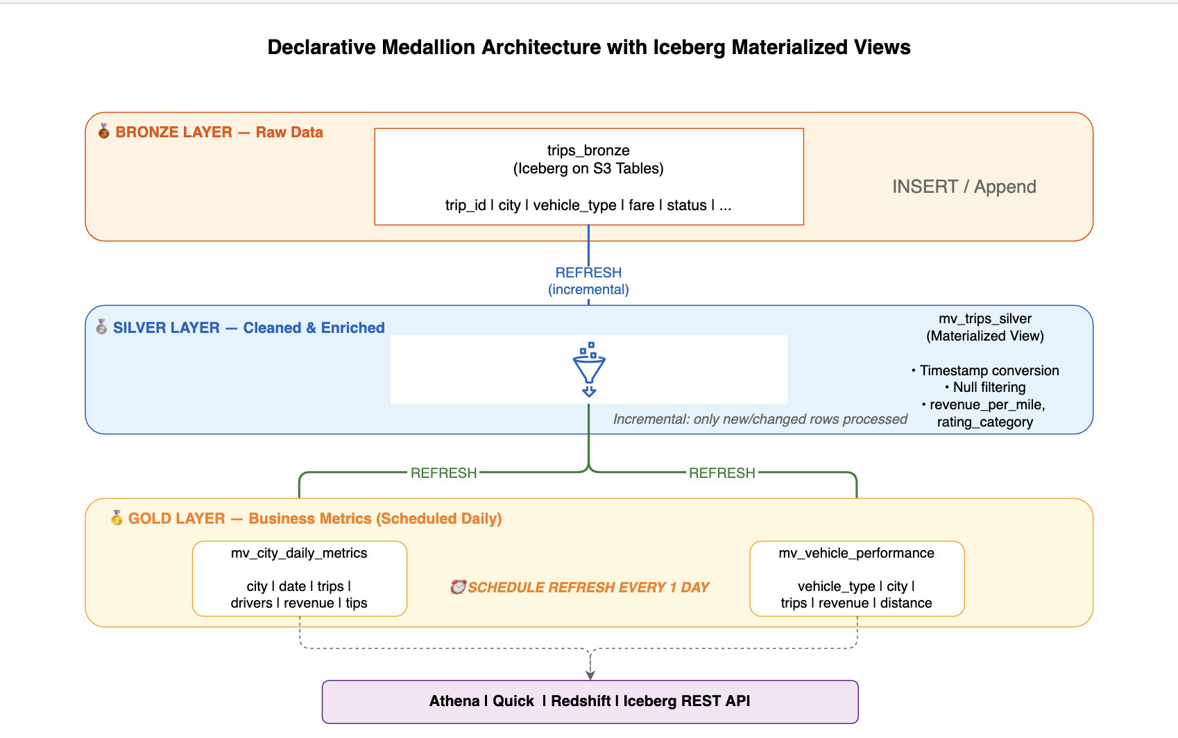
Diagram of the medallion pipeline: a Bronze table feeds a Silver materialized view that feeds two Gold materialized views consumed by analytics engines

Figure 1: The three-tier medallion pipeline from the Bronze table through Silver and Gold materialized views to analytics consumers

Prerequisites

Before starting, verify that you have the following:

  • An AWS account with permissions for Amazon SageMaker Unified Studio, AWS Glue, S3 Tables, and AWS Lake Formation.
  • An Amazon SageMaker Unified Studio domain.

Step 1: Initialize the environment

Open the AWS Management Console and navigate to Amazon SageMaker.
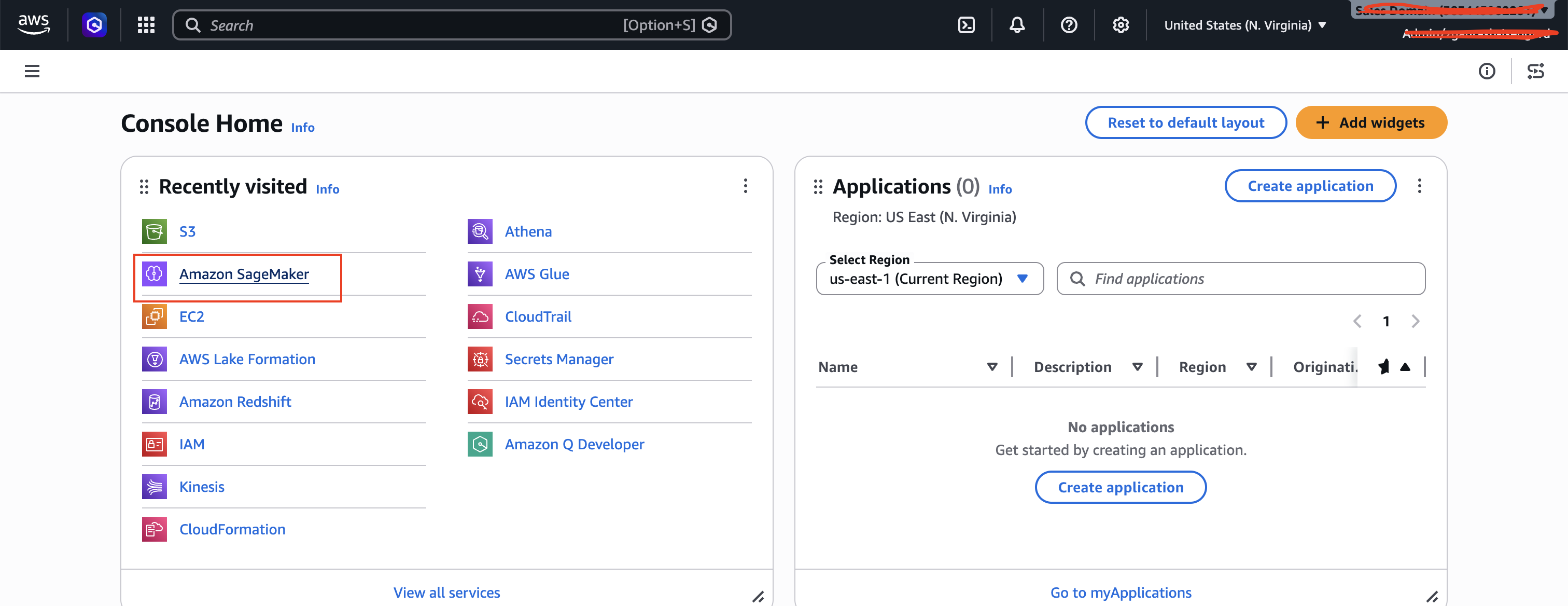
Amazon SageMaker console landing page

Figure 2: The Amazon SageMaker console landing page

Choose Get Started to set up Amazon SageMaker Unified Studio.
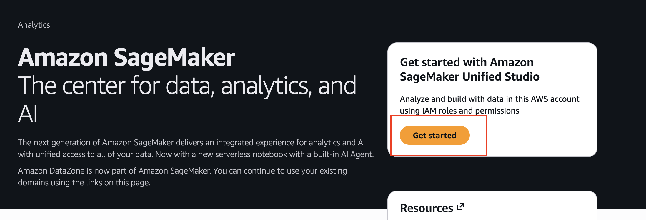
SageMaker Unified Studio Get Started setup page

Figure 3: The Get Started page for setting up SageMaker Unified Studio

Choose Open to launch Amazon SageMaker Unified Studio.
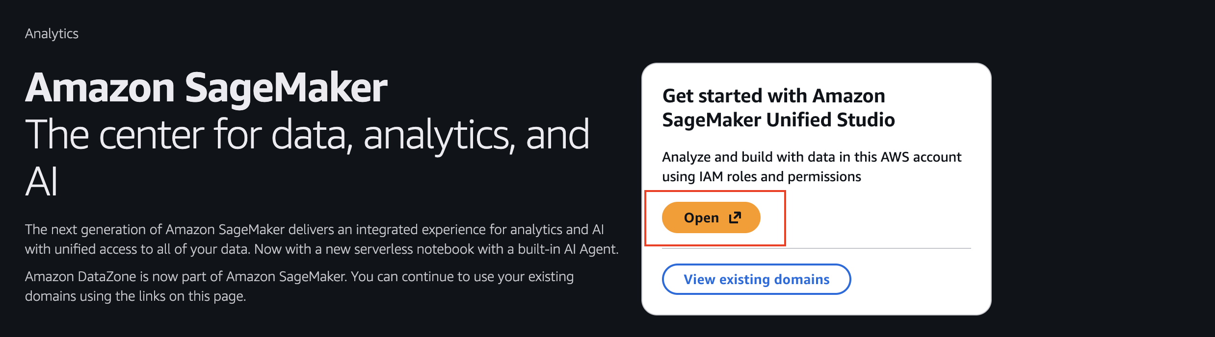
Button to open and launch SageMaker Unified Studio

Figure 4: The option to open and launch SageMaker Unified Studio

After you’re in SageMaker Unified Studio, choose Data in the left pane to create the S3 Tables bucket (a managed Apache Iceberg feature of Amazon S3) and a database. Choose Add, then choose Create S3 Tables Catalog, and provide a catalog and a database name. Finally, choose Create Catalog.
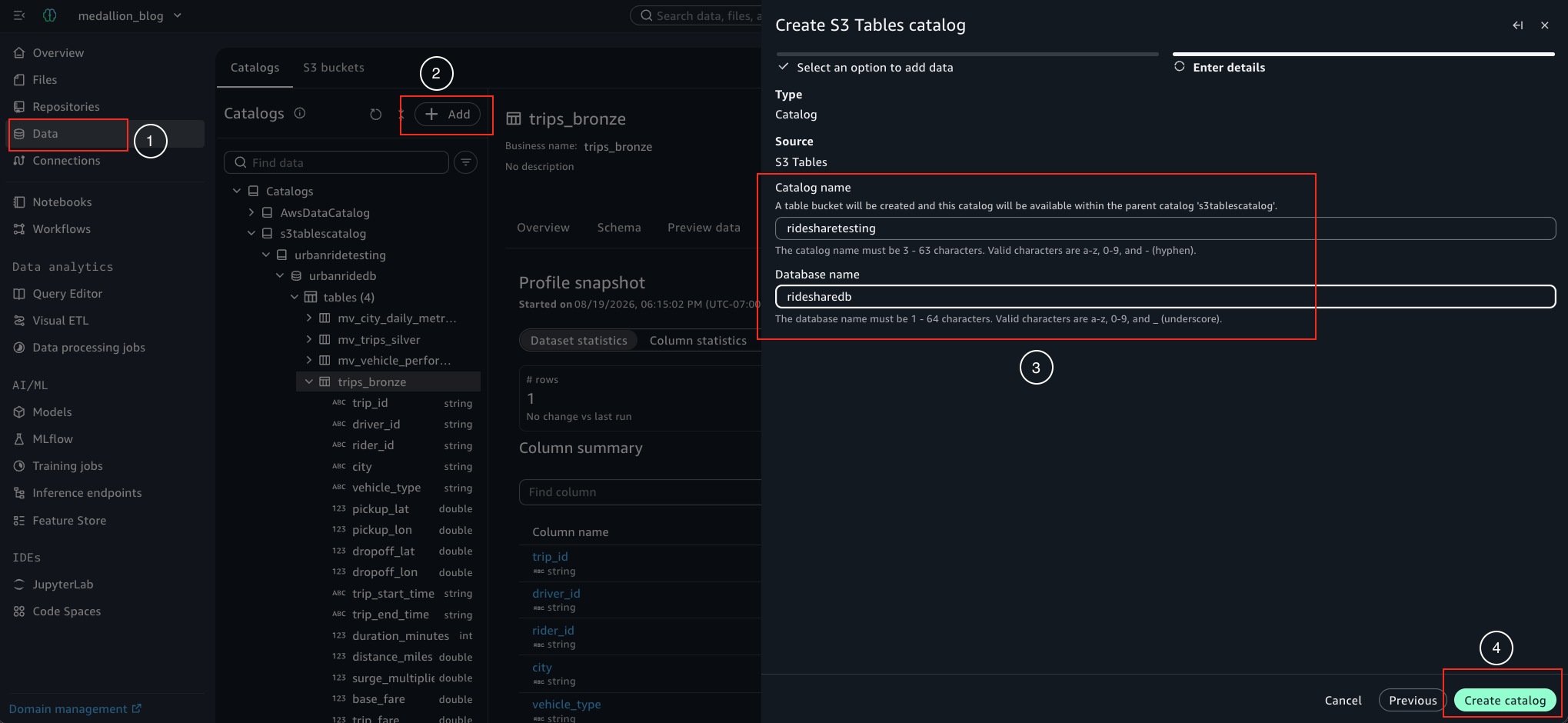
Create S3 Tables Catalog dialog with catalog and database name fields

Figure 5: The Create S3 Tables Catalog dialog with catalog and database name fields

After the catalog creation is complete, in the left navigation pane, choose Notebooks.
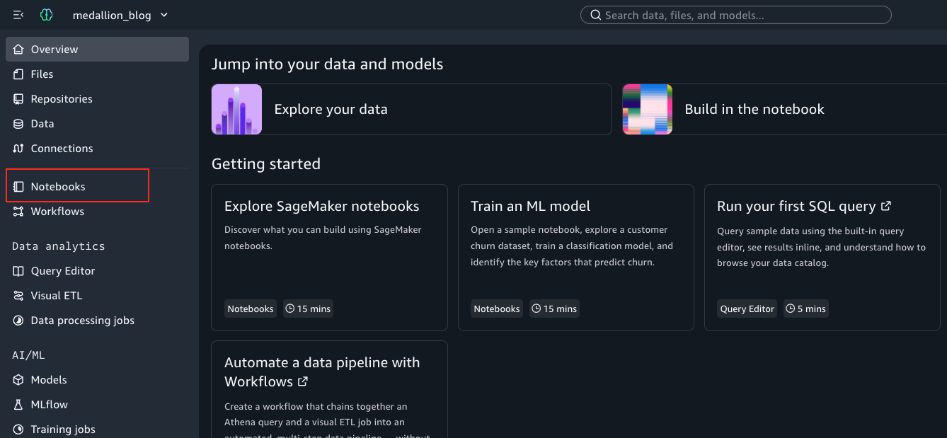
Notebooks option in the SageMaker Unified Studio left navigation pane

Figure 6: The Notebooks option in the SageMaker Unified Studio navigation pane

Choose Create Notebook.
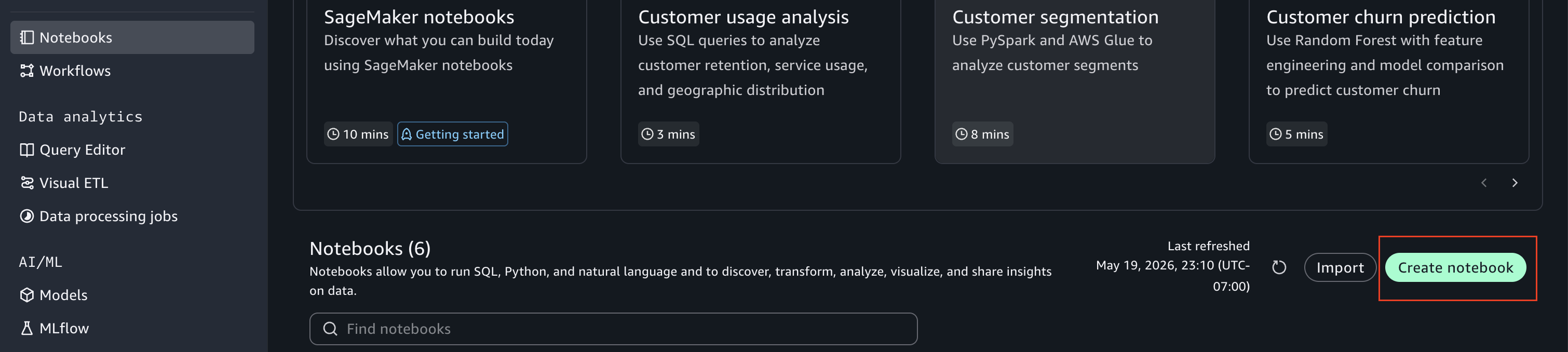
Create Notebook button in SageMaker Unified Studio

Figure 7: The Create Notebook button in SageMaker Unified Studio

Before using the notebook, select either Athena Spark or Glue Spark compute connection as the runtime engine for your notebook.
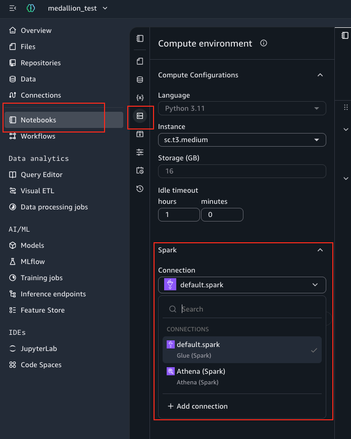
Runtime engine selection showing Athena Spark and Glue Spark compute connections

Figure 8: Selecting Athena Spark or Glue Spark as the notebook runtime engine

Use the following code samples in individual notebook cells. You can also provide transformation requirements in natural language, and the SageMaker Data Agent will generate SQL code for you.
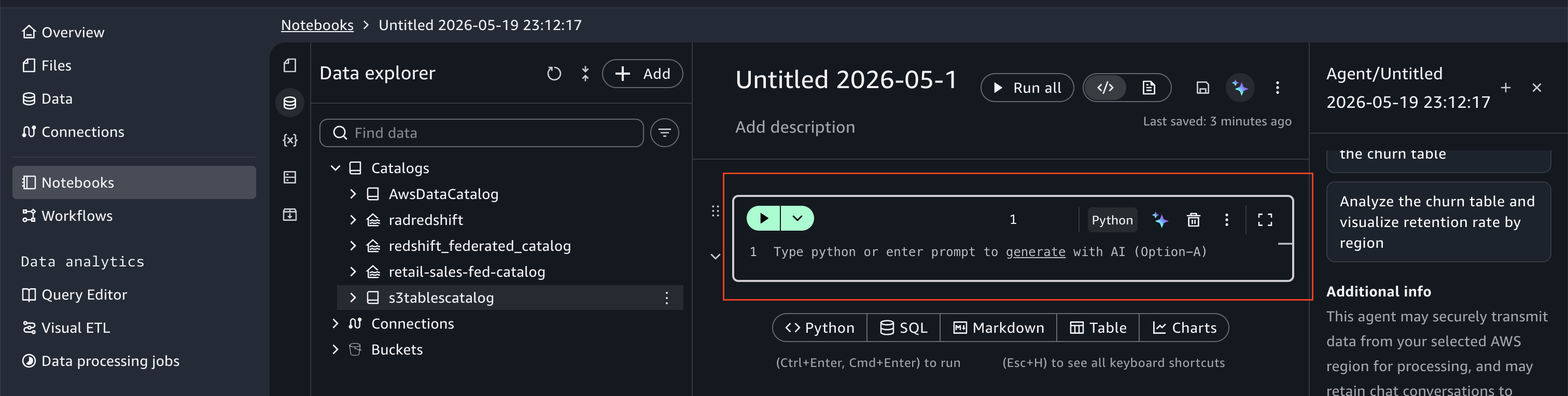
SageMaker Data Agent generating SQL from a natural language prompt

Figure 9: The SageMaker Data Agent generating SQL from a natural language request

Add each code block in a new cell by choosing the SQL button:
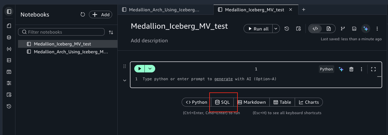
SQL cell-type button in the notebook toolbar

Figure 10: The SQL button for adding a code block to a notebook cell

Choose Athena Spark or Glue Spark as your compute from the cell menu.
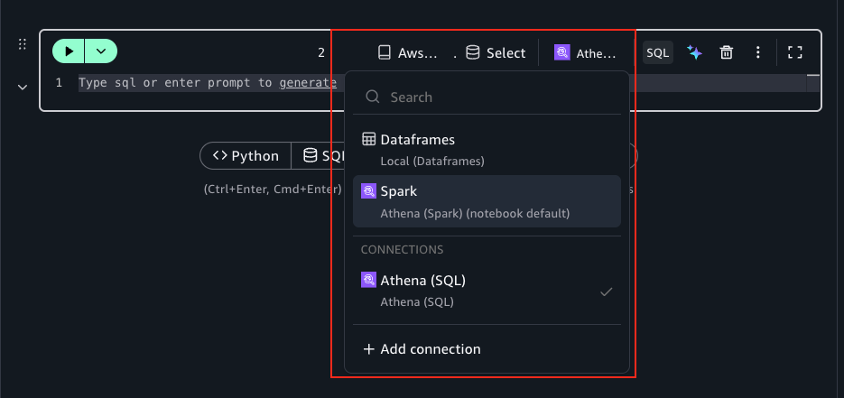
Compute connection selection in the notebook cell menu

Figure 11: The compute selection in the notebook cell menu

If you encounter errors after cell execution, use the data agent chatbot or the Fix with AI button to resolve them.
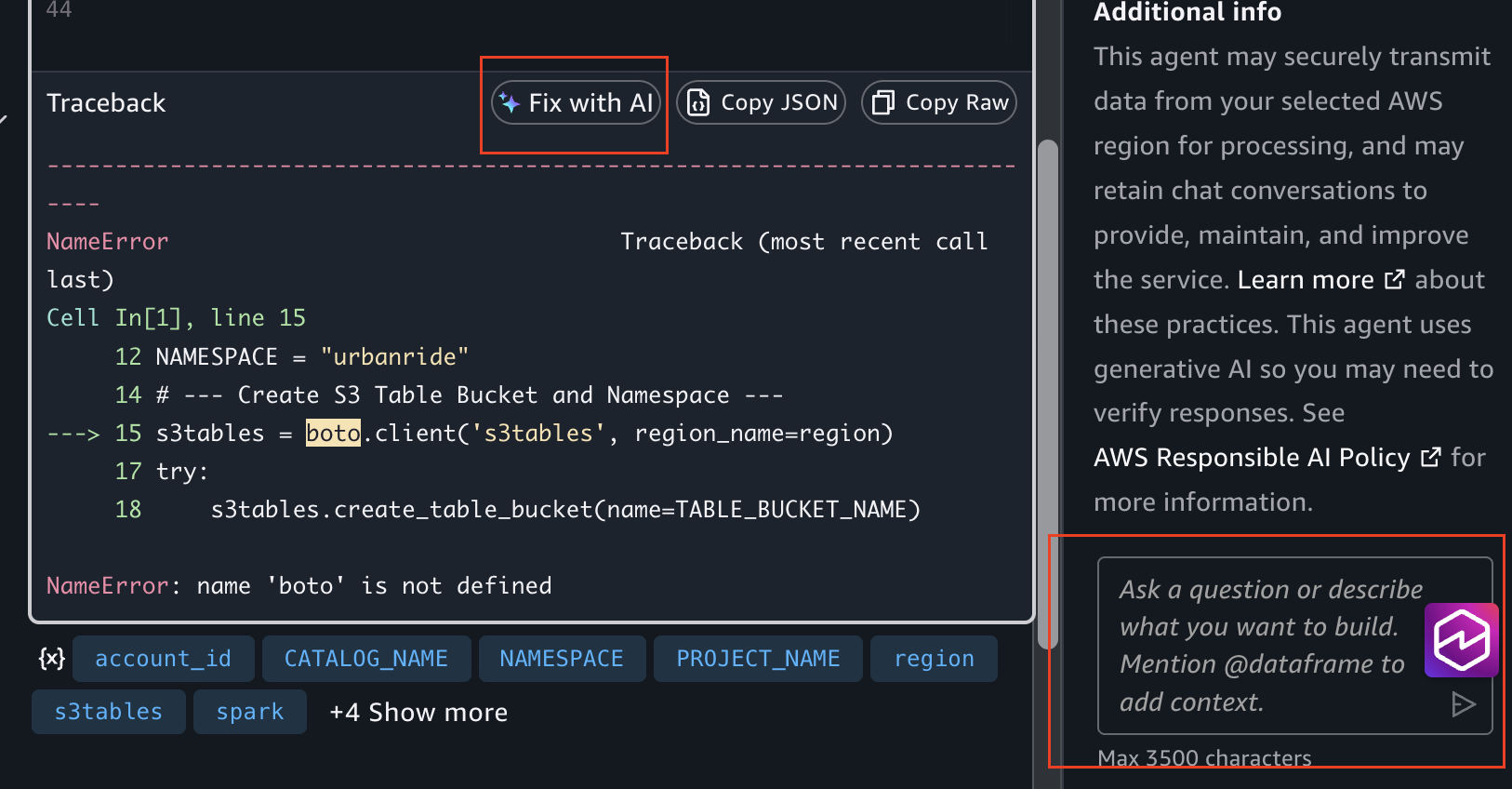
Fix with AI button and data agent chatbot for resolving cell errors

Figure 12: The Fix with AI button for resolving cell execution errors

Step 2: Ingest data into Bronze

Generate 300 realistic ride-sharing trips and insert them directly into the Bronze Iceberg table. This simulates a raw data ingestion layer. In production, you generally configure a streaming source or batch load based on your requirements.

Copy the following code into the first notebook cell (use a Python cell type).

import random
from datetime import datetime, timedelta

CITIES = {
    "San Francisco": {"lat_range": (37.70, 37.82), "lon_range": (-122.52, -122.38), "surge_prob": 0.3},
    "Austin": {"lat_range": (30.22, 30.40), "lon_range": (-97.80, -97.68), "surge_prob": 0.15},
    "Chicago": {"lat_range": (41.85, 41.95), "lon_range": (-87.70, -87.60), "surge_prob": 0.2},
    "Seattle": {"lat_range": (47.55, 47.68), "lon_range": (-122.40, -122.28), "surge_prob": 0.25},
}
VEHICLE_TYPES = ["UberX", "Comfort", "XL", "Black"]
PAYMENT_METHODS = ["credit_card", "debit_card", "apple_pay", "google_pay", "cash"]
STATUSES = ["completed"] * 4 + ["cancelled_rider", "cancelled_driver"]
BASE_FARES = {"UberX": 2.50, "Comfort": 3.50, "XL": 4.00, "Black": 7.00}
PER_MILE = {"UberX": 1.75, "Comfort": 2.25, "XL": 2.50, "Black": 3.75}
PER_MIN = {"UberX": 0.35, "Comfort": 0.45, "XL": 0.50, "Black": 0.65}

rows = []
for i in range(300):
    city_name = random.choice(list(CITIES.keys()))
    city = CITIES[city_name]
    vehicle = random.choice(VEHICLE_TYPES)
    duration = random.randint(5, 45)
    distance = round(random.uniform(1.0, 20.0), 1)
    surge = round(random.uniform(1.0, 2.5), 1) if random.random() < city["surge_prob"] else 1.0
    base = BASE_FARES[vehicle]
    fare = round((base + distance * PER_MILE[vehicle] + duration * PER_MIN[vehicle]) * surge, 2)
    tip = round(fare * random.choice([0, 0, 0.1, 0.15, 0.2, 0.25]), 2)
    status = random.choice(STATUSES)
    day = random.randint(0, 2)
    hour = random.choices(range(24),
        weights=[1,1,1,1,1,2,4,8,10,8,6,5,6,5,5,5,6,8,10,8,6,4,2,1])[0]
    trip_time = datetime(2025, 12, 1) + timedelta(days=day, hours=hour, minutes=random.randint(0, 59))

    rows.append((
        f"TRIP-{i+1:06d}",
        f"DRV-{random.randint(1000, 5000)}",
        f"RDR-{random.randint(10000, 99999)}",
        city_name, vehicle,
        round(random.uniform(*city["lat_range"]), 6),
        round(random.uniform(*city["lon_range"]), 6),
        round(random.uniform(*city["lat_range"]), 6),
        round(random.uniform(*city["lon_range"]), 6),
        trip_time.isoformat(),
        (trip_time + timedelta(minutes=duration)).isoformat(),
        duration, distance, surge, base, fare, tip, round(fare + tip, 2),
        random.choice(PAYMENT_METHODS),
        random.choice([None, 3, 4, 4, 5, 5, 5]) if status == "completed" else None,
        status,
    ))

schema = ("trip_id STRING, driver_id STRING, rider_id STRING, city STRING, "
    "vehicle_type STRING, pickup_lat DOUBLE, pickup_lon DOUBLE, "
    "dropoff_lat DOUBLE, dropoff_lon DOUBLE, trip_start_time STRING, "
    "trip_end_time STRING, duration_minutes INT, distance_miles DOUBLE, "
    "surge_multiplier DOUBLE, base_fare DOUBLE, trip_fare DOUBLE, "
    "tip_amount DOUBLE, total_amount DOUBLE, payment_method STRING, "
    "rating INT, status STRING")

df = spark.createDataFrame(rows, schema)
df.writeTo("{CATALOG_NAME}.{NAMESPACE_NAME}.trips_bronze").createOrReplace()

print(f"Created Table and Inserted {len(rows)} trips into Bronze layer")

Step 3: Explore Bronze

Run a preview on the bronze table. The output should look like the following screenshot:
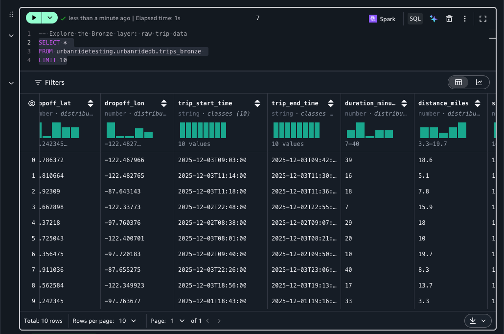
Preview of raw Bronze table trip records with string timestamps and nullable fields

Figure 13: A preview of raw trip records in the Bronze table

You should see raw, unprocessed trip records with string timestamps and nullable fields. This is exactly what the Silver layer will clean up.

Now, verify the ingested data by querying the Bronze table for basic statistics.

SELECT COUNT(*) as total_trips, COUNT(DISTINCT city) as cities,
COUNT(DISTINCT vehicle_type) as vehicle_types,
MIN(trip_start_time) as earliest, MAX(trip_start_time) as latest
FROM ({CATALOG_NAME}.{NAMESPACE_NAME}.trips_bronze

The output should look like the following screenshot:
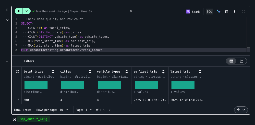
Query results showing total trips, distinct cities, and vehicle types in the Bronze table

Figure 14: Bronze table statistics showing total trips, distinct cities, and vehicle types

Step 4: Create the Silver materialized view

This SQL statement defines the Silver layer as a materialized view that cleans, transforms, and derives new columns from the Bronze table. Note that this is only a definition. The system processes the data at refresh time.

CREATE MATERIALIZED VIEW IF NOT EXISTS {CATALOG_NAME}.{DATABASE}.mv_trips_silver
COMMENT 'Silver layer: Cleaned trip data with proper types and derived columns'
SCHEDULE REFRESH EVERY 1 DAY
AS
SELECT
trip_id, driver_id, rider_id, city, vehicle_type,
pickup_lat, pickup_lon, dropoff_lat, dropoff_lon,
CAST(trip_start_time AS TIMESTAMP) as trip_start_timestamp,
CAST(trip_end_time AS TIMESTAMP) as trip_end_timestamp,
duration_minutes, distance_miles, surge_multiplier,
base_fare, trip_fare, tip_amount, total_amount,
payment_method, rating, status,
CASE WHEN distance_miles > 0 THEN total_amount / distance_miles ELSE 0 END as revenue_per_mile,
CASE WHEN rating >= 4 THEN 'High' WHEN rating >= 3 THEN 'Medium' ELSE 'Low' END as rating_category
FROM {CATALOG_NAME}.{DATABASE}.trips_bronze
WHERE trip_id IS NOT NULL AND driver_id IS NOT NULL AND rider_id IS NOT NULL
AND total_amount >= 0 AND distance_miles >= 0

print("Silver MV created: urbanride.mv_trips_silver")

Verify the Silver layer output:

SELECT trip_id, city, vehicle_type, total_amount,
ROUND(revenue_per_mile, 2) as rev_per_mile, rating_category
FROM {CATALOG_NAME}.{DATABASE}.mv_trips_silver LIMIT 5

Notice how the Silver layer now has proper timestamps, derived revenue_per_mile, and rating categories: clean, typed, and ready for you to aggregate.

The output should look like the following screenshot:
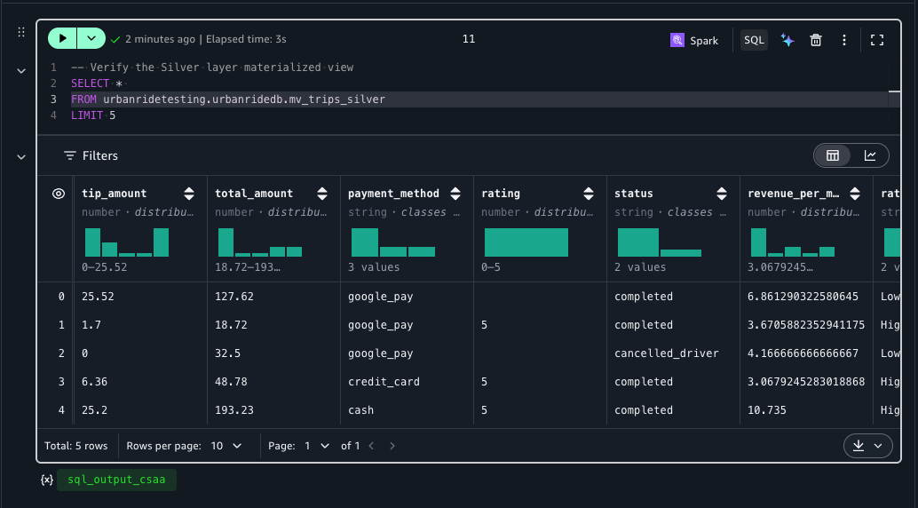
Silver materialized view results with typed timestamps, revenue_per_mile, and rating_category columns

Figure 15: Silver materialized view results with typed timestamps and derived columns

Step 5: Create Gold materialized views

Gold materialized views read incrementally from the Silver materialized view. This is a nested materialized view pattern: a materialized view built on top of another materialized view.

Gold 1: City daily metrics

With this materialized view, you can aggregate trip data by city and date with a scheduled daily refresh.

CREATE MATERIALIZED VIEW IF NOT EXISTS {CATALOG_NAME}.urbanride.mv_city_daily_metrics
COMMENT 'Gold layer: Daily aggregated metrics by city'
SCHEDULE REFRESH EVERY 1 DAY
AS
SELECT
city, DATE(trip_start_timestamp) as trip_date,
COUNT(*) as total_trips,
COUNT(DISTINCT driver_id) as active_drivers,
COUNT(DISTINCT rider_id) as active_riders,
SUM(total_amount) as total_revenue,
SUM(distance_miles) as total_distance,
SUM(tip_amount) as total_tips
FROM {CATALOG_NAME}.{DATABASE}.mv_trips_silver
WHERE status = 'completed'
GROUP BY city, DATE(trip_start_timestamp)

print("Gold MV created: mv_city_daily_metrics (reads from Silver MV, refreshes daily)")

Gold 2: Vehicle performance

With this materialized view, you can aggregate performance metrics by vehicle type and city.

CREATE MATERIALIZED VIEW IF NOT EXISTS {CATALOG_NAME}.{DATABASE}.mv_vehicle_performance
COMMENT 'Gold layer: Vehicle type performance metrics'
SCHEDULE REFRESH EVERY 1 DAY
AS
SELECT
vehicle_type, city,
COUNT(*) as trip_count,
SUM(total_amount) as total_revenue,
SUM(distance_miles) as total_distance,
SUM(tip_amount) as total_tips
FROM {CATALOG_NAME}.{DATABASE}.mv_trips_silver
WHERE status = 'completed'
GROUP BY vehicle_type, city

print("Gold MV created: mv_vehicle_performance (reads from Silver MV, refreshes daily)")

Dependency chain

The complete pipeline dependency is:

trips_bronze (table)
└── mv_trips_silver (materialized view)
    ├── mv_city_daily_metrics (MV on MV, daily schedule)
    └── mv_vehicle_performance (MV on MV, daily schedule)

Each layer is defined by a single SQL statement. There are no DAGs to maintain, no job definitions to deploy, and no watermark tracking to implement.

Step 6: Query the Gold layer

Query the Gold materialized views to see aggregated business metrics.

City daily metrics Gold table

SELECT city, trip_date, total_trips, active_drivers,
ROUND(total_revenue, 2) as revenue,
ROUND(total_revenue / total_trips, 2) as avg_per_trip
FROM {CATALOG_NAME}.{DATABASE}.mv_city_daily_metrics
ORDER BY trip_date DESC, revenue DESC LIMIT 15

The output should look like the following screenshot:
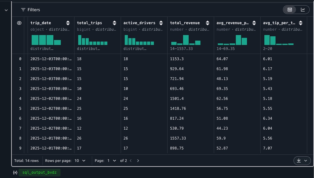
City daily metrics results with trips, active drivers, and revenue per city

Figure 16: City daily metrics from the Gold materialized view

Vehicle performance Gold table

SELECT vehicle_type, city, trip_count,
ROUND(total_revenue, 2) as revenue,
ROUND(total_revenue / trip_count, 2) as avg_per_trip
FROM {CATALOG_NAME}.{DATABASE}.mv_vehicle_performance
ORDER BY revenue DESC

The output should look like the following screenshot:
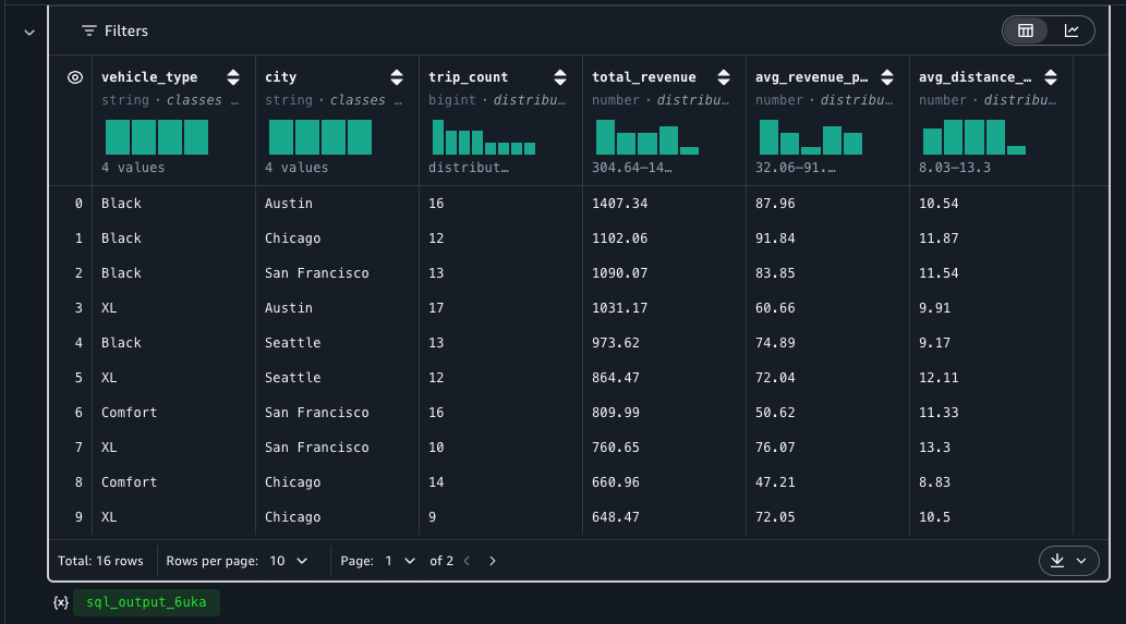
Vehicle performance results with trip counts and revenue by vehicle type and city

Figure 17: Vehicle performance metrics from the Gold materialized view

The Gold layer gives you pre-aggregated, business-ready metrics without writing aggregation jobs.

Step 7: Data propagation demo

This section demonstrates how changes propagate through the layers using INSERT, UPDATE (MERGE), and DELETE operations followed by incremental refresh. In production, the scheduled refresh handles this automatically. We trigger it manually here for demonstration purposes.

INSERT new records

Insert new trip records into the Bronze table.

INSERT INTO {CATALOG_NAME}.{DATABASE}.trips_bronze VALUES
('DEMO_TRIP_001', 'DRIVER_999', 'RIDER_888', 'Seattle', 'UberX',
47.6062, -122.3321, 47.6205, -122.3493,
'2024-12-15 14:30:00', '2024-12-15 14:50:00',
20, 5.2, 1.0, 10.0, 15.0, 3.0, 18.0, 'credit_card', 5, 'completed'),
('DEMO_TRIP_002', 'DRIVER_888', 'RIDER_777', 'Seattle', 'XL',
47.6101, -122.3300, 47.6550, -122.3080,
'2024-12-15 15:00:00', '2024-12-15 15:35:00',
35, 8.5, 1.5, 15.0, 30.0, 5.0, 35.0, 'cash', 4, 'completed'),
('DEMO_TRIP_003', 'DRIVER_777', 'RIDER_666', Portland, 'Comfort',
30.2672, -97.7431, 30.2800, -97.7400,
'2024-12-15 16:00:00', '2024-12-15 16:15:00',
15, 3.0, 1.0, 8.0, 12.0, 2.0, 14.0, 'credit_card', 5, 'completed')

print("Inserted 3 new trips into Bronze")

Refresh Silver (incremental)

Refresh the Silver materialized view. Iceberg materialized view processes only three new records.

REFRESH MATERIALIZED VIEW {CATALOG_NAME}.{DATABASE}.mv_trips_silver"

Verify the new records propagated

SELECT trip_id, city, total_amount, ROUND(revenue_per_mile, 2) as rev_per_mile, rating_category
FROM {CATALOG_NAME}.{DATABASE}.mv_trips_silver
WHERE trip_id LIKE 'DEMO_TRIP_%' ORDER BY trip_id

The output should look like the following screenshot:
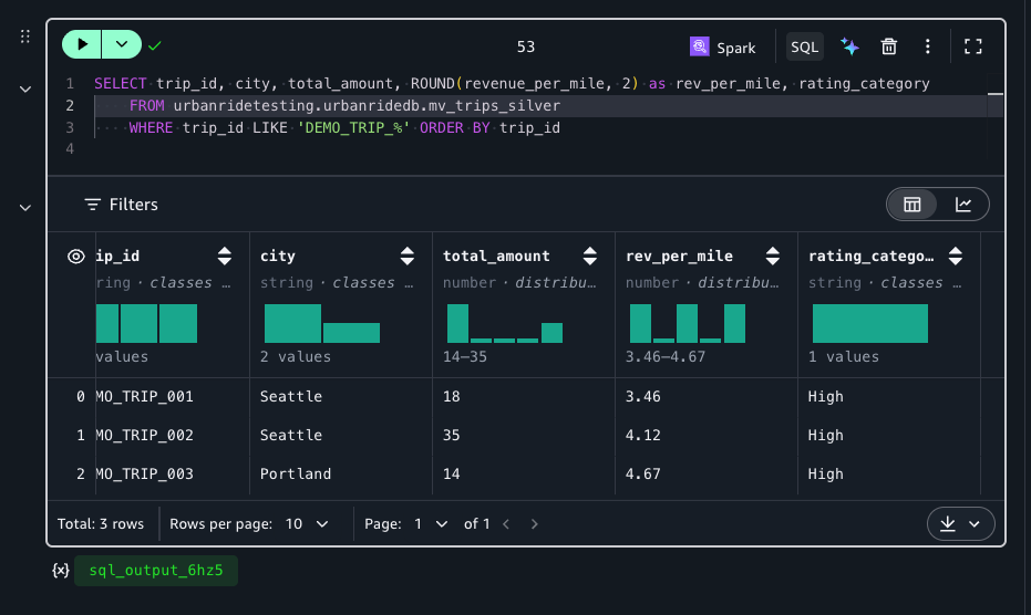
Silver materialized view showing three newly inserted demo trips

Figure 18: The Silver materialized view showing the three newly inserted demo trips

Refresh Gold (cascading from the Silver materialized view)

Refresh the Gold materialized view. It reads from the refreshed Silver materialized view and processes only the incremental changes.

REFRESH MATERIALIZED VIEW {CATALOG_NAME}.{DATABASE}.mv_city_daily_metrics

Verify the Gold layer reflects the new trips

SELECT city, trip_date, total_trips, ROUND(total_revenue, 2) as revenue
FROM {CATALOG_NAME}.{DATABASE}.mv_city_daily_metrics
WHERE trip_date = '2024-12-15' ORDER BY city

The output should look like the following screenshot:
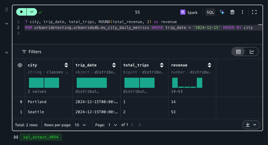
City daily metrics reflecting the newly added trips for December 15, 2024

Figure 19: City daily metrics reflecting the new trips for 2024-12-15

UPDATE through MERGE

Use MERGE to update existing records in Bronze, then refresh incrementally.

MERGE INTO {CATALOG_NAME}.{DATABASE}.trips_bronze AS target
USING (SELECT 'DEMO_TRIP_002' as trip_id, 5 as new_rating, 20.0 as new_tip) AS source
ON target.trip_id = source.trip_id
WHEN MATCHED THEN UPDATE SET
target.rating = source.new_rating,
target.tip_amount = source.new_tip,
target.total_amount = target.trip_fare + source.new_tip

Refresh Silver and verify

REFRESH MATERIALIZED VIEW {CATALOG_NAME}.{DATABASE}.mv_trips_silver")

SELECT trip_id, rating, rating_category, tip_amount, total_amount,
ROUND(revenue_per_mile, 2) as rev_per_mile
FROM {CATALOG_NAME}.{DATABASE}.mv_trips_silver WHERE trip_id = 'DEMO_TRIP_002'

print("UPDATE propagated: rating 4->5, tip $5->$20, total $35->$50")

The output should look like the following screenshot:
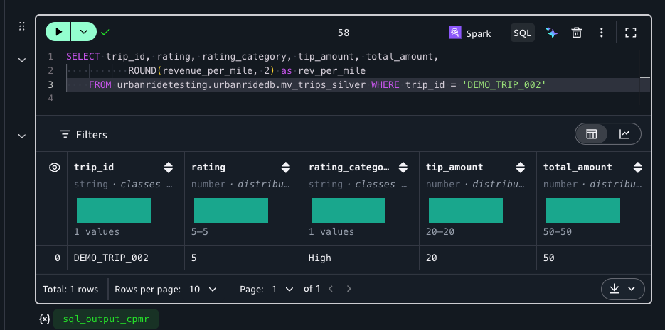
Silver materialized view showing the updated rating and tip for DEMO_TRIP_002

Figure 20: The Silver materialized view showing the updated rating and tip for the demo trip

Step 8: Cleanup

Drop materialized views, tables, the namespace, and delete the S3 Tables bucket to fully clean up resources.

# Drop MVs (Gold first, then Silver, due to dependency order)
spark.sql(f"DROP MATERIALIZED VIEW IF EXISTS {CATALOG_NAME}.{DATABASE}.mv_city_daily_metrics")
spark.sql(f"DROP MATERIALIZED VIEW IF EXISTS {CATALOG_NAME}.{DATABASE}.mv_vehicle_performance")
spark.sql(f"DROP MATERIALIZED VIEW IF EXISTS {CATALOG_NAME}.{DATABASE}.mv_trips_silver")
print("All materialized views dropped")

# Drop base table
spark.sql(f"DROP TABLE IF EXISTS {CATALOG_NAME}.{DATABASE}.trips_bronze")
print("Base table dropped")

# Drop the namespace
spark.sql(f"DROP NAMESPACE IF EXISTS {CATALOG_NAME}.{DATABASE} ")
print("Namespace dropped")

# Delete the S3 table bucket
import boto3
s3tables_client = boto3.client("s3tables")

# List and delete all remaining tables in the bucket
tables_response = s3tables_client.list_tables(
    tableBucketARN=TABLE_BUCKET_ARN, namespace="{DATABASE}"
)
for table in tables_response.get("tables", []):
    s3tables_client.delete_table(
        tableBucketARN=TABLE_BUCKET_ARN, namespace="{DATABASE}", name=table['name']
    )
    print(f" Deleted table: {table['name']}")

# Delete the namespace and bucket
s3tables_client.delete_namespace(tableBucketARN=TABLE_BUCKET_ARN, namespace="urbanride")
s3tables_client.delete_table_bucket(tableBucketARN=TABLE_BUCKET_ARN)
print(f"S3 table bucket deleted: {TABLE_BUCKET_NAME}")

Limitations and considerations

While materialized views remove most orchestration code, note the following:

  1. No sub-hour freshness. The minimum schedule granularity is one hour (SCHEDULE REFRESH EVERY 1 HOUR).
  2. Cascading refresh isn’t automatic. Refreshing Silver doesn’t trigger Gold in the same operation. Each layer refreshes on its own schedule or must be triggered sequentially.
  3. Deletes require a FULL refresh. An incremental REFRESH that feeds the Silver layer detects inserts and updates through Iceberg metadata but cannot detect row removals. Use REFRESH ... FULL when delete propagation is needed.
  4. SQL subset only. Some window functions, user-defined functions (UDFs), and complex expressions might not be supported in materialized view definitions.
  5. Schema evolution requires recreation. If the source schema changes in a way that affects the materialized view definition, you must drop and recreate it.
  6. AWS-specific extension. Iceberg materialized views are not part of the open-source Apache Iceberg specification. They aren’t portable to non-AWS environments.

Pricing

AWS bills materialized view auto-refresh at USD $0.44 per DPU-hour (4 vCPU, 16 GB memory), billed per second with a 1-minute minimum. When you configure scheduled refresh, the AWS Glue Data Catalog uses managed Spark compute to incrementally update the materialized view. You pay only for the compute time of each refresh run.

There are no separate charges for storing materialized view metadata in the Data Catalog (covered under standard catalog pricing: first million objects at no additional cost, then $1.00 per 100K objects/month). The materialized view data itself is stored as Iceberg files in S3 Tables or Amazon S3, charged at standard Amazon S3 storage rates.

Manual refreshes triggered from Spark (through Amazon Athena, Amazon EMR, or AWS Glue notebooks) are billed under those services’ respective compute pricing rather than the materialized view auto-refresh rate. For the latest pricing details, see the AWS Glue pricing page.

Estimated cost for this tutorial: Running through all steps once with 300 records typically consumes less than 0.5 DPU-hours total (~$0.22 in AWS Glue compute plus negligible Amazon S3 storage).

Summary

In this post, you built a Bronze → Silver → Gold medallion architecture using three SQL statements with nested materialized views and no orchestration code. The full pipeline creation took under 2 minutes, and incremental refreshes processed only changed data with no watermarks, no DAGs, no CDC plumbing.

To get started with your own data, create an Amazon SageMaker Unified Studio project, define your Bronze table, and express your transformation logic as Iceberg materialized views. For more information, see the Apache Iceberg materialized views documentation in the AWS Glue Developer Guide.

References

Using materialized views with AWS Glue

Query AWS Glue Data Catalog materialized views

Using materialized views with Amazon EMR

Working with Amazon S3 Tables and table buckets


About the authors

Gaurav Sharma

Gaurav Sharma

Gaurav is a Specialist Solutions Architect (Analytics) at AWS, supporting US public sector customers on their cloud journey. Outside of work, Gaurav enjoys spending time with his family and staying informed on technology, politics, and history through books, videos, and podcasts.

Matt David

Matt David

Matt is a Product Marketing Manager at AWS, specializing in helping data teams with AI-powered analytics. His areas of interest include self-service analytics, data democratization, and preparing organizations for the age of AI agents. He brings extensive experience from his roles at Atlassian, Hex, and DataCamp.

Define per-team resource limits for big data workloads using Amazon EMR Serverless

Post Syndicated from Gaurav Sharma original https://aws.amazon.com/blogs/big-data/define-per-team-resource-limits-for-big-data-workloads-using-amazon-emr-serverless/

Customers face a challenge when distributing cloud resources between different teams running workloads such as development, testing, or production. The resource distribution challenge also occurs when you have different line-of-business users. The objective is not only to ensure sufficient resources be consistently available to production workloads and critical teams, but also to prevent adhoc jobs from using all the resources and delaying other critical workloads due to mis-configured or non-optimized code. Cost controls and usage tracking across these teams is also a critical factor.

In the legacy big data and Hadoop clusters as well as Amazon EMR provisioned clusters, this problem was overcome by Yarn resource management and defining what were called Yarn queues for different workloads or teams. Another approach was to allocate independent clusters for different teams or different workloads.

Amazon EMR Serverless is a serverless option in Amazon EMR that makes it straightforward to run your big data workloads using open-source analytics frameworks such as Apache Spark and Hive without the need to configure, manage, or scale the clusters. With EMR Serverless, you don’t have to configure, optimize, secure, or operate clusters to run your workloads. You continue to get the benefits of Amazon EMR, such as open-source compatibility, concurrency, and optimized runtime performance for popular bigdata frameworks. EMR Serverless provides shorter job startup latency, automatic resource management and effective cost controls.

In this post, we show how to define per-team resource limits for big data workloads using EMR serverless.

Solution overview

EMR Serverless comes with a concept called an  EMR Serverless application, which is an isolated environment with the option to choose one of the open source analytics applications(Spark, Hive) to submit your workloads. You can include your own custom libraries, specify your EMR release version, and most importantly define the resource limits for the compute and memory resources. For instance, if your production Spark jobs run on Amazon EMR 6.9.0 and you need to test the same workload on Amazon EMR 6.10.0, you could use EMR Serverless to define EMR 6.10.0 as your version and test your workload using a predefined limit on resources.

The following diagram illustrates our solution architecture. We see that two different teams namely Prod team and Dev team are submitting their jobs independently to two different EMR Applications (namely ProdApp and DevApp respectively ) having dedicated resources.

EMR Serverless provides controls at the account, application and job level to limit the use of resources such as CPU, memory or disk. In the following sections, we discuss some of these controls.

Service quotas at account level

Amazon EMR Serverless has a default quota of 16 for maximum concurrent vCPUs per account. In other words, a new account can have a maximum of 16 vCPUs running at a given point in time in a particular Region across all EMR Serverless applications. However, this quota is auto-adjustable based on the usage patterns, which are monitored at the account and Region levels.

Resource limits and runtime configurations at the application level

In addition to quotas at the account levels, administrators can limit the use of resources at the application level using a feature known as “maximum capacity” which defines the maximum total vCPU, memory and disk capacity that can be consumed collectively by all the jobs running under this application.

You also have an option to specify common runtime and monitoring configurations at the application level which you would otherwise put in the specific job configurations. This helps create a standardized runtime environment for all the jobs running under an application. This can include settings like defining common connection setting your jobs need access to, log configurations that all your jobs will inherit by default, or Spark resource settings to help balance ad-hoc workloads. You can override these configurations at the job level, but defining them at the application can help reduce the configuration necessary for individual jobs.

For further details, refer to Declaring configurations at application level.

Runtime configurations at Job level

After you have set service, application quotas and runtime configurations at application level, you also have an option to override or add new configurations at the job level as well. For example, you can use different Spark job parameters to define how many maximum executors can be run by that specific job. One such parameter is spark.dynamicAllocation.maxExecutors which defines an upper bound for the number of executors in a job and therefore controls the number of workers in an EMR Serverless application because each executor runs within a single worker. This parameter is part of the dynamic allocation feature of Apache Spark, which allows you to dynamically scale the number of executors(workers) registered with the job up and down based on the workload. Dynamic allocation is enabled by default on EMR Serverless. For detailed steps, refer to Declaring configurations at application level.

With these configurations, you can control the resources used across accounts, applications, and jobs. For example, you can create applications with a predefined maximum capacity to constrain costs or configure jobs with resource limits in order to allow multiple ad hoc jobs to run simultaneously without consuming too many resources.

Best practices and considerations

Extending these usage scenarios further, EMR Serverless provides features and capabilities to implement the following design considerations and best practices based on your workload requirements:

  • To make sure that the users or teams submit their jobs only to their approved applications, you could use tag based AWS Identity and Access Management (IAM) policy conditions. For more details, refer to Using tags for access control.
  • You can use custom images as applications belonging to different teams that have distinct use-cases and software requirements. Using custom images is possible EMR 6.9.0 and onwards. Custom images allows you to package various application dependencies into a single container. Some of the important benefits of using custom images include the ability to use your own JDK and Python versions, apply your organization-specific security policies and integrate EMR Serverless into your build, test and deploy pipelines. For more information, refer to Customizing an EMR Serverless image.
  • If you need to estimate how much a Spark job would cost when run on EMR Serverless, you can use the open-source tool EMR Serverless Estimator. This tool analyzes Spark event logs to provide you with the cost estimate. For more details, refer to Amazon EMR Serverless cost estimator
  • We recommend that you determine your maximum capacity relative to the supported worker sizes by multiplying the number of workers by their size. For example, if you want to limit your application with 50 workers to 2 vCPUs, 16 GB of memory and 20 GB of disk, set the maximum capacity to 100 vCPU, 800 GB of memory, and 1000 GB of disk.
  • You can use tags when you create the EMR Serverless application to help search and filter your resources, or track the AWS costs using AWS Cost Explorer. You can also use tags for controlling who can submit jobs to a particular application or modify its configurations. Refer to Tagging your resources for more details.
  • You can configure the pre-initialized capacity at the time of application creation, which keeps the resources ready to be consumed by the time-sensitive jobs you submit.
  • The number of concurrent jobs you can run depends on important factors like maximum capacity limits, workers required for each job, and available IP address if using a VPC.
  • EMR Serverless will setup elastic network interfaces (ENIs) to securely communicate with resources in your VPC. Make sure you have enough IP addresses in your subnet for the job.
  • It’s a best practice to select multiple subnets from multiple Availability Zones. This is because the subnets you select determine the Availability Zones that are available to run the EMR Serverless application. Each worker uses an IP address in the subnet where it is launched. Make sure the configured subnets have enough IP addresses for the number of workers you plan to run.

Resource usage tracking

EMR Serverless not only allows cloud administrators to limit the resources for each application, it also enables them to monitor the applications and track the usage of resources across these applications. For more details, refer to  EMR Serverless usage metrics .

You can also deploy an AWS CloudFormation template to build a sample CloudWatch Dashboard for EMR Serverless which would help visualize various metrics for your applications and jobs. For more information, refer to EMR Serverless CloudWatch Dashboard.

Conclusion

In this post, we discussed how EMR Serverless empowers cloud and data platform administrators to efficiently distribute as well as restrict the cloud resources at different levels, for different organizational units, users and teams, as well as between critical and non-critical workloads. EMR Serverless resource limiting features make sure cloud cost is under control and resource usage is tracked effectively.

For more information on EMR Serverless applications and resource quotas, please refer to EMR Serverless User Guide and Configuring an application.


About the Authors

Gaurav Sharma is a Specialist Solutions Architect(Analytics) at Amazon Web Services (AWS), supporting US public sector customers on their cloud journey. Outside of work, Gaurav enjoys spending time with his family and reading books.

Damon Cortesi is a Principal Developer Advocate with Amazon Web Services. He builds tools and content to help make the lives of data engineers easier. When not hard at work, he still builds data pipelines and splits logs in his spare time.