All posts by Praveen Mohan Prasad

Reducing costs for shuffle-heavy Apache Spark workloads with serverless storage for Amazon EMR Serverless

Post Syndicated from Praveen Mohan Prasad original https://aws.amazon.com/blogs/big-data/reducing-costs-for-shuffle-heavy-apache-spark-workloads-with-serverless-storage-for-amazon-emr-serverless/

At re:Invent 2025, we announced serverless storage for Amazon EMR Serverless, eliminating the need to provision local disk storage for Apache Spark workloads. Serverless storage of Amazon EMR Serverless reduces data processing costs by up to 20% while helping prevent job failures from disk capacity constraints.

In this post, we explore the cost improvements we observed when benchmarking Apache Spark jobs with serverless storage on EMR Serverless. We take a deeper look at how serverless storage helps reduce costs for shuffle-heavy Spark workloads, and we outline practical guidance on identifying the types of queries that can benefit most from enabling serverless storage in your EMR Serverless Spark jobs.

Benchmark results for EMR 7.12 with serverless storage against standard disks

We conducted the performance and cost savings benchmarking using the TPC-DS dataset at 3TB scale, running 100+ queries that included a mix of high and low shuffle operations. The test configuration utilized Dynamic Resource Allocation (DRA) with no pre-initialized capacity. The system was set up with 20GB of disk space, and Spark configurations included 4 cores and 14GB memory for both driver and executor, with dynamic allocation starting at 3 initial executors (spark.dynamicAllocation.initialExecutors = 3). A comparative analysis was performed between local disk storage and serverless storage configurations. The aim was to assess both total and average cost implications between these storage approaches.

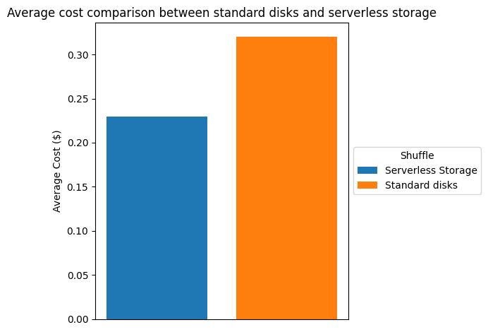
The following table and chart compare the cost reduction we observed in the testing environment described above. Based on us-east-1 pricing, we saw a cost savings of more than 26% when using serverless storage.

Shuffle
serverless storage standard Disks savings
Total Cost ($) 24.28 33.1 26.65%
Average Cost ($) 0.233 0.318 26.73%

Average cost comparison between standard disks and serverless storage

% Relative savings (per query) of serverless storage compared to standard disk shuffle

In this testing, we observed that serverless storage in EMR Serverless reduces cost for approximately 80% of TPC-DS queries. For the queries where it provides benefits, it delivers an average cost saving of approximately 47%, with savings of up to 85%. Queries that regress typically have low shuffle intensity, maintain high parallelism throughout execution, or complete quickly enough that executor scale-down opportunities are minimal. The following figure shows the percentage cost difference for each of the TPC-DS queries when serverless storage was enabled, compared to the baseline configuration without serverless storage. Positive values indicate cost savings (higher is better), while negative values indicate cost regressions.

Percentage cost savings per TPC-DS query with serverless storage enabled
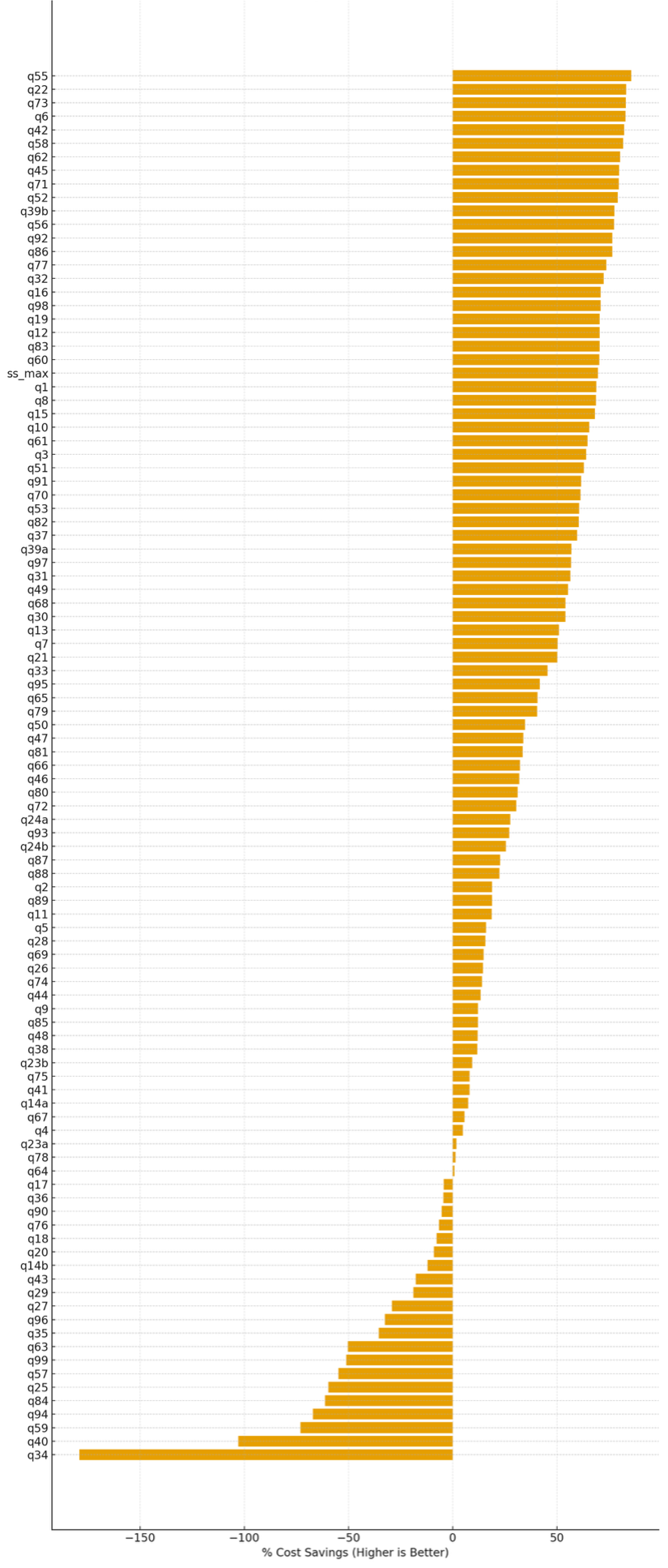
Percentage cost savings per TPC-DS query with serverless storage enabled

Runtime comparison

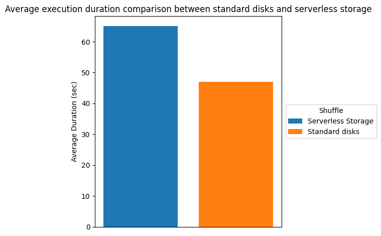
There is significant cost savings due to the increased elasticity from terminating executors earlier. However, job completion time may increase because the shuffle data is stored in serverless storage rather than locally on the executors. The additional read and write latency for shuffle data contributes to the longer runtime. The following table and chart show the runtime comparison, we observed in our testing environment.

Shuffle
serverless storage standard disks runtime
Total Duration (sec) 6770.63 4908.52 -37.94%
Average Duration (sec) 65.1 47.2 -37.92%

Runtime comparison

Storing shuffle externally and decoupling from the compute allowed the flexibility for EMR Serverless to turn off unused resources dynamically as the state info has been offloaded from the compute. However, these cost savings can be realized only when DRA is on. If DRA is turned off, Spark would keep those unused resources alive adding to the total cost.

Query patterns that benefit from serverless storage

The cost savings from serverless storage depend heavily on how executor demand changes across stages of a job. In this section, we examine common execution patterns and explain which query shapes are most likely to benefit from serverless storage of EMR Serverless and which query patterns may not benefit from shuffle externalization.

Inverted triangle pattern queries

In order to understand why externalizing the shuffle data can allow such a significant cost savings, consider a simplified query. The following query calculates annual total sales from the TPC-DS dataset by joining the store_sales and date_dim tables, summing the sales amounts per year, and ordering the results.

SELECT d_year, SUM(ss_net_paid) AS total_sales
FROM store_sales
JOIN date_dim ON store_sales.ss_sold_date_sk = date_dim.d_date_sk
GROUP BY d_year
ORDER BY d_year;

This query demonstrates that high executor demand during the map phase and low executor demand in the reduce phase is an aggregation query with a high cardinality input and a low cardinality group by.

  • Stage 1 (High Executor Demand)

The join and read steps scan the entire store_sales and date_dim tables. This often involves billions of rows in large-scale TPC-DS datasets, so Spark will try to parallelize the scan across many executors to maximize read throughput and compute efficiency.

  • Stage 2 (Low Executor Demand)

The aggregation is on d_year, which typically has few unique values, such as only a handful of years in the data. This means after the shuffle stage, the reduce phase combines the partial aggregates into a number of keys equal to the number of years (often < 10). Only a few Spark tasks are needed to finish the final aggregation, so most executors become idle.

With shuffle information stored on the local disk, the compute resources associated with these idle executors would still be running in order to keep the shuffle data available. With shuffle data offloaded from the nodes running the executors, with DRA enabled, those nodes with idle executors get released immediately.

Because early stages process high-cardinality inputs and later stages collapse data into a small number of keys, these queries form an “inverted triangle” execution pattern: wide parallelism at the top and narrow parallelism at the bottom as shown in the following image:
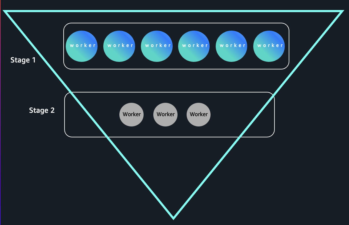
Inverted triangle pattern queries

Hourglass pattern queries

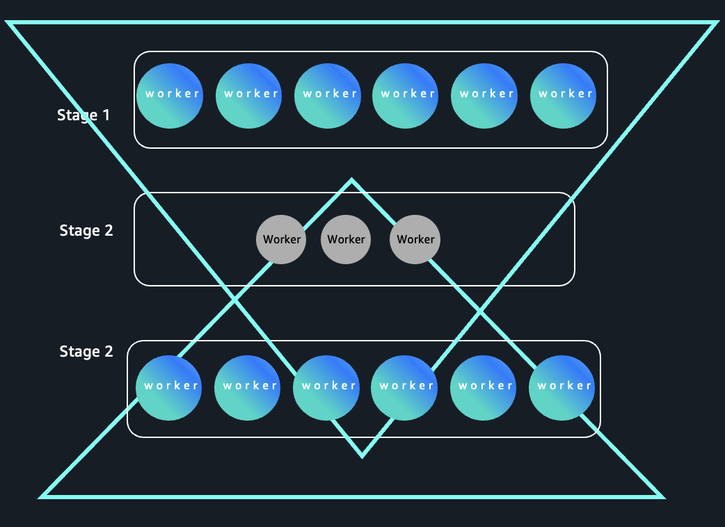
Depending upon the complexity of the job, there can be multiple stages with varying demand on number of executors needed for the stage. Such jobs can benefit from greater elasticity obtained by offloading shuffle data to external serverless storage. One such pattern is the hour glass pattern. The following figure shows a workload pattern where executor demand expands, contracts during shuffle-heavy stages, and expands again. Serverless storage of EMR Serverless decouples shuffle data from compute, enabling more efficient scale-down during narrow stages and helping improve cost optimization for elastic workloads.

 Hourglass pattern in Spark stage execution
Hourglass pattern queries

To identify queries of this category, consider the following example, The query progresses through three stages:

  • Stage 1: The initial join and filter between store_sales and item produces a wide, high-cardinality intermediate dataset, requiring high parallelism (many executors).
  • Stage 2: Aggregation groups by a small set of categories such as “Home” or “Electronics”, resulting in a drastic drop in output partitions. So this stage efficiently runs with only a few executors, as there’s little data to parallelize.
  • Stage 3: The small result is joined (usually a broadcast join) back to a large fact table with a date dimension, again producing a large result that is well-parallelized, causing Spark to ramp up executor usage for this stage.
WITH stage1_large_scan AS (
-- Stage 1: Scan and wide join generates lots of parallelism and needs many executors
SELECT ss_item_sk, ss_sold_date_sk, ss_net_paid, i_category
FROM store_sales
JOIN item ON store_sales.ss_item_sk = item.i_item_sk
WHERE item.i_category IN ('Home', 'Electronics')
),
stage2_small_agg AS (
-- Stage 2: Aggregate on low-cardinality column (by category), reducing to few groups, so few executors needed
SELECT i_category, SUM(ss_net_paid) AS total_cat_sales
FROM stage1_large_scan
GROUP BY i_category
),
stage3_broadcast_filter AS (
-- Stage 3: Join back to high-cardinality table, pushing parallelism up again
SELECT s.*, d.d_year
FROM store_sales s
JOIN date_dim d ON s.ss_sold_date_sk = d.d_date_sk
)

SELECT s3.d_year, s2.i_category, s2.total_cat_sales
FROM stage2_small_agg s2
JOIN stage3_broadcast_filter s3 ON s2.i_category = s3.i_category
ORDER BY s3.d_year, s2.i_category;

This pattern is common for reporting and dimensional analysis scenarios and is effective for demonstrating how Spark dynamically adjusts resource usage across job stages based on cardinality and parallelism needs. Such queries can also benefit from the elasticity enabled by external serverless storage.

Rectangle pattern queries

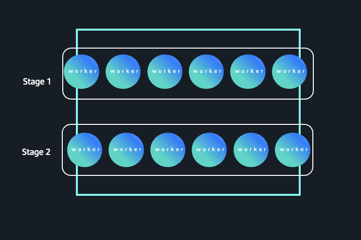
Not all queries benefit from externalizing the shuffle. Consider a query where the cardinality is high throughout, meaning both the stages operate on a large number of partitions and keys. Typically, queries that group by high-cardinality columns (such as item or customer) cause most stages to require similar amounts of parallelism. The following figure illustrates a Spark workload where parallelism remains consistently high across stages. In this pattern, both Stage 1 and Stage 2 operate on a large number of partitions and keys, resulting in sustained executor demand throughout the job lifecycle.

High-cardinality execution pattern with sustained parallelism
Rectangle pattern queries

The following query is the same query that we used in the inverted triangle pattern earlier, with one change. We have replaced the dim_date table (low cardinality) with item (high cardinality).

SELECT i_item_id, SUM(ss_net_paid) AS total_sales
FROM store_sales
JOIN item ON store_sales.ss_item_sk = item.i_item_sk
GROUP BY i_item_id
ORDER BY i_item_id
LIMIT 100;
  • Stage 1: Reads the rows from store_sales and joins with item, spreading data across many partitions—similar to the original query’s first stage.
  • Stage 2: The aggregation is by i_item_id, which normally has thousands to millions of distinct values in real datasets. This keeps parallelism high; many tasks handle non-overlapping keys, and shuffle outputs remain large.

There is no significant drop in cardinality: Because neither stage is reduced to a small group set, most executors stay busy throughout the job’s main phases, with little idle time even after the shuffle. This type of query results in a flatter executor utilization profile because each stage processes a similar volume of work, thus minimizing variation in resource utilization. These rectangle pattern queries will not see the cost benefit from the elasticity obtained by offloading shuffle data. However, there may still be other benefits such as reduction of job failures and performance bottlenecks from disk constraints, freedom from capacity planning and sizing, and provisioning of storage for intermediate data operations.

Conclusion

Serverless storage for Amazon EMR Serverless can deliver substantial cost savings for workloads with dynamic resource patterns, as seen in the 26% average cost savings we observed in our testing environment. By externalizing shuffle data, you can gain the elasticity to release idle executors immediately, demonstrated by the savings reaching up to 85% in our testing environment, on queries following inverted triangle and hourglass patterns when Dynamic Resource Allocation is enabled.Understanding your workload characteristics is key. While rectangle pattern queries may not see dramatic cost reductions, they can still benefit from improved reliability and removal of capacity planning overhead.

To get started: Analyze your job execution patterns, enable Dynamic Resource Allocation, and pilot serverless storage on shuffle-heavy workloads. Looking to reduce your Amazon EMR Serverless costs for Spark workloads? Explore serverless storage for EMR Serverless today.


About the authors

Sekar Srinivasan

Sekar Srinivasan

Sekar has over 20 years of experience working with data. He is passionate about helping customers build scalable solutions modernizing their architecture and generating insights from their data. In his spare time he likes to work on non-profit projects, especially those focused on underprivileged Children’s education.

Praveen Mohan Prasad

Praveen Mohan Prasad

Praveen is a data and AI Specialist with 10+ years of experience in distributed data systems and machine learning, specializing in Information Retrieval and vector search systems. Active open-source contributor and technical speaker in the ML-Search and Agentic-AI space.

Build multimodal search with Amazon OpenSearch Service

Post Syndicated from Praveen Mohan Prasad original https://aws.amazon.com/blogs/big-data/build-multimodal-search-with-amazon-opensearch-service/

Multimodal search enables both text and image search capabilities, transforming how users access data through search applications. Consider building an online fashion retail store: you can enhance the users’ search experience with a visually appealing application that customers can use to not only search using text but they can also upload an image depicting a desired style and use the uploaded image alongside the input text in order to find the most relevant items for each user. Multimodal search provides more flexibility in deciding how to find the most relevant information for your search.

To enable multimodal search across text, images, and combinations of the two, you generate embeddings for both text-based image metadata and the image itself. Text embeddings capture document semantics, while image embeddings capture visual attributes that help you build rich image search applications.

Amazon Titan Multimodal Embeddings G1 is a multimodal embedding model that generates embeddings to facilitate multimodal search. These embeddings are stored and managed efficiently using specialized vector stores such as Amazon OpenSearch Service, which is designed to store and retrieve large volumes of high-dimensional vectors alongside structured and unstructured data. By using this technology, you can build rich search applications that seamlessly integrate text and visual information.

Amazon OpenSearch Service and Amazon OpenSearch Serverless support the vector engine, which you can use to store and run vector searches. In addition, OpenSearch Service supports neural search, which provides out-of-the-box machine learning (ML) connectors. These ML connectors enable OpenSearch Service to seamlessly integrate with embedding models and large language models (LLMs) hosted on Amazon Bedrock, Amazon SageMaker, and other remote ML platforms such as OpenAI and Cohere. When you use the neural plugin’s connectors, you don’t need to build additional pipelines external to OpenSearch Service to interact with these models during indexing and searching.

This blog post provides a step-by-step guide for building a multimodal search solution using OpenSearch Service. You will use ML connectors to integrate OpenSearch Service with the Amazon Bedrock Titan Multimodal Embeddings model to infer embeddings for your multimodal documents and queries. This post illustrates the process by showing you how to ingest a retail dataset containing both product images and product descriptions into your OpenSearch Service domain and then perform a multimodal search by using vector embeddings generated by the Titan multimodal model. The code used in this tutorial is open source and available on GitHub for you to access and explore.

Multimodal search solution architecture

We will provide the steps required to set up multimodal search using OpenSearch Service. The following image depicts the solution architecture.

Multimodal search architecture

Figure 1: Multimodal search architecture

The workflow depicted in the preceding figure is:

  1. You download the retail dataset from Amazon Simple Storage Service (Amazon S3) and ingest it into an OpenSearch k-NN index using an OpenSearch ingest pipeline.
  2. OpenSearch Service calls the Amazon Bedrock Titan Multimodal Embeddings model to generate multimodal vector embeddings for both the product description and image.
  3. Through an OpenSearch Service client, you pass a search query.
  4. OpenSearch Service calls the Amazon Bedrock Titan Multimodal Embeddings model to generate vector embedding for the search query.
  5. OpenSearch runs the neural search and returns the search results to the client.

Let’s look at steps 1, 2, and 4 in more detail.

Step 1: Ingestion of the data into OpenSearch

This step involves the following OpenSearch Service features:

  • Ingest pipelines – An ingest pipeline is a sequence of processors that are applied to documents as they’re ingested into an index. Here you use a text_image_embedding processor to generate combined vector embeddings for the image and image description.
  • k-NN index – The k-NN index introduces a custom data type, knn_vector, which allows users to ingest vectors into an OpenSearch index and perform different kinds of k-NN searches. You use the k-NN index to store both the general field data types, such as text, numeric, etc., and specialized field data types, such as knn_vector.

Steps 2 and 4: OpenSearch calls the Amazon Bedrock Titan model

OpenSearch Service uses the Amazon Bedrock connector to generate embeddings for the data. When you send the image and text as part of your indexing and search requests, OpenSearch uses this connector to exchange the inputs with the equivalent embeddings from the Amazon Bedrock Titan model. The highlighted blue box in the architecture diagram depicts the integration of OpenSearch with Amazon Bedrock using this ML-connector feature. This direct integration eliminates the need for an additional component (for example, AWS Lambda) to facilitate the exchange between the two services.

Solution overview

In this post, you will build and run multimodal search using a sample retail dataset. You will use the same multimodal generated embeddings and experiment by running text search only, image search only and both text and image search in OpenSearch Service.

Prerequisites

  1. Create an OpenSearch Service domain. For instructions, see Creating and managing Amazon OpenSearch Service domains. Make sure the following settings are applied when you create the domain, while leaving other settings as default.
    • OpenSearch version is 2.13
    • The domain has public access
    • Fine-grained access control is enabled
    • A master user is created
  2. Set up a Python client to interact with the OpenSearch Service domain, preferably on a Jupyter Notebook interface.
  3. Add model access in Amazon Bedrock. For instructions, see add model access.

Note that you need to refer to the Jupyter Notebook in the GitHub repository to run the following steps using Python code in your client environment. The following sections provide the sample blocks of code that contain only the HTTP request path and the request payload to be passed to OpenSearch Service at every step.

Data overview and preparation

You will be using a retail dataset that contains 2,465 retail product samples that belong to different categories such as accessories, home decor, apparel, housewares, books, and instruments. Each product contains metadata including the ID, current stock, name, category, style, description, price, image URL, and gender affinity of the product. You will be using only the product image and product description fields in the solution.

A sample product image and product description from the dataset are shown in the following image:

Sample product image and description

Figure 2: Sample product image and description

In addition to the original product image, the textual description of the image provides additional metadata for the product, such as color, type, style, suitability, and so on. For more information about the dataset, visit the retail demo store on GitHub.

Step 1: Create the OpenSearch-Amazon Bedrock ML connector

The OpenSearch Service console provides a streamlined integration process that allows you to deploy an Amazon Bedrock-ML connector for multimodal search within minutes. OpenSearch Service console integrations provide AWS CloudFormation templates to automate the steps of Amazon Bedrock model deployment and Amazon Bedrock-ML connector creation in OpenSearch Service.

  1. In the OpenSearch Service console, navigate to Integrations as shown in the following image and search for Titan multi-modal. This returns the CloudFormation template named Integrate with Amazon Bedrock Titan Multi-modal, which you will use in the following steps.Configure domainFigure 3: Configure domain
  2. Select Configure domain and choose ‘Configure public domain’.
  3. You will be automatically redirected to a CloudFormation template stack as shown in the following image, where most of the configuration is pre-populated for you, including the Amazon Bedrock model, the ML model name, and the AWS Identity and Access Management (IAM) role that is used by Lambda to invoke your OpenSearch domain. Update Amazon OpenSearch Endpoint with your OpenSearch domain endpoint and Model Region with the AWS Region in which your model is available.Create a CloudFormation stackFigure 4: Create a CloudFormation stack
  4. Before you deploy the stack by clicking ‘Create Stack’, you need to give necessary permissions for the stack to create the ML connector. The CloudFormation template creates a Lambda IAM role for you with the default name LambdaInvokeOpenSearchMLCommonsRole, which you can override if you want to choose a different name. You need to map this IAM role as a Backend role for ml_full_access role in OpenSearch dashboards Security plugin, so that the Lambda function can successfully create the ML connector. To do so,
    • Login to the OpenSearch Dashboards using the master user credentials that you created as a part of prerequisites. You can find the Dashboards endpoint on your domain dashboard on the OpenSearch Service console.
    • From the main menu choose SecurityRoles, and select the ml_full_access role.
    • Choose Mapped usersManage mapping.
    • Under Backend roles, add the ARN of the Lambda role (arn:aws:iam::<account-id>:role/LambdaInvokeOpenSearchMLCommonsRole) that needs permission to call your domain.
    • Select Map and confirm the user or role shows up under Mapped users.Set permissions in OpenSearch dashboardsFigure 5: Set permissions in OpenSearch dashboards security plugin
  5. Return back to the CloudFormation stack console, check the box, ‘I acknowledge that AWS CloudFormation might create IAM resources with customised names‘ and click on ‘Create Stack’.
  6. After the stack is deployed, it will create the Amazon Bedrock-ML connector (ConnectorId) and a model identifier (ModelId). CloudFormation stack outputsFigure 6: CloudFormation stack outputs
  7. Copy the ModelId from the Outputs tab of the CloudFormation stack starting with prefix ‘OpenSearch-bedrock-mm-’ from your CloudFormation console. You will be using this ModelId in the further steps.

Step 2: Create the OpenSearch ingest pipeline with the text_image_embedding processor

You can create an ingest pipeline with the text_image_embedding processor, which transforms the images and descriptions into embeddings during the indexing process.

In the following request payload, you provide the following parameters to the text_image_embedding processor. Specify which index fields to convert to embeddings, which field should store the vector embeddings, and which ML model to use to perform the vector conversion.

  • model_id (<model_id>) – The model identifier from the previous step.
  • Embedding (<vector_embedding>) – The k-NN field that stores the vector embeddings.
  • field_map (<product_description> and <image_binary>) – The field name of the product description and the product image in binary format.
path = "_ingest/pipeline/<bedrock-multimodal-ingest-pipeline>"

..
payload = {
"description": "A text/image embedding pipeline",
"processors": [
{
"text_image_embedding": {
"model_id":<model_id>,
"embedding": <vector_embedding>,
"field_map": {
"text": <product_description>,
"image": <image_binary>
}}}]}

Step 4: Create the k-NN index and ingest the retail dataset

Create the k-NN index and set the pipeline created in the previous step as the default pipeline. Set index.knn to True to perform an approximate k-NN search. The vector_embedding field type must be mapped as a knn_vector. vector_embedding field dimension must be mapped with the number of dimensions of the vector that the model provides.

Amazon Titan Multimodal Embeddings G1 lets you choose the size of the output vector (either 256, 512, or 1024). In this post, you will be using the default 1024 dimensional vectors from the model. You can check the size of dimensions of the model by selecting ‘Providers’ -> ‘Amazon’ tab -> ‘Titan Multimodal Embeddings G1’ tab -> ‘Model attributes’, from your Bedrock console.

Given the smaller size of the dataset and to bias for better recall, you use the faiss engine with the hnsw algorithm and the default l2 space type for your k-NN index. For more information about different engines and space types, refer to k-NN index.

payload = {
"settings": {
"index.knn": True,
"default_pipeline": <ingest-pipeline>
},
"mappings": {
"properties": {
"vector_embedding": {
"type": "knn_vector",
"dimension": 1024
"method": {
"engine": "faiss",
"space_type": "l2",
"name": "hnsw",
"parameters": {}
}
},
"product_description": {"type": "text"},
"image_url": {"type": "text"},
"image_binary": {"type": "binary"}
}}}

Finally, you ingest the retail dataset into the k-NN index using a bulk request. For the ingestion code, refer to the step 7, ‘Ingest the dataset into k-NN index using Bulk request‘ in the Jupyter notebook.

Step 5: Perform multimodal search experiments

Perform the following experiments to explore multimodal search and compare results. For text search, use the sample query “Trendy footwear for women” and set the number of results to 5 (size) throughout the experiments.

Experiment 1: Lexical search

This experiment shows you the limitations of simple lexical search and how the results can be improved using multimodal search.

Run a match query against the product_description field by using the following example query payload:

payload = {
"query": {
"match": {
"product_description": {
"query": "Trendy footwear for women"
}
}
},
"size": 5
}

Results:

Lexical search results

Figure 7: Lexical search results

Observation:

As shown in the preceding figure, the first three results refer to a jacket, glasses, and scarf, which are irrelevant to the query. These were returned because of the matching keywords between the query, “Trendy footwear for women” and the product descriptions, such as “trendy” and “women.” Only the last two results are relevant to the query because they contain footwear items.

Only the last two products fulfil the intent of the query, which was to find products that match all words in the query.

Experiment 2: Multimodal search with only text as input

In this experiment, you will use the Titan Multimodal Embeddings model that you deployed previously and run a neural search with only “Trendy footwear for women” (text) as input.

In the k-NN vector field (vector_embedding) of the neural query, you pass the model_id, query_text, and k value as shown in the following example. k denotes the number of results returned by the k-NN search.

payload = {
"query": {
"neural": {
"vector_embedding": {
"query_text": "Trendy footwear for women",
"model_id": <model_id>,
"k": 5
}
}
},
"size": 5
}

Results:

Results from multimodal search using text

Figure 8: Results from multimodal search using text

Observation:

As shown in the preceding figure, all five results are relevant because each represents a style of footwear. Additionally, the gender preference from the query (women) is also matched in all the results, which indicates that the Titan multimodal embeddings preserved the gender context in both the query and nearest document vectors.

Experiment 3: Multimodal search with only an image as input

In this experiment, you will use only a product image as the input query.

You will use the same neural query and parameters as in the previous experiment but pass the query_image parameter instead of using the query_text parameter. You need to convert the image into binary format and pass the binary string to the query_image parameter:

Image of a woman’s sandal used as the query input

Figure 9: Image of a woman’s sandal used as the query input

payload = {
"query": {
"neural": {
"vector_embedding": {
"query_image": <query_image_binary>,
"model_id": <model_id>,
"k": 5
}
}
},
"size": 5
}

Results:

Results from multimodal search using an image

Figure 10: Results from multimodal search using an image

Observation:

As shown in the preceding figure, by passing an image of a woman’s sandal, you were able to retrieve similar footwear styles. Though this experiment provides a different set of results compared to the previous experiment, all the results are highly related to the search query. All the matching documents are similar to the searched product image, not only in terms of the product category (footwear) but also in terms of the style (summer footwear), color, and gender affinity of the product.

Experiment 4: Multimodal search with both text and an image

In this last experiment, you will run the same neural query but pass both the image of a woman’s sandal and the text, “dark color” as inputs.

Figure 11: Image of a woman’s sandal used as part of the query input

As before, you will convert the image into its binary form before passing it to the query:

payload = {
"query": {
"neural": {
"vector_embedding": {
"query_image": <query_image_binary>,
"query_text": "dark color",
"model_id": <model_id>,
"k": 5
}
}
},
"size": 5
}

Results:

payload = { "query": { "neural": { "vector_embedding": { "query_image": <query_image_binary>, "query_text": "dark color", "model_id": <model_id>, "k": 5 } } }, "size": 5 }” width=”904″ height=”796″></a></p>
<p><em>Figure 12: Results of query using text and an image</em></p>
<h4><strong>Observation:</strong></h4>
<p>In this experiment, you augmented the image query with a text query to return dark, summer-style shoes. This experiment provided more comprehensive options by taking into consideration both text and image input.</p>
<h2>Overall observations</h2>
<p>Based on the experiments, all the variants of multimodal search provided more relevant results than a basic lexical search. After experimenting with text-only search, image-only search, and a combination of the two, it’s clear that the combination of text and image modalities provides more search flexibility and, as a result, more specific footwear options to the user.</p>
<h2>Clean up</h2>
<p>To avoid incurring continued AWS usage charges, delete the Amazon OpenSearch Service domain that you created and delete the CloudFormation stack starting with prefix ‘<strong>OpenSearch-bedrock-mm-</strong>’ that you deployed to create the ML connector.</p>
<h2>Conclusion</h2>
<p>In this post, we showed you how to use OpenSearch Service and the Amazon Bedrock Titan Multimodal Embeddings model to run multimodal search using both text and images as inputs. We also explained how the new multimodal processor in OpenSearch Service makes it easier for you to generate text and image embeddings using an OpenSearch ML connector, store the embeddings in a k-NN index, and perform multimodal search.</p>
<p>Learn more about <a href=ML-powered search with OpenSearch and set up you multimodal search solution in your own environment using the guidelines in this post. The solution code is also available on the GitHub repo.


About the Authors

Praveen Mohan Prasad is an Analytics Specialist Technical Account Manager at Amazon Web Services and helps customers with pro-active operational reviews on analytics workloads. Praveen actively researches on applying machine learning to improve search relevance.

Hajer Bouafif is an Analytics Specialist Solutions Architect at Amazon Web Services. She focuses on Amazon OpenSearch Service and helps customers design and build well-architected analytics workloads in diverse industries. Hajer enjoys spending time outdoors and discovering new cultures.

Aruna Govindaraju is an Amazon OpenSearch Specialist Solutions Architect and has worked with many commercial and open-source search engines. She is passionate about search, relevancy, and user experience. Her expertise with correlating end-user signals with search engine behavior has helped many customers improve their search experience. Her favourite pastime is hiking the New England trails and mountains.