Post Syndicated from Saunak Chandra original https://aws.amazon.com/blogs/big-data/using-the-amazon-redshift-data-api-to-interact-from-an-amazon-sagemaker-jupyter-notebook/
The Amazon Redshift Data API makes it easy for any application written in Python, Go, Java, Node.JS, PHP, Ruby, and C++ to interact with Amazon Redshift. Traditionally, these applications use JDBC connectors to connect, send a query to run, and retrieve results from the Amazon Redshift cluster. This requires extra steps like managing the cluster credentials and configuring the VPC subnet and security group.
In some use cases, you don’t want to manage connections or pass credentials on the wire. The Data API simplifies these steps so you can focus on data consumption instead of managing resources such as the cluster credentials, VPCs, and security groups.
This post demonstrates how you can connect an Amazon SageMaker Jupyter notebook to the Amazon Redshift cluster and run Data API commands in Python. The in-place analysis is an effective way to pull data directly into a Jupyter notebook object. We provide sample code to demonstrate in-place analysis by fetching Data API results into a Pandas DataFrame for quick analysis. For more information about the Data API, see Using the Amazon Redshift Data API to interact with Amazon Redshift clusters.
After exploring the mechanics of the Data API in a Jupyter notebook, we demonstrate how to implement a machine learning (ML) model in Amazon SageMaker, using data stored in the Amazon Redshift cluster. We use sample data to build, train, and test an ML algorithm in Amazon SageMaker. Finally, we deploy the model in an Amazon SageMaker instance and draw inference.
Using the Data API in a Jupyter notebook
Jupyter Notebook is a popular data exploration tool primarily used for ML. To work with ML-based analysis, data scientists pull data from sources like websites, Amazon Simple Storage Service (Amazon S3), and databases using Jupyter notebooks. Many Jupyter Notebook users prefer to use data from Amazon Redshift as their primary source of truth for their organization’s data warehouse and event data stored in Amazon S3 data lake.
When you use Amazon Redshift as a data source in Jupyter Notebook, the aggregated data is visualized first for preliminary analysis, followed by extensive ML model building, training, and deployment. Jupyter Notebook connects and runs SQL queries on Amazon Redshift using a Python-based JDBC driver. Data extraction via JDBC drivers poses the following challenges:
- Dealing with driver installations, credentials and network security management, connection pooling, and caching the result set
- Additional administrative overhead to bundle the drivers into the Jupyter notebook before sharing the notebook with others
The Data API simplifies these management steps. Jupyter Notebook is pre-loaded with libraries needed to access the Data API, which you import when you use data from Amazon Redshift.
Prerequisites
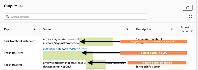
To provision the resources for this post, you launch the following AWS CloudFormation stack:

The CloudFormation template is tested in the us-east-2 Region. It launches a 2-node DC2.large Amazon Redshift cluster to work on for this post. It also launches an AWS Secrets Manager secret and an Amazon SageMaker Jupyter notebook instance.
The following screenshot shows the Outputs tab for the stack on the AWS CloudFormation console.

The Secrets Manager secret is updated with cluster details required to work with the Data API. An AWS Lambda function is spun up and run during the launch of the CloudFormation template to update the secret (it receives input from the launched Amazon Redshift cluster). The following code updates the secret:
SecretsUpdateFunction:
    Type: AWS::Lambda::Function
    Properties:
      Role: !GetAtt 'LambdaExecutionRole.Arn'
      FunctionName: !Join ['-', ['update_secret', !Ref 'AWS::StackName']]
      MemorySize: 2048
      Runtime: python3.7
      Timeout: 900
      Handler: index.handler
      Code:
        ZipFile:
          Fn::Sub:
          - |-
           import json
           import boto3
           import os
           import logging
           import cfnresponse

           LOGGER = logging.getLogger()
           LOGGER.setLevel(logging.INFO)

           ROLE_ARN = '${Role}'
           SECRET = '${Secret}'
           CLUSTER_ID = CLUSTER_ENDPOINT.split('.')[0]
           DBNAME = 'nyctaxi'

           def handler(event, context):

               # Get CloudFormation-specific parameters, if they exist
               cfn_stack_id = event.get('StackId')
               cfn_request_type = event.get('RequestType')

               #update Secrets Manager secret with host and port
               sm = boto3.client('secretsmanager')
               sec = json.loads(sm.get_secret_value(SecretId=SECRET)['SecretString'])
               sec['dbClusterIdentifier'] = CLUSTER_ID
               sec['db'] = DBNAME
               newsec = json.dumps(sec)
               response = sm.update_secret(SecretId=SECRET, SecretString=newsec)


               # Send a response to CloudFormation pre-signed URL
               cfnresponse.send(event, context, cfnresponse.SUCCESS, {
                   'Message': 'Secrets upated'
                   },
                   context.log_stream_name)

               return {
                   'statusCode': 200,
                   'body': json.dumps('Secrets updated')
               }

          - {
            Role : !GetAtt RedshiftSagemakerRole.Arn,
            Endpoint: !GetAtt RedshiftCluster.Endpoint.Address,
            Secret: !Ref RedshiftSecret
            }
Working with the Data API in Jupyter Notebook
In this section, we walk through the details of working with the Data API in a Jupyter notebook.
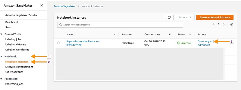
- On the Amazon SageMaker console, under Notebook, choose Notebook instances.
- Locate the notebook you created with the CloudFormation template.
- Choose Open Jupyter.

This opens up an empty Amazon SageMaker notebook page.
- Download the file RedshiftDeepAR-DataAPI.ipynb to your local storage.
- Choose Upload.
- Upload
RedshiftDeepAR-DataAPI.ipynb.
Importing Python packages
We first import the necessary boto3 package. A few other packages are also relevant for the analysis, which we import in the first cell. See the following code:
import botocore.session as s
from botocore.exceptions import ClientError
import boto3.session
import json
import boto3
import sagemaker
import operator
from botocore.exceptions import WaiterError
from botocore.waiter import WaiterModel
from botocore.waiter import create_waiter_with_client

import s3fs
import time
import os
import random
import datetime

import pandas as pd
import numpy as np
import matplotlib.pyplot as plt

from ipywidgets import interact, interactive, fixed, interact_manual
import ipywidgets as widgets
from ipywidgets import IntSlider, FloatSlider, Checkbox
Custom waiter
The Data API calls an HTTPS endpoint. Because ExecuteStatement Data API calls are asynchronous, we need a custom waiter. See the following code:
# Create custom waiter for the Redshift Data API to wait for finish execution of current SQL statement
waiter_name = 'DataAPIExecution'
JSON
delay=2
max_attempts=3

#Configure the waiter settings
waiter_config = {
  'version': 2,
  'waiters': {
    'DataAPIExecution': {
      'operation': 'DescribeStatement',
      'delay': delay,
      'maxAttempts': max_attempts,
      'acceptors': [
        {
          "matcher": "path",
          "expected": "FINISHED",
          "argument": "Status",
          "state": "success"
        },
        {
          "matcher": "pathAny",
          "expected": ["PICKED","STARTED","SUBMITTED"],
          "argument": "Status",
          "state": "retry"
        },
        {
          "matcher": "pathAny",
          "expected": ["FAILED","ABORTED"],
          "argument": "Status",
          "state": "failure"
        }
      ],
    },
  },
}
Retrieving information from Secrets Manager
We need to retrieve the following information from Secrets Manager for the Data API to use:
- Cluster identifier
- Secrets ARN
- Database name
Retrieve the above information using the following code:
secret_name='redshift-dataapidemo' ## replace the secret name with yours
session = boto3.session.Session()
region = session.region_name

client = session.client(
        service_name='secretsmanager',
        region_name=region
    )

try:
    get_secret_value_response = client.get_secret_value(
            SecretId=secret_name
        )
    secret_arn=get_secret_value_response['ARN']

except ClientError as e:
    print("Error retrieving secret. Error: " + e.response['Error']['Message'])

else:
    # Depending on whether the secret is a string or binary, one of these fields will be populated.
    if 'SecretString' in get_secret_value_response:
        secret = get_secret_value_response['SecretString']
    else:
        secret = base64.b64decode(get_secret_value_response['SecretBinary'])

secret_json = json.loads(secret)

cluster_id=secret_json['dbClusterIdentifier']
db=secret_json['db']
print("Cluster_id: " + cluster_id + "\nDB: " + db + "\nSecret ARN: " + secret_arn)
We now create the Data API client. For the rest of the notebook, we use the Data API client client_redshift. See the following code:
bc_session = s.get_session()

session = boto3.Session(
        botocore_session=bc_session,
        region_name=region,
    )

# Setup the client
client_redshift = session.client("redshift-data")
print("Data API client successfully loaded")
Listing the schema and tables
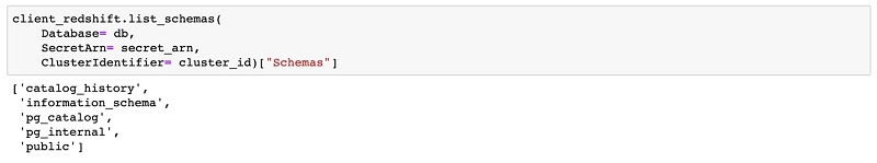
To list the schema, enter the following code:
client_redshift.list_schemas(
    Database= db,
    SecretArn= secret_arn,
    ClusterIdentifier= cluster_id)["Schemas"]
The following screenshot shows the output.

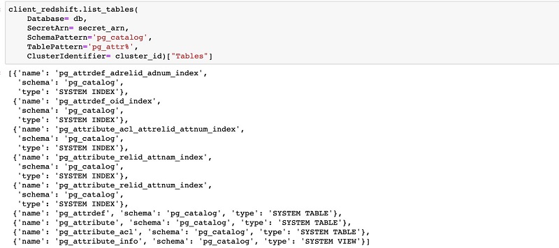
To list the tables, enter the following code:
client_redshift.list_schemas(
    Database= db,
    SecretArn= secret_arn,
    ClusterIdentifier= cluster_id)["Schemas"]
The following screenshot shows the output.

Creating the schema and table
Before you issue any SQL statement to the Data API, we instantiate the custom waiter. See the following code:
waiter_model = WaiterModel(waiter_config)
custom_waiter = create_waiter_with_client(waiter_name, waiter_model, client_redshift)

query_str = "create schema taxischema;"

res = client_redshift.execute_statement(Database= db, SecretArn= secret_arn, Sql= query_str, ClusterIdentifier= cluster_id)
id=res["Id"]

# Waiter in try block and wait for DATA API to return
try:
    custom_waiter.wait(Id=id)
except WaiterError as e:
    print (e)

desc=client_redshift.describe_statement(Id=id)
print("Status: " + desc["Status"] + ". Excution time: %d miliseconds" %float(desc["Duration"]/pow(10,6)))

query_str = 'create table taxischema.nyc_greentaxi(\
vendorid varchar(10),\
lpep_pickup_datetime timestamp,\
lpep_dropoff_datetime timestamp,\
store_and_fwd_flag char(1),\
ratecodeid int,\
pulocationid int,\
dolocationid int,\
passenger_count int,\
trip_distance decimal(8,2),\
fare_amount decimal(8,2),\
extra decimal(8,2),\
mta_tax decimal(8,2),\
tip_amount decimal(8,2),\
tolls_amount decimal(8,2),\
ehail_fee varchar(100),\
improvement_surcharge decimal(8,2),\
total_amount decimal(8,2),\
payment_type varchar(10),\
trip_type varchar(10),\
congestion_surcharge decimal(8,2)\
)\
sortkey (vendorid);'

res = client_redshift.execute_statement(Database= db, SecretArn= secret_arn, Sql= query_str, ClusterIdentifier= cluster_id)
id=res["Id"]

try:
    custom_waiter.wait(Id=id)
    print("Done waiting to finish Data API.")
except WaiterError as e:
    print (e)

desc=client_redshift.describe_statement(Id=id)
print("Status: " + desc["Status"] + ". Excution time: %d miliseconds" %float(desc["Duration"]/pow(10,6)))
Loading data into the cluster
After we create the table, we’re ready to load some data into it. The following code loads Green taxi cab data from two different Amazon S3 locations using individual COPY statements that run in parallel:
redshift_iam_role = sagemaker.get_execution_role()
print("IAM Role: " + redshift_iam_role)
source_s3_region='us-east-1'

# Reset the 'delay' attribute of the waiter to 30 seconds for long running COPY statement.
waiter_config["waiters"]["DataAPIExecution"]["delay"] = 20
waiter_model = WaiterModel(waiter_long_config)
custom_waiter = create_waiter_with_client(waiter_name, waiter_model, client_redshift)

query_copystr1 = "COPY taxischema.nyc_greentaxi FROM 's3://nyc-tlc/trip data/green_tripdata_2020' IAM_ROLE '" + redshift_iam_role + "' csv ignoreheader 1 region '" + source_s3_region + "';"

query_copystr2 = "COPY taxischema.nyc_greentaxi FROM 's3://nyc-tlc/trip data/green_tripdata_2019' IAM_ROLE '" + redshift_iam_role + "' csv ignoreheader 1 region '" + source_s3_region + "';"

## Execute 2 COPY statements in paralell
res1 = client_redshift.execute_statement(Database= db, SecretArn= secret_arn, Sql= query_copystr1, ClusterIdentifier= cluster_id)
res2 = client_redshift.execute_statement(Database= db, SecretArn= secret_arn, Sql= query_copystr2, ClusterIdentifier= cluster_id)

print("Redshift COPY started ...")

id1 = res1["Id"]
id2 = res2["Id"]
print("\nID: " + id1)
print("\nID: " + id2)

# Waiter in try block and wait for DATA API to return
try:
    custom_waiter.wait(Id=id1)
    print("Done waiting to finish Data API for the 1st COPY statement.")
    custom_waiter.wait(Id=id2)
    print("Done waiting to finish Data API for the 2nd COPY statement.")
except WaiterError as e:
    print (e)

desc=client_redshift.describe_statement(Id=id1)
print("[1st COPY] Status: " + desc["Status"] + ". Excution time: %d miliseconds" %float(desc["Duration"]/pow(10,6)))
desc=client_redshift.describe_statement(Id=id2)
print("[2nd COPY] Status: " + desc["Status"] + ". Excution time: %d miliseconds" %float(desc["Duration"]/pow(10,6)))
Performing in-place analysis
We can run the Data API to fetch the query result into a Pandas DataFrame. This simplifies the in-place analysis of the Amazon Redshift cluster data because we bypass unloading the data first into Amazon S3 and then loading it into a Pandas DataFrame.
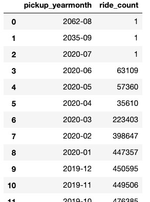
The following query lists records loaded in the table nyc_greentaxi by year and month:
query_str = "select to_char(lpep_pickup_datetime, 'YYYY-MM') as Pickup_YearMonth, count(*) as Ride_Count from taxischema.nyc_greentaxi group by 1 order by 1 desc;"

res = client_redshift.execute_statement(Database= db, SecretArn= secret_arn, Sql= query_str, ClusterIdentifier= cluster_id)

id = res["Id"]
# Waiter in try block and wait for DATA API to return
try:
    custom_waiter.wait(Id=id)
    print("Done waiting to finish Data API.")
except WaiterError as e:
    print (e)

output=client_redshift.get_statement_result(Id=id)
nrows=output["TotalNumRows"]
ncols=len(output["ColumnMetadata"])
#print("Number of columns: %d" %ncols)
resultrows=output["Records"]

col_labels=[]
for i in range(ncols): col_labels.append(output["ColumnMetadata"][i]['label'])

records=[]
for i in range(nrows): records.append(resultrows[i])

df = pd.DataFrame(np.array(resultrows), columns=col_labels)

df[col_labels[0]]=df[col_labels[0]].apply(operator.itemgetter('stringValue'))
df[col_labels[1]]=df[col_labels[1]].apply(operator.itemgetter('longValue'))

df
The following screenshot shows the output.

Now that you’re familiar with the Data API in Jupyter Notebook, let’s proceed with ML model building, training, and deployment in Amazon SageMaker.
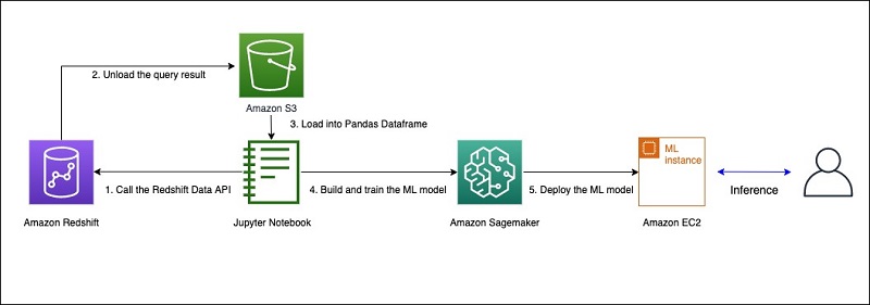
ML models with Amazon Redshift
The following diagram shows the ML model building, training, and deployment process. The source of data for ML training and testing is Amazon Redshift.

The workflow includes the following steps:
- Launch a Jupyter notebook instance in Amazon SageMaker. You make the Data API call from the notebook instance that runs a query in Amazon Redshift.
- The query result is unloaded into an S3 bucket. The output data is formatted as CSV, GZIP, or Parquet.
- Read the query result from Amazon S3 into a Pandas DataFrame within the Jupyter notebook. This DataFrame is split between train and test data accordingly.
- Build the model using the DataFrame, then train and test the model.
- Deploy the model into a dedicated instance in Amazon SageMaker. End-users and other systems can call this instance to directly infer by providing the input data.
Building and training the ML model using data from Amazon Redshift
In this section, we review the steps to build and train an Amazon SageMaker model from data in Amazon Redshift. For this post, we use the Amazon SageMaker built-in forecasting algorithm DeepAR and the DeepAR example code on GitHub.
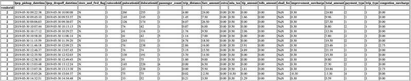
The source data is in an Amazon Redshift table. We build a forecasting ML model to predict the number of Green taxi rides in New York City.
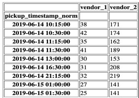
Before building the model using Amazon SageMaker DeepAR, we need to format the raw table data into a format for the algorithm to use using SQL. The following screenshot shows the original format.

The following screenshot shows the converted format.

We convert the raw table data into the preceding format by running the following SQL query. We run the UNLOAD statement using this SQL to unload the transformed data into Amazon S3.
query_str = "UNLOAD('select
   coalesce(v1.pickup_timestamp_norm, v2.pickup_timestamp_norm) as pickup_timestamp_norm,
   coalesce(v1.vendor_1, 0) as vendor_1,
   coalesce(v2.vendor_2, 0) as vendor_2
from
   (
      select
         case
            when
               extract(minute
      from
         lpep_dropoff_datetime) between 0 and 14
      then
         dateadd(minute, 0, date_trunc(''hour'', lpep_dropoff_datetime))
      when
         extract(minute
      from
         lpep_dropoff_datetime) between 15 and 29
      then
         dateadd(minute, 15, date_trunc(''hour'', lpep_dropoff_datetime))
      when
         extract(minute
      from
         lpep_dropoff_datetime) between 30 and 44
      then
         dateadd(minute, 30, date_trunc(''hour'', lpep_dropoff_datetime))
      when
         extract(minute
      from
         lpep_dropoff_datetime) between 45 and 59
      then
         dateadd(minute, 45, date_trunc(''hour'', lpep_dropoff_datetime))
         end
         as pickup_timestamp_norm , count(1) as vendor_1
      from
         taxischema.nyc_greentaxi
      where
         vendorid = 1
      group by
         1
   )
   v1
   full outer join
      (
         select
            case
               when
                  extract(minute
         from
            lpep_dropoff_datetime) between 0 and 14
         then
            dateadd(minute, 0, date_trunc(''hour'', lpep_dropoff_datetime))
         when
            extract(minute
         from
            lpep_dropoff_datetime) between 15 and 29
         then
            dateadd(minute, 15, date_trunc(''hour'', lpep_dropoff_datetime))
         when
            extract(minute
         from
            lpep_dropoff_datetime) between 30 and 44
         then
            dateadd(minute, 30, date_trunc(''hour'', lpep_dropoff_datetime))
         when
            extract(minute
         from
            lpep_dropoff_datetime) between 45 and 59
         then
            dateadd(minute, 45, date_trunc(''hour'', lpep_dropoff_datetime))
            end
            as pickup_timestamp_norm , count(1) as vendor_2
         from
            taxischema.nyc_greentaxi
         where
            vendorid = 2
         group by
            1
      )
      v2
      on v1.pickup_timestamp_norm = v2.pickup_timestamp_norm
;') to '" + redshift_unload_path + "' iam_role '" + redshift_iam_role + "' format as CSV header ALLOWOVERWRITE GZIP"
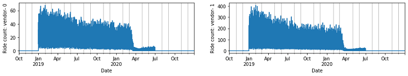
After we unload the data into Amazon S3, we load the CSV data into a Pandas DataFrame and visualize the dataset. The following plots show the number of rides aggregated per 15 minutes for each of the vendors.
We now train our model using this time series data to forecast the number of rides.
The attached Jupyter notebook contains three steps:
- Split the train and test data. Unlike classification and regression ML tasks where the train and split are done by randomly dividing the entire dataset, in this forecasting algorithm, we split the data based on time:
- Start date of training data – 2019-01-01
- End date of training data – 2020-07-31
- Train the model by setting values to the mandatory hyperparameters.
The training job takes around 15 minutes, and the training progress is displayed on the screen. When the job is complete, you see code like the following:
#metrics {"Metrics": {"model.score.time": {"count": 1, "max": 3212.099075317383, "sum": 3212.099075317383, "min": 3212.099075317383}}, "EndTime": 1597702355.281733, "Dimensions": {"Host": "algo-1", "Operation": "training", "Algorithm": "AWS/DeepAR"}, "StartTime": 1597702352.069719}

[08/17/2020 22:12:35 INFO 140060425148224] #test_score (algo-1, RMSE): 24.8660570151
[08/17/2020 22:12:35 INFO 140060425148224] #test_score (algo-1, mean_absolute_QuantileLoss): 20713.306262554062
[08/17/2020 22:12:35 INFO 140060425148224] #test_score (algo-1, mean_wQuantileLoss): 0.18868379682658334
[08/17/2020 22:12:35 INFO 140060425148224] #test_score (algo-1, wQuantileLoss[0.1]): 0.13653619964790314
[08/17/2020 22:12:35 INFO 140060425148224] #test_score (algo-1, wQuantileLoss[0.2]): 0.18786255278771358
[08/17/2020 22:12:35 INFO 140060425148224] #test_score (algo-1, wQuantileLoss[0.3]): 0.21525202142165195
[08/17/2020 22:12:35 INFO 140060425148224] #test_score (algo-1, wQuantileLoss[0.4]): 0.2283095901515685
[08/17/2020 22:12:35 INFO 140060425148224] #test_score (algo-1, wQuantileLoss[0.5]): 0.2297682531655401
[08/17/2020 22:12:35 INFO 140060425148224] #test_score (algo-1, wQuantileLoss[0.6]): 0.22057919827603453
[08/17/2020 22:12:35 INFO 140060425148224] #test_score (algo-1, wQuantileLoss[0.7]): 0.20157691985194473
[08/17/2020 22:12:35 INFO 140060425148224] #test_score (algo-1, wQuantileLoss[0.8]): 0.16576246442811773
[08/17/2020 22:12:35 INFO 140060425148224] #test_score (algo-1, wQuantileLoss[0.9]): 0.11250697170877594
[08/17/2020 22:12:35 INFO 140060425148224] #quality_metric: host=algo-1, test mean_wQuantileLoss <loss>=0.188683796827
[08/17/2020 22:12:35 INFO 140060425148224] #quality_metric: host=algo-1, test RMSE <loss>=24.8660570151
#metrics {"Metrics": {"totaltime": {"count": 1, "max": 917344.633102417, "sum": 917344.633102417, "min": 917344.633102417}, "setuptime": {"count": 1, "max": 10.606050491333008, "sum": 10.606050491333008, "min": 10.606050491333008}}, "EndTime": 1597702355.338799, "Dimensions": {"Host": "algo-1", "Operation": "training", "Algorithm": "AWS/DeepAR"}, "StartTime": 1597702355.281794}


2020-08-17 22:12:56 Uploading - Uploading generated training model
2020-08-17 22:12:56 Completed - Training job completed
Training seconds: 991
Billable seconds: 991
CPU times: user 3.48 s, sys: 210 ms, total: 3.69 s
Wall time: 18min 56s
- Deploy the trained model in an Amazon SageMaker endpoint.
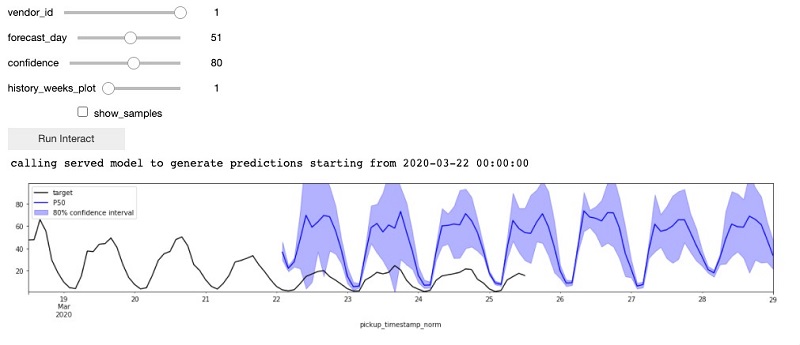
We use the endpoint to make predictions on the fly. In this post, we create an endpoint on an ml.m4.xlarge instance class. For displaying prediction results, we have provide an interactive time series graph. You can adjust four control values:
- vendor_id – The vendor ID.
- forecast_day – The offset from the training end date. This is the first date of the forecast prediction.
- confidence – The confidence interval.
- history_weeks_plot – The number of weeks in the plot prior to the forecast day.
The prediction plot looks like the following screenshot.

Conclusion
In this post, we walked through steps to interact with Amazon Redshift from an Amazon SageMaker Jupyter notebook using the Data API. We provided sample codes for the notebook to wait for the Data API to finish specific steps. The sample code showed how to configure the wait time for different SQL.
The length of wait time depends on the type of query you submit. A COPY command, which loads a large number of Amazon S3 objects, is usually longer than a SELECT query.
You can retrieve query results directly into a Pandas DataFrame by calling the GetStatementResult API. This approach simplifies the in-place analysis by delegating complex SQL queries at Amazon Redshift and visualizing the data by fetching the query result into the Jupyter notebook.
We further explored building and deploying an ML model on Amazon SageMaker using train and test data from Amazon Redshift.
For more information about the Data API, watch the video Introducing the Amazon Redshift Data API on YouTube and see Using the Amazon Redshift Data API.
About the Authors
 Saunak Chandra is a senior partner solutions architect for Redshift at AWS. Saunak likes to experiment with new products in the technology space, alongside his day to day work. He loves exploring the nature in the Pacific Northwest. A short hiking or biking in the trails is his favorite weekend morning routine. He also likes to do yoga when he gets time from his kid.
 Debu Panda, a senior product manager at AWS, is an industry leader in analytics, application platform, and database technologies. He has more than 20 years of experience in the IT industry and has published numerous articles on analytics, enterprise Java, and databases and has presented at multiple conferences. He is lead author of the EJB 3 in Action (Manning Publications 2007, 2014) and Middleware Management (Packt).
Chao Duan is a software development manager at Amazon Redshift, where he leads the development team focusing on enabling self-maintenance and self-tuning with comprehensive monitoring for Redshift. Chao is passionate about building high-availability, high-performance, and cost-effective database to empower customers with data-driven decision making.
 Saunak Chandra is a senior partner solutions architect for Redshift at AWS. Saunak likes to experiment with new products in the technology space, alongside his day to day work. He loves exploring the nature in the Pacific Northwest. A short hiking or biking in the trails is his favorite weekend morning routine. He also likes to do yoga when he gets time from his kid.
 Debu Panda, a senior product manager at AWS, is an industry leader in analytics, application platform, and database technologies. He has more than 20 years of experience in the IT industry and has published numerous articles on analytics, enterprise Java, and databases and has presented at multiple conferences. He is lead author of the EJB 3 in Action (Manning Publications 2007, 2014) and Middleware Management (Packt).
 Chao Duan is a software development manager at Amazon Redshift, where he leads the development team focusing on enabling self-maintenance and self-tuning with comprehensive monitoring for Redshift. Chao is passionate about building high-availability, high-performance, and cost-effective database to empower customers with data-driven decision making.
 data management product, which uses