Post Syndicated from Suresh Patnam original https://aws.amazon.com/blogs/big-data/part-2-migrate-a-large-data-warehouse-from-greenplum-to-amazon-redshift-using-aws-sct/
In this second post of a multi-part series, we share best practices for choosing the optimal Amazon Redshift cluster, data architecture, converting stored procedures, compatible functions and queries widely used for SQL conversions, and recommendations for optimizing the length of data types for table columns. You can check out the first post of this series for guidance on planning, running, and validation of a large-scale data warehouse migration from Greenplum to Amazon Redshift using AWS Schema Conversion Tool (AWS SCT).
Choose your optimal Amazon Redshift cluster
Amazon Redshift has two types of clusters: provisioned and serverless. For provisioned clusters, you need to set up the same with required compute resources. Amazon Redshift Serverless can run high-performance analytics in the cloud at any scale. For more information, refer to Introducing Amazon Redshift Serverless – Run Analytics At Any Scale Without Having to Manage Data Warehouse Infrastructure.
An Amazon Redshift cluster consists of nodes. Each cluster has a leader node and one or more compute nodes. The leader node receives queries from client applications, parses the queries, and develops query run plans. The leader node then coordinates the parallel run of these plans with the compute nodes and aggregates the intermediate results from these nodes. It then returns the results to the client applications.
When determining your type of cluster, consider the following:
- Estimate the size of the input data compressed, vCPU, and performance. As of this writing, we recommend the Amazon Redshift RA3 instance with managed storage, which scales compute and storage independently for fast query performance.
- Amazon Redshift provides an automated “Help me choose” cluster based on the size of your data.
- A main advantage of a cloud Amazon Redshift data warehouse is that you’re no longer stuck with hardware and commodities like old guard data warehouses. For faster innovation, you have the option to try different cluster options and choose the optimized one in terms of performance and cost.
- At the time of development or pilot, you can usually start with a smaller number of nodes. As you move to production, you can adjust the number of nodes based on your usage pattern. When right-sizing your clusters, we recommend choosing the reserved instance type to cut down the cost even further. The public-facing utility Simple Replay can help you determine performance against different cluster types and sizes by replaying the customer workload. For provisioned clusters, if you’re planning to use the recommended RA3 instance, you can compare different node types to determine the right instance type.
- Based on your workload pattern, Amazon Redshift supports resize, pause and stop, and concurrency scaling of the cluster. Amazon Redshift workload management (WLM) enables effective and flexible management of memory and query concurrency.
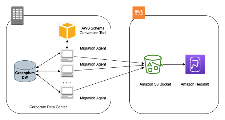
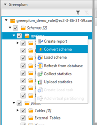
Create data extraction tasks with AWS SCT
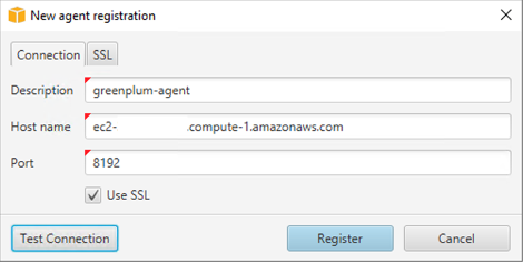
With AWS SCT extraction agents, you can migrate your source tables in parallel. These extraction agents authenticate using a valid user on the data source, allowing you to adjust the resources available for that user during the extraction. AWS SCT agents process the data locally and upload it to Amazon Simple Storage Service (Amazon S3) through the network (via AWS Direct Connect). We recommend having a consistent network bandwidth between your Greenplum machine where the AWS SCT agent is installed and your AWS Region.
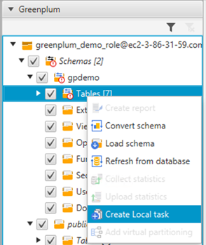
If you have tables around 20 million rows or 1 TB in size, you can use the virtual partitioning feature on AWS SCT to extract data from those tables. This creates several sub-tasks and parallelizes the data extraction process for this table. Therefore, we recommend creating two groups of tasks for each schema that you migrate: one for small tables and one for large tables using virtual partitions.
For more information, refer to Creating, running, and monitoring an AWS SCT data extraction task.
Data architecture
To simplify and modernize your data architecture, consider the following:
- Establish accountability and authority to enforce enterprise data standards and policies.
- Formalize the data and analytics operating model between enterprise and business units and functions.
- Simplify the data technology ecosystem through rationalization and modernization of data assets and tools or technology.
- Develop organizational constructs that facilitate more robust integration of the business and delivery teams, and build data-oriented products and solutions to address the business problems and opportunities throughout the lifecycle.
- Back up the data periodically so that if something is wrong, you have the ability to replay.
- During planning, design, execution, and throughout implementation and maintenance, ensure data quality management is added to achieve the desired outcome.
- Simple is the key to an easy, fast, intuitive, and low-cost solution. Simple scales much better than complex. Simple makes it possible to think big (Invent and Simplify is another Amazon leadership principle). Simplify the legacy process by migrating only the necessary data used in tables and schemas. For example, if you’re performing truncate and load for incremental data, identify a watermark and only process incremental data.
- You may have use cases that requiring record-level inserts, updates, and deletes for privacy regulations and simplified pipelines; simplified file management and near-real-time data access; or simplified change data capture (CDC) data pipeline development. We recommend using purposeful tools based on your use case. AWS offers the options to use Apache HUDI with Amazon EMR and AWS Glue.
Migrate stored procedures
In this section, we share best practices for stored procedure migration from Greenplum to Amazon Redshift. Data processing pipelines with complex business logic often use stored procedures to perform the data transformation. We advise using big data processing like AWS Glue or Amazon EMR to modernize your extract, transform, and load (ETL) jobs. For more information, check out Top 8 Best Practices for High-Performance ETL Processing Using Amazon Redshift. For time-sensitive migration to cloud-native data warehouses like Amazon Redshift, redesigning and developing the entire pipeline in a cloud-native ETL tool might be time-consuming. Therefore, migrating the stored procedures from Greenplum to Amazon Redshift stored procedures can be the right choice.
For a successful migration, make sure to follow Amazon Redshift stored procedure best practices:
- Specify the schema name while creating a stored procedure. This helps facilitate schema-level security and you can enforce grants or revoke access control.
- To prevent naming conflicts, we recommend naming procedures using the prefix
sp_. Amazon Redshift reserves thesp_prefix exclusively for stored procedures. By prefixing your procedure names withsp_, you ensure that your procedure name won’t conflict with any existing or future Amazon Redshift procedure names. - Qualify your database objects with the schema name in the stored procedure.
- Follow the minimal required access rule and revoke unwanted access. For similar implementation, make sure the stored procedure run permission is not open to ALL.
- The SECURITY attribute controls a procedure’s privileges to access database objects. When you create a stored procedure, you can set the SECURITY attribute to either DEFINER or INVOKER. If you specify SECURITY INVOKER, the procedure uses the privileges of the user invoking the procedure. If you specify SECURITY DEFINER, the procedure uses the privileges of the owner of the procedure. INVOKER is the default. For more information, refer to Security and privileges for stored procedures.
- Managing transactions when it comes to stored procedures are important. For more information, refer to Managing transactions.
- TRUNCATE issues a commit implicitly inside a stored procedure. It interferes with the transaction block by committing the current transaction and creating a new one. Exercise caution while using TRUNCATE to ensure it never breaks the atomicity of the transaction. This also applies for COMMIT and ROLLBACK.
- Adhere to cursor constraints and understand performance considerations while using cursor. You should use set-based SQL logic and temporary tables while processing large datasets.
- Avoid hardcoding in stored procedures. Use dynamic SQL to construct SQL queries dynamically at runtime. Ensure appropriate logging and error handling of the dynamic SQL.
- For exception handling, you can write RAISE statements as part of the stored procedure code. For example, you can raise an exception with a custom message or insert a record into a logging table. For unhandled exceptions like WHEN OTHERS, use built-in functions like SQLERRM or SQLSTATE to pass it on to the calling application or program. As of this writing, Amazon Redshift limits calling a stored procedure from the exception block.
Sequences
You can use IDENTITY columns, system timestamps, or epoch time as an option to ensure uniqueness. The IDENTITY column or a timestamp-based solution might have sparse values, so if you need a continuous number sequence, you need to use dedicated number tables. You can also use of the RANK() or ROW_NUMBER() window function over the entire set. Alternatively, get the high-water mark from the existing ID column from the table and increment the values while inserting records.
Character datatype length
Greenplum char and varchar data type length is specified in terms of character length, including multi-byte ones. Amazon Redshift character types are defined in terms of bytes. For table columns using multi-byte character sets in Greenplum, the converted table column in Amazon Redshift should allocate adequate storage to the actual byte size of the source data.
An easy workaround is to set the Amazon Redshift character column length to four times larger than the corresponding Greenplum column length.
A best practice is to use the smallest possible column size. Amazon Redshift doesn’t allocate storage space according to the length of the attribute; it allocates storage according to the real length of the stored string. However, at runtime, while processing queries, Amazon Redshift allocates memory according to the length of the attribute. Therefore, not setting a default size of four times greater helps from a performance perspective.
An efficient solution is to analyze production datasets and determine the maximum byte size length of the Greenplum character columns. Add a 20% buffer to support future incremental growth on the table.
To arrive at the actual byte size length of an existing column, run the Greenplum data structure character utility from the AWS Samples GitHub repo.
Numeric precision and scale
The Amazon Redshift numeric data type has a limit to store up to maximum precision of 38, whereas in a Greenplum database, you can define a numeric column without any defined length.
Analyze your production datasets and determine numeric overflow candidates using the Greenplum data structure numeric utility from the AWS Samples GitHub repo. For numeric data, you have options to tackle this based on your use case. For numbers with a decimal part, you have the option to round the data based on the data type without any data loss in the whole number part. For future reference, you can a keep copy of the column in VARCHAR or store in an S3 data lake. If you see an extremely small percentage of an outlier of overflow data, clean up the source data for quality data migration.
SQL queries and functions
While converting SQL scripts or stored procedures to Amazon Redshift, if you encounter unsupported functions, database objects, or code blocks for which you might have to rewrite the query, create user-defined functions (UDFs), or redesign. You can create a custom scalar UDF using either a SQL SELECT clause or a Python program. The new function is stored in the database and is available for any user with sufficient privileges to run. You run a custom scalar UDF in much the same way as you run existing Amazon Redshift functions to match any functionality of legacy databases. The following are some examples of alternate query statements and ways to achieve specific aggregations that might be required during a code rewrite.
AGE
The Greenplum function AGE () returns an interval subtracting from the current date. You could accomplish the same using a subset of MONTHS_BETWEEN(), ADD_MONTH(), DATEDIFF(), and TRUNC() functions based on your use case.
The following example Amazon Redshift query calculates the gap between the date 2001-04-10 and 1957-06-13 in terms of year, month, and days. You can apply this to any date column in a table.

COUNT
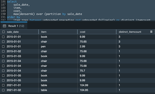
If you have a use case to get distinct aggregation in the Count() window function, you could accomplish the same using a combination of the Dense_Rank () and Max() window functions.
The following example Amazon Redshift query calculates the distinct item count for a given date of sale:
ORDER BY
Amazon Redshift aggregate window functions with an ORDER BY clause require a mandatory frame.
The following example Amazon Redshift query creates a cumulative sum of cost by sale date and orders the results by item within the partition:

STRING_AGG
In Greenplum, STRING_AGG() is an aggregate function, which is used to concatenate a list of strings. In Amazon Redshift, use the LISTAGG() function.
The following example Amazon Redshift query returns a semicolon-separated list of email addresses for each department:

ARRAY_AGG
In Greenplum, ARRAY_AGG() is an aggregate function that takes a set of values as input and returns an array. In Amazon Redshift, use a combination of the LISTAGG() and SPLIT_TO_ARRAY() functions. The SPLIT_TO_ARRAY() function returns a SUPER datatype.
The following example Amazon Redshift query returns an array of email addresses for each department:

To retrieve array elements from a SUPER expression, you can use the SUBARRAY() function:

UNNEST
In Greenplum, you can use the UNNEST function to split an array and convert the array elements into a set of rows. In Amazon Redshift, you can use PartiQL syntax to iterate over SUPER arrays. For more information, refer to Querying semistructured data.

WHERE
You can’t use a window function in the WHERE clause of a query in Amazon Redshift. Instead, construct the query using the WITH clause and then refer the calculated column in the WHERE clause.
The following example Amazon Redshift query returns the sale date, item, and cost from a table for the sales dates where the total sale is more than 100:

Refer to the following table for additional Greenplum date/time functions along with the Amazon Redshift equivalent to accelerate you code migration.
| . | Description | Greenplum | Amazon Redshift |
| 1 | The now() function return the start time of the current transaction |
now () |
sysdate |
| 2 | clock_timestamp() returns the start timestamp of the current statement within a transaction block |
clock_timestamp () |
to_date(getdate(),'yyyy-mm-dd') + substring(timeofday(),12,15)::timetz |
| 3 | transaction_timestamp () returns the start timestamp of the current transaction |
transaction_timestamp () |
to_date(getdate(),'yyyy-mm-dd') + substring(timeofday(),12,15)::timetz |
| 4 | Interval – This function adds x years and y months to the date_time_column and returns a timestamp type |
date_time_column + interval ‘ x years y months’ |
add_months(date_time_column, x*12 + y) |
| 5 | Get total number of seconds between two-time stamp fields | date_part('day', end_ts - start_ts) * 24 * 60 * 60+ date_part('hours', end_ts - start_ts) * 60 * 60+ date_part('minutes', end_ts - start_ts) * 60+ date_part('seconds', end_ts - start_ts) |
datediff('seconds', start_ts, end_ts) |
| 6 | Get total number of minutes between two-time stamp fields | date_part('day', end_ts - start_ts) * 24 * 60 + date_part('hours', end_ts - start_ts) * 60 + date_part('minutes', end_ts - start_ts) |
datediff('minutes', start_ts, end_ts) |
| 7 | Extract date part literal from difference of two-time stamp fields | date_part('hour', end_ts - start_ts) |
extract(hour from (date_time_column_2 - date_time_column_1)) |
| 8 | Function to return the ISO day of the week | date_part('isodow', date_time_column) |
TO_CHAR(date_time_column, 'ID') |
| 9 | Function to return ISO year from date time field | extract (isoyear from date_time_column) |
TO_CHAR(date_time_column, ‘IYYY’) |
| 10 | Convert epoch seconds to equivalent datetime | to_timestamp(epoch seconds) |
TIMESTAMP 'epoch' + Number_of_seconds * interval '1 second' |
Amazon Redshift utility for troubleshooting or running diagnostics for the cluster
The Amazon Redshift Utilities GitHub repo contains a set of utilities to accelerate troubleshooting or analysis on Amazon Redshift. Such utilities consist of queries, views, and scripts. They are not deployed by default onto Amazon Redshift clusters. The best practice is to deploy the needed views into the admin schema.
Conclusion
In this post, we covered prescriptive guidance around data types, functions, and stored procedures to accelerate the migration process from Greenplum to Amazon Redshift. Although this post describes modernizing and moving to a cloud warehouse, you should be augmenting this transformation process towards a full-fledged modern data architecture. The AWS Cloud enables you to be more data-driven by supporting multiple use cases. For a modern data architecture, you should use purposeful data stores like Amazon S3, Amazon Redshift, Amazon Timestream, and others based on your use case.
About the Authors
 Suresh Patnam is a Principal Solutions Architect at AWS. He is passionate about helping businesses of all sizes transforming into fast-moving digital organizations focusing on big data, data lakes, and AI/ML. Suresh holds a MBA degree from Duke University- Fuqua School of Business and MS in CIS from Missouri State University. In his spare time, Suresh enjoys playing tennis and spending time with his family.
 Arunabha Datta is a Sr. Data Architect at AWS Professional Services. He collaborates with customers and partners to architect and implement modern data architecture using AWS Analytics services. In his spare time, Arunabha enjoys photography and spending time with his family.