Post Syndicated from Ahmed Shehata original https://aws.amazon.com/blogs/big-data/migrate-microsoft-azure-synapse-analytics-to-amazon-redshift-using-aws-sct/
Amazon Redshift is a fast, fully managed, petabyte-scale data warehouse that provides the flexibility to use provisioned or serverless compute for your analytical workloads. With Amazon Redshift Serverless and Query Editor v2, you can load and query large datasets in just a few clicks and pay only for what you use. The decoupled compute and storage architecture of Amazon Redshift enables you to build highly scalable, resilient, and cost-effective workloads. Many customers migrate their data warehousing workloads to Amazon Redshift and benefit from the rich capabilities it offers, such as the following:
- Amazon Redshift seamlessly integrates with broader data, analytics, and AI or machine learning (ML) services on AWS, enabling you to choose the right tool for the right job. Modern analytics is much wider than SQL-based data warehousing. With Amazon Redshift, you can build lake house architectures and perform any kind of analytics, such as interactive analytics, operational analytics, big data processing, visual data preparation, predictive analytics, machine learning, and more.
- You don’t need to worry about workloads such as ETL (extract, transform, and load), dashboards, ad-hoc queries, and so on interfering with each other. You can isolate workloads using data sharing, while using the same underlying datasets.
- When users run many queries at peak times, compute seamlessly scales within seconds to provide consistent performance at high concurrency. You get 1 hour of free concurrency scaling capacity for 24 hours of usage. This free credit meets the concurrency demand of 97% of the Amazon Redshift customer base.
- Amazon Redshift is straightforward to use with self-tuning and self-optimizing capabilities. You can get faster insights without spending valuable time managing your data warehouse.
- Fault tolerance is built in. All data written to Amazon Redshift is automatically and continuously replicated to Amazon Simple Storage Service (Amazon S3). Any hardware failures are automatically replaced.
- Amazon Redshift is simple to interact with. You can access data with traditional, cloud-native, containerized, serverless web services or event-driven applications. You can also use your favorite business intelligence (BI) and SQL tools to access, analyze, and visualize data in Amazon Redshift.
- Amazon Redshift ML makes it straightforward for data scientists to create, train, and deploy ML models using familiar SQL. You can also run predictions using SQL.
- Amazon Redshift provides comprehensive data security at no extra cost. You can set up end-to-end data encryption, configure firewall rules, define granular row-level and column-level security controls on sensitive data, and more.
In this post, we show how to migrate a data warehouse from Microsoft Azure Synapse to Redshift Serverless using AWS Schema Conversion Tool (AWS SCT) and AWS SCT data extraction agents. AWS SCT makes heterogeneous database migrations predictable by automatically converting the source database code and storage objects to a format compatible with the target database. Any objects that can’t be automatically converted are clearly marked so that they can be manually converted to complete the migration. AWS SCT can also scan your application code for embedded SQL statements and convert them.
Solution overview
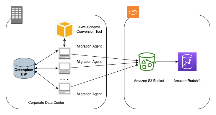
AWS SCT uses a service account to connect to your Azure Synapse Analytics. First, we create a Redshift database into which Azure Synapse data will be migrated. Next, we create an S3 bucket. Then, we use AWS SCT to convert Azure Synapse schemas and apply them to Amazon Redshift. Finally, to migrate data, we use AWS SCT data extraction agents, which extract data from Azure Synapse, upload it into an S3 bucket, and copy it to Amazon Redshift.
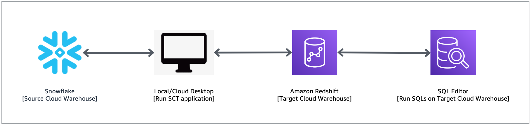
The following diagram illustrates our solution architecture.

This walkthrough covers the following steps:
- Create a Redshift Serverless data warehouse.
- Create the S3 bucket and folder.
- Convert and apply the Azure Synapse schema to Amazon Redshift using AWS SCT:
- Connect to the Azure Synapse source.
- Connect to the Amazon Redshift target.
- Convert the Azure Synapse schema to a Redshift database.
- Analyze the assessment report and address the action items.
- Apply the converted schema to the target Redshift database.
- Migrate data from Azure Synapse to Amazon Redshift using AWS SCT data extraction agents:
- Generate trust and key stores (this step is optional).
- Install and configure the data extraction agent.
- Start the data extraction agent.
- Register the data extraction agent.
- Add virtual partitions for large tables (this step is optional).
- Create a local data migration task.
- Start the local data migration task.
- View data in Amazon Redshift.
Prerequisites
Before starting this walkthrough, you must have the following prerequisites:
- A workstation with AWS SCT, Amazon Corretto 11, and Redshift drivers.
- You can use an Amazon Elastic Compute Cloud (Amazon EC2) instance or your local desktop as a workstation. In this walkthrough, we use an Amazon EC2 Windows instance. To create it, refer to Tutorial: Get started with Amazon EC2 Windows instances.
- To download and install AWS SCT on the EC2 instance that you created, refer to Installing, verifying, and updating AWS SCT.
- Download the Redshift JDBC driver.
- Download and install Amazon Corretto 11.
- A database user account that AWS SCT can use to connect to your source Azure Synapse Analytics database.
- Grant VIEW DEFINITION and VIEW DATABASE STATE to each schema you are trying to convert to the database user used for migration.
Create a Redshift Serverless data warehouse
In this step, we create a Redshift Serverless data warehouse with a workgroup and namespace. A workgroup is a collection of compute resources and a namespace is a collection of database objects and users. To isolate workloads and manage different resources in Redshift Serverless, you can create namespaces and workgroups and manage storage and compute resources separately.
Follow these steps to create a Redshift Serverless data warehouse with a workgroup and namespace:
- On the Amazon Redshift console, choose the AWS Region that you want to use.
- In the navigation pane, choose Redshift Serverless.
- Choose Create workgroup.

- For Workgroup name, enter a name that describes the compute resources.

- Verify that the VPC is the same as the VPC as the EC2 instance with AWS SCT.
- Choose Next.
- For Namespace, enter a name that describes your dataset.
- In the Database name and password section, select Customize admin user credentials.
- For Admin user name, enter a user name of your choice (for example,
awsuser). - For Admin user password, enter a password of your choice (for example,
MyRedShiftPW2022).

- Choose Next.
Note that data in the Redshift Serverless namespace is encrypted by default.
- In the Review and Create section, choose Create.
Now you create an AWS Identity and Access Management (IAM) role and set it as the default on your namespace. Note that there can only be one default IAM role.
- On the Redshift Serverless Dashboard, in the Namespaces / Workgroups section, choose the namespace you just created.
- On the Security and encryption tab, in the Permissions section, choose Manage IAM roles.
- Choose Manage IAM roles and choose Create IAM role.
- In the Specify an Amazon S3 bucket for the IAM role to access section, choose one of the following methods:
- Choose No additional Amazon S3 bucket to allow the created IAM role to access only the S3 buckets with names containing the word redshift.
- Choose Any Amazon S3 bucket to allow the created IAM role to access all S3 buckets.
- Choose Specific Amazon S3 buckets to specify one or more S3 buckets for the created IAM role to access. Then choose one or more S3 buckets from the table.
- Choose Create IAM role as default.
- Capture the endpoint for the Redshift Serverless workgroup you just created.
- On the Redshift Serverless Dashboard, in the Namespaces / Workgroups section, choose the workgroup you just created.
- In the General information section, copy the endpoint.
Create the S3 bucket and folder
During the data migration process, AWS SCT uses Amazon S3 as a staging area for the extracted data. Follow these steps to create an S3 bucket:
- On the Amazon S3 console, choose Buckets in the navigation pane.
- Choose Create bucket.
- For Bucket name, enter a unique DNS-compliant name for your bucket (for example,
uniquename-as-rs).
For more information about bucket names, refer to Bucket naming rules.
- For AWS Region, choose the Region in which you created the Redshift Serverless workgroup.
- Choose Create bucket.

- Choose Buckets in the navigation pane and navigate to the S3 bucket you just created (
uniquename-as-rs). - Choose Create folder.
- For Folder name, enter incoming.
- Choose Create folder.
Convert and apply the Azure Synapse schema to Amazon Redshift using AWS SCT
To convert the Azure Synapse schema to Amazon Redshift format, we use AWS SCT. Start by logging in to the EC2 instance that you created previously and launch AWS SCT.
Connect to the Azure Synapse source
Complete the following steps to connect to the Azure Synapse source:
- On the File menu, choose Create New Project.
- Choose a location to store your project files and data.
- Provide a meaningful but memorable name for your project (for example, Azure Synapse to Amazon Redshift).
- To connect to the Azure Synapse source data warehouse, choose Add source.
- Choose Azure Synapse and choose Next.
- For Connection name, enter a name (for example,
olap-azure-synapse).
AWS SCT displays this name in the object tree in left pane.
- For Server name, enter your Azure Synapse server name.
- For SQL pool, enter your Azure Synapse pool name.
- Enter a user name and password.
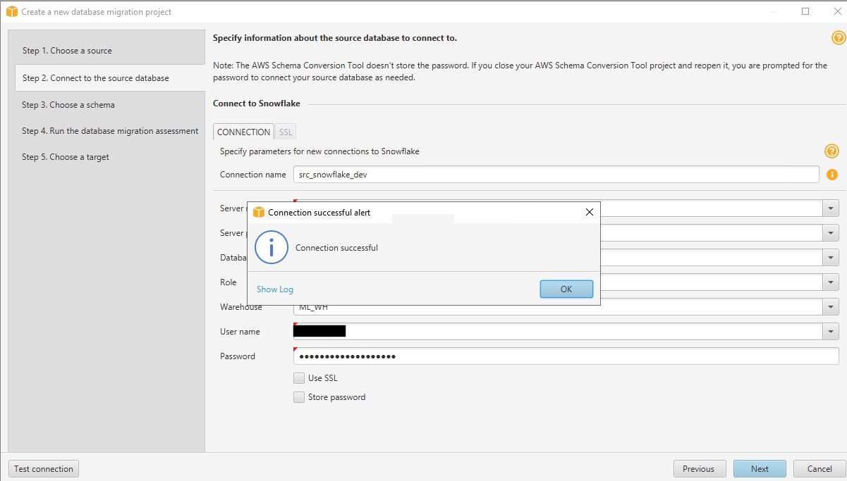
- Choose Test connection to verify that AWS SCT can connect to your source Azure Synapse project.
- When the connection is successfully validated, choose Ok and Connect.

Connect to the Amazon Redshift target
Follow these steps to connect to Amazon Redshift:
- In AWS SCT, choose Add target.
- Choose Amazon Redshift, then choose Next.
- For Connection name, enter a name to describe the Amazon Redshift connection.
AWS SCT displays this name in the object tree in the right pane.
- For Server name, enter the Redshift Serverless workgroup endpoint you captured earlier.
- For Server port, enter 5439.
- For Database, enter dev.
- For User name, enter the user name you chose when creating the Redshift Serverless workgroup.
- For Password, enter the password you chose when creating the Redshift Serverless workgroup.
- Deselect Use AWS Glue.
- Choose Test connection to verify that AWS SCT can connect to your target Redshift workgroup.
- When the test is successful, choose OK.
- Choose Connect to connect to the Amazon Redshift target.
Alternatively, you can use connection values that are stored in AWS Secrets Manager.

Convert the Azure Synapse schema to a Redshift data warehouse
After you create the source and target connections, you will see the source Azure Synapse object tree in the left pane and the target Amazon Redshift object tree in the right pane. We then create mapping rules to describe the source target pair for the Azure Synapse to Amazon Redshift migration.
Follow these steps to convert the Azure Synapse dataset to Amazon Redshift format:
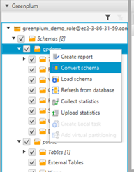
- In the left pane, choose (right-click) the schema you want to convert.
- Choose Convert schema.
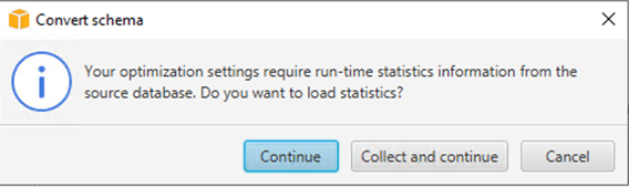
- In the dialog box, choose Yes.
When the conversion is complete, you will see a new schema created in the Amazon Redshift pane (right pane) with the same name as your Azure Synapse schema.

The sample schema we used has three tables; you can see these objects in Amazon Redshift format in the right pane. AWS SCT converts all the Azure Synapse code and data objects to Amazon Redshift format. You can also use AWS SCT to convert external SQL scripts, application code, or additional files with embedded SQL.
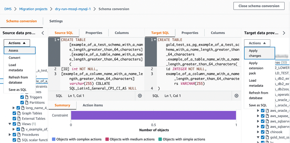
Analyze the assessment report and address the action items
AWS SCT creates an assessment report to assess the migration complexity. AWS SCT can convert the majority of code and database objects, but some objects may require manual conversion. AWS SCT highlights these objects in blue in the conversion statistics diagram and creates action items with a complexity attached to them.
To view the assessment report, switch from Main view to Assessment Report view as shown in the following screenshot.

The Summary tab shows objects that were converted automatically and objects that were not converted automatically. Green represents automatically converted objects or objects with simple action items. Blue represents medium and complex action items that require manual intervention.

The Action items tab shows the recommended actions for each conversion issue. If you choose an action item from the list, AWS SCT highlights the object that the action item applies to.

The report also contains recommendations for how to manually convert the schema item. For example, after the assessment runs, detailed reports for the database and schema show you the effort required to design and implement the recommendations for converting action items. For more information about deciding how to handle manual conversions, see Handling manual conversions in AWS SCT. AWS SCT completes some actions automatically while converting the schema to Amazon Redshift; objects with such actions are marked with a red warning sign.

You can evaluate and inspect the individual object DDL by selecting it in the right pane, and you can also edit it as needed. In the following example, AWS SCT modifies the ID column data type from decimal(3,0) in Azure Synapse to the smallint data type in Amazon Redshift.
Apply the converted schema to the target Redshift data warehouse
To apply the converted schema to Amazon Redshift, select the converted schema in the right pane, right-click, and choose Apply to database.

Migrate data from Azure Synapse to Amazon Redshift using AWS SCT data extraction agents
AWS SCT extraction agents extract data from your source database and migrate it to the AWS Cloud. In this section, we configure AWS SCT extraction agents to extract data from Azure Synapse and migrate to Amazon Redshift. For this post, we install the AWS SCT extraction agent on the same Windows instance that has AWS SCT installed. For better performance, we recommend that you use a separate Linux instance to install extraction agents if possible. For very large datasets, AWS SCT supports the use of multiple data extraction agents running on several instances to maximize throughput and increase the speed of data migration.
Generate trust and key stores (optional)
You can use Secure Socket Layer (SSL) encrypted communication with AWS SCT data extractors. When you use SSL, all data passed between the applications remains private and integral. To use SSL communication, you need to generate trust and key stores using AWS SCT. You can skip this step if you don’t want to use SSL. We recommend using SSL for production workloads.
Follow these steps to generate trust and key stores:
- In AWS SCT, choose Settings, Global settings, and Security.
- Choose Generate trust and key store.

- Enter a name and password for the trust and key stores.
- Enter a location to store them.
- Choose Generate, then choose OK.

Install and configure the data extraction agent
In the installation package for AWS SCT, you can find a subfolder called agents (\aws-schema-conversion-tool-1.0.latest.zip\agents). Locate and install the executable file with a name like aws-schema-conversion-tool-extractor-xxxxxxxx.msi.

In the installation process, follow these steps to configure AWS SCT Data Extractor:
- For Service port, enter the port number the agent listens on. It is 8192 by default.
- For Working folder, enter the path where the AWS SCT data extraction agent will store the extracted data.
The working folder can be on a different computer from the agent, and a single working folder can be shared by multiple agents on different computers.
- For Enter Redshift JDBC driver file or files, enter the location where you downloaded the Redshift JDBC drivers.
- For Add the Amazon Redshift driver, enter
YES. - For Enable SSL communication, enter
yes. EnterNohere if you don’t want to use SSL. - Choose Next.

- For Trust store path, enter the storage location you specified when creating the trust and key store.
- For Trust store password, enter the password for the trust store.
- For Enable client SSL authentication, enter
yes. - For Key store path, enter the storage location you specified when creating the trust and key store.
- For Key store password, enter the password for the key store.
- Choose Next.

Start the data extraction agent
Use the following procedure to start extraction agents. Repeat this procedure on each computer that has an extraction agent installed.
Extraction agents act as listeners. When you start an agent with this procedure, the agent starts listening for instructions. You send the agents instructions to extract data from your data warehouse in a later section.
To start the extraction agent, navigate to the AWS SCT Data Extractor Agent directory. For example, in Microsoft Windows, use C:\Program Files\AWS SCT Data Extractor Agent\StartAgent.bat.
On the computer that has the extraction agent installed, from a command prompt or terminal window, run the command listed for your operating system. To stop an agent, run the same command but replace start with stop. To restart an agent, run the same RestartAgent.bat file.
Note that you should have administrator access to run those commands.

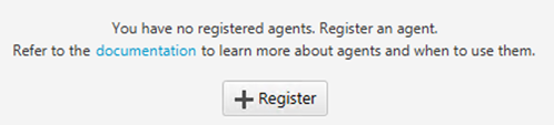
Register the data extraction agent
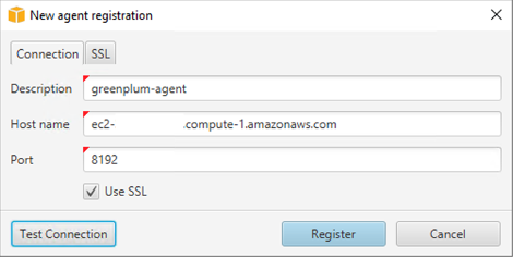
Follow these steps to register the data extraction agent:
- In AWS SCT, change the view to Data Migration view choose Register.
- Select Redshift data agent, then choose OK.

- For Description, enter a name to identify the agent.
- For Host name, if you installed the extraction agent on the same workstation as AWS SCT, enter 0.0.0.0 to indicate local host. Otherwise, enter the host name of the machine on which the AWS SCT extraction agent is installed. It is recommended to install extraction agents on Linux for better performance.
- For Port, enter the number you used for the listening port (default 8192) when installing the AWS SCT extraction agent.
- Select Use SSL to encrypt AWS SCT connection to Data Extraction Agent.

- If you’re using SSL, navigate to the SSL tab.
- For Trust store, choose the trust store you created earlier.
- For Key store, choose the key store you created earlier.
- Choose Test connection.
- After the connection is validated successfully, choose OK and Register.

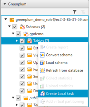
Create a local data migration task
To migrate data from Azure Synapse Analytics to Amazon Redshift, you create, run, and monitor the local migration task from AWS SCT. This step uses the data extraction agent to migrate data by creating a task.
Follow these steps to create a local data migration task:
- In AWS SCT, under the schema name in the left pane, choose (right-click) the table you want to migrate (for this post, we use the table
tbl_currency). - Choose Create Local task.

- Choose from the following migration modes:
- Extract the source data and store it on a local PC or virtual machine where the agent runs.
- Extract the data and upload it to an S3 bucket.
- Extract the data, upload it to Amazon S3, and copy it into Amazon Redshift. (We choose this option for this post.)

- On the Advanced tab, provide the extraction and copy settings.

- On the Source server tab, make sure you are using the current connection properties.

- On the Amazon S3 settings tab, for Amazon S3 bucket folder, provide the bucket and folder names of the S3 bucket you created earlier.
The AWS SCT data extraction agent uploads the data in those S3 buckets and folders before copying it to Amazon Redshift.
- Choose Test Task.

- When the task is successfully validated, choose OK, then choose Create.

Start the local data migration task
To start the task, choose Start or Restart on the Tasks tab.

First, the data extraction agent extracts data from Azure Synapse. Then the agent uploads data to Amazon S3 and launches a copy command to move the data to Amazon Redshift.
At this point, AWS SCT has successfully migrated data from the source Azure Synapse table to the Redshift table.

View data in Amazon Redshift
After the data migration task is complete, you can connect to Amazon Redshift and validate the data. Complete the following steps:
- On the Amazon Redshift console, navigate to the Query Editor v2.
- Open the Redshift Serverless workgroup you created.
- Choose Query data.

- For Database, enter a name for your database.
- For Authentication, select Federated user
- Choose Create connection.

- Open a new editor by choosing the plus sign.
- In the editor, write a query to select from the schema name and table or view name you want to verify.
You can explore the data, run ad-hoc queries, and make visualizations, charts, and views.

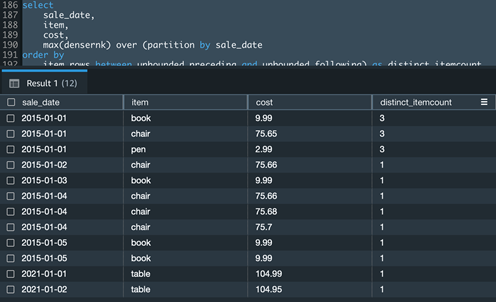
The following screenshot is the view of the source Azure Synapse dataset we used in this post.

Clean up
Follow the steps in this section to clean up any AWS resources you created as part of this post.
Stop the EC2 instance
Follow these steps to stop the EC2 instance:
- On the Amazon EC2 console, in the navigation pane, choose Instances.
- Select the instance you created.
- Choose Instance state, then choose Terminate instance.
- Choose Terminate when prompted for confirmation.
Delete the Redshift Serverless workgroup and namespace
Follow these steps to delete the Redshift Serverless workgroup and namespace:
- On the Redshift Serverless Dashboard, in the Namespaces / Workgroups section, choose the workspace you created
- On the Actions menu, choose Delete workgroup.
- Select Delete the associated namespace.
- Deselect Create final snapshot.
- Enter delete in the confirmation text box and choose Delete.
Delete the S3 bucket
Follow these steps to delete the S3 bucket:
- On the Amazon S3 console, choose Buckets in the navigation pane.
- Choose the bucket you created.
- Choose Delete.
- To confirm deletion, enter the name of the bucket.
- Choose Delete bucket.
Conclusion
Migrating a data warehouse can be a challenging, complex, and yet rewarding project. AWS SCT reduces the complexity of data warehouse migrations. This post discussed how a data migration task extracts, downloads, and migrates data from Azure Synapse to Amazon Redshift. The solution we presented performs a one-time migration of database objects and data. Data changes made in Azure Synapse when the migration is in progress won’t be reflected in Amazon Redshift. When data migration is in progress, put your ETL jobs to Azure Synapse on hold or rerun the ETL jobs by pointing to Amazon Redshift after the migration. Consider using the best practices for AWS SCT.
To get started, download and install AWS SCT, sign in to the AWS Management Console, check out Redshift Serverless, and start migrating!
About the Authors
 Ahmed Shehata is a Senior Analytics Specialist Solutions Architect at AWS based on Toronto. He has more than two decades of experience helping customers modernize their data platforms. Ahmed is passionate about helping customers build efficient, performant, and scalable analytic solutions.
 Jagadish Kumar is a Senior Analytics Specialist Solutions Architect at AWS focused on Amazon Redshift. He is deeply passionate about Data Architecture and helps customers build analytics solutions at scale on AWS.
 Anusha Challa is a Senior Analytics Specialist Solution Architect at AWS focused on Amazon Redshift. She has helped many customers build large-scale data warehouse solutions in the cloud and on premises. Anusha is passionate about data analytics and data science and enabling customers achieve success with their large-scale data projects.


 Mykhailo Kondak is a Database Engineer in the AWS Database Migration Service team at AWS. He uses his experience with different database technologies to help Amazon customers to move their on-premises data warehouses and big data workloads to the AWS Cloud. In his spare time, he plays soccer.
 Illia Kravtsov is a Database Engineer on the AWS Database Migration Service team. He has over 10 years of experience in data warehouse development with Teradata and other massively parallel processing (MPP) databases.
 Michael Soo is a Principal Database Engineer in the AWS Database Migration Service. He builds products and services that help customers migrate their database workloads to the AWS Cloud.


 Choose Create instance profile and specify your default VPC or a new VPC,


 Michael Soo is a Principal Database Engineer with the AWS Database Migration Service team. He builds products and services that help customers migrate their database workloads to the AWS cloud.
 Illia Kravtsov is a Database Developer with the AWS Project Delta Migration team. He has 10+ years experience in data warehouse development with Teradata and other MPP databases.