All posts by Tomohiro Tanaka

Introducing Apache Iceberg materialized views in AWS Glue Data Catalog

Post Syndicated from Tomohiro Tanaka original https://aws.amazon.com/blogs/big-data/introducing-apache-iceberg-materialized-views-in-aws-glue-data-catalog/

Hundreds of thousands of customers build artificial intelligence and machine learning (AI/ML) and analytics applications on AWS, frequently transforming data through multiple stages for improved query performance—from raw data to processed datasets to final analytical tables. Data engineers must solve complex problems, including detecting what data has changed in base tables, writing and maintaining transformation logic, scheduling and orchestrating workflows across dependencies, provisioning and managing compute infrastructure, and troubleshooting failures while monitoring pipeline health. Consider an ecommerce company where data engineers need to continuously merge clickstream logs with orders data for analytics. Each transformation requires building robust change detection mechanisms, writing complex joins and aggregations, coordinating multiple workflow steps, scaling compute resources appropriately, and maintaining operational oversight—all while supporting data quality and pipeline reliability. This complexity demands months of dedicated engineering effort and ongoing maintenance, making data transformation costly and time-intensive for organizations seeking to unlock insights from their data.

To address those challenges, AWS announced a new materialized view capability for Apache Iceberg tables in the AWS Glue Data Catalog. The new materialized view capability simplifies data pipelines and accelerates data lake query performance. A materialized view is a managed table in the AWS Glue Data Catalog that stores pre-computed results of a query in Iceberg format that is incrementally updated to reflect changes to the underlying datasets. This alleviates the need to build and maintain complex data pipelines to generate transformed datasets and accelerate query performance. Apache Spark engines across Amazon Athena, Amazon EMR, and AWS Glue support the new materialized views and intelligently rewrite queries to use materialized views that speed up performance while reducing compute costs.

In this post, we show you how Iceberg materialized view works and how to get started.

How Iceberg materialized views work

Iceberg materialized views offer a simple, managed solution built on familiar SQL syntax. Instead of building complex pipelines, you can create materialized views using standard SQL queries from Spark, transforming data with aggregates, filters, and joins without writing custom data pipelines. Change detection, incremental updates, and monitoring source tables are automatically handled in the AWS Glue Data Catalog and refreshing materialized views as new data arrive, alleviating the need for manual pipeline orchestration. Data transformations run on fully managed compute infrastructure, removing the burden of provisioning, scaling, or maintaining servers.

The resulting pre-computed data is stored as Iceberg tables in an Amazon Simple Storage Service (Amazon S3) general purpose bucket, or Amazon S3 Tables buckets within the your account, making transformed data immediately accessible to multiple query engines, including Athena, Amazon Redshift, and AWS optimized Spark runtime. Spark engines across Athena, Amazon EMR, and AWS Glue support an automatic query rewrite functionality that intelligently uses materialized views, delivering automatic performance improvement for data processing jobs or interactive notebook queries.

In the following sections, we walk through the steps to create, query, and refresh materialized views.

Pre-requisite

To follow along with this post, you must have an AWS account.

To run the instruction on Amazon EMR, complete the following steps to configure the cluster:

  1. Launch an Amazon EMR cluster 7.12.0 or higher.
  2. SSH login to the primary node of your Amazon EMR cluster, and run the following command to start a Spark application with required configurations:
    spark-sql \
      --conf spark.sql.extensions=org.apache.iceberg.spark.extensions.IcebergSparkSessionExtensions \
      --conf spark.sql.catalog.glue_catalog=org.apache.iceberg.spark.SparkCatalog \
      --conf spark.sql.catalog.glue_catalog.type=glue \
      --conf spark.sql.catalog.glue_catalog.warehouse=s3://amzn-s3-demo-bucket/warehouse \
      --conf spark.sql.catalog.glue_catalog.glue.region=us-east-1 \
      --conf spark.sql.catalog.glue_catalog.glue.id=123456789012 \
      --conf spark.sql.catalog.glue_catalog.glue.account-id=123456789012 \
      --conf spark.sql.catalog.glue_catalog.client.region=us-east-1 \
      --conf spark.sql.catalog.glue_catalog.glue.lakeformation-enabled=true \
      --conf spark.sql.optimizer.answerQueriesWithMVs.enabled=true \
      --conf spark.sql.defaultCatalog=glue_catalog
      

To run the instruction on AWS Glue for Spark, complete the following steps to configure the job:

  1. Create an AWS Glue version 5.1 job or higher.
  2. Configure a job parameter
    1. Key: --conf
    2. Value: spark.sql.extensions=org.apache.iceberg.spark.extensions.IcebergSparkSessionExtensions
  3. Configure your job with the following script:
    from pyspark.sql import SparkSession
    
    
    spark = (
        SparkSession.builder \
            .config("spark.sql.extensions", "org.apache.iceberg.spark.extensions.IcebergSparkSessionExtensions")
            .config("spark.sql.catalog.glue_catalog", "org.apache.iceberg.spark.SparkCatalog")
            .config("spark.sql.catalog.glue_catalog.type", "glue")
            .config("spark.sql.catalog.glue_catalog.warehouse", "s3://amzn- -demo-bucket/warehouse")
            .config("spark.sql.catalog.glue_catalog.glue.region", "us-east-1")
            .config("spark.sql.catalog.glue_catalog.glue.id", "123456789012")
            .config("spark.sql.catalog.glue_catalog.glue.account-id", "123456789012")
    		.config("spark.sql.catalog.glue_catalog.client.region", "us-east-1")
            .config("spark.sql.catalog.glue_catalog.glue.lakeformation-enabled", "true")
            .config("spark.sql.optimizer.answerQueriesWithMVs.enabled", "true")
            .config("spark.sql.defaultCatalog", "glue_catalog")
            .getOrCreate()
    )

  4. Run the following queries using Spark SQL to set up a base table. In AWS Glue, you can run them through spark.sql("QUERY STATEMENT").
    CREATE DATABASE IF NOT EXIST iceberg_mv;
    
    USE iceberg_mv;
    
    CREATE TABLE IF NOT EXISTS base_tbl (
        id INT,
        customer_name STRING,
        amount INT,
        order_date DATE);
        
    INSERT INTO base_tbl VALUES (1, 'John Doe', 150, DATE('2025-12-01')), (2, 'Jane Smith', 200, DATE('2025-12-02')), (3, 'Bob Johnson', 75, DATE('2025-12-03'));
    
    SELECT * FROM base_tbl;

In the subsequent sections, we create a materialized view with this base table.

If you want to store your materialized views in Amazon S3 Tables instead of a general Amazon S3 bucket, refer to Appendix 1 at the end of this post for the configuration details.

Create a materialized view

To create a materialized view, run the following command:

CREATE MATERIALIZED VIEW mv
AS SELECT
    customer_name, 
    COUNT(*) as mv_order_count, 
    SUM(amount) as mv_total_amount 
FROM glue_catalog.iceberg_mv.base_tbl
GROUP BY customer_name;

After you create a materialized view, AWS Spark’s in-memory metadata cache needs time to populate with information about the new materialized view. During this cache population period, queries against the base table will run normally without using the materialized view. After the cache is fully populated (typically within tens of seconds), Spark automatically detects that the materialized view can satisfy the query and rewrites it to use the pre-computed materialized view instead, improving performance.

To see this behavior, run the following EXPLAIN command immediately after creating the materialized view:

EXPLAIN EXTENDED
SELECT customer_name, COUNT(*) as mv_order_count, SUM(amount) as mv_total_amount 
FROM base_tbl
GROUP BY customer_name;

The following output shows the initial result before cache population:

== Parsed Logical Plan ==
'Aggregate ['customer_name], ['customer_name, 'COUNT(1) AS mv_order_count#0, 'SUM('amount) AS mv_total_amount#1]
+- 'UnresolvedRelation [base_tbl] , [], false

== Analyzed Logical Plan ==
customer_name: string, mv_order_count: bigint, mv_total_amount: bigint
Aggregate [customer_name#8], [customer_name#8, count(1) AS mv_order_count#0L, sum(amount#9) AS mv_total_amount#1L]
+- SubqueryAlias glue_catalog.iceberg_mv.base_tbl
   +- RelationV2[id#7, customer_name#8, amount#9, order_date#10] glue_catalog.iceberg_mv.base_tbl glue_catalog.iceberg_mv.base_tbl

== Optimized Logical Plan ==
Aggregate [customer_name#8], [customer_name#8, count(1) AS mv_order_count#0L, sum(amount#9) AS mv_total_amount#1L]
+- RelationV2[customer_name#8, amount#9] glue_catalog.iceberg_mv.base_tbl

== Physical Plan ==
AdaptiveSparkPlan isFinalPlan=false
+- HashAggregate(keys=[customer_name#8], functions=[count(1), sum(amount#9)], output=[customer_name#8, mv_order_count#0L, mv_total_amount#1L], schema specialized)
   +- Exchange hashpartitioning(customer_name#8, 1000), ENSURE_REQUIREMENTS, [plan_id=19]
      +- HashAggregate(keys=[customer_name#8], functions=[partial_count(1), partial_sum(amount#9)], output=[customer_name#8, count#27L, sum#29L], schema specialized)
         +- BatchScan glue_catalog.iceberg_mv.base_tbl[customer_name#8, amount#9] glue_catalog.iceberg_mv.base_tbl (branch=null) [filters=, groupedBy=, pushedLimit=None] RuntimeFilters: []

In this initial execution plan, Spark scans the base_tbl directly (BatchScan glue_catalog.iceberg_mv.base_tbl) and runs aggregations (COUNT and SUM) on the raw data. This is the behavior before the materialized view metadata cache is populated.

After waiting approximately tens of seconds for the metadata cache population, run the same EXPLAIN command again. The following output shows the primary differences in the query optimization plan after cache population:

== Optimized Logical Plan ==
Aggregate [customer_name#97], [customer_name#97, coalesce(sum(mv_order_count#98L), 0) AS mv_order_count#72L, sum(mv_total_amount#99L) AS mv_total_amount#73L]
+- RelationV2[customer_name#97, mv_order_count#98L, mv_total_amount#99L] glue_catalog.iceberg_mv.mv

== Physical  Plan ==
AdaptiveSparkPlan isFinalPlan=false
+- HashAggregate(keys=[customer_name#97], functions=[sum(mv_order_count#98L), sum(mv_total_amount#99L)], output=[customer_name#97, mv_order_count#72L, mv_total_amount#73L], schema specialized)
   +- Exchange hashpartitioning(customer_name#97, 1000), ENSURE_REQUIREMENTS, [plan_id=51]
      +- HashAggregate(keys=[customer_name#97], functions=[partial_sum(mv_order_count#98L), partial_sum(mv_total_amount#99L)], output=[customer_name#97, sum#113L, sum#115L], schema specialized)
         +- BatchScan glue_catalog.iceberg_mv.mv[customer_name#97, mv_order_count#98L, mv_total_amount#99L] glue_catalog.iceberg_mv.mv (branch=null) [filters=, groupedBy=, pushedLimit=None] RuntimeFilters: []

After the cache is populated, Spark now scans the materialized view (BatchScan glue_catalog.iceberg_mv.mv) instead of the base table. The query has been automatically rewritten to read from the pre-computed aggregated data in the materialized view. The output specifically shows the aggregation functions now simply sum the pre-computed values (sum(mv_order_count) and sum(mv_total_amount)) rather than recalculating COUNT and SUM from raw data.

Create a materialized view with scheduling automatic refresh

By default, a newly created materialized view contains the initial query results. It’s not automatically updated when the underlying base table data changes. To keep your materialized view synchronized with the base table data, you can configure automatic refresh schedules. To enable automatic refresh, use the REFRESH EVERY clause when creating the materialized view. This clause accepts a time interval and unit, so you can specify how frequently the materialized view is updated.

The following example creates a materialized view that automatically refreshes every 24 hours:

CREATE MATERIALIZED VIEW mv
REFRESH EVERY 24 HOURS
AS SELECT
    customer_name, 
    COUNT(*) as mv_order_count, 
    SUM(amount) as mv_total_amount 
FROM glue_catalog.iceberg_mv.base_tbl
GROUP BY customer_name;

You can configure the refresh interval using any of the following time units: SECONDS, MINUTES, HOURS, or DAYS. Choose an appropriate interval based on your data freshness requirements and query patterns.

If you prefer more control over when your materialized view updates, or need to refresh it outside of the scheduled intervals, you can trigger manual refreshes at any time. We provide detailed instructions on manual refresh options, including full and incremental refresh, later in this post.

Query a materialized view

To query a materialized view on your Amazon EMR cluster and retrieve its aggregated data, you can use a standard SELECT statement:

SELECT * FROM mv;

This query retrieves all rows from the materialized view. The output shows the aggregated customer order counts and total amounts. The result displays three customers with their respective metrics:

-- Result
Jane Smith    1    200
Bob Johnson    1    75
John Doe    1    150

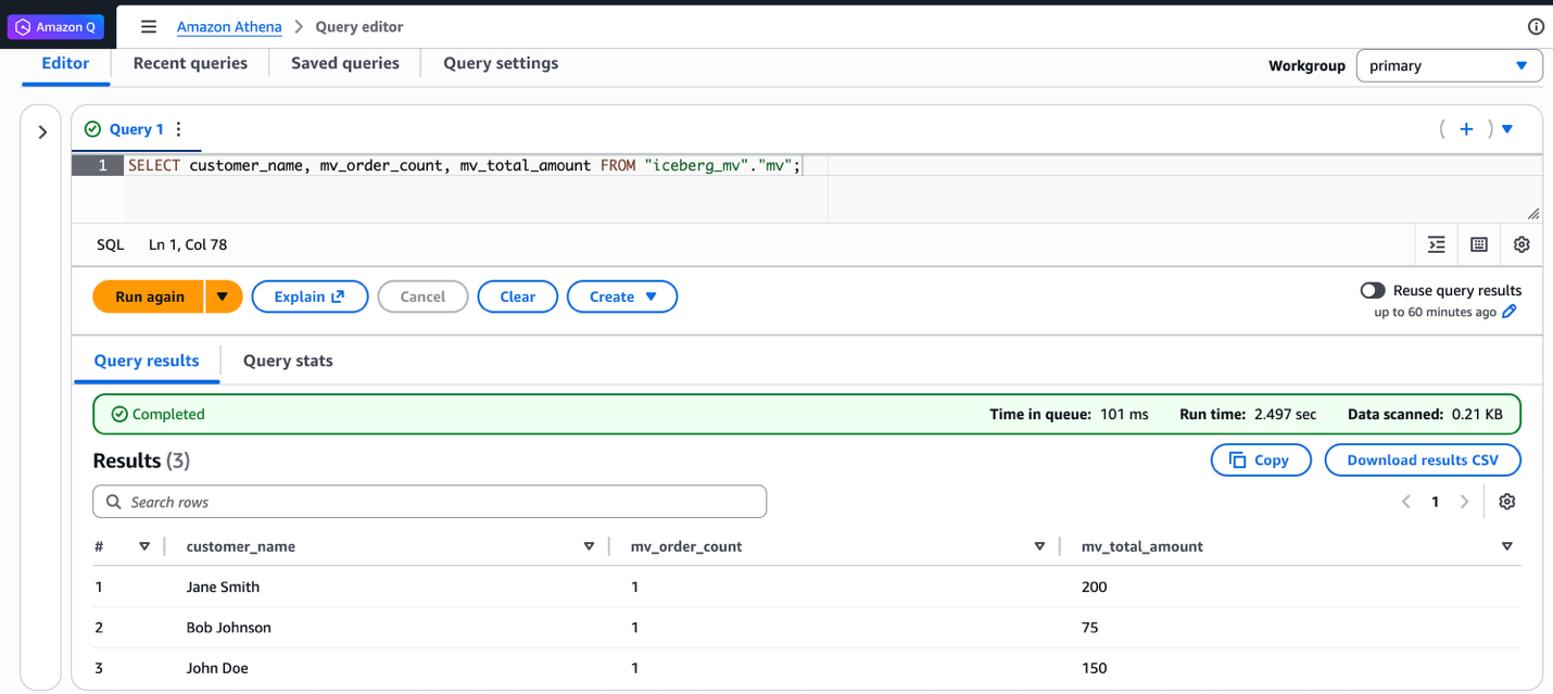
Additionally, you can query the same materialized view from Athena SQL. The following screenshot shows the same query run on Athena and the resulting output.

Refresh a materialized view

You can refresh materialized views using two refresh types: full refresh or incremental refresh. Full refresh re-computes the entire materialized view from all base table data. Incremental refresh processes only the changes since the last refresh. Full refresh is ideal when you need consistency or after significant data changes. Incremental refresh is preferred when you need immediate updates. The following examples show both refresh types.

To use full refresh, complete the following steps:

  1. Insert three new records into the base table to simulate new data arriving:
    INSERT INTO base_tbl VALUES 
    (4, 'Jane Smith', 350, DATE('2025-11-29')), 
    (5, 'Bob Johnson', 100, DATE('2025-11-30')), 
    (6, 'Kwaku Mensah', 40, DATE('2025-12-01'));

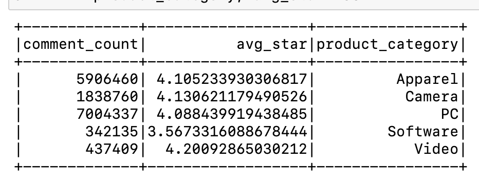
  2. Query the materialized view to verify it still shows the old aggregated values:
    SELECT * FROM mv;
    
    -- Result
    Jane Smith    1    200
    Bob Johnson    1    75
    John Doe    1    150

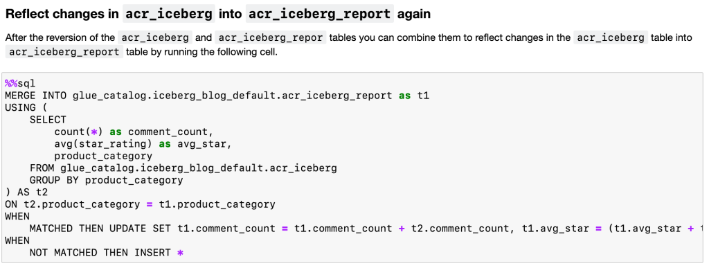
  3. Run a full refresh of the materialized view using the following command:
    REFRESH MATERIALIZED VIEW mv FULL;

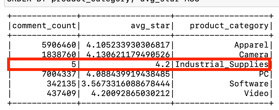
  4. Query the materialized view again to verify the aggregated values now include the new records:
    SELECT * FROM mv;
    
    -- Result
    Jane Smith    2    550 // Updated
    Bob Johnson    2    175  // Updated
    John Doe    1    150
    Kwaku Mensah    1    40 // Added

To use incremental refresh, complete the following steps:

  1. Enable incremental refresh by setting the Spark configuration properties:
    SET spark.sql.optimizer.incrementalMVRefresh.enabled=true;

  2. Insert two additional records into the base table:
    INSERT INTO base_tbl VALUES 
    (7, 'Jane Smith', 120, DATE('2025-11-28')), 
    (8, 'Kwaku Mensah', 90, DATE('2025-12-02'));

  3. Run an incremental refresh using the REFRESH command without the FULL clause. To verify if incremental refresh is enabled, refer to Appendix 2 at the end of this post.
    REFRESH MATERIALIZED VIEW mv;

  4. Query the materialized view to confirm the incremental changes are reflected in the aggregated results:
    SELECT * FROM mv;
    
    --Result
    Jane Smith    3    670    3    3 // Updated
    Bob Johnson    2    175    2    2 
    John Doe    1    150    1    1
    Kwaku Mensah    2    130    2    2 // Updated

In addition to using Spark SQL, you can also trigger manual refreshes through AWS Glue APIs when you need updates outside your scheduled intervals. Run the following AWS CLI command:

$ aws glue start-materialized-view-refresh-task-run \
    --catalog-id <ACCOUNT_ID> \
    --database-name <DATABASE_NAME> \
    --table-name <MV_TABLE_NAME>

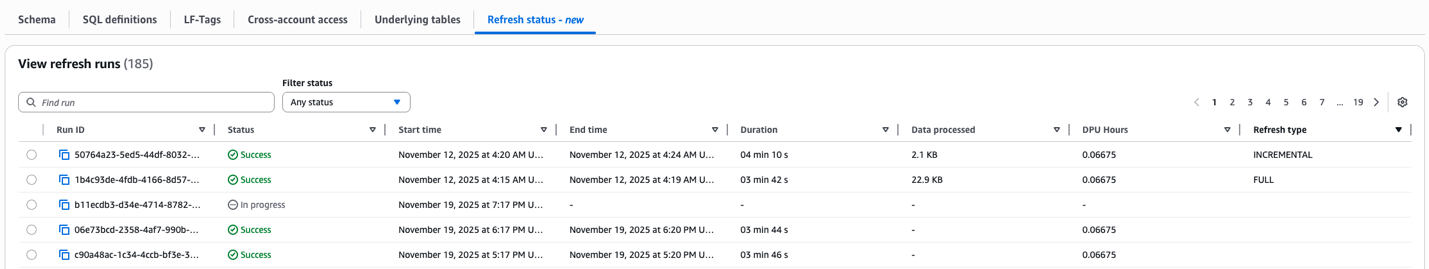
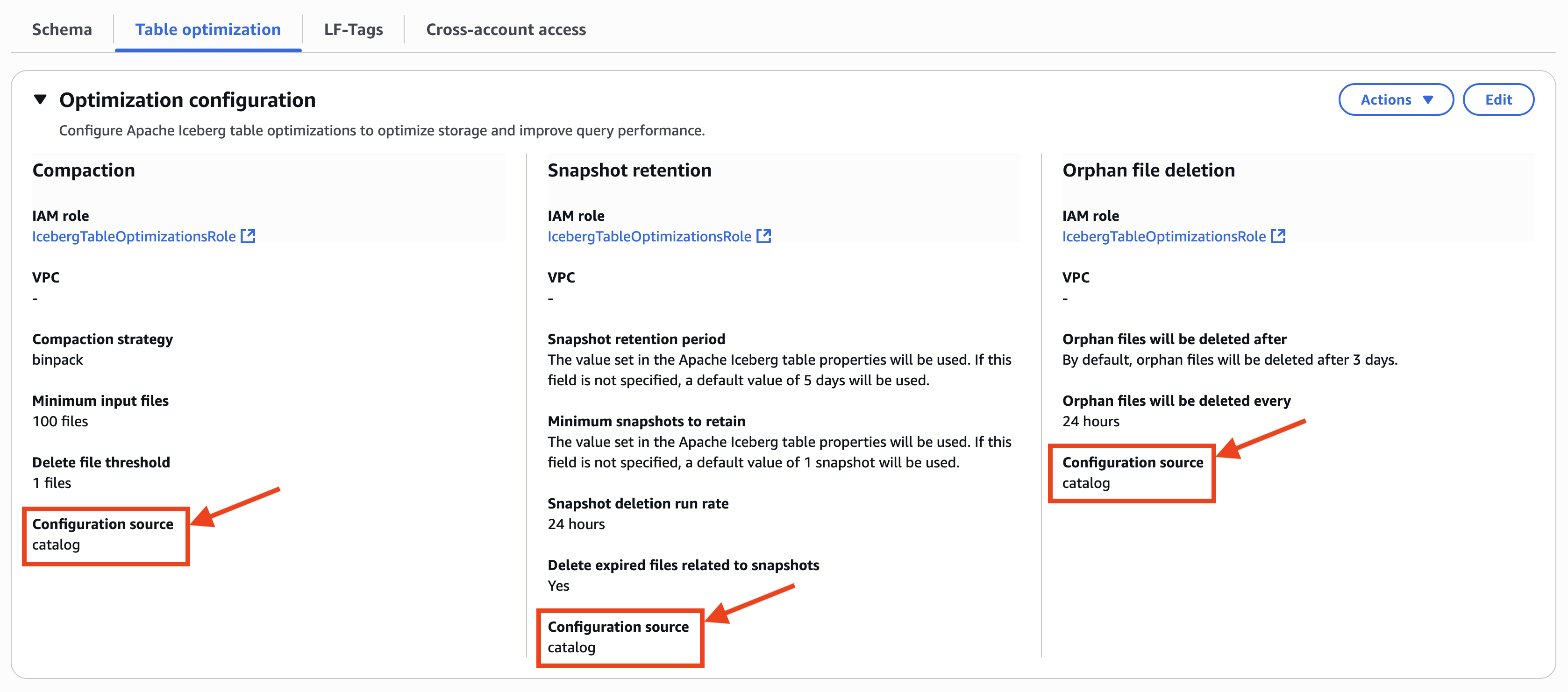
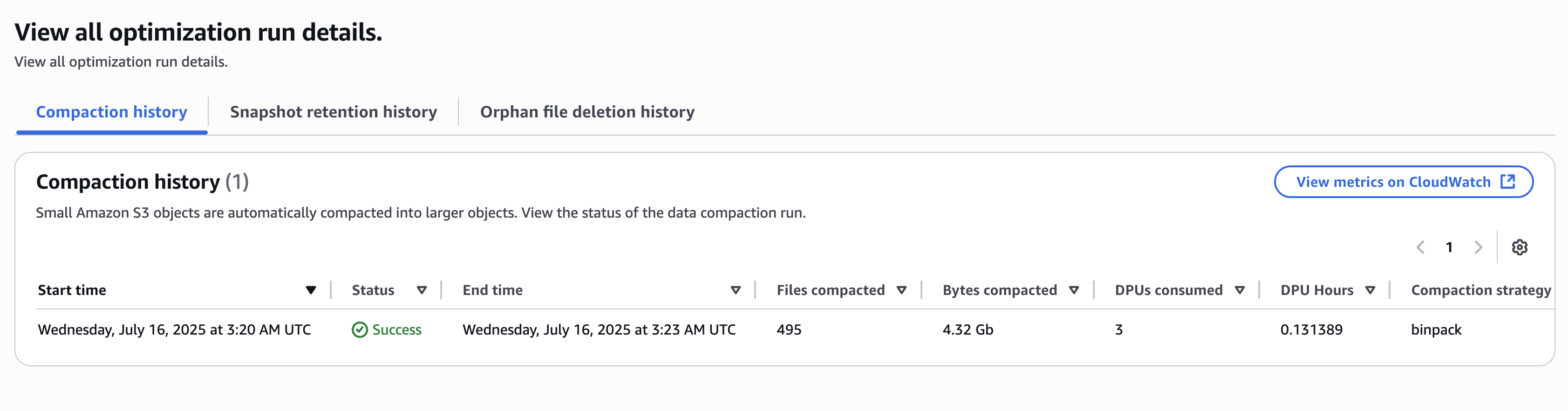
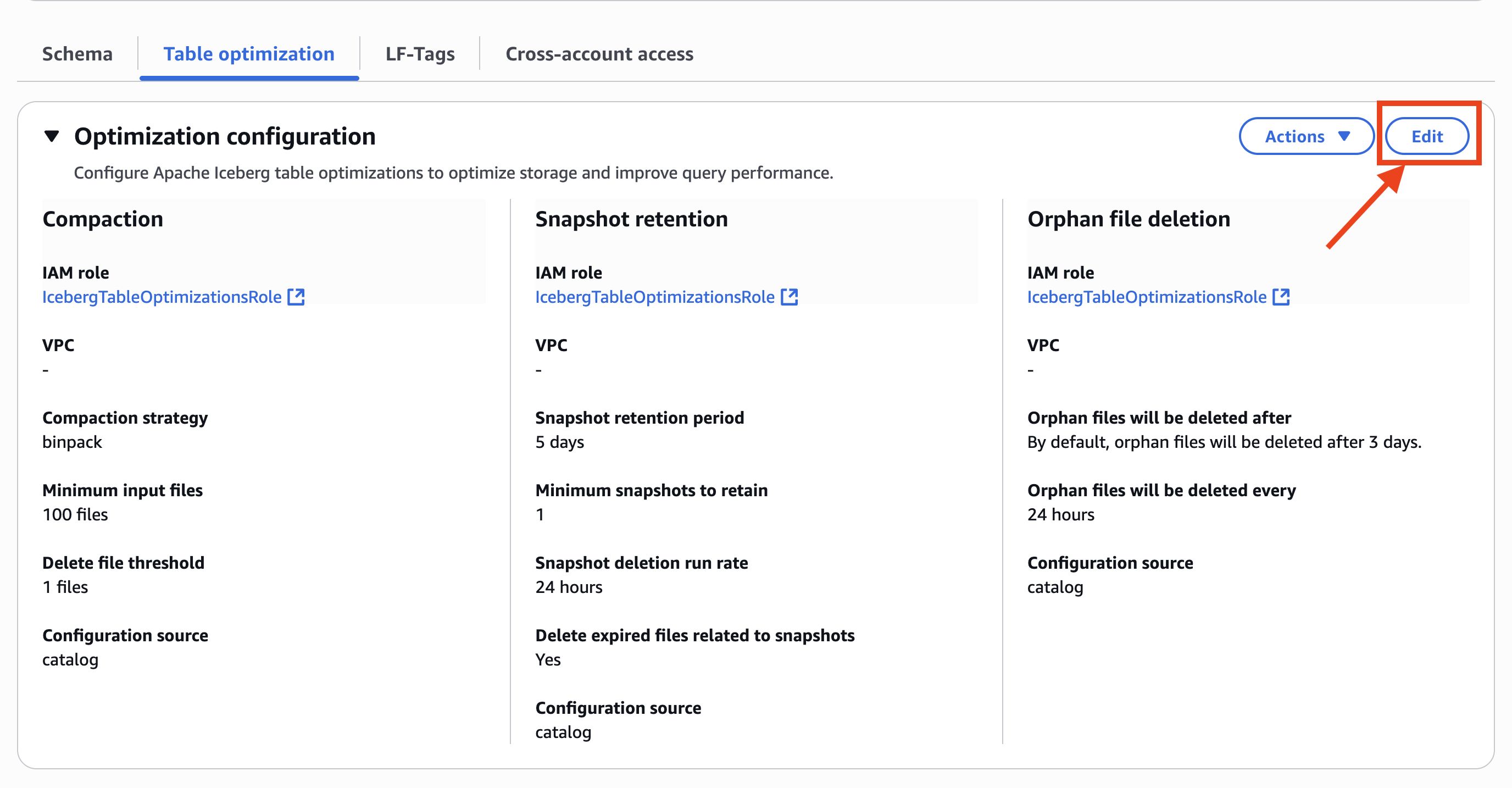
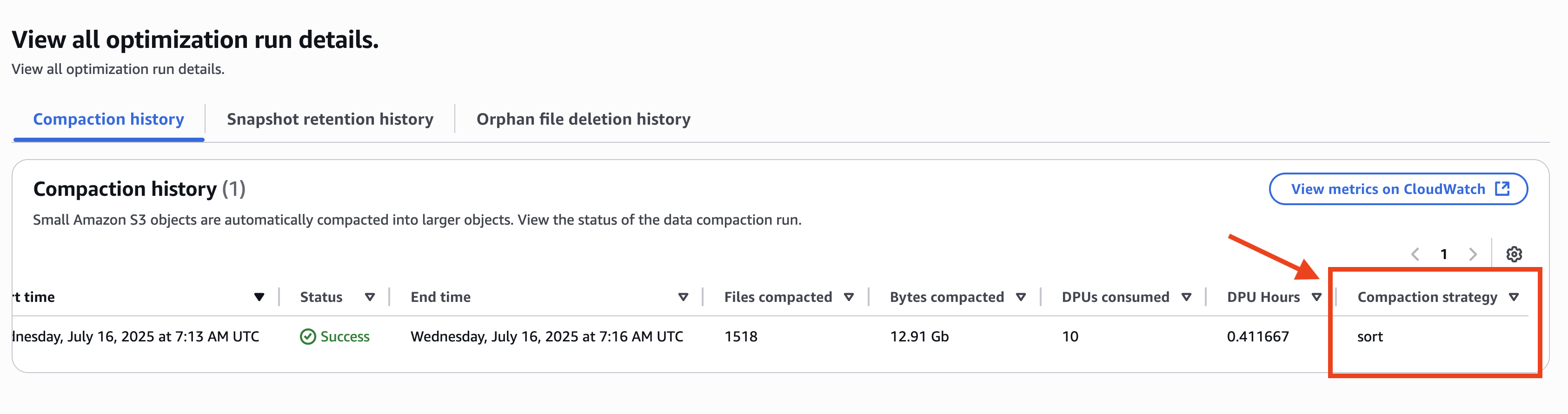
The AWS Lake Formation console displays refresh history for API-triggered updates. Open your materialized view to see the refresh type (INCREMENTAL or FULL), start and end time, status and so on:

You have learned how to use Iceberg materialized views to make your efficient data processing and queries. You created a materialized view using Spark on Amazon EMR, queried it from both Amazon EMR and Athena, and used two refresh mechanisms: full refresh and incremental refresh. Iceberg materialized views help you transform and optimize your data pipelines effortlessly.

Considerations

There are important aspects to consider for optimal usage of the capability:

  • We introduced new SQL syntax to manage materialized views in the AWS optimized Spark runtime engine only. These new SQL commands are available in Spark version 3.5.6 and above across Athena, Amazon EMR, and AWS Glue. Open source Spark is not supported.
  • Materialized views are eventually consistent with base tables. When source tables change, the materialized views are updated through background refresh processes as defined by users in the refresh schedule at creation. During the refresh window, queries directly accessing materialized views might see outdated data. However, customers who need immediate access to the most up-to-date datasets can run a manual refresh with a simple REFRESH MATERIALIZED VIEW SQL command.

Clean up

To avoid incurring future charges, clean up the resources you created during this walkthrough:

  1. Run the following commands to delete a materialized view and tables:
    DROP TABLE mv PURGE;
    -- Or, DROP MATERIALIZED VIEW mv;
    
    DROP TABLE base_tbl PURGE;
    -- If necessary, delete the database by DROP DATABASE iceberg_mv;

  2. For Amazon EMR, terminate the Amazon EMR cluster.
  3. For AWS Glue, delete the AWS Glue job.

Conclusion

This post demonstrated how Iceberg materialized views facilitate efficient data lake operations on AWS. The new materialized view capability simplifies data pipelines and improves query performance by storing pre-computed results that are automatically updated as base tables change. You can create materialized views using familiar SQL syntax, using both full and incremental refresh mechanisms to maintain data consistency. This solution alleviates the need for complex pipeline maintenance while providing seamless integration with AWS services like Athena, Amazon EMR, and AWS Glue. The automatic query rewrite functionality further optimizes performance by intelligently utilizing materialized views when applicable, making it a powerful tool for organizations looking to streamline their data transformation workflows and accelerate query performance.

Appendix 1: Spark configuration to use Amazon S3 Tables storing Apache Iceberg materialized views

As mentioned earlier in this post, materialized views are stored as Iceberg tables in Amazon S3 Tables buckets within your account. When you want to use Amazon S3 Tables as the storage location for your materialized views instead of a general Amazon S3 bucket, you must configure Spark with the Amazon S3 Tables catalog.

The difference from the standard AWS Glue Data Catalog configuration shown in the prerequisites section is the glue.id parameter format. For Amazon S3 Tables, use the format <account-id>:s3tablescatalog/<s3-tables-bucket-name> instead of just the account ID:

spark-sql \
  --conf spark.sql.extensions=org.apache.iceberg.spark.extensions.IcebergSparkSessionExtensions \
  --conf spark.sql.catalog.s3t_catalog=org.apache.iceberg.spark.SparkCatalog \
  --conf spark.sql.catalog.s3t_catalog.type=glue \
  --conf spark.sql.catalog.s3t_catalog.warehouse="s3://amzn-s3-demo-bucket/warehouse" \
  --conf spark.sql.catalog.s3t_catalog.glue.region="us-east-1" \
  --conf spark.sql.catalog.s3t_catalog.glue.id="123456789012:s3tablescatalog/amzn-s3-demo-table-bucket" \
  --conf spark.sql.catalog.s3t_catalog.glue.account-id=123456789012 \
  --conf spark.sql.catalog.s3t_catalog.client.region="us-east-1" \
  --conf spark.sql.catalog.s3t_catalog.glue.lakeformation-enabled=true \
  --conf spark.sql.optimizer.answerQueriesWithMVs.enabled=true \
  --conf spark.sql.defaultCatalog=s3t_catalog

After you configure Spark with these settings, you can create and manage materialized views using the same SQL commands shown in this post, and the materialized views are stored in your Amazon S3 Tables bucket.

Appendix 2: Verify refreshing a materialized view with Spark SQL

Run SHOW TBLPROPERTIES in Spark SQL to check which refresh method was used:

+-------------------------------+----------------------------------------------------------------------------------------------------------------------------------+
|key                            |value                                                                                                                             |
+-------------------------------+----------------------------------------------------------------------------------------------------------------------------------+
|IMV_ansiEnabled                |false                                                                                                                             |
|IMV_catalogInfo                |[{"catalogId":"123456789012","catalogName":"glue_catalog"}]                                                                       |
|IMV_mvCatalogID                |123456789012                                                                                                                      |
|IMV_mvNamespace                |iceberg_mv                                                                                                                        |
|IMV_region                     |us-east-1                                                                                                                         |
|IMV_sparkVersion               |3.5.6-amzn-1                                                                                                                      |
|current-snapshot-id            |5750703934418352571                                                                                                               |
|format                         |iceberg/parquet                                                                                                                   |
|format-version                 |2                                                                                                                                 |
|isMaterializedView             |true                                                                                                                              |
|lastRefreshType                |INCREMENTAL                                                                                                                       |
|subObjects                     |[{"Version":"4887707562550190856","DatabaseName":"iceberg_mv","Region":"us-east-1","CatalogId":"123456789012","Name":"base_tbl"}] |
|tableVersionToken              |*********(redacted)                                                                                                               |
|viewOriginalText               |SELECT\ncustomer_name, \nCOUNT(*) as mv_order_count, \nSUM(amount) as mv_total_amount \nFROM base_tbl\nGROUP BY customer_name     |
|viewVersionId                  |5750703934418352571                                                                                                               |
|viewVersionToken               |*********(redacted)                                                                                                               |
|write.parquet.compression-codec|zstd                                                                                                                              |
+-------------------------------+----------------------------------------------------------------------------------------------------------------------------------+

About the authors

Tomohiro Tanaka

Tomohiro Tanaka

Tomohiro is a Senior Cloud Support Engineer at AWS. He’s passionate about helping customers use Apache Iceberg for their data lakes on AWS. In his free time, he enjoys a coffee break with his colleagues and making coffee at home.

Leon Lin

Leon Lin

Leon is a Software Development Engineer at AWS, where he focuses on Apache Iceberg and Apache Spark development within the Open Data Analytics Engines team. He is also an active contributor to the open source Apache Iceberg project.

Noritaka Sekiyama

Noritaka Sekiyama

Noritaka is a Principal Big Data Architect with AWS Analytics services. He’s responsible for building software artifacts to help customers. In his spare time, he enjoys cycling on his road bike.

Mahesh Mishra

Mahesh Mishra

Mahesh is a Principal Product Manager with the AWS Analytics team. He works with many of AWS largest customers on emerging technology needs, and leads several data and analytics initiatives within AWS, including strong support for transactional data lakes.

Layth Yassin

Layth Yassin

Layth is a Software Development Engineer on the AWS Glue team. He’s passionate about tackling challenging problems at a large scale, and building products that push the limits of the field. Outside of work, he enjoys playing/watching basketball, and spending time with friends and family.

The Amazon SageMaker lakehouse architecture now automates optimization configuration of Apache Iceberg tables on Amazon S3

Post Syndicated from Tomohiro Tanaka original https://aws.amazon.com/blogs/big-data/the-amazon-sagemaker-lakehouse-architecture-now-automates-optimization-configuration-of-apache-iceberg-tables-on-amazon-s3/

As organizations increasingly adopt Apache Iceberg tables for their data lake architectures on Amazon Web Services (AWS), maintaining these tables becomes crucial for long-term success. Without proper maintenance, Iceberg tables can face several challenges: degraded query performance, unnecessary retention of old data that should be removed, and a decline in storage cost efficiency. These issues can significantly impact the effectiveness and economics of your data lake. Regular table maintenance operations help ensure your Iceberg tables remain high performing, compliant with data retention policies, and cost-effective for production workloads. To help you manage your Iceberg tables at scale, AWS Glue automated those Iceberg table maintenance operations: compaction with sort and z-order and snapshots expiration and orphan data management. After the launch of the feature, many customers have enabled automated table optimization through AWS Glue Data Catalog to reduce operational burden.

The Amazon SageMaker lakehouse architecture now automates optimization of Iceberg tables stored in Amazon S3 with catalog-level configuration, optimizing storage in your Iceberg tables and improving query performance. Previously, optimizing Iceberg tables in AWS Glue Data Catalog required updating configurations for each table individually. Now, you can enable automatic optimization for new Iceberg tables with one-time Data Catalog configuration. Once enabled, for any new table or updated table, Data Catalog continuously optimizes tables by compacting small files, removing snapshots, and unreferenced files that are no longer needed.

This post demonstrates an end-to-end flow to enable catalog level table optimization setting.

Prerequisites

The following prerequisites are required to use the new catalog-level table optimizations:

Enable table optimizations at the catalog level

The data lake administrator can enable the catalog-level table optimization on the AWS Lake Formation console. Complete the following steps:

  1. On the AWS Lake Formation console, choose Catalogs in the navigation pane.
  2. Select the catalog to be enabled with catalog-level table optimizations.
  3. Choose Table optimizations tab, and choose Edit in Table optimizations, as shown in the following screenshot.

setup-catalog-level-optimizations

  1. In Optimization options, select Compaction, Snapshot retention, and Orphan file deletion, as shown in the following screenshot.

enable-optimizations

  1. Select an IAM role. Refer to Table optimization prerequisites for permissions.
  2. Choose Grant required permissions.
  3. Choose I acknowledge that expired data will be deleted as part of the optimizers.

After you enable the table optimizations at the catalog level, the configuration is displayed on the AWS Lake Formation console, as shown in the following screenshot.

optimizations-configuration

When you select an Iceberg table registered in the catalog, you can confirm that the table optimizations configuration is inherited from the table view because Configuration source shows catalog, as shown in the following screenshot.

catalog-level-optimizations

The table optimizations history is displayed on the table view. The following result shows one of the compaction runs by the table optimizations.

binpack-compaction-result

The catalog-level table optimizations for all databases and Iceberg tables are now enabled.

Customize setting of table optimizations at both the catalog and table-level

Although the catalog-level optimization applies common settings across all databases and Iceberg tables in your catalog, you might want to apply different strategies for specific Iceberg tables. You can use AWS Glue Data Catalog to enable both catalog-level and table-level optimizations based on specific table characteristics and access patterns. For example, in addition to configuring the catalog-level compaction with the bin-pack strategy for general-purpose Iceberg tables, you can apply the sort strategy at the table-level to tables with frequent range queries on timestamp columns.

This section shows configuring catalog-level and table-specific optimizations through a practical scenario. Imagine a real-time analytics table with frequent write operations that generates more orphan files due to constant metadata updates. Users also run selective queries filtering specific columns, which makes sort-order strategy preferable. Complete the following steps:

  1. Select another Iceberg table in the same catalog as before to configure the table-level optimizations on the AWS Lake Formation console. At this point, the catalog-level table optimizations are configured for this table.
  2. Choose Edit in Optimization configuration, as shown in the following screenshot.

new-optimizations-configuration

  1. In Optimization options, choose Compaction, Snapshot retention, and Orphan file deletion.
  2. In Optimization configuration, choose Customize settings.
  3. Select the same IAM role.
  4. In Compaction configuration, select Sort, as shown in the following screenshot. Also configure 80 files to Minimum input files, which is a threshold of the number of files to trigger the compaction. To configure Sort, a sort order needs to be defined in your Iceberg table. You can define the sort order with Spark SQL such as ALTER TABLE db.tbl WRITE ORDERED BY <columns>.

sort-config

  1. In Snapshot retention configuration and Snapshot deletion run rate, select Specify a custom value in hours. Then, configure 12 hours to the interval between two deletion job runs, as shown in the following screenshot.

snapshot-retention

  1. In Orphan file deletion configuration, configure 1 day to Files under the provided Table Location with a creation time older than this number of days will be deleted if they are no longer referenced by the Apache Iceberg Table metadata.

orphan-deletion

  1. Choose Grant required permissions.
  2. Choose I acknowledge that expired data will be deleted as part of the optimizers.
  3. Choose Save.
  4. The Table optimization tab on the AWS Lake Formation console displays the custom setting of table optimizers. In Compaction, Compaction strategy is configured to sort and Minimum input files is also configured to 80 files. In Snapshot retention, Snapshot deletion run rate is configured to 12 hours. In Orphan file deletion, Orphan files will be deleted after is configured to 1 days, as shown in the following screenshot.

new-table-level-optimizations

The compaction history shows sort as its table-level compaction strategy even if the strategy in the catalog-level is configured to binpack, as shown in the following screenshot.

sort-compaction-result

In this scenario, the table-specific optimizations are configured along with the catalog-level optimizations. Combining the table and catalog-level optimizations means you can more flexibly manage your Iceberg table data deletions and compactions.

Conclusion

In this post, we demonstrated how to enable and manage using Amazon SageMaker lakehouse architecture with AWS Glue Data Catalog’s catalog-level table optimization feature for Iceberg tables. This enhancement significantly simplifies the management of Iceberg tables because you can enable automated maintenance operations across all tables with a single setting. Instead of configuring optimization settings for individual tables, you can now maintain your entire data lake more efficiently, reducing operational overhead while ensuring consistent optimization policies. We recommend enabling catalog-level table optimization to help you maintain a well-organized, high-performing, and cost-effective data lake while freeing up your teams to focus on deriving value from your data.

Try out this feature for your own use case and share your feedback and questions in the comments. To learn more about AWS Glue Data Catalog table optimizer, visit Optimizing Iceberg tables.

Acknowledgment: A special thanks to everyone who contributed to the development and launch of catalog level optimization: Siddharth Padmanabhan Ramanarayanan, Dhrithi Chidananda, Noella Jiang, Sangeet Lohariwala, Shyam Rathi, Anuj Jigneshkumar Vakil, and Jeremy Song.


About the authors

Tomohiro Tanaka is a Senior Cloud Support Engineer at Amazon Web Services (AWS). He’s passionate about helping customers use Apache Iceberg for their data lakes on AWS. In his free time, he enjoys a coffee break with his colleagues and making coffee at home.

Noritaka Sekiyama is a Principal Big Data Architect with AWS Analytics services. He’s responsible for building software artifacts to help customers. In his spare time, he enjoys cycling on his road bike.

Sandeep Adwankar is a Senior Product Manager at Amazon Web Services (AWS). Based in the California Bay Area, he works with customers around the globe to translate business and technical requirements into products customers can use to improve how they manage, secure, and access data.

Siddharth Padmanabhan Ramanarayanan is a Senior Software Engineer on the AWS Glue and AWS Lake Formation team, where he focuses on building scalable distributed systems for data analytics workloads. He is passionate about helping customers optimize their cloud infrastructure for performance and cost efficiency.

Build Write-Audit-Publish pattern with Apache Iceberg branching and AWS Glue Data Quality

Post Syndicated from Tomohiro Tanaka original https://aws.amazon.com/blogs/big-data/build-write-audit-publish-pattern-with-apache-iceberg-branching-and-aws-glue-data-quality/

Given the importance of data in the world today, organizations face the dual challenges of managing large-scale, continuously incoming data while vetting its quality and reliability. The importance of publishing only high-quality data can’t be overstated—it’s the foundation for accurate analytics, reliable machine learning (ML) models, and sound decision-making. Equally crucial is the ability to segregate and audit problematic data, not just for maintaining data integrity, but also for regulatory compliance, error analysis, and potential data recovery.

AWS Glue is a serverless data integration service that you can use to effectively monitor and manage data quality through AWS Glue Data Quality. Today, many customers build data quality validation pipelines using its Data Quality Definition Language (DQDL) because with static rules, dynamic rules, and anomaly detection capability, it’s fairly straightforward.

Apache Iceberg is an open table format that brings atomicity, consistency, isolation, and durability (ACID) transactions to data lakes, streamlining data management. One of its key features is the ability to manage data using branches. Each branch has its own lifecycle, allowing for flexible and efficient data management strategies.

This post explores robust strategies for maintaining data quality when ingesting data into Apache Iceberg tables using AWS Glue Data Quality and Iceberg branches. We discuss two common strategies to verify the quality of published data. We dive deep into the Write-Audit-Publish (WAP) pattern, demonstrating how it works with Apache Iceberg.

Strategy for managing data quality

When it comes to vetting data quality in streaming environments, two prominent strategies emerge: the dead-letter queue (DLQ) approach and the WAP pattern. Each strategy offers unique advantages and considerations.

  • The DLQ approach – Segregate problematic entries from high-quality data so that only clean data makes it into your primary dataset.
  • The WAP pattern – Using branches, segregate problematic entries from high-quality data so that only clean data is published in the main branch.

The DLQ approach

The DLQ strategy focuses on efficiently segregating high-quality data from problematic entries so that only clean data makes it into your primary dataset. Here’s how it works:

  1. As data streams in, it passes through a validation process
  2. Valid data is written directly to the table referred by downstream users
  3. Invalid or problematic data is redirected to a separate DLQ for later analysis and potential recovery

The following screenshot shows this flow.

bdb4341_0_1_dlq

Here are its advantages:

  • Simplicity – The DLQ approach is straightforward to implement, especially when there is only one writer
  • Low latency – Valid data is instantly available in the main branch for downstream consumers
  • Separate processing for invalid data – You can have dedicated jobs to process the DLQ for auditing and recovery purposes.

The DLQ strategy can present significant challenges in complex data environments. With multiple concurrent writers to the same Iceberg table, maintaining consistent DLQ implementation becomes difficult. This issue is compounded when different engines (for example, Spark, Trino, or Python) are used for writes because the DLQ logic may vary between them, making system maintenance more complex. Additionally, storing invalid data separately can lead to management overhead.

Additionally, for low-latency requirements, the processing validation step may introduce additional delays. This creates a challenge in balancing data quality with speed of delivery.

To solve those challenges in a reasonable way, we introduce the WAP pattern in the next section.

The WAP pattern

The WAP pattern implements a three-stage process:

  1. Write – Data is initially written to a staging branch
  2. Audit – Quality checks are performed on the staging branch
  3. Publish – Validated data is merged into the main branch for consumption

The following screenshot shows this flow.

bdb4341_0_2_wap

Here are its advantages:

  • Flexible data latency management – In the WAP pattern, the raw data is ingested to the staging branch without data validation, and then the high-quality data is ingested to the main branch with data validation. With this characteristic, there’s flexibility to achieve urgent, low-latency data handling on the staging branch and achieve high-quality data handling on the main branch.
  • Unified data quality management – The WAP pattern separates the audit and publish logic from the writer applications. It provides a unified approach to quality management, even with multiple writers or varying data sources. The audit phase can be customized and evolved without affecting the write or publish stages.

The primary challenge of the WAP pattern is the increased latency it introduces. The multistep process inevitably delays data availability for downstream consumers, which may be problematic for near real-time use cases. Furthermore, implementing this pattern requires more sophisticated orchestration compared to the DLQ approach, potentially increasing development time and complexity.

How the WAP pattern works with Iceberg

The following sections explore how the WAP pattern works with Iceberg.

Iceberg’s branching feature

Iceberg offers a branching feature for data lifecycle management, which is particularly useful for efficiently implementing the WAP pattern. The metadata of an Iceberg table stores a history of snapshots. These snapshots, created for each change to the table, are fundamental to concurrent access control and table versioning. Branches are independent histories of snapshots branched from another branch, and each branch can be referred to and updated separately.

When a table is created, it starts with only a main branch, and all transactions are initially written to it. You can create additional branches, such as an audit branch, and configure engines to write to them. Changes on one branch can be fast-forwarded to another branch using Spark’s fast_forward procedure, as shown in the following screenshot.

bdb4341_0_3_iceberg-branch

How to manage Iceberg branches

In this section, we cover the essential operations for managing Iceberg branches using SparkSQL. We’ll demonstrate how to use the branches, specifically, to create a new branch, write to and read from a specific branch, and set a default branch for a Spark session. These operations form the foundation for implementing the WAP pattern with Iceberg.

To create a branch, run the following SparkSQL query:

ALTER TABLE glue_catalog.db.tbl CREATE BRANCH audit

To specify a branch to be updated, use the glue_catalog.<database_name>.<table_name>.branch_<branch_name> syntax:

INSERT INTO glue_catalog.db.tbl.branch_audit VALUES (1, 'a'), (2, 'b');

To specify a branch to be queried, use the glue_catalog.<database_name>.<table_name>.branch_<branch_name> syntax:

SELECT * FROM glue_catalog.db.tbl.branch_audit;

To specify a branch for the entire Spark session scope, set the branch name to the Spark parameter spark.wap.branch. After this parameter is set, all queries will refer to the specified branch without explicit expression:

SET spark.wap.branch = audit

-- audit branch will be updated
INSERT INTO glue_catalog.db.tbl VALUES (3, 'c');

How to implement the WAP pattern with Iceberg branches

Using Iceberg’s branching feature, we can efficiently implement the WAP pattern with a single Iceberg table. Additionally, Iceberg characteristics such as ACID transactions and schema evolution are useful for handling multiple concurrent writers and varying data.

  1. Write – The data ingestion process switches branch from main and it commits updates to the audit branch, instead of the main branch. At this point, these updates aren’t accessible to downstream users who can only access the main branch.
  2. Audit – The audit process runs data quality checks on the data in the audit branch. It specifies which data is clean and ready to be provided.
  3. Publish – The audit process publishes validated data to the main branch with the Iceberg fast_forward procedure, making it available for downstream users.

This flow is shown in the following screenshot.

bdb4341_0_4_wap-w-iceberg-branch

By implementing the WAP pattern with Iceberg, we can obtain several advantages:

  • Simplicity – Iceberg branches can express multiple states of a table, such as audit and main, within one table. We can have unified data management even when handling multiple data contexts separately and uniformly.
  • Handling concurrent writers – Iceberg tables are ACID compliant, so consistent reads and writes are guaranteed even when multiple reader and writer processes run concurrently.
  • Schema evolution – If there are issues with the data being ingested, its schema may differ from the table definition. Spark supports dynamic schema merging for Iceberg tables. Iceberg tables can flexibly evolve their schema to write data with inconsistent schemas. By configuring the following parameters, when schema changes occur, new columns from the source are added to the target table with NULL values for existing rows. Columns present only in the target have their values set to NULL for new insertions or left unchanged during updates.
SET `spark.sql.iceberg.check-ordering` = false

ALTER TABLE glue_catalog.db.tbl SET TBLPROPERTIES (
    'write.spark.accept-any-schema'='true'
)
df.writeTo("glue_catalog.db.tbl").option("merge-schema","true").append()

As an intermediate wrap-up, the WAP pattern offers a robust approach to managing the balance between data quality and latency. With Iceberg branches, we can implement WAP pattern simply on single Iceberg table with handling concurrent writers and schema evolution.

Example use case

Suppose that a home monitoring system tracks room temperature and humidity. The system captures and sends the data to an Iceberg based data lake built on top of Amazon Simple Storage Service (Amazon S3). The data is visualized using matplotlib for interactive data analysis. For the system, issues such as device malfunctions or network problems can lead to partial or erroneous data being written, resulting in incorrect insights. In many cases, these issues are only detected after the data is sent to the data lake. Additionally, the correctness of such data is generally complicated.

To address these issues, the WAP pattern using Iceberg branches is applied for the system in this post. Through this approach, the incoming room data to the data lake is evaluated for quality before being visualized, and you make sure that only qualified room data is used for further data analysis. With the WAP pattern using the branches, you can achieve effective data management and promote data quality in downstream processes. The solution is demonstrated using AWS Glue Studio notebook, which is a managed Jupyter Notebook for interacting with Apache Spark.

Prerequisites

The following prerequisites are necessary for this use case:

Set up resources with AWS CloudFormation

First, you use a provided AWS CloudFormation template to set up resources to build Iceberg environments. The template creates the following resources:

  • An S3 bucket for metadata and data files of an Iceberg table
  • A database for the Iceberg table in AWS Glue Data Catalog
  • An AWS Identity and Access Management (IAM) role for an AWS Glue job

Complete the following steps to deploy the resources.

  1. Choose Launch stack.

Launch Button

  1. For the Parameters, IcebergDatabaseName is set by default. You can also change the default value. Then, choose Next.
  2. Choose Next.
  3. Choose I acknowledge that AWS CloudFormation might create IAM resources with custom names.
  4. Choose Submit.
  5. After the stack creation is complete, check the Outputs The resource values are used in the following sections.

Next, configure the Iceberg JAR files to the session to use the Iceberg branch feature. Complete the following steps:

  1. Select the following JAR files from the Iceberg releases page and download these JAR files on your local machine:
    1. 1.6.1 Spark 3.3_with Scala 2.12 runtime Jar
    2. 1.6.1 aws-bundle Jar
  2. Open the Amazon S3 console and select the S3 bucket you created through the CloudFormation stack. The S3 bucket name can be found on the CloudFormation Outputs tab.
  3. Choose Create folder and create the jars path in the S3 bucket.
  4. Upload the two downloaded JAR files to s3://<IcebergS3Bucket>/jars/ from the S3 console.

Upload a Jupyter Notebook on AWS Glue Studio

After launching the CloudFormation stack, you create an AWS Glue Studio notebook to use Iceberg with AWS Glue. Complete the following steps.

  1. Download wap.ipynb.
  2. Open AWS Glue Studio console.
  3. Under Create job, select Notebook.
  4. Select Upload Notebook, choose Choose file, and upload the notebook you downloaded.
  5. Select the IAM role name, such as IcebergWAPGlueJobRole, that you created through the CloudFormation stack. Then, choose Create notebook.
  6. For Job name at the left top of the page, enter iceberg_wap.
  7. Choose Save.

Configure Iceberg branches

Start by creating an Iceberg table that contains a room temperature and humidity dataset. After creating the Iceberg table, create branches that are used for performing the WAP practice. Complete the following steps:

  1. On the Jupyter Notebook that you created in Upload a Jupyter Notebook on AWS Glue Studio, run the following cell to use Iceberg with Glue. %additional_python_modules pandas==2.2 is used to visualize the temperature and humidity data in the notebook with pandas. Before running the cell, replace <IcebergS3Bucket> with the S3 bucket name where you uploaded the Iceberg JAR files.

bdb4341_1_session-config

  1. Initialize the SparkSession by running the following cell. The first three settings, starting with spark.sql, are required to use Iceberg with Glue. The default catalog name is set to glue_catalog using spark.sql.defaultCatalog. The configuration spark.sql.execution.arrow.pyspark.enabled is set to true and is used for data visualization with pandas.

bdb4341_2_sparksession-init

  1. After the session is created (the notification Session <Session Id> has been created. will be displayed in the notebook), run the following commands to copy the temperature and humidity dataset to the S3 bucket you created through the CloudFormation stack. Before running the cell, replace <IcebergS3Bucket> with the name of the S3 bucket for Iceberg, which you can find on the CloudFormation Outputs tab.
!aws s3 cp s3://aws-blogs-artifacts-public/artifacts/BDB-4341/data/part-00000-fa08487a-43c2-4398-bae9-9cb912f8843c-c000.snappy.parquet s3://<IcebergS3Bucket>/src-data/current/ 
!aws s3 cp s3://aws-blogs-artifacts-public/artifacts/BDB-4341/data/new-part-00000-e8a06ab0-f33d-4b3b-bd0a-f04d366f067e-c000.snappy.parquet s3://<IcebergS3Bucket>/src-data/new/
  1. Configure the data source bucket name and path (DATA_SRC), Iceberg data warehouse path (ICEBERG_LOC), and database and table names for an Iceberg table (DB_TBL). Replace <IcebergS3Bucket> with the S3 bucket from the CloudFormation Outputs tab.
  2. Read the dataset and create the Iceberg table with the dataset using the Create Table As Select (CTAS) query.

bdb4341_3_ctas

  1. Run the following code to display the temperature and humidity data for each room in the Iceberg table. Pandas and matplotlib are used to visualize the data for each room. The data from 10:05 to 10:30 is displayed in the notebook, as shown in the following screenshot, with each room showing approximately 25°C for temperature (displayed as the blue line) and 52% for humidity (displayed as the orange line).
import matplotlib.pyplot as plt
import pandas as pd

CONF = [
    {'room_type': 'myroom', 'cols':['current_temperature', 'current_humidity']},
    {'room_type': 'living', 'cols':['current_temperature', 'current_humidity']},
    {'room_type': 'kitchen', 'cols':['current_temperature', 'current_humidity']}
]

fig, axes = plt.subplots(nrows=3, ncols=1, sharex=True, sharey=True)
for ax, conf in zip(axes.ravel(), CONF):
    df_room = spark.sql(f"""
        SELECT current_time, current_temperature, current_humidity, room_type
        FROM {DB_TBL} WHERE room_type = '{conf['room_type']}'
        ORDER BY current_time ASC
        """)
    pdf = df_room.toPandas()
    pdf.set_index(pdf['current_time'], inplace=True)
    plt.xlabel('time')
    plt.ylabel('temperature/humidity')
    plt.ylim(10, 60)
    plt.yticks([tick for tick in range(10, 60, 10)])
    pdf[conf['cols']].plot.line(ax=ax, grid=True, figsize=(8, 6), title=conf['room_type'], legend=False, marker=".", markersize=2, linewidth=0)

plt.legend(['temperature', 'humidity'], loc='center', bbox_to_anchor=(0, 1, 1, 5.5), ncol=2)

%matplot plt

bdb4341_4_vis-1

  1. You create Iceberg branches by running the following queries before writing data into the Iceberg table. You can create an Iceberg branch by the ALTER TABLE db.table CREATE BRANCH <branch_name> query.
ALTER TABLE iceberg_wap_db.room_data CREATE BRANCH stg
ALTER TABLE iceberg_wap_db.room_data CREATE BRANCH audit

Now, you’re ready to build the WAP pattern with Iceberg.

Build WAP pattern with Iceberg

Use the Iceberg branches created earlier to implement the WAP pattern. You start writing the newly incoming temperature and humidity data including erroneous values to the stg branch in the Iceberg table.

Write phase: Write incoming data into the Iceberg stg branch

To write the incoming data into the stg branch in the Iceberg table, complete the following steps:

  1. Run the following cell and write the data into Iceberg table.

bdb4341_5_write

  1. After the records are written, run the following code to visualize the current temperature and humidity data in the stg On the following screenshot, notice that new data was added after 10:30. The output shows incorrect readings, such as around 100°C for temperature between 10:35 and 10:52 in the living room.
fig, axes = plt.subplots(nrows=3, ncols=1, sharex=True, sharey=True)
for ax, conf in zip(axes.ravel(), CONF):
    df_room_stg = spark.sql(f"""
        SELECT current_time, current_temperature, current_humidity, room_type
        FROM {DB_TBL}.branch_stg WHERE room_type = '{conf['room_type']}'
        ORDER BY current_time ASC
        """)
    pdf = df_room_stg.toPandas()
    pdf.set_index(pdf['current_time'], inplace=True)
    plt.xlabel('time')
    plt.ylabel('temperature/humidity')
    plt.ylim(10, 110)
    plt.yticks([tick for tick in range(10, 110, 30)])
    pdf[conf['cols']].plot.line(ax=ax, grid=True, figsize=(8, 6), title=conf['room_type'], legend=False, marker=".", markersize=2, linewidth=0)

plt.legend(['temperature', 'humidity'], loc='center', bbox_to_anchor=(0, 1, 1, 5.5), ncol=2)

%matplot plt

bdb4341_6_vis-2

The new temperature data including erroneous records was written to the stg branch. This data isn’t visible to the downstream side because it hasn’t been published to the main branch. Next, you evaluate the data quality in the stg branch.

Audit phase: Evaluate the data quality in the stg branch

In this phase, you evaluate the quality of the temperature and humidity data in the stg branch using AWS Glue Data Quality. Then, the data that doesn’t meet the criteria is filtered out based on the data quality rules, and the qualified data is used to update the latest snapshot in the audit branch. Start with the data quality evaluation:

  1. Run the following code to evaluate the current data quality using AWS Glue Data Quality. The evaluation rule is defined in DQ_RULESET, where the normal temperature range is set between −10 and 50°C based on the device specifications. Any values out of this range are considered erroneous in this scenario.
from awsglue.context import GlueContext
from awsglue.transforms import SelectFromCollection
from awsglue.dynamicframe import DynamicFrame
from awsgluedq.transforms import EvaluateDataQuality
DQ_RULESET = """Rules = [ ColumnValues "current_temperature" between -10 and 50 ]"""


dyf = DynamicFrame.fromDF(
    dataframe=spark.sql(f"SELECT * FROM {DB_TBL}.branch_stg"),
    glue_ctx=GlueContext(spark.sparkContext),
    name='dyf')

dyfc_eval_dq = EvaluateDataQuality().process_rows(
    frame=dyf,
    ruleset=DQ_RULESET,
    publishing_options={
        "dataQualityEvaluationContext": "dyfc_eval_dq",
        "enableDataQualityCloudWatchMetrics": False,
        "enableDataQualityResultsPublishing": False,
    },
    additional_options={"performanceTuning.caching": "CACHE_NOTHING"},
)

# Show DQ results
dyfc_rule_outcomes = SelectFromCollection.apply(
    dfc=dyfc_eval_dq,
    key="ruleOutcomes")
dyfc_rule_outcomes.toDF().select('Outcome', 'FailureReason').show(truncate=False)
  1. The output shows the result of the evaluation. It displays Failed because some temperature data, such as 105°C, is out of the normal temperature range of −10 to 50°C.
+-------+------------------------------------------------------+
|Outcome|FailureReason                                         |
+-------+------------------------------------------------------+
|Failed |Value: 105.0 does not meet the constraint requirement!|
+-------+------------------------------------------------------+
  1. After the evaluation, filter out the incorrect temperature data in the stg branch, then update the latest snapshot in the audit branch with the valid temperature data.

bdb4341_7_write-to-audit

Through the data quality evaluation, the audit branch in the Iceberg table now contains the valid data, which is ready for downstream use.

Publish phase: Publish the valid data to the downstream side

To publish the valid data in the audit branch to main, complete the following steps:

  1. Run the fast_forward Iceberg procedure to publish the valid data in the audit branch to the downstream side.

bdb4341_8_publish

  1. After the procedure is complete, review the published data by querying the main branch in the Iceberg table to simulate the query from the downstream side.
fig, axes = plt.subplots(nrows=3, ncols=1, sharex=True, sharey=True)
for ax, conf in zip(axes.ravel(), CONF):
    df_room_main = spark.sql(f"""
        SELECT current_time, current_temperature, current_humidity, room_type
        FROM {DB_TBL} WHERE room_type = '{conf['room_type']}'
        ORDER BY current_time ASC
        """)
    pdf = df_room_main.toPandas()
    pdf.set_index(pdf['current_time'], inplace=True)
    plt.xlabel('time')
    plt.ylabel('temperature/humidity')
    plt.ylim(10, 60)
    plt.yticks([tick for tick in range(10, 60, 10)])
    pdf[conf['cols']].plot.line(ax=ax, grid=True, figsize=(8, 6), title=conf['room_type'], legend=False, marker=".", markersize=2, linewidth=0)

plt.legend(['temperature', 'humidity'], loc='center', bbox_to_anchor=(0, 1, 1, 5.5), ncol=2)

%matplot plt

The query result shows only the valid temperature and humidity data that has passed the data quality evaluation.

bdb4341_9_vis-3

In this scenario, you successfully managed data quality by applying the WAP pattern with Iceberg branches. The room temperature and humidity data, including any erroneous records, was first written to the staging branch for quality evaluation. This approach prevented erroneous data from being visualized and leading to incorrect insights. After the data was validated by AWS Glue Data Quality, only valid data was published to the main branch and visualized in the notebook. Using the WAP pattern with Iceberg branches, you can make sure that only validated data is passed to the downstream side for further analysis.

Clean up resources

To clean up the resources, complete the following steps:

  1. On the Amazon S3 console, select the S3 bucket aws-glue-assets-<ACCOUNT_ID>-<REGION> where the Notebook file (iceberg_wap.ipynb) is stored. Delete the Notebook file located in the notebook path.
  2. Select the S3 bucket you created through the CloudFormation template. You can obtain the bucket name from IcebergS3Bucket key on the CloudFormation Outputs tab. After selecting the bucket, choose Empty to delete all objects.
  3. After you confirm the bucket is empty, delete the CloudFormation stack iceberg-wap-baseline-resources.

Conclusion

In this post, we explored common strategies for maintaining data quality when ingesting data into Apache Iceberg tables. The step-by-step instructions demonstrated how to implement the WAP pattern with Iceberg branches. For use cases requiring data quality validation, the WAP pattern provides the flexibility to manage data latency even with concurrent writer applications without impacting downstream applications.


About the Authors

Tomohiro Tanaka is a Senior Cloud Support Engineer at Amazon Web Services. He’s passionate about helping customers use Apache Iceberg for their data lakes on AWS. In his free time, he enjoys a coffee break with his colleagues and making coffee at home.

Sotaro Hikita is a Solutions Architect. He supports customers in a wide range of industries, especially the financial industry, to build better solutions. He is particularly passionate about big data technologies and open source software.

Noritaka Sekiyama is a Principal Big Data Architect on the AWS Glue team. He works based in Tokyo, Japan. He is responsible for building software artifacts to help customers. In his spare time, he enjoys cycling with his road bike.

Implement historical record lookup and Slowly Changing Dimensions Type-2 using Apache Iceberg

Post Syndicated from Tomohiro Tanaka original https://aws.amazon.com/blogs/big-data/implement-historical-record-lookup-and-slowly-changing-dimensions-type-2-using-apache-iceberg/

In today’s data-driven world, tracking and analyzing changes over time has become essential. As organizations process vast amounts of data, maintaining an accurate historical record is crucial. History management in data systems is fundamental for compliance, business intelligence, data quality, and time-based analysis. It enables organizations to maintain audit trails, perform trend analysis, identify data quality issues, and conduct point-in-time reporting. When combined with Change Data Capture (CDC), which identifies and captures database changes, history management becomes even more potent.

Common use cases for historical record management in CDC scenarios span various domains. In customer relationship management, it tracks changes in customer information over time. Financial systems use it for maintaining accurate transaction and balance histories. Inventory management benefits from historical data for analyzing sales patterns and optimizing stock levels. HR systems use it to track employee information changes. In fraud detection, historical data helps identify anomalous patterns in transactions or user behaviors.

This post will explore how to implement these functionalities using Apache Iceberg, focusing on Slowly Changing Dimensions (SCD) Type-2. This method creates new records for each data change while preserving old ones, thus maintaining a full history. By the end, you’ll understand how to use Apache Iceberg to manage historical records effectively on a typical CDC architecture.

Historical record lookup

How can we retrieve the history of given records? This is a fundamental question in data management, especially when dealing with systems that need to track changes over time. Let’s explore this concept with a practical example.

Consider a product (Heater) in an ecommerce database:

product_id product_name price
00001 Heater 250

Now, let’s say we update the price of this product from 250 to 500. After some time, we want to retrieve the price history of this heater. In a traditional database setup, this task could be challenging, especially if we haven’t explicitly designed our system to track historical changes.

This is where the concept of historical record lookup becomes crucial. We need a system that not only stores the current state of our data but also maintains a log of all changes made to each record over time. This allows us to answer questions like:

  • What was the price of the heater at a specific point in time?
  • How many times has the price changed, and when did these changes occur?
  • What was the price trend of the heater over the past year?

Implementing such a system can be complex, requiring careful consideration of data storage, retrieval mechanisms, and query optimization. This is where Apache Iceberg comes into play, offering a feature known as the change log view.

The change log view in Apache Iceberg provides a view of all changes made to a table over time, making it straightforward to query and analyze the history of any record. With change log view, we can easily track insertions, updates, and deletions, giving us a complete picture of how our data has evolved.

For our heater example, Iceberg’s change log view would allow us to effortlessly retrieve a timeline of all price changes, complete with timestamps and other relevant metadata, as shown in the following table.

product_id product_name price _change_type
00001 Heater 250 INSERT
00001 Heater 250 UPDATE_BEFORE
00001 Heater 500 UPDATE_AFTER

This capability not only simplifies historical analysis but also opens possibilities for advanced time-based analytics, auditing, and data governance.

Historical table lookup with SCD Type-2

SCD Type-2 is a key concept in data warehousing and historical data management and is particularly relevant to Change Data Capture (CDC) scenarios. SCD Type-2 creates new rows for changed data instead of overwriting existing records, allowing for comprehensive tracking of changes over time.

SCD Type-2 requires additional fields such as effective_start_date, effective_end_date, and current_flag to manage historical records. This approach has been widely used in data warehouses to track changes in various dimensions such as customer information, product details, and employee data. In the example of the previous section, here’s what the SCD Type-2 looks like assuming the update operation is performed on December 11, 2024.

product_id product_name price effective_start_date effective_end_date current_flag
00001 Heater 250 2024-12-10 2024-12-11 FALSE
00001 Heater 500 2024-12-11 NULL TRUE

SCD Type-2 is particularly valuable in CDC use cases, where capturing all data changes over time is crucial. It enables point-in-time analysis, provides detailed audit trails, aids in data quality management, and helps meet compliance requirements by preserving historical data.

In traditional implementations on data warehouses, SCD Type-2 requires its specific handling in all INSERT, UPDATE, and DELETE operations that affect those additional columns. For example, to update the price of the product, you need to run the following query.

UPDATE product SET effective_end_date = '2024-12-11', current_flag = false
WHERE product_id = '00001' AND current_flag = true;

INSERT INTO product (product_id, product_name, price, effective_start_date, effective_end_date, current_flag)
VALUES ('00001', 'Heater', 500, '2024-12-11', NULL, true);

For modern data lakes, we propose a new approach to implement SCD Type-2. With Iceberg, you can create a dedicated view of SCD Type-2 on top of the change log view, eliminating the need to implement specific handling to make changes on SCD Type-2 tables. With this approach, you can keep managing Iceberg tables without complexity considering SCD Type-2 specification. Anytime when you need SCD Type-2 snapshot of your Iceberg table, you can create the corresponding representation. This approach combines the power of Iceberg’s efficient data management with the historical tracking capabilities of SCD Type-2. By using the change log view, Iceberg can dynamically generate the SCD Type-2 structure without the overhead of maintaining additional tables or manually managing effective dates and flags.

This streamlined method not only makes the implementation of SCD Type-2 more straightforward, but also offers improved performance and scalability for handling large volumes of historical data in CDC scenarios. It represents a significant advancement in historical data management, merging traditional data warehousing concepts with modern big data capabilities.

As we delve deeper into Iceberg’s features, we’ll explore how this approach can be implemented, showcasing the efficiency and flexibility it brings to historical data analysis and CDC processes.

Prerequisites

The following prerequisites are required for the use cases:

Set up resources with AWS CloudFormation

Use a provided AWS CloudFormation template to set up resources to build Iceberg environments. The template creates the following resources:

Complete the following steps to deploy the resources.

  1. Choose Launch stack

Launch Button

  1. For the parameters, IcebergDatabaseName is set by default. You can change the default value. Then, choose Next.
  2. Choose Next
  3. Choose I acknowledge that AWS CloudFormation might create IAM resources with custom names.
  4. Choose Submit.
  5. After the stack creation is complete, check the Outputs tab and make a note of the resource values, which are used in the following sections.

Next, configure the Iceberg JAR files to the session to use the Iceberg change log view feature. Complete the following steps.

  1. Select the following JAR files from the Iceberg releases page and download these JAR files on your local machine:
    1. 1.6.1 Spark 3.3_with Scala 2.12 runtime Jar.
    2. 1.6.1 aws-bundle Jar.
  2. Open the Amazon S3 console and select the S3 bucket you created using the CloudFormation stack. The S3 bucket name can be found on the CloudFormation Outputs tab.
  3. Choose Create folder and create the jars path in the S3 bucket.
  4. Upload the two downloaded JAR files on s3://<IcebergS3Bucket>/jars/ from the S3 console.

Upload a Jupyter Notebook on AWS Glue Studio

After launching the CloudFormation stack, create an AWS Glue Studio notebook to use Iceberg with AWS Glue.

  1. Download history.ipynb.
  2. Open AWS Glue Studio console.
  3. Under Create job, select Notebook.
  4. Select Upload Notebook, choose Choose file and upload the Notebook you downloaded.
  5. Select the IAM role name such as IcebergHistoryGlueJobRole that you created using the CloudFormation template. Then, choose Create notebook.

1_upload-notebook

  1. For Job name at the left top of the page, enter iceberg_history.
  2. Choose Save.

Create an Iceberg table

To create an Iceberg table using a product dataset, complete the following steps.

  1. On the Jupyter Notebook that you created in Upload a Jupyter Notebook on AWS Glue Studio, run the following cell to use Iceberg with AWS Glue. Before running the cell, replace <IcebergS3Bucket> with the S3 bucket name where you uploaded the Iceberg JAR files.

2_session-config

  1. Initialize the SparkSession with Iceberg settings.

3_ss-init

  1. Configure database and table names for an Iceberg table (DB_TBL) and data warehouse path (ICEBERG_LOC). Replace <IcebergS3Bucket> with the S3 bucket from the CloudFormation Outputs tab.
  2. Run the following code to create the Iceberg table using the Spark DataFrame based on the product dataset.
from pyspark.sql import Row
import time
ut = time.time()
product = [
    {'product_id': '00001', 'product_name': 'Heater', 'price': 250, 'category': 'Electronics', 'updated_at': ut},
    {'product_id': '00002', 'product_name': 'Thermostat', 'price': 400, 'category': 'Electronics', 'updated_at': ut},
    {'product_id': '00003', 'product_name': 'Television', 'price': 600, 'category': 'Electronics', 'updated_at': ut},
    {'product_id': '00004', 'product_name': 'Blender', 'price': 100, 'category': 'Electronics', 'updated_at': ut},
    {'product_id': '00005', 'product_name': 'USB charger', 'price': 50, 'category': 'Electronics', 'updated_at': ut}
]
df_products = spark.createDataFrame(Row(**x) for x in product)
df_products.createOrReplaceTempView('tmp')

spark.sql(f"""
CREATE TABLE {DB_TBL} USING iceberg LOCATION '{ICEBERG_LOC}'
AS SELECT * FROM tmp
""")
  1. After creating the Iceberg table, run SELECT * FROM iceberg_history_db.products ORDER BY product_id to show the product data in the Iceberg table. Currently the following five products are stored in the Iceberg table.
+----------+------------+-----+-----------+--------------------+
|product_id|product_name|price|   category|          updated_at|
+----------+------------+-----+-----------+--------------------+
|     00001|      Heater|  250|Electronics|1.7297845122056053E9|
|     00002|  Thermostat|  400|Electronics|1.7297845122056053E9|
|     00003|  Television|  600|Electronics|1.7297845122056053E9|
|     00004|     Blender|  100|Electronics|1.7297845122056053E9|
|     00005| USB charger|   50|Electronics|1.7297845122056053E9|
+----------+------------+-----+-----------+--------------------+

Next, look up the historical changes for a product using Iceberg’s change log view feature.

Implement historical record lookup with Iceberg’s change log view

Suppose that there’s a source table whose table records are replicated to the Iceberg table through a Change Data Capture (CDC) process. When the records in the source table are updated, these changes are then mirrored in the Iceberg table. In this section, you look up the history of a given record for such a system to capture the history of product updates. For example, the following updates occur in the source table. Through the CDC process, these changes are applied to the Iceberg table.

  • Upsert (update and insert) the two records:
    • The price of Heater (product_id: 00001) is updated from 250 to 500.
    • A new product Chair (product_id: 00006) is added.
  • Television (product_id: 00003) is deleted.

To simulate the CDC workflow, you manually apply these changes to the Iceberg table in the notebook.

  1. Use the MERGE INTO query to upsert records. If an input record in the Spark DataFrame has the same product_id as an existing record, the existing record is updated. If no matching product_id is found, the input record is inserted into the Iceberg table.

4-merge-into

  1. Delete Television from the Iceberg table by running the DELETE query.
DELETE FROM iceberg_history_db.products WHERE product_id = '00003'
  1. Then, run SELECT * FROM iceberg_history_db.products ORDER BY product_id to show the product data in the Iceberg table. You can confirm that the price of Heater is updated to 500, Chair is added and Television is deleted.
+----------+------------+-----+-----------+--------------------+
|product_id|product_name|price|   category|          updated_at|
+----------+------------+-----+-----------+--------------------+
|     00001|      Heater|  500|Electronics|    1.729790106579E9|
|     00002|  Thermostat|  400|Electronics|1.7297845122056053E9|
|     00004|     Blender|  100|Electronics|1.7297845122056053E9|
|     00005| USB charger|   50|Electronics|1.7297845122056053E9|
|     00006|       Chair|   50|  Furniture|    1.729790106579E9|
+----------+------------+-----+-----------+--------------------+

For the Iceberg table, where changes from the source table are replicated, you can track the record changes using Iceberg’s change log view. To start, you first create a change log view from the Iceberg table.

  1. Run the create_changelog_view Iceberg procedure to create a change log view.

5-clv

  1. Run the following query to retrieve the historical changes for Heater.
SELECT product_id, product_name, price, category, updated_at, _change_type
FROM products_clv WHERE product_id = '00001'
ORDER BY _change_ordinal, _change_type DESC
  1. The query result shows the historical changes to Heater. You can confirm that the price of Heater was updated from 250 to 500 from the output.
+----------+------------+-----+-----------+--------------------+-------------+
|product_id|product_name|price|   category|          updated_at| _change_type|
+----------+------------+-----+-----------+--------------------+-------------+
|     00001|      Heater|  250|Electronics|1.7297902833360643E9|       INSERT|
|     00001|      Heater|  250|Electronics|1.7297902833360643E9|UPDATE_BEFORE|
|     00001|      Heater|  500|Electronics|1.7297903836233025E9| UPDATE_AFTER|
+----------+------------+-----+-----------+--------------------+-------------+

Using Iceberg’s change log view, you can obtain the history of a given record directly from the Iceberg table’s history, without needing to create a separate table for managing record history. Next, you implement Slowly Changing Dimension (SCD) Type-2 using the change log view.

Implement SCD Type-2 with Iceberg’s change log view

The SCD Type-2 based table retains the full history of record changes and it can be used in multiple cases such as historical tracking, point-in-time analysis, regulatory compliance, and so on. In this section, you implement SCD Type-2 using the change log view (products_clv) that was created in the previous section. The change log view has a schema that’s similar to the schema defined in the SCD Type-2 specifications. For this change log view, you add effective_start, effective_end, and is_current columns. To add these columns and then implement SCD Type-2, complete the following steps.

  1. Run the following query to implement SCD Type-2. In the WITH AS (...) section of the query, the change log view is merged with the Iceberg table snapshots using the snapshot_id key to include the commit time for each record change. You can obtain the table snapshots by querying for db.table.snapshots. The other part in the query identifies both current and non-current entries by comparing the commit times for each product. It then sets the effective time for each product, and marks whether a product is current or not based on the effective time and the change type from the change log view.
WITH clv_snapshots AS (
    SELECT
        clv.*,
        s.snapshot_id,
        s.committed_at,
        s.committed_at as effective_start
    FROM products_clv clv
    JOIN iceberg_history_db.products.snapshots s
    ON clv._commit_snapshot_id = s.snapshot_id
) 
SELECT
    product_id, 
    product_name, 
    price, 
    category, 
    updated_at,
    effective_start,
    CASE
        WHEN effective_start != l_part_committed_at 
            OR _change_type = 'UPDATE_BEFORE' THEN l_part_committed_at
        ELSE CAST(null as timestamp)
    END as effective_end,
    CASE
        WHEN effective_start != l_part_committed_at
            OR _change_type = 'UPDATE_BEFORE' 
            OR _change_type = 'DELETE' THEN CAST(false as boolean)
        ELSE CAST(true as boolean)
    END as is_current
FROM (SELECT *, MAX(committed_at) OVER (PARTITION BY product_id, updated_at) as l_part_committed_at FROM clv_snapshots)
WHERE _change_type != 'UPDATE_BEFORE'
ORDER BY product_id,  _change_ordinal
  1. The query result shows the SCD Type-2 based schema and records.

7-output

After the query result is displayed, this SCD Type-2 based table is stored as scdt2 to allow access for further analysis.

SCD Type-2 is useful for many use cases. To explore how this SCD Type-2 implementation can be used to track the history of table records, run the following example queries.

  1. Run the following query to retrieve deleted or updated records in a specific period. This query captures which records were changed during that timeframe, allowing you to audit changes for further use-cases such as trend analysis, regulatory compliance checks, and so on. Before running the query, replace <START_DATETIME> and <END_DATETIME> with specific time ranges such as 2024-10-24 17:18:00 and 2024-10-24 17:20:00.
SELECT product_id, product_name, price, category, updated_at, effective_start, effective_end, is_current 
FROM scdt2 WHERE product_id IN ( SELECT product_id FROM scdt2 
WHERE (_change_type = 'DELETE' or _change_type = 'UPDATE_AFTER') 
AND effective_start BETWEEN '<START_DATETIME>' AND '<END_DATETIME>') 
ORDER BY product_id, effective_start
  1. The query result shows the deleted and updated records in the specified period. You can confirm that the price of Heater was updated and Television was deleted from the table.
+----------+------------+-----+-----------+--------------------+--------------------+--------------------+----------+
|product_id|product_name|price|   category|          updated_at|     effective_start|       effective_end|is_current|
+----------+------------+-----+-----------+--------------------+--------------------+--------------------+----------+
|     00001|      Heater|  250|Electronics|1.7297902833360643E9|2024-10-24 17:18:...|2024-10-24 17:19:...|     false|
|     00001|      Heater|  500|Electronics|1.7297903836233025E9|2024-10-24 17:19:...|                null|      true|
|     00003|  Television|  600|Electronics|1.7297902833360643E9|2024-10-24 17:18:...|2024-10-24 17:19:...|     false|
|     00003|  Television|  600|Electronics|1.7297902833360643E9|2024-10-24 17:19:...|                null|     false|
+----------+------------+-----+-----------+--------------------+--------------------+--------------------+----------+
  1. As another example, run the following query to retrieve the latest records at a specific point in time from the SCD Type-2 table by filtering with is_current = true for current data reporting.
SELECT product_id, product_name, price, category, updated_at
FROM scdt2 WHERE is_current = true ORDER BY product_id
  1. The query result shows the current table records, reflecting the updated price of Heater, the deletion of Television, and the addition of Chair after the initial records.
+----------+------------+-----+-----------+--------------------+
|product_id|product_name|price|   category|          updated_at|
+----------+------------+-----+-----------+--------------------+
|     00001|      Heater|  500|Electronics|1.7297903836233025E9|
|     00002|  Thermostat|  400|Electronics|1.7297902833360643E9|
|     00004|     Blender|  100|Electronics|1.7297902833360643E9|
|     00005| USB charger|   50|Electronics|1.7297902833360643E9|
|     00006|       Chair|   50|  Furniture|1.7297903836233025E9|
+----------+------------+-----+-----------+--------------------+

You have now successfully implemented SCD Type-2 using the change log view. This SCD Type-2 implementation allows you to track the history of table records. For example, you can use it to search for deleted or updated products such as Heater and Chair in a specific period. Additionally, you can retrieve the current table records by querying the SCD Type-2 table with is_current = true. Using Iceberg’s change log view enables you to implement SCD Type-2 without making any changes to the Iceberg table itself. It also eliminates the need for creating or managing an additional table for SCD Type-2.

Clean up

To clean up the resources used in this post, complete the following steps:

  1. Open the Amazon S3 console
  2. Select the S3 bucket aws-glue-assets-<ACCOUNT_ID>-<REGION> where the Notebook file (iceberg_history.ipynb) is stored. Delete the Notebook file that’s in the notebook path.
  3. Select the S3 bucket you created using the CloudFormation template. You can obtain the bucket name from IcebergS3Bucket key on the CloudFormation Outputs tab. After selecting the bucket, choose Empty to delete all objects
  4. After you confirm the bucket is empty, delete the CloudFormation stack iceberg-history-baseline-resources.

Considerations

Here are important considerations:

Conclusion

In this post, we have explored how to look up the history of records and tables using Apache Iceberg. The instruction demonstrated how to use change log view to look up the history of the records, and also the history of the tables with SCD Type-2. With this method, you can manage the history of records and tables without extra effort.


About the Authors

Tomohiro Tanaka is a Senior Cloud Support Engineer at Amazon Web Services. He’s passionate about helping customers use Apache Iceberg for their data lakes on AWS. In his free time, he enjoys a coffee break with his colleagues and making coffee at home.

Noritaka Sekiyama is a Principal Big Data Architect on the AWS Glue team. He works based in Tokyo, Japan. He is responsible for building software artifacts to help customers. In his spare time, he enjoys cycling with his road bike.

Expand data access through Apache Iceberg using Delta Lake UniForm on AWS

Post Syndicated from Tomohiro Tanaka original https://aws.amazon.com/blogs/big-data/expand-data-access-through-apache-iceberg-using-delta-lake-uniform-on-aws/

The landscape of big data management has been transformed by the rising popularity of open table formats such as Apache Iceberg, Apache Hudi, and Linux Foundation Delta Lake. These formats, designed to address the limitations of traditional data storage systems, have become essential in modern data architectures. As organizations adopt various open table formats to suit their specific needs, the demand for interoperability between these formats has grown significantly. This interoperability is crucial for enabling seamless data access, reducing data silos, and fostering a more flexible and efficient data ecosystem.

Delta Lake UniForm is an open table format extension designed to provide a universal data representation that can be efficiently read by different processing engines. It aims to bridge the gap between various data formats and processing systems, offering a standardized approach to data storage and retrieval. With UniForm, you can read Delta Lake tables as Apache Iceberg tables. This expands data access to broader options of analytics engines.

This post explores how to start using Delta Lake UniForm on Amazon Web Services (AWS). You can learn how to query Delta Lake native tables through UniForm from different data warehouses or engines such as Amazon Redshift as an example of expanding data access to more engines.

How Delta Lake UniForm works

UniForm allows other table format clients such as Apache Iceberg to access Delta Lake tables. Under the hood, UniForm generates Iceberg metadata files (including metadata and manifest files) that are required for Iceberg clients to access the underlying data files in Delta Lake tables. Both Delta Lake and Iceberg metadata files reference the same data files. UniForm generates multiple table format metadata without duplicating the actual data files. When an Iceberg client reads a UniForm table, it first accesses the Iceberg metadata files for the UniForm table, which then allows the Iceberg client to read the underlying data files.

There are two options to use UniForm:

  • Create a new Delta Lake table with UniForm
  • Enable UniForm on your existing Delta Lake table

First, to create a new Delta Lake table enabling UniForm, you configure table properties for UniForm in a CREATE TABLE DDL query. The table properties are 'delta.universalFormat.enabledFormats'='iceberg' and 'delta.enableIcebergCompatV2'='true'. When these options are set to the CREATE TABLE query, Iceberg metadata files are generated along with Delta Lake metadata files. In addition to these options, Delta Lake table protocol versions that define supported features by the table such as delta.minReaderVersion and delta.minWriterVersion are required to be set to 2 and 7 or more respectively. For more information about the table protocol versions, refer to What is a table protocol specification? in Delta Lake public document. Appendix 1. Create a new Delta Lake table with UniForm shows an example query to create a new Delta Lake UniForm table.

You can also enable UniForm on an existing Delta Lake table. This option is suitable if you have Delta Lake tables in your environment. Enabling UniForm doesn’t affect your current operations on the Delta Lake tables. To enable UniForm on a Delta Lake table, run REORG TABLE db.existing_delta_lake_table APPLY (UPGRADE UNIFORM(ICEBERG_COMPAT_VERSION=2)). After running this query, Delta Lake automatically generates Iceberg metadata files for the Iceberg client. In the example in this post, you run this option and enable UniForm after you create a Delta Lake table.

For the information about enabling UniForm, refer to Enable Delta Lake UniForm in the Delta Lake public document. Note that the extra package (delta-iceberg) is required to create a UniForm table in AWS Glue Data Catalog. The extra package is also required to generate Iceberg metadata along with Delta Lake metadata for the UniForm table.

Example use case

A fictional company built a data lake with Delta Lake on Amazon Simple Storage Service (Amazon S3) that’s mainly used through Amazon Athena. According to its usage expansion, this company wants to expand data access to cloud-based data warehouses such as Amazon Redshift for flexible analytics use cases.

There are a few challenges to achieve this requirement. Delta Lake isn’t natively supported in Amazon Redshift. For those data warehouses, Delta Lake tables need to be converted to manifest tables, which requires additional operational overhead. You need to run the GENERATE command on Spark or use a crawler in AWS Glue to generate manifest tables, and you need to sync those manifest tables every time the Delta tables are updated.

Delta Lake UniForm can be a solution to meet this requirement. With Delta Lake UniForm, you can make the Delta Table compatible with the other open table formats such as Apache Iceberg, which is natively supported in Amazon Redshift. Users can query those Delta Lake tables as Iceberg tables through UniForm.

The following diagram describes the architectural overview to achieve that requirement.

bdb4538_solution-overview

In this tutorial, you create a Delta Lake table with a synthetic review dataset that includes different products and customer reviews and enable UniForm on that Delta Lake table to make it accessible from Amazon Redshift. Each component works as follows in this scenario:

  • Amazon EMR (Amazon EMR on EC2 cluster with Apache Spark): An Apache Spark application on an Amazon EMR cluster creates a Delta Lake table and enables UniForm on it. Only Delta Lake client can write to the Delta Lake UniForm table, making Amazon EMR act as a writer.
  • Amazon Redshift: Amazon Redshift uses Iceberg clients to read records from the Delta Lake UniForm table. It’s limited to reading records from the table and cannot write to it.
  • Amazon S3 and AWS Glue Data Catalog: These are used to manage the underlying files and the catalog of the Delta Lake UniForm table. The data and metadata files for the table are stored in an S3 bucket. The table is registered in AWS Glue Data Catalog.

Set up resources

In this section, you complete the following resource setup:

  1. Launch an AWS CloudFormation template to configure resources such as S3 buckets, an Amazon Virtual Private Cloud (Amazon VPC) and a subnet, a database for Delta Lake in Data Catalog, AWS Identity and Access Management (IAM) policy and role with required permissions for Amazon EMR Studio, and an EC2 instance profile for Amazon EMR on EC2 cluster
  2. Launch an Amazon EMR on EC2 cluster
  3. Create an Amazon EMR Studio Workspace
  4. Upload a Jupyter Notebook on Amazon EMR Studio Workspace
  5. Launch a CloudFormation template to configure Amazon Redshift Serverless and relevant subnets

Launch a CloudFormation template to configure basic resources

You use a provided CloudFormation template to set up resources to build Delta Lake UniForm environments. The template creates the following resources.

  • An S3 bucket to store the Delta Lake table data
  • An S3 bucket to store an Amazon EMR Studio Workspace metadata and configuration files
  • An IAM role for Amazon EMR Studio
  • An EC2 instance profile for Amazon EMR on EC2 cluster
  • VPC and subnet for an Amazon EMR on EC2 cluster
  • A database for a Delta Lake table in Data Catalog

Complete the following steps to deploy the resources.

  1. Choose Launch stack:

  1. For Stack name, enter delta-lake-uniform-on-aws. For the Parameters, DeltaDatabaseName, PublicSubnetForEMRonEC2, and VpcCIDRForEMRonEC2 are set by default. You can also change the default values. Then, choose Next.
  2. Choose Next.
  3. Choose I acknowledge that AWS CloudFormation might create IAM resources with custom names.
  4. Choose Submit.
  5. After the stack creation is complete, check the Outputs. The resource values are used in the following sections and in the Appendices.

Launch an Amazon EMR on EC2 cluster

Complete the following steps to create an Amazon EMR on EC2 cluster.

  1. Open the Amazon EMR on EC2 console.
  2. Choose Create cluster.
  3. Enter delta-lake-uniform-blog-post in Name and confirm choosing emr-7.3.0 as its release label.
  4. For Application bundle, select Spark 3.5.1Hadoop 3.3.6 and JupyterEnterpriseGateway 2.6.0.
  5. For AWS Glue Data Catalog settings, enable Use for Spark table metadata.
  6. For Networking, enter the values from the CloudFormation Outputs tab for VpcForEMR and PublicSubnetForEMR into Virtual private cloud (VPC) andSubnet respectively. For EC2 security groups, keep Create ElasticMapReduce-Primary for Primary node, and Create ElasticMapReduce-Core for Core and task nodes. The security groups for the Amazon EMR primary and core nodes are automatically created.
  7. For Cluster logs, enter s3://<DeltaLakeS3Bucket>/emr-cluster-logs as the Amazon S3 location. Replace <DeltaLakeS3Bucket> with the S3 bucket from the CloudFormation stack Outputs tab.
  8. For Software settings, select Load JSON from Amazon S3 and enter s3://aws-blogs-artifacts-public/artifacts/BDB-4538/config.json as the Amazon S3 location.
  9. For Amazon EMR service role in Identity and Access Management (IAM) roles section, choose Create a service role. Then, set default to Security Group. If there are existing security groups for Amazon EMR Primary and Core or Task nodes, set those security groups to Security Group.
  10. For EC2 instance profile for Amazon EMR, choose Choose an existing instance profile, and set EMRInstanceProfileRole to Instance profile.
  11. After reviewing the configuration, choose Create cluster.
  12. After the cluster status is Waiting on the Amazon EMR console, the cluster setup is complete (it approximately takes 10 minutes).

Create an Amazon EMR Studio Workspace

Complete the following steps to create an Amazon EMR Studio Workspace to use Delta Lake UniForm on Amazon EMR on EC2.

  1. Open Amazon EMR Studio console.
  2. Choose Create Studio.
  3. For Setup options, choose Custom.
  4. For Studio settings, enter delta-lake-uniform-studio as the Studio name.
  5. For S3 location for Workspace storage, choose Select existing location as a Workspace storage. The S3 location (s3://aws-emr-studio-<ACCOUNT_ID>-<REGION>-delta-lake-uniform-on-aws) can be obtained from EMRStudioS3Bucket on the CloudFormation Outputs tab. Then, choose EMRStudioRole as the IAM role (you can find the IAM Role name on the CloudFormation Outputs tab).
  6. For Workspace settings, enter delta-lake-workspace as the Workspace name.
  7. In Networking and security, choose the VPC ID and Subnet ID that you created in Launch an AWS CloudFormation template. You can obtain the VPC ID and Subnet ID from the VpcForEMR and PublicSubnetForEMR keys on the CloudFormation Outputs tab respectively.
  8. After reviewing the settings, choose Create Studio and launch Workspace.
  9. After creating the Studio Workspace is complete, you are redirected to Jupyter Notebook.

Upload Jupyter Notebook

Complete the following steps to configure a Jupyter Notebook to use Delta Lake UniForm with Amazon EMR.

  1. Download delta-lake-uniform-on-aws.ipynb.
  2. Choose the arrow icon at the top of the page and upload the Notebook you just downloaded.

  1. Choose and open the notebook (delta-lake-uniform-on-aws.ipynb) you uploaded in the left pane.
  2. After the notebook is opened, choose EMR Compute in the navigation pane.

  1. Attach the Amazon EMR on EC2 cluster you created in the previous section. Choose EMR on EC2 cluster and set the cluster you created previously to EMR on EC2 cluster, then choose Attach.
  2. After attaching the cluster is successful, Cluster is attached to the Workspace is displayed on the console.

Create a workgroup and a namespace for Amazon Redshift Serverless

For this step, you configure a workgroup and a namespace for Amazon Redshift Serverless to run queries on a Delta Lake UniForm table. You also configure two subnets in the same VPC created by the CloudFormation stack delta-lake-uniform-on-aws. To deploy the resources, complete the following steps:

  1. Choose Launch stack:

  1. For Stack name, enter redshift-serverless-for-delta-lake-uniform.
  2. For Parameters, enter the Availability Zone and an IP range for each subnet. The VPC ID is automatically retrieved from the CloudFormation stack you created in Launch an AWS CloudFormation template to configure basic resources. If you change the default subnet, note that at least one subnet needs to be the same subnet you created for the Amazon EMR on EC2 cluster (by default, the subnet for Amazon EMR on EC2 cluster is automatically retrieved during this CloudFormation stack creation). You can check the subnet for the cluster on the CloudFormation Outputs Then, choose Next.
  3. Choose Next again, and then choose Submit.
  4. After the stack creation is complete, check the CloudFormation Outputs Make a note of the two Subnet IDs on the Outputs tab to use later in Run queries from Amazon Redshift against the UniForm table.

Now you’re ready to use Delta Lake UniForm on Amazon EMR.

Enable Delta Lake UniForm

Start by creating a Delta Lake table that contains the customer review dataset. After creating the table, run REORG query to enable UniForm on the Delta Lake table.

Create a Delta Lake table

Complete the following steps to create a Delta Lake table based on a customer review dataset and review the table metadata.

  1. Return to the Jupyter Notebook connected to the Amazon EMR on EC2 cluster and run the following cell to add delta-iceberg.jar to use UniForm and configure the spark extension.

  1. Initialize the SparkSession. The following configuration is necessary to use Iceberg through UniForm. Before running the code, replace <DeltaLakeS3Bucket> with the name of the S3 bucket for Delta Lake, which you can find on the CloudFormation stack Outputs tab.

bdb4538-2_2-notebook

  1. Create a Spark DataFrame from customer reviews.

bdb4538-2_3-notebook_df

  1. Create a Delta Lake table with the customer reviews dataset. This step takes approximately 5 minutes.

bdb4538-2_4-notebook

  1. Run DESCRIBE EXTENDED {DB_TBL} in the next cell to review the table. The output includes the table schema, location, table properties, and so on.

bdb4538-2_5-notebook

The Delta Lake table creation is complete. Next, enable UniForm on this Delta Lake table.

Run REORG query to enable UniForm

To allow an Iceberg client to access the Delta Lake table you created, enable UniForm on the table. You can also create a new Delta Lake table with UniForm enabled. For more information, see Appendix 1 at the end of this post. To enable UniForm and review the table metadata, complete the following steps.

  1. Run the following query to enable UniForm on the Delta Lake table. To enable UniForm on an existing Delta Lake table, you run REORG query against the table.

bdb4539-3_1-uniform_reorg

  1. Run DESCRIBE EXTENDED {DB_TBL} in the next cell to review the table metadata and compare it from before and after enabling UniForm. The new properties, such as delta.enableIcebergCompatV2=true and delta.universalFormat.enabledFormats=iceberg, are added to the table properties.

bdb4538-3_2-uniform_metadata

  1. Run aws s3 ls s3://<DeltaLakeS3Bucket>/warehouse/ --recursive to confirm if the Iceberg table metadata is created. Replace <DeltaLakeS3Bucket> with the S3 bucket from the CloudFormation Outputs tab. The following screenshot shows the command output of table metadata and data files. You can confirm that Delta Lake UniForm generates both Iceberg metadata and Delta Lake metadata files as indicated by the red rectangles below.

bdb4538-3_3-uniform_metadata

  1. Before querying the Delta Lake UniForm table from an Iceberg client, run the following analytic query for the Delta Lake UniForm table from Amazon EMR on EC2 side, and review the reviews count by each product category.

bdb4538-3_4-uniform_query

  1. The query result shows the output of the reviews count by product_category:

Enabling UniForm on the Delta Lake table is complete, and now you can query the Delta Lake table from an Iceberg client. Next, you query the Delta Lake table as an Iceberg table from Amazon Redshift.

Run queries against the UniForm table from Amazon Redshift

In the previous section, you enabled UniForm on your existing Delta Lake table. This allows you to run queries on a Delta Lake table as if it were an Iceberg table from Amazon Redshift. In this section, you run an analytic query on the UniForm table using Amazon Redshift Serverless and add records with a new product category to the UniForm table through the Jupyter Notebook connected to the Amazon EMR on EC2 cluster. Then, you verify the added records with another analytic query from Amazon Redshift. You can confirm that Delta Lake UniForm enables Amazon Redshift to query the Delta Lake table through this section.

Query the UniForm table from Amazon Redshift Serverless

  1. Open Amazon Redshift Serverless console
  2. In Namespaces/Workgroups, select the delta-lake-uniform-namespace that you created using the CloudFormation stack.
  3. Choose Query data on the right top corner to open the Amazon Redshift query editor.
  4. After opening the editor, select the delta-lake-uniform-workgroup workgroup in the left pane.
  5. Choose Create connection.
  6. After you successfully create a connection, you can see the delta_uniform_db database and customer_review table you created in the left pane of the editor.
  7. Copy and paste the following analytic query to the editor and choose Run.
SELECT product_category, count(*) as count_by_product_category 
FROM "awsdatacatalog"."delta_uniform_db"."customer_reviews"
GROUP BY product_category ORDER BY count_by_product_category DESC
  1. The editor shows the same result of the review count by product_category as you obtained from Jupyter Notebook in Run REORG query to enable UniForm.

bdb4538-4_1-rs_result

Add new product category records into Delta Lake UniForm table from Amazon EMR

Go back to the Jupyter Notebook on Amazon EMR Workspace to add new records with a new product category (Books) into the Delta Lake UniForm table. After adding the records, query the UniForm table again from Amazon Redshift Serverless.

  1. On the Jupyter Notebook, go to Add new product category records into the UniForm table and run the following cell to load new records.

bdb4538-4_2-append_books

  1. Run the following cell and review the five records with Books as the product category. The following screenshot shows the output of this code.

bdb4538-4_3-append_listbooks

  1. Add the new reviews with Books product category. This takes around 2 minutes.

bdb4538-4_4-append_append

In the next section, you run a query on the UniForm table from Amazon Redshift Serverless to check if the new records with the Books product category have been added.

Review the added records in Delta Lake UniForm table from Amazon Redshift Serverless

To check if the result output includes the records of Books product category:

  1. On the query editor of Amazon Redshift, run the following query and check if the result output includes the records of Books product category.
SELECT product_category, count(*) as count_by_product_category 
FROM "awsdatacatalog"."delta_uniform_db"."customer_reviews"
GROUP BY product_category ORDER BY count_by_product_category DESC
  1. The following screenshot shows the output of the query you ran in the previous step. You can confirm the new product category Books has been added to the table from Amazon Redshift side.

bdb4538-4_5-rs-result
Now you can query from Amazon Redshift against the Delta Lake table by enabling Delta Lake UniForm.

Clean up resources

To clean up your resources, complete the following steps:

  1. In the Amazon EMR Workspaces console, choose Actions and then Delete to delete the workspace.
  2. Choose Delete to delete the Studio.
  3. In the Amazon EMR on EC2 console, choose Terminate to delete the Amazon EMR on EC2 cluster.
  4. In the Amazon S3 console, choose Empty to delete all objects in the following S3 buckets.
    1. The S3 bucket for Amazon EMR Studio such as aws-emr-studio-<ACCOUNT_ID>-<REGION>-delta-lake-uniform-on-aws. Replace <ACCOUNT_ID> and <REGION> with your account ID and the bucket’s region.
    2. The S3 bucket for Delta Lake tables such as delta-lake-uniform-on-aws-deltalakes3bucket-abcdefghijk.
  5. After you confirm the two buckets are empty, delete the CloudFormation stack redshift-serverless-for-delta-lake-uniform.
  6. After the first CloudFormation stack has been deleted, delete the CloudFormation stack delta-lake-uniform-on-aws.

Conclusion

Delta Lake UniForm on AWS represents an advancement in addressing the challenges of data interoperability and accessibility in modern big data architectures. By enabling Delta Lake tables to be read as Apache Iceberg tables, UniForm expands data access capabilities, allowing organizations to use a broader range of analytics engines and data warehouses such as Amazon Redshift.

The practical implications of this technology are substantial, offering new possibilities for data analysis and insights across diverse platforms. As organizations continue to navigate the complexities of big data, solutions like Delta Lake UniForm that promote interoperability and reduce data silos will become increasingly valuable.

By adopting these advanced open table formats and using cloud platforms such as AWS, organizations can build more robust and efficient data ecosystems. This approach not only enhances the value of existing data assets but also fosters a more agile and adaptable data strategy, ultimately driving innovation and improving decision-making processes in our data-driven world.

Appendix 1: Create a new Delta Lake table with UniForm

You can create a Delta Lake table with UniForm enabled using the following DDL.

CREATE TABLE IF NOT EXISTS delta_uniform_db.customer_reviews_create (
   marketplace string,
   customer_id string,
   review_id string,
   product_id string,
   product_title string,
   star_rating bigint,
   helpful_votes bigint,
   total_votes bigint,
   insight string,
   review_headline string,
   review_body string,
   review_date timestamp,
   review_year bigint,
   product_category string)
USING delta
TBLPROPERTIES ( 
   'delta.universalFormat.enabledFormats'='iceberg',
   'delta.enableIcebergCompatV2'='true',
   'delta.minReaderVersion'='2',
   'delta.minWriterVersion'='7')

Appendix 2: Run queries from Snowflake against the UniForm table

Delta Lake UniForm also allows you to run queries on a Delta Lake table from Snowflake. In this section, you run the same analytic query on the UniForm table using Snowflake as you previously did using Amazon Redshift Serverless in Run queries from Amazon Redshift against the UniForm table. Then you confirm that the query results from Snowflake match the results obtained from the Amazon Redshift Serverless query.

Configure IAM roles for Snowflake to access AWS Glue Data Catalog and Amazon S3

To query the Delta Lake UniForm table in Data Catalog from Snowflake, the following configurations are required.

  1. IAM roles: Create IAM roles for Snowflake to access Data Catalog and Amazon S3.
  2. Data Catalog integration with Snowflake: Snowflake provides two catalog options for Iceberg tables such as Using Snowflake as the Iceberg catalog and Using an external catalog such as Data Catalog. In this post, you choose AWS Glue Data Catalog as an external catalog. For information about the catalog options, refer to Iceberg catalog options in the Snowflake public documentation.
  3. An external volume creation for Amazon S3: To access the UniForm table from Snowflake, an external volume for Amazon S3 needs to be configured. With this configuration, Snowflake can connect the S3 bucket that you created for Iceberg tables. For information about the external volume, refer to Configure an external volume for Iceberg tables.

Create IAM roles for Snowflake to access AWS Glue Data Catalog and Amazon S3

Create the following two IAM roles for Snowflake to access AWS Glue Data Catalog and Amazon S3.

  • SnowflakeIcebergGlueCatalogRole: This IAM role is used for Snowflake to access the Delta Lake UniForm table in AWS Glue Data Catalog.
  • SnowflakeIcebergS3Role: This IAM role is used for Snowflake to access the table’s underlying data in the S3 bucket.

To configure the IAM roles, complete the following steps:

  1. Choose Launch stack:

  1. Enter snowflake-iceberg as the stack name and choose Next.
  2. Select I acknowledge that AWS CloudFormation might create IAM resources with custom names.
  3. Choose Submit.
  4. After the stack creation is complete, check the CloudFormation Outputs tab. Make a note of the names and ARNs of the two IAM roles, which are used in the following section.

Create an AWS Glue Data Catalog Integration

Create a catalog integration for AWS Glue Data Catalog. For more information about the catalog integration for AWS Glue Data Catalog, refer to Configure a catalog integration for AWS Glue in the Snowflake public documentation. To configure the catalog integration, complete the following steps:

  1. Access your Snowflake account and open an empty worksheet (query editor).
  2. Run the following query and create a catalog integration with AWS Glue Data Catalog. Replace <YOUR_ACCOUNT_ID> with the IAM role ARN from the snowflake-iceberg CloudFormation Ouputs tab, and replace <REGION> with the region of AWS Glue Data Catalog.
CREATE CATALOG INTEGRATION glue_catalog_integration
  CATALOG_SOURCE=GLUE
  CATALOG_NAMESPACE='delta_uniform_db'
  TABLE_FORMAT=ICEBERG
  GLUE_AWS_ROLE_ARN='arn:aws:iam::<YOUR_ACCOUNT_ID>:role/SnowflakeIcebergGlueCatalogRole'
  GLUE_CATALOG_ID='<YOUR_ACCOUNT_ID>'
  GLUE_REGION='<REGION>'
  ENABLED=TRUE;
  1. Retrieve GLUE_AWS_IAM_USER_ARN and GLUE_AWS_EXTERNAL_ID by using DESCRIBE CATALOG INTEGRATION glue_catalog_integration in the editor. The output is similar to the following:
+------------------------------------------------------------------------------------------------------------------------------+
| property                 | property_type | property_value                                                 | property_default |
|--------------------------+---------------+----------------------------------------------------------------+------------------|
| ENABLED                  | Boolean       | true                                                           | false            |
| CATALOG_SOURCE           | String        | GLUE                                                           |                  |
| CATALOG_NAMESPACE        | String        | delta_uniform_db                                               |                  |
| TABLE_FORMAT             | String        | ICEBERG                                                        |                  |
| REFRESH_INTERVAL_SECONDS | Integer       | 30                                                             | 30               |
| GLUE_AWS_ROLE_ARN        | String        | arn:aws:iam::123456789012:role/SnowflakeIcebergGlueCatalogRole |                  |
| GLUE_CATALOG_ID          | String        | 123456789012                                                   |                  |
| GLUE_REGION              | String        | us-east-1                                                      |                  |
| GLUE_AWS_IAM_USER_ARN    | String        | arn:aws:iam::123456789012:user/<ID>                            |                  |
| GLUE_AWS_EXTERNAL_ID     | String        | An external ID specified on the IAM Role trust relationships   |                  |
| COMMENT                  | String        |                                                                |                  |
+------------------------------------------------------------------------------------------------------------------------------+
  1. Update the IAM role you created using the CloudFormation stack to enable Snowflake to access AWS Glue Data Catalog using that IAM role. Open Trust Relationships of SnowflakeIcebergGlueCatalogRole on the IAM console, choose Edit and update the trust relationship using the following policy. Replace <GLUE_AWS_IAM_USER_ARN> and <GLUE_AWS_EXTERNAL_ID> with the names you obtained in the previous step.
{
   "Version": "2012-10-17",
   "Statement": [
	  {
		 "Sid": "",
		 "Effect": "Allow",
		 "Principal": {
			"AWS": "<GLUE_AWS_IAM_USER_ARN>"
		 },
		 "Action": "sts:AssumeRole",
		 "Condition": {
			"StringEquals": {
			   "sts:ExternalId": "<GLUE_AWS_EXTERNAL_ID>"
			}
		 }
	  }
   ]
}

You completed setting up the IAM role for Snowflake to access your Data Catalog resources. Next, configure the IAM role for Amazon S3 access.

Register Amazon S3 as an external volume

In this section, you configure an external volume for Amazon S3. Snowflake accesses the UniForm table data files in S3 through the external volume. For the configuration of an external volume for S3, refer to Configure an external volume for Amazon S3 in Snowflake public documentation. To configure the external volume, complete the following steps:

  1. In the query editor, run the following query to create an external volume for the Delta Lake S3 bucket. Replace <DeltaLakeS3Bucket> with the name of the S3 bucket that you created in Launch a CloudFormation template to configure basic resources from the CloudFormation Outputs tab. Replace <ACCOUNT_ID> with your AWS account ID.
CREATE OR REPLACE EXTERNAL VOLUME delta_lake_uniform_s3
   STORAGE_LOCATIONS =
	  (
		 (
			NAME = 'delta-lake-uniform-on-aws'
			STORAGE_PROVIDER = 'S3'
			STORAGE_BASE_URL = 's3://<DeltaLakeS3Bucket>'
			STORAGE_AWS_ROLE_ARN = 'arn:aws:iam::<ACCOUNT_ID>:role/SnowflakeIcebergS3Role'
		 )
	  );
  1. Retrieve STORAGE_AWS_IAM_USER_ARN and STORAGE_AWS_EXTERNAL_ID by running DESCRIBE EXTERNAL VOLUME delta_lake_uniform_s3 in the editor. The output is similar to the following:
+------------------------------------------------------------------------------------------------------------------------------------------------------------------------------------------------------------------+
| parent_property   | property           | property_type | property_value                                                                                                                       | property_default |
|-------------------+--------------------+---------------+--------------------------------------------------------------------------------------------------------------------------------------+------------------|
|                   | ALLOW_WRITES       | Boolean       | true                                                                                                                                 | true             |
| STORAGE_LOCATIONS | STORAGE_LOCATION_1 | String        | {"NAME":"uniform_s3_location","STORAGE_PROVIDER":"S3","STORAGE_BASE_URL":"s3://<DeltaLakeS3Bucket>","STORAGE_ALLOWED_LOCATIONS":["s3 |                  |
|                   |                    |               | ://<DeltaLakeS3Bucket>/*"],"STORAGE_REGION":"us-east-1","PRIVILEGES_VERIFIED":true,"STORAGE_AWS_ROLE_ARN":"arn:aws:iam::123456789012 |                  |
|                   |                    |               | :role/SnowflakeIcebergS3Role","STORAGE_AWS_IAM_USER_ARN":"arn:aws:iam::123456789012:user/<ID>","STORAGE_AWS_EXTERNAL_ID":"<External  |                  |
|                   |                    |               | ID>",... }                                                                                                                           |                  |
| STORAGE_LOCATIONS | ACTIVE             | String        | uniform_s3_location                                                                                                                  |                  |
+------------------------------------------------------------------------------------------------------------------------------------------------------------------------------------------------------------------+
  1. Update the IAM role you created using the CloudFormation template (in Create IAM roles for Snowflake to access AWS Glue Data Catalog and Amazon S3) to enable Snowflake to use this IAM role. Open Trust Relationships of SnowflakeIcebergS3Role on the IAM console, choose Edit, and update the trust relationship with the following policy. Replace <STORAGE_AWS_IAM_USER_ARN> and <STORAGE_AWS_EXTERNAL_ID> with the values from the previous step.
{
  "Version": "2012-10-17",
  "Statement": [
    {
      "Sid": "",
      "Effect": "Allow",
      "Principal": {
        "AWS": "<STORAGE_AWS_IAM_USER_ARN&>"
      },
      "Action": "sts:AssumeRole",
      "Condition": {
        "StringEquals": {
          "sts:ExternalId": "<STORAGE_AWS_EXTERNAL_ID>"
        }
      }
    }
  ]
}

The next step is to create an Iceberg table to run queries from Snowflake.

Create an Iceberg table in Snowflake

In this section, you create an Iceberg table in Snowflake. The table is an entry point for Snowflake to access the Delta Lake UniForm table in AWS Glue Data Catalog. To create the table, complete the following steps:

  1. (Optional) If you don’t have a database in Snowflake, run CREATE DATABASE <DATABASE_NAME>, replacing <DATABASE_NAME> with a unique database name for the Iceberg table.
  2. Run the following query in the Snowflake query editor. In this case, the database delta_uniform_snow_db is chosen for the table. Configure the following parameters:
    1. EXTERNAL_VOLUME: created by CREATE OR REPLACE EXTERNAL VOLUME query in the previous section, such as delta_lake_uniform_s3.
    2. CATALOG: created by the CREATE CATALOG INTEGRATION query in the previous section, such as glue_catalog_integration.
    3. CATALOG_TABLE_NAME: the name of Delta Lake UniForm table you created in Data Catalog such as customer_reviews.

The complete query is below:

CREATE OR REPLACE ICEBERG TABLE customer_reviews_snow
  EXTERNAL_VOLUME='delta_lake_uniform_s3'
  CATALOG='glue_catalog_integration'
  CATALOG_TABLE_NAME='customer_reviews';

After the table creation is complete, you’re ready to query the UniForm table in AWS Glue Data Catalog from Snowflake.

Query the UniForm table from Snowflake

In this step, you query the UniForm table from Snowflake. Paste and run the following analytic query in the Snowflake query editor.

SELECT product_category, count(*) as count_by_product_category 
FROM customer_reviews_snow 
GROUP BY product_category ORDER BY count_by_product_category DESC

The query result shows the same output as you saw in Review the added records in Delta Lake UniForm table from Amazon Redshift Serverless section.

+--------------------------------------------------+
| PRODUCT_CATEGORY     | COUNT_BY_PRODUCT_CATEGORY |
|----------------------+---------------------------|
| Office_Products      | 9673711                   |
| Books                | 9672664                   |
| Apparel              | 6448747                   |
| Computers            | 3224215                   |
| Beauty_Personal_Care | 3223599                   |
+--------------------------------------------------+

Now you can query from Snowflake against the Delta Lake table by enabling Delta Lake UniForm.


About the Authors

Tomohiro Tanaka is a Senior Cloud Support Engineer at Amazon Web Services. He’s passionate about helping customers use Apache Iceberg for their data lakes on AWS. In his free time, he enjoys a coffee break with his colleagues and making coffee at home.

Noritaka Sekiyama is a Principal Big Data Architect on the AWS Glue team. He works based in Tokyo, Japan. He is responsible for building software artifacts to help customers. In his spare time, he enjoys cycling with his road bike.

Use the AWS Glue connector to read and write Apache Iceberg tables with ACID transactions and perform time travel

Post Syndicated from Tomohiro Tanaka original https://aws.amazon.com/blogs/big-data/use-the-aws-glue-connector-to-read-and-write-apache-iceberg-tables-with-acid-transactions-and-perform-time-travel/

Nowadays, many customers have built their data lakes as the core of their data analytic systems. In a typical use case of data lakes, many concurrent queries run to retrieve consistent snapshots of business insights by aggregating query results. A large volume of data constantly comes from different data sources into the data lakes. There is also a common demand to reflect the changes occurring in the data sources into the data lakes. This means that not only inserts but also updates and deletes need to be replicated into the data lakes.

Apache Iceberg provides the capability of ACID transactions on your data lakes, which allows concurrent queries to add or delete records isolated from any existing queries with read-consistency for queries. Iceberg is an open table format designed for large analytic workloads on huge datasets. You can perform ACID transactions against your data lakes by using simple SQL expressions. It also enables time travel, rollback, hidden partitioning, and schema evolution changes, such as adding, dropping, renaming, updating, and reordering columns.

AWS Glue is one of the key elements to building data lakes. It extracts data from multiple sources and ingests your data to your data lake built on Amazon Simple Storage Service (Amazon S3) using both batch and streaming jobs. To expand the accessibility of your AWS Glue extract, transform, and load (ETL) jobs to Iceberg, AWS Glue provides an Apache Iceberg connector. The connector allows you to build Iceberg tables on your data lakes and run Iceberg operations such as ACID transactions, time travel, rollbacks, and so on from your AWS Glue ETL jobs.

In this post, we give an overview of how to set up the Iceberg connector for AWS Glue and configure the relevant resources to use Iceberg with AWS Glue jobs. We also demonstrate how to run typical Iceberg operations on AWS Glue interactive sessions with an example use case.

Apache Iceberg connector for AWS Glue

With the Apache Iceberg connector for AWS Glue, you can take advantage of the following Iceberg capabilities:

  • Basic operations on Iceberg tables – This includes creating Iceberg tables in the AWS Glue Data Catalog and inserting, updating, and deleting records with ACID transactions in the Iceberg tables
  • Inserting and updating records – You can run UPSERT (update and insert) queries for your Iceberg table
  • Time travel on Iceberg tables – You can read a specific version of an Iceberg table from table snapshots that Iceberg manages
  • Rollback of table versions – You can revert an Iceberg table back to a specific version of the table

Iceberg offers additional useful capabilities such as hidden partitioning; schema evolution with add, drop, update, and rename support; automatic data compaction; and more. For more details about Iceberg, refer to the Apache Iceberg documentation.

Next, we demonstrate how the Apache Iceberg connector for AWS Glue works for each Iceberg capability based on an example use case.

Overview of example customer scenario

Let’s assume that an ecommerce company sells products on their online platform. Customers can buy products and write reviews to each product. Customers can add, update, or delete their reviews at any time. The customer reviews are an important source for analyzing customer sentiment and business trends.

In this scenario, we have the following teams in our organization:

  • Data engineering team – Responsible for building and managing data platforms.
  • Data analyst team – Responsible for analyzing customer reviews and creating business reports. This team queries the reviews daily, creates a business intelligence (BI) report, and shares it with sales team.
  • Customer support team – Responsible for replying to customer inquiries. This team queries the reviews when they get inquiries about the reviews.

Our solution has the following requirements:

  • Query scalability is important because the website is huge.
  • Individual customer reviews can be added, updated, and deleted.
  • The data analyst team needs to use both notebooks and ad hoc queries for their analysis.
  • The customer support team sometimes needs to view the history of the customer reviews.
  • Customer reviews can always be added, updated, and deleted, even while one of the teams is querying the reviews for analysis. This means that any result in a query isn’t affected by uncommitted customer review write operations.
  • Any changes in customer reviews that are made by the organization’s various teams need to be reflected in BI reports and query results.

In this post, we build a data lake of customer review data on top of Amazon S3. To meet these requirements, we introduce Apache Iceberg to enable adding, updating, and deleting records; ACID transactions; and time travel queries. We also use an AWS Glue Studio notebook to integrate and query the data at scale. First, we set up the connector so we can create an AWS Glue connection for Iceberg.

Set up the Apache Iceberg connector and create the Iceberg connection

We first set up Apache Iceberg connector for AWS Glue to use Apache Iceberg with AWS Glue jobs. Particularly, in this section, we set up the Apache Iceberg connector for AWS Glue and create an AWS Glue job with the connector. Complete the following steps:

  1. Navigate to the Apache Iceberg connector for AWS Glue page in AWS Marketplace.
  2. Choose Continue to Subscribe.

  1. Review the information under Terms and Conditions, and choose Accept Terms to continue.

  1. When the subscription is complete, choose Continue to Configuration.

  1. For Fulfillment option, choose Glue 3.0. (1.0 and 2.0 are also available options.)
  2. For Software version, choose the latest software version.

As of this writing, 0.12.0-2 is the latest version of the Apache Iceberg connector for AWS Glue.

  1. Choose Continue to Launch.

  1. Choose Usage instructions.
  2. Choose Activate the Glue connector from AWS Glue Studio.

You’re redirected to AWS Glue Studio.

  1. For Name, enter a name for your connection (for example, iceberg-connection).

  1. Choose Create connection and activate connector.

A message appears that the connection was successfully added, and the connection is now visible on the AWS Glue Studio console.

Configure resources and permissions

We use a provided AWS CloudFormation template to set up Iceberg configuration for AWS Glue. AWS CloudFormation creates the following resources:

  • An S3 bucket to store an Iceberg configuration file and actual data
  • An AWS Lambda function to generate an Iceberg configuration file based on parameters provided by a user for the CloudFormation template, and to clean up the resources created through this post
  • AWS Identity and Access Management (IAM) roles and policies with necessary permissions
  • An AWS Glue database in the Data Catalog to register Iceberg tables

To deploy the CloudFormation template, complete the following steps:

  1. Choose Launch Stack:

Launch Button

  1. For DynamoDBTableName, enter a name for an Amazon DynamoDB table that is created automatically when AWS Glue creates an Iceberg table.

This table is used for an AWS Glue job to obtain a commit lock to avoid concurrently modifying records in Iceberg tables. For more details about commit locking, refer to DynamoDB for Commit Locking. Note that you shouldn’t specify the name of an existing table.

  1. For IcebergDatabaseName, enter a name for the AWS Glue database that is created in the Data Catalog and used for registering Iceberg tables.
  2. Choose Next.

  1. Select I acknowledge that AWS CloudFormation might create IAM resources with custom names.
  2. Choose Create stack.

Start an AWS Glue Studio notebook to use Apache Iceberg

After you launch the CloudFormation stack, you create an AWS Glue Studio notebook to perform Iceberg operations. Complete the following steps:

  1. Download the Jupyter notebook file.
  2. On the AWS Glue console, choose Jobs in the navigation pane.
  3. Under Create job, select Jupyter Notebook.

  1. Select Upload and edit an existing notebook and upload iceberg-with-glue.ipynb.

  1. Choose Create.
  2. For Job name, enter a name.
  3. For IAM role, choose IcebergConnectorGlueJobRole, which was created via the CloudFormation template.
  4. Choose Start notebook job.

The process takes a few minutes to complete, after which you can see an AWS Glue Studio notebook view.

  1. Choose Save to save the notebook.

Set up the Iceberg configuration

To set up the Iceberg configuration, complete the following steps:

  1. Run the following cells with multiple options (magics). Note that you set your connection name for the %connections magic in the cell.

For more information, refer to Configuring AWS Glue Interactive Sessions for Jupyter and AWS Glue Studio notebooks.

A message Session <session-id> has been created appears when your AWS Glue Studio notebook is ready.

In the last cell in this section, you load your Iceberg configuration, which you specified when launching the CloudFormation stack. The Iceberg configuration includes a warehouse path for Iceberg actual data, a DynamoDB table name for commit locking, a database name for your Iceberg tables, and more.

To load the configuration, set the S3 bucket name that was created via the CloudFormation stack.

  1. On the AWS CloudFormation console, choose Stacks in the navigation pane.
  2. Choose the stack you created.
  3. On the Outputs tab, copy the S3 bucket name.

  1. Set the S3 name as the S3_BUCKET parameter in your notebook.

  1. Run the cell and load the Iceberg configuration that you set.

Initialize the job with Iceberg configurations

We continue to run cells to initiate a SparkSession in this section.

  1. Set an Iceberg warehouse path and a DynamoDB table name for Iceberg commit locking from the user_config parameter.
  2. Initialize a SparkSession by setting the Iceberg configurations.
  3. With the SparkSession object, create SparkContext and GlueContext objects.

The following screenshot shows the relevant section in the notebook.

We provide the details of each parameter that you configure for the SparkSession in the appendix of this post.

For this post, we demonstrate setting the Spark configuration for Iceberg. You can also set the configuration as AWS Glue job parameters. For more information, refer to the Usage Information section in the Iceberg connector product page.

Use case walkthrough

To walk through our use case, we use two tables; acr_iceberg and acr_iceberg_report. The table acr_iceberg contains the customer review data. The table acr_iceberg_report contains BI analysis results based on the customer review data. All changes to acr_iceberg also impact acr_iceberg_report. The table acr_iceberg_report needs to be updated daily, right before sharing business reports with stakeholders.

To demonstrate this use case, we walk through the following typical steps:

  1. A data engineering team registers the acr_iceberg and acr_iceberg_report tables in the Glue Data Catalog.
  2. Customers (ecommerce users) add reviews to products in the Industrial_Supplies category. These reviews are added to the Iceberg table.
  3. A customer requests to update their reviews. We simulate updating the customer review in the acr_iceberg table.
  4. We reflect the customer’s request of the updated review in acr_iceberg into acr_iceberg_report.
  5. We revert the customer’s request of the updated review for the customer review table acr_iceberg, and reflect the reversion in acr_iceberg_report.

1. Create Iceberg tables of customer reviews and BI reports

In this step, the data engineering team creates the acr_iceberg Iceberg table for customer reviews data (based on the Amazon Customer Reviews Dataset), and the team creates the acr_iceberg_report Iceberg table for BI reports.

Create the acr_iceberg table for customer reviews

The following code initially extracts the Amazon customer reviews, which are stored in a public S3 bucket. Then it creates an Iceberg table of the customer reviews and loads these reviews into your specified S3 bucket (created via CloudFormation stack). Note that the script loads partial datasets to avoid taking a lot of time to load the data.

# Loading the dataset and creating an Iceberg table. This will take about 3-5 minutes.
spark.read \
    .option('basePath', INPUT_BASE_PATH) \
    .parquet(*INPUT_CATEGORIES) \
    .writeTo(f'{CATALOG}.{DATABASE}.{TABLE}') \
    .tableProperty('format-version', '2') \
    .create()

Regarding the tableProperty parameter, we specify format version 2 to make the table version compatible with Amazon Athena. For more information about Athena support for Iceberg tables, refer to Considerations and limitations. To learn more about the difference between Iceberg table versions 1 and 2, refer to Appendix E: Format version changes.

Let’s run the following cells. Running the second cell takes around 3–5 minutes.

After you run the cells, the acr_iceberg table is available in your specified database in the Glue Data Catalog.

You can also see the actual data and metadata of the Iceberg table in the S3 bucket that is created through the CloudFormation stack. Iceberg creates the table and writes actual data and relevant metadata that includes table schema, table version information, and so on. See the following objects in your S3 bucket:

$ aws s3 ls 's3://your-bucket/data/' --recursive
YYYY-MM-dd hh:mm:ss   83616660 data/iceberg_blog_default.db/acr_iceberg/data/00000-44-c2983230-c43a-4f4a-9b89-1f7c13e59645-00001.parquet
YYYY-MM-dd hh:mm:ss   83247771 
...
YYYY-MM-dd hh:mm:ss       5134 data/iceberg_blog_default.db/acr_iceberg/metadata/00000-bc5d3ea2-280f-4e28-a71f-4c2b749ed637.metadata.json
YYYY-MM-dd hh:mm:ss     116950 data/iceberg_blog_default.db/acr_iceberg/metadata/411308cd-1f4d-4535-9444-f6b56a56697f-m0.avro
YYYY-MM-dd hh:mm:ss       3821 data/iceberg_blog_default.db/acr_iceberg/metadata/snap-6122957686233868728-1-411308cd-1f4d-4535-9444-f6b56a56697f.avro

The job tries to create a DynamoDB table, which you specified in the CloudFormation stack (in the following screenshot, its name is myGlueLockTable), if it doesn’t exist already. As we discussed earlier, the DynamoDB table is used for commit locking for Iceberg tables.

Create the acr_iceberg_report Iceberg table for BI reports

The data engineer team also creates the acr_iceberg_report table for BI reports in the Glue Data Catalog. This table initially has the following records.

comment_count avg_star product_category
1240 4.20729367860598 Camera
95 4.80167540490342 Industrial_Supplies
663 3.80123467540571 PC

To create the table, run the following cell.

The two Iceberg tables have been created. Let’s check the acr_iceberg table records by running a query.

Determine the average star rating for each product category by querying the Iceberg table

You can see the Iceberg table records by using a SELECT statement. In this section, we query the acr_iceberg table to simulate seeing a current BI report data by running an ad hoc query.

Run the following cell in the notebook to get the aggregated number of customer comments and mean star rating for each product_category.

The cell output has the following results.

Another way to query Iceberg tables is using Amazon Athena (when you use the Athena with Iceberg tables, you need to set up the Iceberg environment) or Amazon EMR.

2. Add customer reviews in the Iceberg table

In this section, customers add comments for some products in the Industrial Supplies product category, and we add these comments to the acr_iceberg table. To demonstrate this scenario, we create a Spark DataFrame based on the following new customer reviews and then add them to the table with an INSERT statement.

marketplace customer_id review_id product_id product_
parent
product_
title
star_
rating
helpful_
votes
total_
votes
vine verified_
purchase
review_
headline
review_
body
review_
date
year product_
category
US 12345689 ISB35E4556F144 I00EDBY7X8 989172340 plastic containers 5 0 0 N Y Five Stars Great product! 2022-02-01 2022 Industrial_
Supplies
US 78901234 IS4392CD4C3C4 I00D7JFOPC 952000001 battery tester 3 0 0 N Y nice one, but
it broke
some days later
nope 2022-02-01 2022 Industrial_
Supplies
US 12345123 IS97B103F8B24C I002LHA74O 818426953 spray bottle 2 1 1 N N Two Stars the bottle isn’t
as big as pictured.
2022-02-01 2022 Industrial_
Supplies
US 23000093 ISAB4268D46F3X I00ARPLCGY 562945918 3d printer 5 3 3 N Y Super great very useful 2022-02-01 2022 Industrial_
Supplies
US 89874312 ISAB4268137V2Y I80ARDQCY 564669018 circuit board 4 0 0 Y Y Great, but
a little bit expensive
you should buy this,
but note the price
2022-02-01 2022 Industrial_
Supplies

Run the following cells in the notebook to insert the customer comments to the Iceberg table. The process takes about 1 minute.

Run the next cell to see an addition to the product category Industrial_Supplies with 5 under comment_count.

3. Update a customer review in the Iceberg table

In the previous section, we added new customer reviews to the acr_iceberg Iceberg table. In this section, a customer requests an update of their review. Specifically, customer 78901234 requests the following update of the review ID IS4392CD4C3C4.

  • change star_rating from 3 to 5
  • update the review_headline from nice one, but it broke some days later to very good

We update the customer comment by using an UPDATE query by running the following cell.

We can review the updated record by running the next cell as follows.

Also, when you run this cell for the reporting table, you can see the updated avg_star column value for the Industrial_Supplies product category. Specifically, the avg_star value has been updated from 3.8 to 4.2 as a result of the star_rating changing from 3 to 5:

4. Reflect changes in the customer reviews table in the BI report table with a MERGE INTO query

In this section, we reflect the changes in the acr_iceberg table into the BI report table acr_iceberg_report. To do so, we run the MERGE INTO query and combine the two tables based on the condition of the product_category column in each table. This query works as follows:

  • When the product_category column in each table is the same, the query returns the sum of each column record
  • When the column in each table is not the same, the query just inserts a new record

This MERGE INTO operation is also referred to as an UPSERT (update and insert).

Run the following cell to reflect the update of customer reviews in the acr_iceberg table into the acr_iceberg_report BI table.

After the MERGE INTO query is complete, you can see the updated acr_iceberg_report table by running the following cell.

The MERGE INTO query performed the following changes:

  • In the Camera, Industrial_Supplies, and PC product categories, each comment_count is the sum between the initial value of the acr_iceberg_report table and the aggregated table value. For example, in the Industrial_Supplies product category row, the comment_count 100 is calculated by 95 (in the initial version of acr_iceberg_report) + 5 (in the aggregated report table).
  • In addition to comment_count, the avg_star in the Camera, Industrial_Supplies, or PC product category row is also computed by averaging between each avg_star value in acr_iceberg_report and in the aggregated table.
  • In other product categories, each comment_count and avg_star is the same as each value in the aggregated table, which means that each value in the aggregated table is inserted into the acr_iceberg_report table.

5. Roll back the Iceberg tables and reflect changes in the BI report table

In this section, the customer who requested the update of the review now requests to revert the updated review.

Iceberg stores versioning tables through the operations for Iceberg tables. We can see the information of each version of table by inspecting tables, and we can also time travel or roll back tables to an old table version.

To complete the customer request to revert the updated review, we need to revert the table version of acr_iceberg to the earlier version when we first added the reviews. Additionally, we need to update the acr_iceberg_report table to reflect the rollback of the acr_iceberg table version. Specifically, we need to perform the following three steps to complete these operations:

  1. Check the history of table changes of acr_iceberg and acr_iceberg_report to get each table snapshot.
  2. Roll back acr_iceberg to the version when first we inserted records, and also roll back the acr_iceberg_report table to the initial version to reflect the customer review update.
  3. Merge the acr_iceberg table with the acr_iceberg_report table again.

Get the metadata of each report table

As a first step, we check table versions by inspecting the table. Run the following cells.

Now you can see the following table versions in acr_iceberg and acr_iceberg_report:

  • acr_iceberg has three versions:
    • The oldest one is the initial version of this table, which shows the append operation
    • The second oldest one is the record insertion, which shows the append operation
    • The latest one is the update, which shows the overwrite operation
  • acr_iceberg_report has two versions:
    • The oldest one is the initial version of this table, which shows the append operation
    • The other one is from the MERGE INTO query in the previous section, which shows the overwrite operation

As shown in the following screenshot, we roll back to the acr_iceberg table version, inserting records based on the customer revert request. We also roll back to the acr_iceberg_report table version in the initial version to discard the MERGE INTO operation in the previous section.

Roll back the acr_iceberg and acr_iceberg_report tables

Based on your snapshot IDs, you can roll back each table version:

  • For acr_iceberg, use the second-oldest snapshot_id (in this example, 5440744662350048750) and replace <Type snapshot_id in ace_iceberg table> in the following cell with this snapshot_id.
  • For acr_iceberg_report table, use the initial snapshot_id (in this example, 7958428388396549892) and replace <Type snaphost_id in ace_iceberg_report table> in the following cell with this snapshot_id.

After you specify the snapshot_id for each rollback query, run the following cells.

When this step is complete, you can see the previous and current snapshot IDs of each table.

Each Iceberg table has been reverted to the specific version now.

Reflect changes in acr_iceberg into acr_iceberg_report again

We reflect the acr_iceberg table reversion into the current acr_iceberg_report table. To complete this, run the following cell.

After you rerun the MERGE INTO query, run the following cell to see the new table records. When we compare the table records, we observe that the avg_star value in Industrial_Supplies is lower than the value of the previous table avg_star.

You were able to reflect a customer’s request of reverting their updated review on the BI report table. Specifically, you can get the updated avg_star record in the Industrial_Supplies product category.

Clean up

To clean up all resources that you created, delete the CloudFormation stack.

Conclusion

In this post, we walked through using the Apache Iceberg connector with AWS Glue ETL jobs. We created an Iceberg table built on Amazon S3, and ran queries such as reading the Iceberg table data, inserting a record, merging two tables, and time travel.

The operations for the Iceberg table that we demonstrated in this post aren’t all of the operations Iceberg supports. Refer to the Apache Iceberg documentation for information about more operations.

Appendix: Spark configurations to use Apache Iceberg on AWS Glue

As we mentioned earlier, the notebook sets up a Spark configuration to integrate Iceberg with AWS Glue. The following table shows what each parameter defines.

Spark configuration key Value Description
spark.sql.catalog.{CATALOG} org.apache.iceberg.spark.SparkCatalog Specifies a Spark catalog interface that communicates with Iceberg tables.
spark.sql.catalog.{CATALOG}.warehouse {WAREHOUSE_PATH} A warehouse path for jobs to write iceberg metadata and actual data.
spark.sql.catalog.{CATALOG}.catalog-impl org.apache.iceberg.aws.
glue.GlueCatalog
The implementation of the Spark catalog class to communicate between Iceberg tables and the AWS Glue Data Catalog.
spark.sql.catalog.{CATALOG}.io-impl org.apache.iceberg.aws.s3.S3FileIO Used for Iceberg to communicate with Amazon S3.
spark.sql.catalog.{CATALOG}.lock-impl org.apache.iceberg.aws.glue.
DynamoLockManager
Used for Iceberg to manage table locks.
spark.sql.catalog.{CATALOG}.lock.table {DYNAMODB_TABLE} A DynamoDB table name to store table locks.
spark.sql.extensions org.apache.icerberg.spark.extensions.
IcebergSparkSessionExtensions
The implementation that enables Spark to run Iceberg-specific SQL commands.
spark.sql.session.timeZone UTC Sets the time zone of the Spark environment to UTC for further Iceberg time travel queries. The epoch time is in the UTC time zone.

About the Author

Tomohiro Tanaka is a Cloud Support Engineer at Amazon Web Services. He builds Glue connectors such as Apache Iceberg connector and TPC-DS connector. He’s passionate about helping customers build data lakes using ETL workloads. In his free time, he also enjoys coffee breaks with his colleagues and making coffee at home.