Post Syndicated from Taylor Blau original https://github.blog/2022-09-13-scaling-gits-garbage-collection/

At GitHub, we store a lot of Git data: more than 18.6 petabytes of it, to be precise. That’s more than six times the size of the Library of Congress’s digital collections¹. Most of that data comes from the contents of your repositories: your READMEs, source files, tests, licenses, and so on.

But some of that data is just junk: some bit of your repository that is no longer important. It could be a file that you force-pushed over, or the contents of a branch you deleted without merging. In general, this slice of repository data is anything that isn’t contained in at least one of your repository’s branches or tags. Normally, we don’t remove any unreachable data from repositories. But occasionally we do, usually to remove sensitive data, like passwords or SSH keys from your repository’s history.

The process for permanently removing unreachable objects from a repository’s history has a history of causing problems within GitHub, especially in busy repositories or ones with lots of objects. In this post, we’ll talk about what those problems were, why we had them, the tools we built to address them, and some interesting ways we’ve built on top of them. All of this work was contributed upstream to the open-source Git project. Let’s dive in.

Object reachability

In this post, we’re going to talk a lot about “reachable” and “unreachable” objects. You may have heard these terms before, but perhaps only casually. Since we’re going to use them a lot, it will help to have more concrete definitions of the two. An object is reachable when there is at least one branch or tag along which you can reach the object in question. An object is “reached” by crawling through history—from commits to their parents, commits to their root trees, and trees to their sub-trees and blobs. An object is unreachable when no such branch or tag exists.

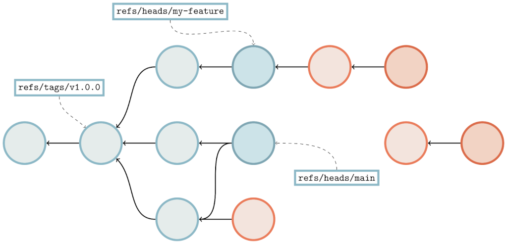
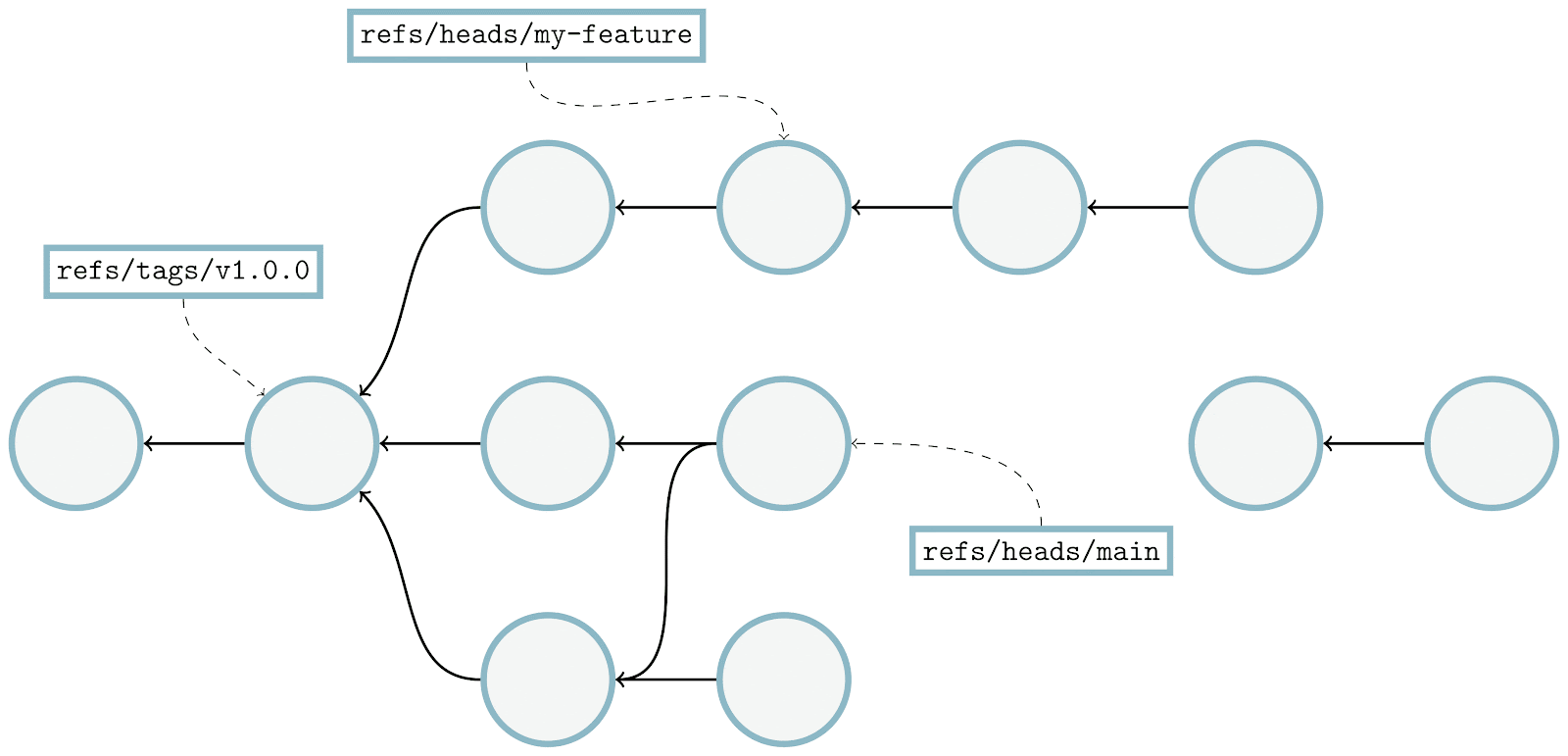
Here, we’re looking at a sample object graph. For simplicity, I’m only showing commits (identified here as circles). Arrows point from commits to their parent(s). A few commits have boxes that are connected to them, which represent the tips of branches and tags.

The parts of the graph that are colored blue are reachable, and the red parts are considered unreachable. You’ll find that if you start at any branch or tag, and follow its arrows, that all commits along that path are considered reachable. Note that unreachable commits which have reachable ones as parents (in our diagram above, anytime an arrow points from a red commit to a blue one) are still considered unreachable, since they are not contained within any branch or tag.

Unreachable objects can also appear in clusters that are totally disconnected from the main object graph, as indicated by the two lone red commits towards the right-hand side of the image.

Pruning unreachable objects

Normally, unreachable objects stick around in your repository until they are either automatically or manually cleaned up. If you’ve ever seen the message, “Auto packing the repository for optimum performance,” in your terminal, Git is doing this for you in the background. You can also trigger garbage collection manually by running:

$ git gc --prune=<date>

That tells Git to trigger a garbage collection and remove unreachable objects. But observant readers might notice the optional <date> parameter to the --prune flag. What is that? The short answer is that Git allows you to restrict which objects get permanently deleted based on the last time they were written. But to fully explain, we first need to talk a little bit about a race condition that can occur when removing objects from a Git repository.

Object deletion raciness

Normally, deleting an unreachable object from a Git repository should not be a notable event. Since the object is unreachable, it’s not part of any branch or tag, and so deleting it doesn’t change the repository’s reachable state. In other words, removing an unreachable object from a repository should be as simple as:

1. Repacking the repository to remove any copies of the object in question (and recomputing any deltas that are based on that object).
2. Removing any loose copies of the object that happen to exist.
3. Updating any additional indexes (like the multi-pack index, or commit-graph) that depend on the (now stale) packs that were removed.

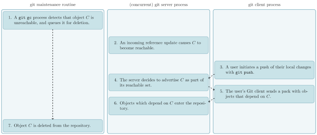
The racy behavior occurs when a repository receives one or more pushes during this process. The main culprit is that the server advertises its objects at a different point in time from processing the objects that the client sent based on that advertisement.

Consider what happens if Git decides (as part of running a git gc operation) that it wants to delete some unreachable object C. If C becomes reachable by some background reference update (e.g., an incoming push that creates a new branch pointing at C), it will then be advertised to any incoming pushes. If one of these pushes happens before C is actually removed, then the repository can end up in a corrupt state. Since the pusher will assume C is reachable (since it was part of the object advertisement), it is allowed to include objects that either reference or depend on C, without sending C itself. If C is then deleted while other reachable parts of the repository depend on it, then the repository will be left in a corrupt state.

Suppose the server receives that push before proceeding to delete C. Then, any objects from the incoming push that are related to it would be immediately corrupt. Reachable parts of the repository that reference C are no longer closed² over reachability since C is missing. And any objects that are stored as a delta against C can no longer be inflated for the same reason.

In case that was confusing, the above figure should help clear things up. The general idea is that one side (responsible for garbage collecting the repository) decides that a certain object is unreachable, while another side makes that object reachable and accepts an incoming push based on that object—before the original side ultimately deletes that (now-reachable) object—leaving the repository in a corrupt state.

Mitigating object deletion raciness

Git does not completely prevent this race from happening. Instead, it works around the race by gradually expiring unreachable objects based on the last time they were written. This explains the mysterious --prune=<date> option from a few sections ago: when garbage collecting a repository, only unreachable objects which haven’t been written since <date> are removed. Anything else (that is, the set of objects that have been written at least once since <date>) are left around.

The idea is that objects which have been written recently are more likely to become reachable again in the future, and would thus be more likely to be susceptible to the kind of race we talked about above if they were to be pruned. Objects which haven’t been written recently, on the other hand, are proportionally less likely to become reachable again, and so they are safe (or, at least, safer) to remove.

This idea isn’t foolproof, and it is certainly possible to run into the race we talked about earlier. We’ll discuss one such scenario towards the end of this post (along with the way we worked around it). But in practice, this strategy is simple and effective, preventing most instances of potential repository corruption.

Storing loose unreachable objects

But one question remains: how does Git keep track of the age of unreachable objects which haven’t yet aged out of the repository?

The answer, though simple, is at the heart of the problem we’re trying to solve here. Unreachable objects which have been written too recently to be removed from the repository are stored as loose objects, the individual object files stored in .git/objects. Storing these unreachable objects individually means that we can rely on their stat() modification time (hereafter, mtime) to tell us how recently they were written.

But this leads to an unfortunate problem: if a repository has many unreachable objects, and a large number of them were written recently, they must all be stored individually as loose objects. This is undesirable for a number of reasons:

• Pairs of unreachable objects that share a vast majority of their contents must be stored separately, and can’t benefit from the kind of deduplication offered by packfiles. This can cause your repository to take up much more space than it otherwise would.
• Having too many files (especially too many in a single directory) can lead to performance problems, including exhausting your system’s available inodes in the extreme case, leaving you unable to create new files, even if there may be space available for them.
• Any Git operation which has to scan through all loose objects (for example, git repack -d, which creates a new pack containing just your repository’s unpacked objects) will slow down as there are more files to process.

It’s tempting to want to store all of a repository’s unreachable objects into a single pack. But there’s a problem there, too. Since all of the objects in a single pack share the same mtime (the mtime of the *.pack file itself), rewriting any single unreachable object has the effect of updating the mtimes of all of a repository’s unreachable objects. This is because Git optimizes out object writes for packed objects by simply updating the mtime of any pack(s) which contain that object. This makes it nearly impossible to expire any objects out of the repository permanently.

Cruft packs

To solve this problem, we turned to a long-discussed idea on the Git mailing list: cruft packs. The idea is simple: store an auxiliary list of mtime data alongside a pack containing just unreachable objects. To garbage collect a repository, Git places the unreachable objects in a pack. That pack is designated as a “cruft pack” because Git also writes the mtime data corresponding to each object in a separate file alongside that pack. This makes it possible to update the mtime of a single unreachable object without changing the mtimes of any other unreachable object.

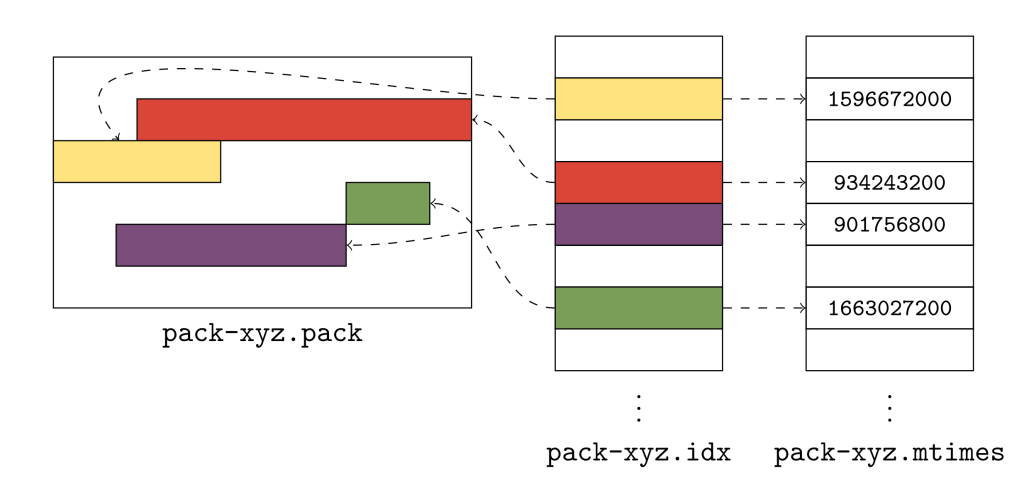
To give you a sense of what this looks like in practice, here’s a small example:

The above figure shows a pack of Git objects (represented by rectangles of different colors), its pack index, and the new .mtimes file. Together, these three files make up what Git calls a “cruft pack,” and it’s what allows Git to store unreachable objects together, without needing a single file for each object.

So, how do they work? Git uses the cruft pack to store a collection of object mtimes together in an array stored in the *.mtimes file. In order to discover the mtime for an individual object in a pack, Git first does a binary search on the pack’s index to discover that object’s lexicographic index. Git can then use that offset to read a 4-byte, unsigned integer in the .mtimes file. The .mtimes file contains a table of integers (one for each object in the associated *.pack file), each representing an epoch timestamp containing that object’s mtime. In other words, the *.mtimes file has a table of numbers, where each number represents an individual object’s mtime, encoded as a number of seconds since the Unix epoch.

Crucially, this makes it possible to store all of a repository’s unreachable objects together in a single pack, without having to store them as individual loose objects, bypassing all of the drawbacks we discussed in the last section. Moreover, it allows Git to update the mtime of a single unreachable object, without inadvertently triggering the same update across all unreachable objects.

Since Git doesn’t portably support updating a file in place, updating an object’s mtime (a process which Git calls “freshening”) takes place by writing a separate copy of that object out as a loose file. Of course, if we had to freshen all objects in a cruft pack, we would end up in a situation no better than before. But such updates tend to be unlikely in practice, and so writing individual copies of a small handful of unreachable objects ends up being a reasonable trade off most of the time.

Generating cruft packs

Now that we have introduced the concept of cruft packs, the question remains: how does Git generate them?

Despite being called git gc (short for “garbage collection”), running git gc does not always result in deleting unreachable objects. If you run git gc --prune=never, then Git will repack all reachable objects and move all unreachable objects to the cruft pack. If, however, you run git gc --prune=1.day.ago, then Git will repack all reachable objects, delete any unreachable objects that are older than one day, and repack the remaining unreachable objects into the cruft pack.

This is because of Git’s treatment of unreachable parts of the repository. While Git only relies on having a reachability closure over reachable objects, Git’s garbage collection routine tries to leave unreachable parts of the repository intact to the extent possible. That means if Git encounters some unreachable cluster of objects in your repository, it will either expire all or none of those objects, but never some subset of them.

We’ll discuss how cruft packs are generated with and without object expiration in the two sections below.

Cruft packs without object expiration

When generating a cruft pack with an object expiration of --date=never, our only goal is to collect all unreachable objects together into a single cruft pack. Broadly speaking, this occurs in three steps:

1. Starting at all of the branches and tags, generate a pack containing only reachable objects.
2. Looking at all other existing packs, enumerate the list of objects which don’t appear in the new pack of reachable objects. Create a new pack containing just these objects, which are unreachable.
3. Delete the existing packs.

If any of that was confusing, don’t worry: we’ll break it down here step by step. The first step to collecting a repository’s unreachable objects is to figure out the parts of it that are reachable. If you’ve ever run git repack -A, this is exactly how that command works. Git starts a reachability traversal beginning at each of the branches and tags in your repository. Then it traverses back through history by walking from commits to their parents, trees to their sub-trees, and so on, marking every object that it sees along the way as reachable.

Here, we’re showing the same commit graph from earlier in the post. Git’s goal at this point is simply to mark every reachable object that it sees, and it’s those objects that will become the contents of a new pack containing just reachable objects. Git starts by examining each reference, and walking from a commit to its parents until it either finds a commit with no parents (indicating the beginning of history), or a commit that it has already marked as reachable.

In the above, the commit being walked is highlighted in dark blue, and any commits marked as reachable are marked in green. At each step, the commit currently being visited gets marked as reachable, and its parent(s) are visited in the next step. By repeating this process among all branches and tags, Git will mark all reachable objects in the repository.

We can then use this set of objects to produce a new pack containing all reachable objects in a repository. Next, Git needs to discover the set of objects that it didn’t mark in the previous stage. A reasonable first approach might be to store the IDs of all of a repository’s objects in a set, and then remove them one by one as we mark objects reachable along our walk.

But this approach tends to be impractical, since each object will require a minimum of 20 bytes of memory in order to insert into this set. At the time of writing, the linux.git repository contains nearly nine million objects, which would require nearly 180 MB of memory just to write out all of their object IDs.

Instead, Git looks through all of the objects in all of the existing packs, checking whether or not each is contained in the new pack of reachable objects. Any object found in an existing pack which doesn’t appear in the reachable pack is automatically included in the cruft pack.

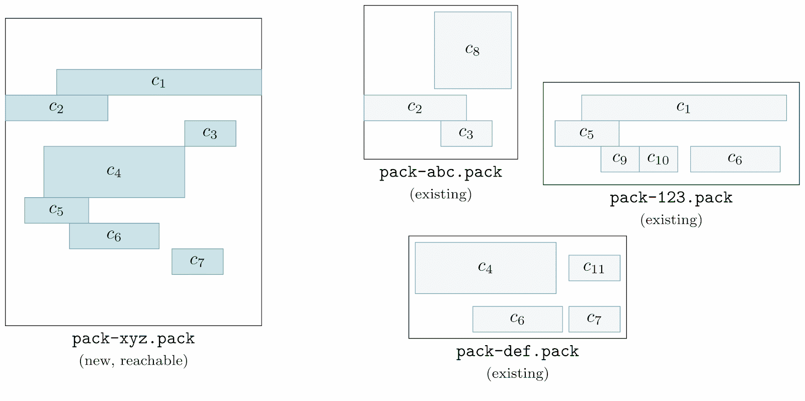
Here, we’re going one by one among all of the pre-existing packs (here, labeled as pack-abc.pack, pack-def.pack, and pack-123.pack) and inspecting their objects one at a time. We first start with object c8, looking through the reachable pack (denoted as pack-xyz.pack) to see if any of its objects match c8. Since none do, c8 is marked unreachable (which we represent by filling the object with a red background).

This process is repeated for each object in each existing pack. Once this process is complete, all objects that existed in the repository before starting a garbage collection are marked either green, or red (indicating that they are either reachable, or unreachable, respectively).

Git can then use the set of unreachable objects to generate a new pack, like below:

This pack (on the far right of the above image, denoted pack-cruft.pack) contains exactly the set of unreachable objects present in the repository at the beginning of garbage collection. By keeping track of each unreachable object’s mtime while marking existing objects, Git has enough data to write out a *.mtimes file in addition to the new pack, leaving us with a cruft pack containing just the repository’s unreachable objects.

Here, we’re eliding some technical details about keeping track of each object’s mtime along the way, for brevity and simplicity. The routine is straightforward, though: each time we discover an object, we mark its mtime based on how we discovered the object.

• If an object is found in a packfile, it inherits its mtime from the packfile itself.
• If an object is found as a loose object, its mtime comes from the loose object file.
• And if an object is found in an existing cruft pack, its mtime comes from reading the cruft pack’s *.mtimes file at the appropriate index.

If an object is seen more than once (e.g., an unreachable object stored in a cruft pack was freshened, resulting in another loose copy of the object), the mtime which is ultimately recorded in the new cruft pack is the most recent mtime of all of the above.

Cruft packs with object expiration

Generating cruft packs where some objects are going to expire out of the repository follows a similar, but slightly trickier approach than in the non-expiring case.

Doing a garbage collection with a fixed expiration is known as “pruning.” This essentially boils down to asking Git to pack the contents of a repository into two packfiles: one containing reachable objects, and another containing any unreachable objects. But, it also means that for some fixed expiration date, any unreachable objects which have an mtime older than the expiration date are removed from the repository entirely.

The difficulty in this case stems from a fact briefly mentioned earlier in this post, which is that Git attempts to prevent connected clusters of unreachable objects from leaving the repository if some, but not all, of their objects have aged out.

To make things clearer, here’s an example. Suppose that a repository has a handful of blob objects, all connected to some tree object, and all of these objects are unreachable. Assuming that they’re all old enough, then they will all expire together: no big deal. But what if the tree isn’t old enough to be expired? In this case, even though the blobs connected to it could be expired on their own, Git will keep them around since they’re connected to a tree with a sufficiently recent mtime. Git does this to preserve the repository’s reachability closure in case that tree were to become reachable again (in which case, having the tree and its blobs becomes important).

To ensure that Git preserves any unreachable objects which are reachable from recent objects Git handles this case of cruft pack generation slightly differently. At a high level, it:

1. Generates a candidate list of cruft objects, using the same process as outlined in the previous section.
2. Then, to determine the actual list of cruft objects to keep around, it performs a reachability traversal using all of the candidate cruft objects, adding any object it sees along the way to the cruft pack.

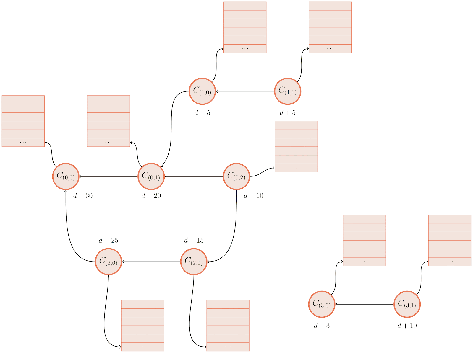
To make things a little clearer, here’s an example:

After determining the set of unreachable objects (represented above as colored red) Git does a reachability traversal from each entry point into the graph of unreachable objects. Above, commits are represented by circles, trees by rectangles, and tree entries as rows within the larger rectangles. The mtimes are written below each commit.

For now, let’s assume our expiration date is d, so any object whose mtime is greater than d must stay (despite being unreachable), and anything older than d can be pruned. Git traverses through each entry and asks, “Is this object old enough to be pruned?” When the answer is “yes” Git leaves the object alone and moves on to the next entry point. When the answer is “no,” however, (ie., Git is looking at an unreachable object whose mtime is too recent to prune), Git marks that object as “rescued” (indicated by turning it green) and then continues its traversal, marking any reachable objects as rescued.

Objects that are rescued during this pass are written to the cruft pack, preserving their existence in the repository, leaving them to either continue to age, or have their mtimes updated before the next garbage collection.

Let’s take a closer look at the example above. Git starts by looking at object C(1,1), and notice that its mtime is d+5, meaning that (since it happens after our expiration time, d) it is too new to expire. That causes Git to start a reachability traversal beginning at C(1,1), rescuing every object it encounters along the way. Since many objects are shared between multiple commits, rescuing an object from a more recent part of the graph often ends up marking older objects as rescued, too.

After finishing the rescuing pass focused on C(1,1), Git moves on to look at C(0,2). But this commit’s mtime is d-10, which is before our expiration cutoff of d, meaning that it is safe to remove. Git can skip looking at any objects reachable from this commit, since none of them will be rescued.

Finally, Git looks at another connected cluster of the unreachable object graph, beginning at C(3,1). Since this object has an mtime of d+10, it is too new to expire, so Git performs another reachability traversal, rescuing it and any objects reachable from it.

Notice that in the final graph state that the main cluster of commits (the one beginning with C(0,2)) is only partially rescued. In fact, only the objects necessary to retain a reachability closure over the rescued objects among that cluster are saved from being pruned. So even though, for example, commit C(2,1) has only part of its tree entries rescued, that is OK since C(2,1) itself will be pruned (hence any non-rescued tree entries connected to it are unimportant and will also be pruned).

Putting it all together

Now that Git can generate a cruft pack and perform garbage collection on a repository with or without pruning objects, it was time to put all of the pieces together and submit the patches to the open-source Git project.

Other Git sub-commands, like repack, and gc needed to learn about cruft packs, and gain command-line flags and configuration knobs in order to opt-in to the new behavior. With all of the pieces in place, you can now trigger a garbage collection by running either:

$ git gc --prune=1.day.ago --cruft

or

$ git repack -d --cruft --cruft-expiration=1.day.ago

to repack your repository into a reachable pack, and a cruft pack containing unreachable objects whose mtimes are within the past day. More details on the new command-line options and configuration can be found here, here, here, and here.

GitHub submitted the entirety of the patches that comprise cruft packs to the open-source Git project, and the results were released in v2.37.0. That means that you can use the same tools as what we run at GitHub on your own laptop, to run garbage collection on your own repositories.

For those curious about the details, you can read the complete thread on the mailing list archive here.

Cruft packs at GitHub

After a lengthy process of testing to ensure that using cruft packs was safe to carry out across all repositories on GitHub, we deployed and enabled the feature across all repositories. We kept a close eye on repositories with large numbers of unreachable objects, since the process of breaking any deltas between reachable and unreachable objects (since the two are now stored in separate packs, and object deltas cannot cross pack boundaries) can cause the initial cruft pack generation to take a long time. A small handful of repositories with many unreachable objects needed more time to generate their very first cruft pack. In those instances, we generated their cruft packs outside of our normal repository maintenance jobs to avoid triggering any timeouts.

Now, every repository on GitHub and in GitHub Enterprise (in version 3.3 and newer) uses cruft packs to store their unreachable objects. This has made garbage collecting repositories (especially busy ones with many unreachable objects) tractable where it often required significant human intervention before. Before cruft packs, many repositories which required clean up were simply out of our reach because of the possibility of creating an explosion of loose objects which could derail performance for all repositories stored on a fileserver. Now, garbage collecting a repository is a simple task, no matter its size or scale.

During our testing, we ran garbage collection on a handful of repositories, and got some exciting results. For repositories that regularly force-push a single commit to their main branch (leaving a majority of their objects unreachable), their on-disk size dropped significantly. The most extreme example we found during testing caused a repository which used to take 186 gigabytes to store shrink to only take 2 gigabytes of space.

On github/github, GitHub’s main codebase, we were able to shrink the repository from around 57 gigabytes to 27 gigabytes. Even though these savings are more modest, the real payoff is in the objects we no longer have to store. Before garbage collecting, each replica of this repository had nearly 60 million objects, including years of test-merges, force-pushes, and all kinds of sources of unreachable objects. Each of these objects contributed to the I/O cost of repacking this repository. After garbage collecting, only 11.8 million objects remained. Since each object in a repository requires around 150 bytes of memory during repacking, we save around 7 gigabytes of RAM during each maintenance routine.

Limbo repositories

Even though we can easily garbage collect a repository of any size, we still have to navigate the inherent raciness that we described at the beginning of this post.

At GitHub, our approach has been to make this situation easy to recover from automatically instead of preventing it entirely (which would require significant surgery to much of Git’s code). To do this, our approach is to create a “limbo” repository whenever a pruning garbage collection is done. Any objects which get expired from the main repository are stored in a separate pack in the limbo repository. Then, the process to garbage collect a repository looks something like:

1. Generate a cruft pack of recent unreachable objects in the main repository.
2. Generate a second cruft pack of expired unreachable objects, stored outside of the main repository, in the “limbo” repository.
3. After garbage collection has completed, run a git fsck in the main repository to detect any object corruption.
4. If any objects are missing, recover them by copying them over from the limbo repository.

The process for generating a cruft pack of expired unreachable objects boils down to creating another cruft pack (using exactly the same process we described earlier in this post), with two caveats:

• The expiration cutoff is set to “never” since we want to keep around any objects which we did expire in the previous step.
• The original cruft pack is treated as a pack containing reachable objects since we want to ignore any unreachable objects which were too recent to expire (and, thus, are stored in the cruft pack in the main repository).

We have used this idea at GitHub with great success, and now treat garbage collection as a hands-off process from start to finish. The patches to implement this approach are available as a preliminary RFC on the Git mailing list here.

Thank you

This work would not have been possible without generous review and collaboration from engineers from within and outside of GitHub. The Git Systems team at GitHub were great to work with while we developed and deployed cruft packs. Special thanks to Torsten Walter, and Michael Haggerty, who played substantial roles in developing limbo repositories.

Outside of GitHub, this work would not have been possible without careful review from the open-source Git community, especially Derrick Stolee, Jeff King, Jonathan Tan, Jonathan Nieder, and Junio C Hamano. In particular, Jeff King contributed significantly to the original development of many of the ideas discussed above.

Notes