Post Syndicated from Ramesh Kandasamy original https://aws.amazon.com/blogs/big-data/accelerate-apache-hive-read-and-write-on-amazon-emr-using-enhanced-s3a/
Improving Apache Hive read and write performance on Amazon EMR is crucial for organizations dealing with large-scale data analytics and processing. When queries execute faster, businesses can make data-driven decisions more quickly, reduce time-to-insight, and optimize their operational costs. In today’s competitive landscape, where real-time analytics and interactive querying are becoming standard requirements, every millisecond of latency reduction can significantly impact business outcomes.
The Amazon EMR runtime for Apache Hive is a performance-optimized runtime that is 100% API compatible with open source Apache Hive. It offers faster out-of-the-box performance than Apache Hive through improved query plans, faster queries, and tuned defaults. Amazon EMR on Amazon EC2 and Amazon EMR Serverless use this optimized runtime, which is 1.5 times faster for read queries than EMR 7.0 based on an industry standard benchmark derived from TPC-DS at 3 TB scale and 3 times faster for write queries.
Apache Hive on Amazon EMR added over 10 features from Amazon EMR 7.0 to Amazon EMR 7.10 releases and continuing. These improvements are turned on by default and are 100% API compatible with Apache Hive. Some of the improvements include:
- Default EMR enhanced S3A file system implementation for Apache Hive on Amazon EMR
- Amazon EMR enhanced S3A zero-rename feature with 3-times improved write performance
- Read query performance parity with EMR File System (EMRFS)
- AWS Lake Formation support with Amazon EMR enhanced S3A
- Fine-tuned file listing process for file formats including Parquet, Text, CSV, and so on
- Async record reader initialization
- Improvements to Tez task preemption
- Fine-tuned locality during container reuse
- Improved Tez relaxed locality
- Improvements with split computation for ORC file formats
Transitioning from EMRFS to Amazon EMR enhanced S3A
The storage interface of Amazon EMR has evolved through two implementations: EMRFS and S3A. EMRFS, a proprietary Amazon Simple Storage Service (Amazon S3) connector developed by Amazon, has been the default filesystem for Amazon EMR since its early days, offering AWS-specific optimizations such as Consistent View for handling eventual consistency in Amazon S3, specialized performance tuning for the AWS environment, and seamless integration with AWS services through AWS Identity and Access Management (IAM) roles. On the other hand, S3A emerged from the Apache Hadoop open source community as a standard S3 connector and has evolved significantly through continuous improvements, performance optimizations, and enhanced S3 feature support. While EMRFS was designed specifically for optimal S3 access within Amazon EMR, S3A’s community-driven development has closed the performance gap with proprietary implementations.
Advantages of using enhanced S3A in Apache Hive on Amazon EMR
The transition from EMRFS to Amazon EMR enhanced S3A as the default filesystem in Amazon EMR 7.10 marks a strategic shift toward open source standardization while maintaining performance parity and adding benefits like improved portability and community support.
Based on the Amazon EMR HBase on Amazon S3 transitioning to EMR S3A with comparable EMRFS performance blog post, S3A in Amazon EMR Hive offers significant advantages over EMRFS, using modern AWS technologies and advanced storage capabilities.
- The integration of AWS SDK v2 brings improved performance through non-blocking I/O, async clients, and better credential management.
- S3A provides comprehensive support for Amazon S3 Glacier (Amazon S3 Glacier)and Amazon S3 Glacier Deep Archive, enabling cost-effective data lifecycle management and efficient handling of archival data for analytics.
- It offers enhanced infrastructure flexibility with AWS Outposts support for on-premises deployments and custom endpoint support for Amazon S3-compatible storage systems, facilitating hybrid and multi-cloud architectures.
- Performance is significantly boosted with Amazon S3 Express One Zone support, providing single-digit millisecond access for latency-sensitive analytics and interactive data exploration.
- S3A introduces vector reads, allowing efficient access to columnar data formats by batching multiple non-contiguous byte ranges into a single S3
GETrequest, reducing I/O overhead and improving query performance. - The prefetching feature in S3A optimizes sequential read performance by proactively fetching data, enhancing throughput and reducing latency for large-scale data processing tasks.
- S3A’s enhanced delegation token support, a result of AWS SDK v2 integration, provides flexible authentication mechanisms including support for web identity tokens and federated identity systems.
These advanced features make S3A a more versatile, efficient, and performance-oriented choice for organizations using Hive on Amazon EMR, particularly those requiring sophisticated data management and analytics capabilities across diverse infrastructure environments.
Read queries performance comparison
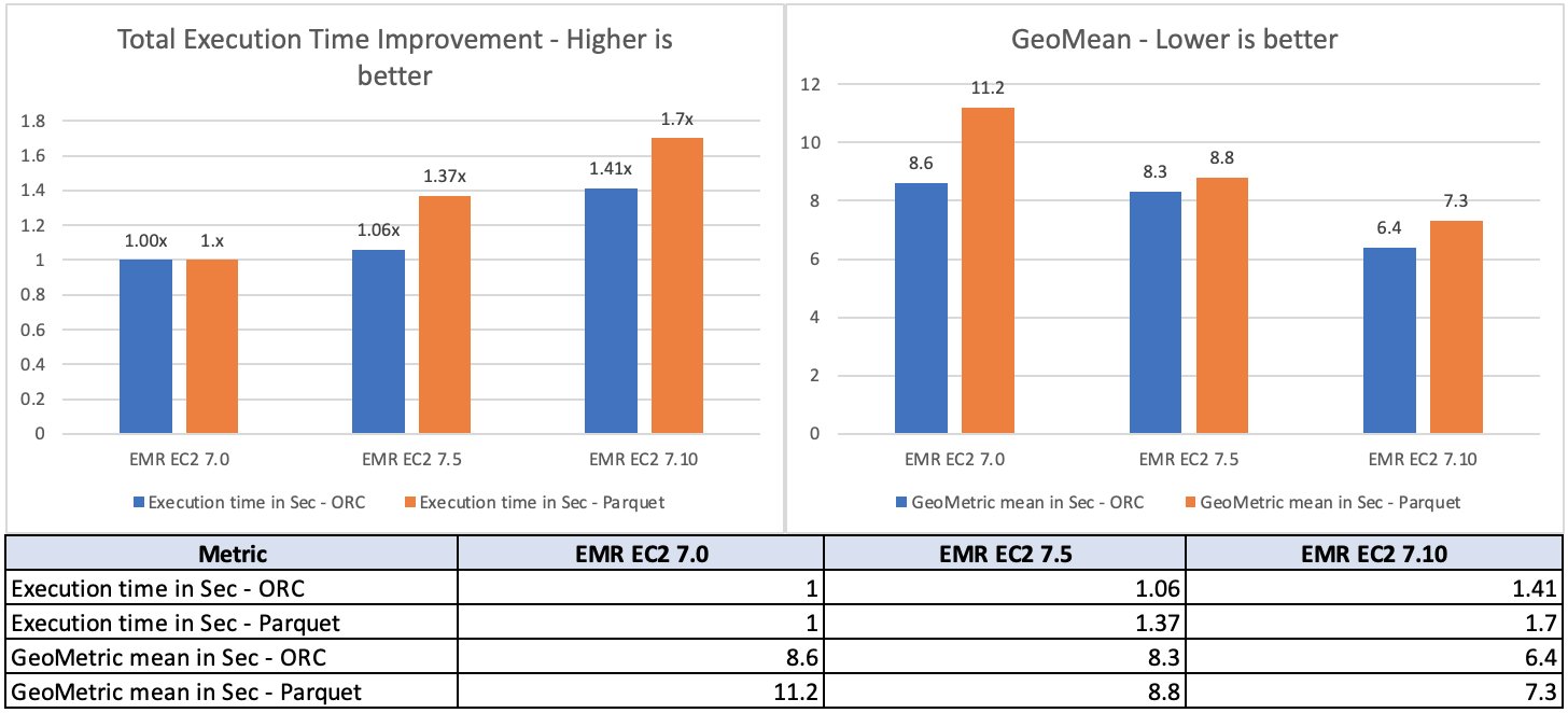
To evaluate the Amazon EMR Hive engine performance, we ran benchmark tests with the 3 TB TPC-DS datasets. We used Amazon EMR Hive clusters for benchmark tests on Amazon EMR and installed Apache Hive 3.1.3 on Amazon Elastic Compute Cloud (Amazon EC2) clusters designated for open source software (OSS) benchmark runs. We ran tests on separate EC2 clusters comprised of 16 m5.8xlarge instances for each of Apache Hive 3.1.3, Amazon EMR 7.0.0, Amazon EMR 7.5.0 and Amazon EMR 7.10.0. The primary node has 32 vCPU and 128 GB memory, and 16 worker nodes have a total of 512 vCPU and 2048 GB memory. We tested with Amazon EMR defaults to highlight the out-of-the-box experience and tuned Apache Hive with the minimal settings needed to provide a fair comparison.
For the source data, we chose the 3 TB scale factor, which contains 17.7 billion records, approximately 924 GB of compressed data in Parquet file format and ORC file format. The fact tables are partitioned by the date column, which consists of partitions ranging from 200–2,100. No statistics were pre-calculated for these tables. A total of 104 Hive SQL queries were run in five iterations sequentially and an average of each query’s runtime in these five iterations was used for comparison. The average of the five iterations’ runtime on Amazon EMR 7.10 was approximately 1.5 times faster than Amazon EMR 7.0. The following figure illustrates the total runtimes in seconds.
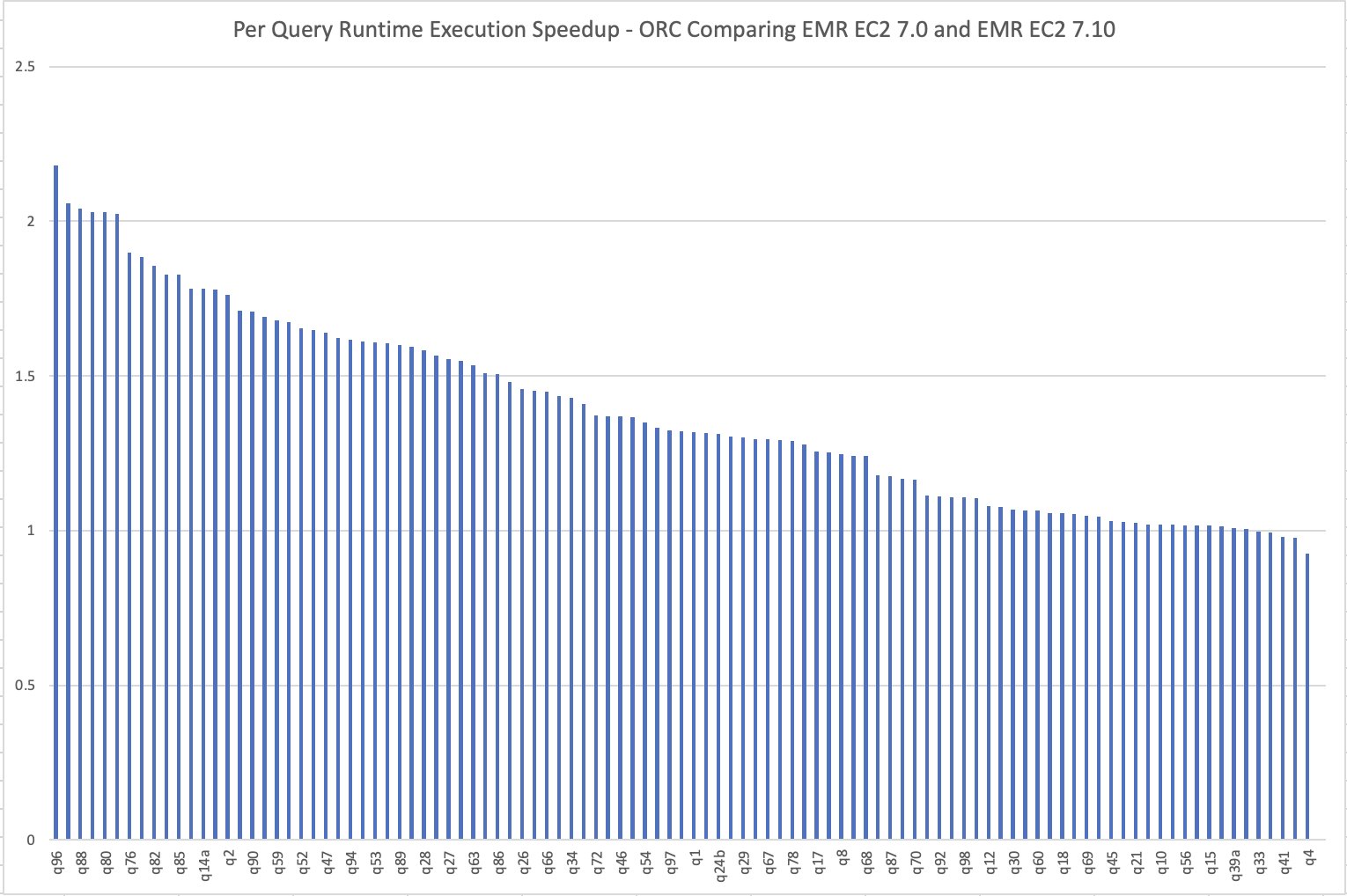
The per-query speedup on Amazon EMR 7.10 when compared to Amazon EMR 7.0 is illustrated in the following chart. The horizontal axis represents queries in the TPC-DS 3 TB benchmark ordered by the Amazon EMR speedup descending and the vertical axis shows the speedup of queries due to the Amazon EMR runtime.
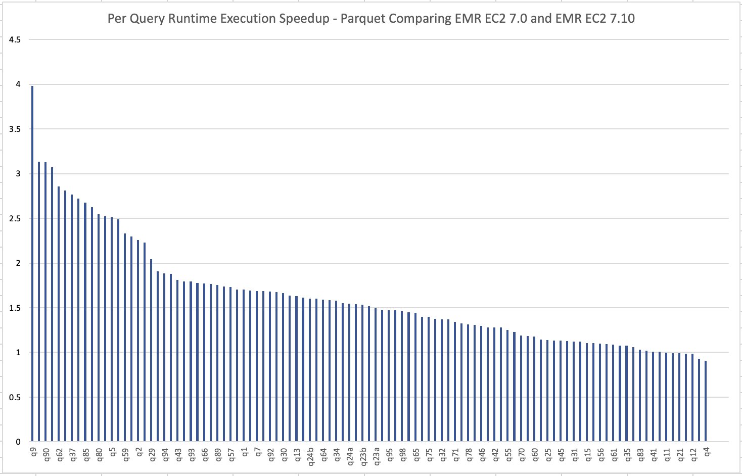
The below image illustrates the per-query speedup on Amazon EMR 7.10 when compared to Amazon EMR 7.0 for Parquet files.
Read cost comparison
Our benchmark outputs the total runtime and geometric mean figures to measure the Hive runtime performance by simulating a real-world complex decision support use case. The cost metric can provide us with additional insights. Cost estimates are computed using the following formulas. They factor in Amazon EC2, Amazon Elastic Block Store (Amazon EBS), and Amazon EMR costs, but don’t include Amazon S3 GET and PUT costs.
- Amazon EC2 cost (including SSD cost) = number of instances * m5.8xlarge hourly rate * job runtime in hours
- 8xlarge hourly rate = $1.536 per hour
- Root Amazon EBS cost = number of instances * Amazon EBS per GB-hourly rate * root EBS volume size * job runtime in hours
- Amazon EMR cost = number of instances * m5.8xlarge Amazon EMR cost * job runtime in hours
- 8xlarge Amazon EMR cost = $0.27 per hour
- Total cost = Amazon EC2 cost + root Amazon EBS cost + Amazon EMR cost
Based on the calculation, the Amazon EMR 7.10 benchmark result demonstrates a 33% improvement in job cost compared to Amazon EMR 7.0.
| Metric | Amazon EMR 7.0.0 | Amazon EMR 7.10.0 |
| Runtime in hours | 2.86 | < 2.00 |
| Number of EC2 instances | 17 | 17 |
| Amazon EBS Size | 20gb | 20gb |
| Amazon EC2 cost | $78.34 | $52.22 |
| Amazon EBS cost | $0.01 | $0.01 |
| Amazon EMR cost | $14.58 | $9.72 |
| Total cost | $92.93 | $61.96 |
| Cost Savings | Baseline | Amazon EMR 7.10.0 is 33% better than Amazon EMR 7.0.0 |
Hive write committers performance comparison
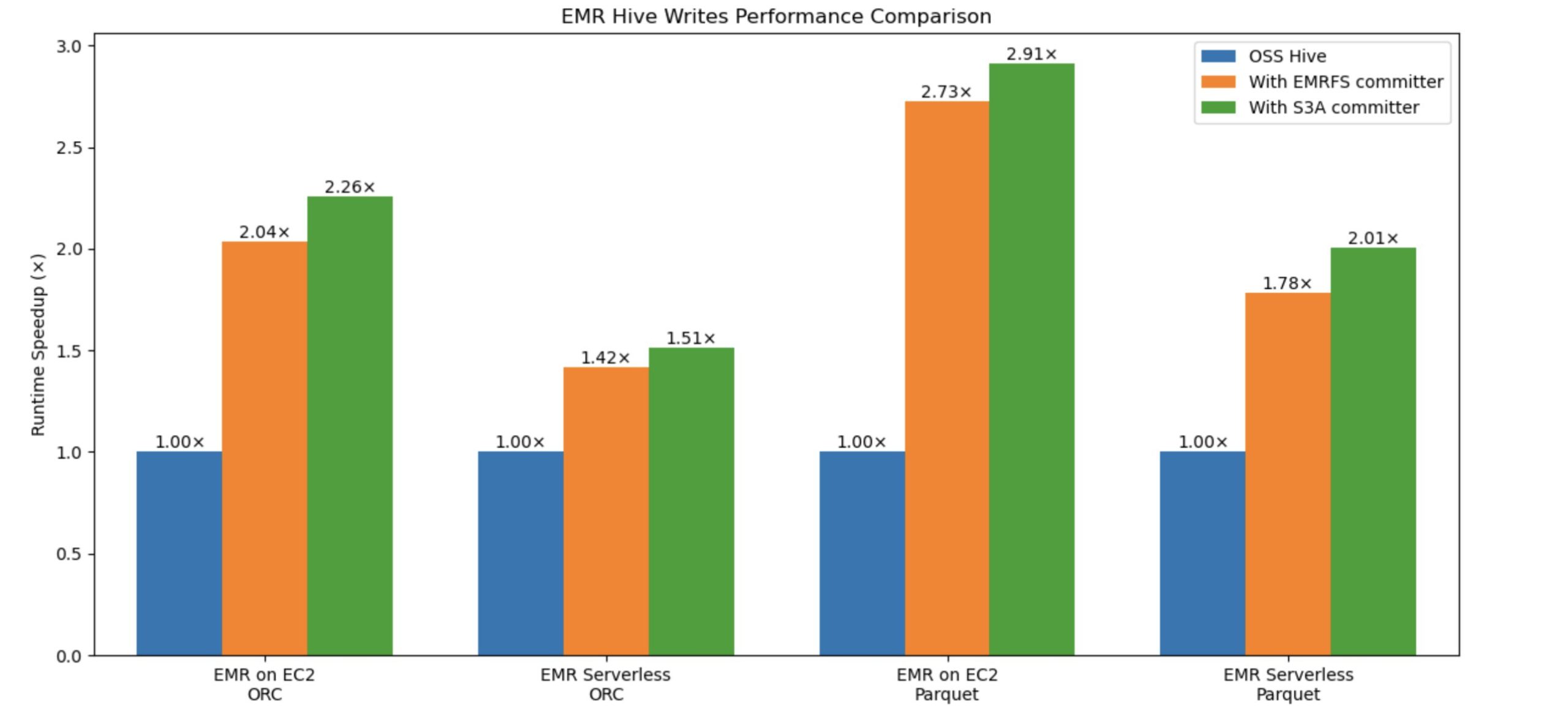
Amazon EMR introduced a new committer to enhance Hive write performance on Amazon S3 up to 2.91 times faster. The existing Hive EMRFS S3-optimized committer, eliminates rename operations by writing data directly to the output location and only commits files at job completion to help enforce failure resilience. It implements a modified file naming convention that includes a query ID suffix. The new, Hive S3A-optimized committer, was developed to bring similar zero-rename capabilities to Hive on S3A, which previously lacked this feature. Built on OSS Hadoop’s Magic Committer, it eliminates unnecessary file movements during commit phases using S3 multipart upload (MPU) operations. This newer committer not only matches but exceeds EMRFS performance, delivering faster Hive write query execution while reducing S3 API calls, resulting in improved efficiency and cost savings for customers. Both committers effectively address the performance bottleneck caused by rename operations in Hive, with the S3A-optimized committer emerging as the superior solution.
Building on our previous blog post about the Amazon EMR Hive Zero Rename feature gains 15-fold write performance with EMRFS-optimized committer, we’ve achieved additional performance improvements in Hive write operations using the S3A optimized committer. We ran the comparison tests with and without the new committer and evaluated the write performance improvement. The benchmark used an insert overwrite query that joins two tables from a 3 TB TPC-DS ORC and Parquet dataset.
The following graph compares Hive write query total runtime speedup against ORC and Parquet formats. The y-axis denotes the speedup (total time taken with rename / total time taken by query with committer), and the x-axis denotes file formats and EMR deployment models. With the new S3A committer, the runtime speedup is better.
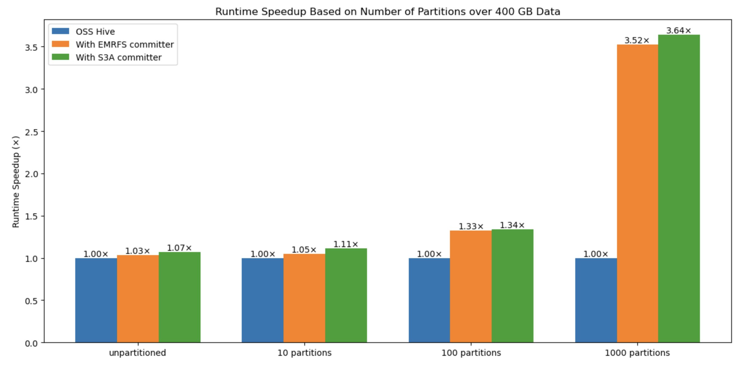
Understanding performance impact with different data sizes and number of files
To benchmark the performance impact with variable data sizes and number of files, we also evaluated the solution with various types, such as size of data (10 files –unpartitioned, 10 partitions, 100 partitions, 1000 partitions), number of files, and number of partitions: The results show that the number of files written is the critical factor for performance improvement when using this new committer in comparison to the default Hive commit logic and EMRFS committer.
In the following graph, the y-axis denotes the runtime speedup (total time taken with rename / total time taken by query with committer), and the x-axis denotes the number of partitions. We observed that as the number of partitions increases, the committer performs better because of avoiding multiple expensive rename operations in Amazon S3.
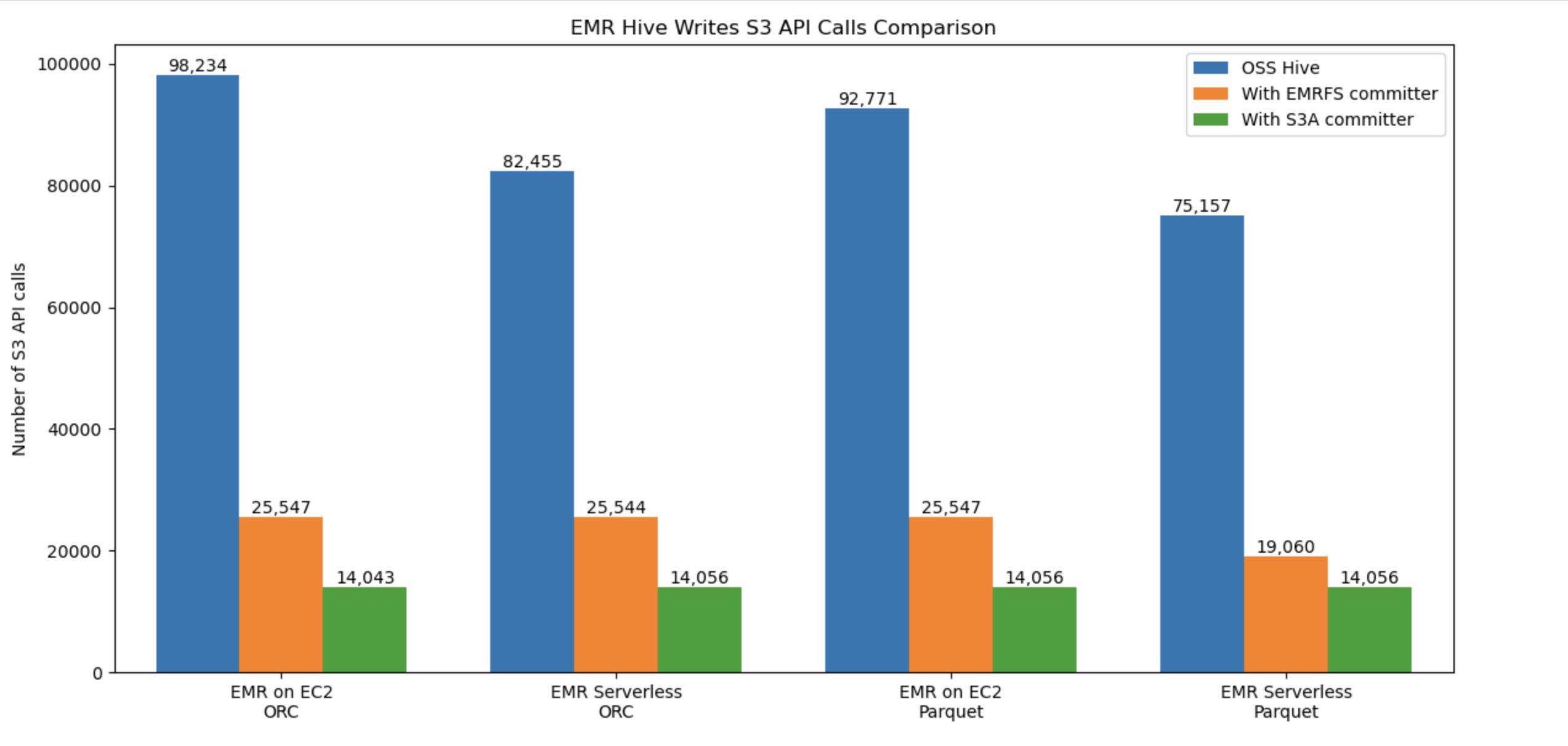
Write cost comparison
The following graph compares the number of overall Amazon S3 API calls for Hive write workflow against ORC and Parquet formats. The benchmark used an insert overwrite query that joins two tables from a 3 TB TPC-DS ORC, Parquet datasets on both Amazon EMR EC2 and Amazon EMR Serverless. With the new committer, the S3 usage cost is better(lower).
Limitations with Hive S3A zero-rename feature
This committer will not be used, and default Hive commit logic will be applied in the following scenarios:
- When merge small files (
hive.merge.tezfiles) is enabled. - When using Hive ACID tables.
- When partitions are distributed across file systems such as HDFS and Amazon S3.
Summary
Amazon EMR continues to improve the Amazon EMR runtime for Apache Hive, leading to a performance improvement year-over-year and additional features for big data customers to run their analytics workload in cost effective manner. More importantly, the transition to S3A brings additional benefits such as improved standardization, better portability, and stronger community support, while maintaining the robust performance levels established by EMRFS. We recommend that you stay up to date with the latest Amazon EMR release to take advantage of the latest performance and feature benefits.
To keep up to date, subscribe to the Big Data Blog RSS feed to learn more about Amazon EMR runtime for Apache Hive, configuration best practices, and tuning advice.