Tag Archives: regression

Predicting Risk in Content Launches: How Data-Driven Insights can Transform Launch Planning

Post Syndicated from Netflix Technology Blog original https://medium.com/netflix-techblog/predicting-risk-in-content-launches-how-data-driven-insights-can-transform-launch-planning-587b1f2de928

by Emily Gill

Each year, we bring the Analytics Engineering community together for an Analytics Summit — a multi-day internal conference to share analytical deliverables across Netflix, discuss analytic practice, and build relationships within the community. This post is one of several topics presented at the Summit highlighting the breadth and impact of Analytics work across different areas of the business.

Understanding Risk in Content Launches

Every title you see on Netflix goes through several key phases: Development, Pre-Production, Production/Principal Photography, Post-Production, and finally, Launch Preparation, all leading up to the Title Launch. Once Principal Photography wraps, the focus shifts in Post-Production from content creation to quality assurance and visual effects (if needed).

At the end of Post Production, Netflix receives the final audio and video files — often delivered as an IMF (Interoperable Master Format) — which triggers a flurry of Launch Preparation activities, focused on tasks such as the development of artwork and trailers, creation of subtitles, maturity ratings & quality control, that happen within a tight window and rely on having the finalized media assets in hand.

Some of this work can be kicked off earlier using a non-final version of the media called the Locked Cut, but since it’s not the absolute final deliverable, this presents a tradeoff: should our teams who prepare content for service wait for the more finalized IMF to begin their work, or start sooner with the unfinal Locked Cut? Waiting for the IMF risks a compressed timeline if it arrives late, while starting with the Locked Cut means teams may need to do additional conformance work if there are significant changes between the Locked Cut and the final IMF.

Identifying Gaps in Schedule Accuracy

To help navigate the decision of when to start launch preparation, our teams rely on estimated delivery dates for both the Locked Cut and IMF media assets, which are manually provided by content partners in production schedules. However, these schedules often have gaps in coverage and lack accuracy for both asset types (see Figure 1).
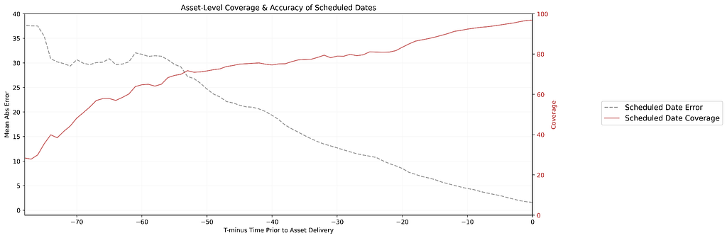
Figure 1. At an asset-level we generally see that scheduled date accuracy and coverage are lower at horizons further from asset delivery. As we approach delivery (moving towards the right on this plot) schedules become more accurate (errors decrease) adn coverage improves.

This isn’t unexpected — productions are dynamic, facing frequent changes, scheduling conflicts, and unforeseen obstacles that can shift timelines without warning. As a result, there’s a clear opportunity to leverage the wealth of production data we collect to predict the risk of schedule slips. By developing a predictive model, we aim to both fill in ETA gaps (providing asset delivery estimates when none exist) and improve the accuracy of existing ETAs compared to traditional manual schedules.

Correlation between Schedule Accuracy and Launch Misses

Our analysis reveals a strong correlation between scheduled inaccuracies and launch misses — instances where a title experiences delays. To quantify schedule inaccuracy, we created a metric called Accumulated Error Days (AED), which measures the cumulative deviation between estimated (scheduled or predicted) delivery dates and actual delivery dates over time. AED is calculated retrospectively as the area between the scheduled (grey line) or predicted (blue line) delivery dates and the actual delivery date (green line).

When we compare titles with at least one launch miss to those without, we find that mean AED is significantly higher in the group with launch misses. Notably, this effect is even more pronounced when we focus on the period closer to delivery — indicating that high AED (i.e., inaccurate schedules) in the final stretch before launch is especially correlated with launch misses, more so than AED accumulated over a longer timeline. These findings further motivate our efforts to improve schedule accuracy and reduce AED by leveraging rich production data and predictive modeling.

Modeling Time-to-Delivery

Our predictive models are designed as boosted tree regression models that predict the “days until” either media asset delivery for in-progress productions.

To power these models, we leverage a range of upstream data sources including production-level signals of progress, title metadata, and seasonal signals. We are able to predict the days until media asset delivery using daily update snapshots, allowing us to generate up-to-date predictions that reflect the latest state of each in-progress production. This means that we have each feature and what its value was as of each day of a production. Modeling with this snapshotted data enables us to generate up-to-date predictions as new information becomes available, build a flexible model that works across all production phases, and seamlessly incorporate dynamic features that evolve over time (Figure 2).
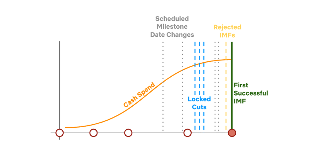
Figure 2. Hypothetical illustration of the evolving nature of production-related signals used in our models. Some signals are present throughout but dynamic, others are present at single moments in time during specific production phases. By capturing data in a snapshotted form, we’re able to build a flexible phase-agnostic model that leverages many different types of progress signals. This figure is illustrative only and does not depict actual Netflix financial or production data.

Evaluating Our Approach

Building a Comprehensive Metrics Suite

When evaluating the performance of the predictive models, we look across a suite of metrics to try to understand where and when predicted dates outperform scheduled dates. Among these are mean and median absolute error, relative to actual delivery, to understand the accuracy of our estimated dates. We also consider bias metrics, such as mean and median error, to understand if we are consistently over- or under-predicting the actual delivery. We calculate the standard deviation of our errors to understand if there are large shifts in the bulk of the distribution of errors. For the tails of our error distributions, we calculate the percentage of our absolute errors that are greater than x days to delivery.

For scheduled dates, we calculate coverage across various horizons to delivery. This is a value prop of the model; we’ve built the model in such a way that we can always provide a predicted date and recoup any coverage gaps that exist from scheduled dates alone.

Benchmarking Against Manual Scheduling

In a backtest, we observed significant improvements across all of our metrics and across most horizons from delivery. As an example, see Figure 3 which plots global mean absolute error (MAE) and shows large reductions in errors (greater accuracy) in predicted IMF and Locked dates as compared to scheduled dates. Additionally, we see large reductions in outliers from scheduled to predicted dates as well.
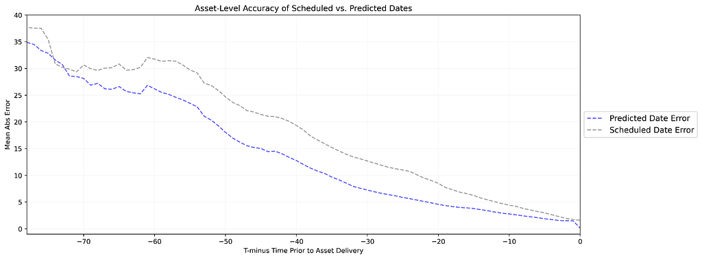
Figure 3. This plot compares accuracy (measured as Mean Absolute Error) between predicted and scheduled dates. The horizontal axis plots time prior to delivery, which decreases from left to right until you reach the moment of delivery at the bottom right. For this particular asset, the predicted delivery dates on average are much more accurate than manually scheduled delivery dates throughout the full horizon to delivery.

Since our teams use these dates over a period of time and not at a single point in time, there is an additional benefit that we’re describing as an Earlier Accuracy Signal. By leveraging predictive dates, our teams benefit from a level of accuracy that they would otherwise have to wait x amount of time for if using scheduled dates. As an example, 6 months out from Locked Cut delivery the predicted dates are better than scheduled dates on 76% of titles and have a level of accuracy (6.1 wks MAE) that scheduled dates don’t reach until 11 weeks later.

Circling back to AED, which we mentioned earlier is correlated to launch misses, we find that in our backtested titles globally, and across most buying orgs and content types (i.e., series versus standalones), predicted IMF and Locked Cut dates reduce AED from scheduled dates when calculated across the 6 months leading up to delivery. We see similar patterns when we repeat this for shorter horizons to delivery as well.

Streamlining Workflows with Improved Scheduling

A key advantage of this predictive model is that estimated delivery dates are already integral to our stakeholders’ workflows — meaning we can introduce predictive dates without overhauling existing processes. However, this creates a new challenge: with both scheduled and predicted dates available, teams need to determine which is more reliable. While predictive dates are often more accurate on average, there are situations where scheduled dates perform better. To address this, we’ve built serving logic that defaults to scheduled dates in buying orgs where the model underperforms. Elsewhere, teams can view both dates side by side in dashboards, allowing them to apply their own judgment. Additionally, our predictive models leverage features that are tied to scheduled dates, which has emphasized the need and impact of ensuring our upstream teams continue to input and update scheduled dates even in the presence of our predictions. We’re piloting these predictive signals in multiple ways, tailoring the approach to fit the diverse needs and tools of our various launch prep functions.


Predicting Risk in Content Launches: How Data-Driven Insights can Transform Launch Planning was originally published in Netflix TechBlog on Medium, where people are continuing the conversation by highlighting and responding to this story.

Fixing Performance Regressions Before they Happen

Post Syndicated from Netflix Technology Blog original https://netflixtechblog.com/fixing-performance-regressions-before-they-happen-eab2602b86fe

Angus Croll

Netflix is used by 222 million members and runs on over 1700 device types ranging from state-of-the-art smart TVs to low-cost mobile devices.

At Netflix we’re proud of our reliability and we want to keep it that way. To that end, it’s important that we prevent significant performance regressions from reaching the production app. Sluggish scrolling or late rendering is frustrating and triggers accidental navigations. Choppy playback makes watching a show less enjoyable. Any performance regression that makes it into a product release will degrade user experience, so the challenge is to detect and fix such regressions before they ship.

This post describes how the Netflix TVUI team implemented a robust strategy to quickly and easily detect performance anomalies before they are released — and often before they are even committed to the codebase.

What do we mean by Performance?

Technically, “performance” metrics are those relating to the responsiveness or latency of the app, including start up time.

But TV devices also tend to be more memory constrained than other devices, and as such are more liable to crash during a memory spike — so for Netflix TV we actually care about memory at least as much as performance, maybe more so.

At Netflix the term “performance” usually encompasses both performance metrics (in the strict meaning) and memory metrics, and that’s how we’re using the term here.

Why do we run Performance Tests on commits?

It’s harder to reason about the performance profile of pre-production code since we can’t gather real-time metrics for code that hasn’t yet shipped. We do cut a canary release in advance of shipment which is dogfooded by Netflix employees and subject to the same metrics collection as the production release. While the canary release is a useful dry-run for pending shipments, it sometimes misses regressions because the canary user base is a fraction of the production release. And in the event that regressions are detected in the canary, it still necessitates an often messy and time consuming revert or patch.

By running performance tests against every commit (pre- and post-merge), we can detect potentially regressive commits earlier. The sooner we detect such commits the fewer subsequent builds are affected and the easier it is to revert. Ideally we catch regressions before they even reach the main branch.

What are the Performance Tests?

The goal of our TVUI Performance Tests is to gather memory and responsiveness metrics while simulating the full range of member interactions with Netflix TV.

There are roughly 50 performance tests, each one designed to reproduce an aspect of member engagement. The goal is to keep each test brief and focused on a specific, isolated piece of functionality (startup, profile switching, scrolling through titles, selecting an episode, playback etc.), while the test suite as a whole should cover the entire member experience with minimal duplication. In this way we can run multiple tests in parallel and the absence of long pole tests keeps the overall test time manageable and allows for repeat test runs. Every test runs on a combination of devices (physical and virtual) and platform versions (SDKs). We’ll refer to each unique test/device/SDK combination as a test variation.

We run the full performance suite twice per Pull Request (PR):

  • when the PR is first submitted
  • when the PR is merged to the destination branch

Measurement

Each performance test tracks either memory or responsiveness. Both of these metrics will fluctuate over the course of a test, so we post metric values at regular intervals throughout the test. To compare test runs we need a method to consolidate this range of observed values into a single value.

We made the following decisions:

Memory Tests: use the maximum memory value observed during the test run (because that’s the value that determines whether a device could crash).

Responsiveness Tests : use the median value observed during the test run (based on the assumption that perceived slowness is influenced by all responses, not just the worst response).

What are the Challenges?

When Netflix is running in production, we capture real-time performance data which makes it relatively easy to make assertions about the app’s performance. It’s much harder to assess the performance of pre-production code (changes merged to the main branch but not yet released) and harder still to get a performance signal for unmerged code in a PR. Performance test metrics are inferior to real-time usage metrics for several reasons:

  • Data volume: In the Netflix app, the same steps are repeated billions of times, but developer velocity and resource constraints dictate that performance tests can only run a handful of times per build.
  • Simulation: No matter how rigorous or creative our testing process is, we can only ever approximate the experience of real life users, never replicate it. Real users regularly use Netflix for hours at a time, and every user has different preferences and habits.
  • Noise: Ideally a given codebase running any given test variation will always return identical results. In reality that just never happens: no two device CPUs are identical, garbage collection is not entirely predictable, API request volume and backend activity is variable — so are power levels and network bandwidth. For every test there will be background noise that we need to somehow filter from our analysis.

Initial Approach: Static Thresholds

For our first attempt at performance validation we assigned maximum acceptable threshold values for memory metrics. There was a sound rationale behind this approach — when a TV runs Netflix there is a hard limit for memory footprint beyond which Netflix has the potential to crash.

There were several issues with the static thresholds approach:

  • Custom preparation work per test: Since each test variation has a unique memory profile, the appropriate static threshold had to be researched and assigned on a case-by-case basis. This was difficult and time consuming, so we only assigned thresholds to about 30% of test variations.
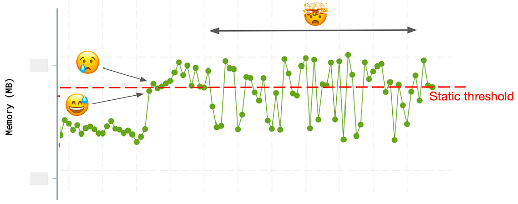
  • Lack of context: As a validation technique, static thresholds proved to be somewhat arbitrary. Imagine a commit that increases memory usage by 10% but to a level which is just below the threshold. The next commit might be a README change (zero memory impact) but due to normal variations in device background noise, the metric could increase by just enough to breach the threshold.
  • Background variance is not filtered: Once the codebase is bumping against the memory threshold, background device noise becomes the principal factor determining which side of the threshold line the test result falls.
Unreliable regression signals with static Threshold technique
  • Post-alert adjustments: We found ourselves repeatedly increasing the thresholds to move them clear of background noise

The Pivot: Anomaly and Changepoint Detection

It became apparent we needed a technique for performance validation that:

  • Removes failure bias by giving equal weight to all test runs, regardless of results
  • Doesn’t treat performance data points in isolation, but instead assesses the performance impact of a build in relation to previous builds.
  • Can be automatically applied to every test without the need for pre-hoc research, data entry or ongoing manual intervention
  • Could be equally applied to test data of any type: memory, responsiveness, or any other non-boolean test data
  • Minimizes the impact of background noise by prioritizing variance over absolute values
  • Improves insight by examining data points both at the time of creation and retroactively

We settled on a two-pronged approach:

  • Anomaly Detection immediately calls out potential performance regressions by comparing with recent past data
  • Changepoint Detection identifies more subtle performance inflections by examining past and future data clusters

Anomaly Detection

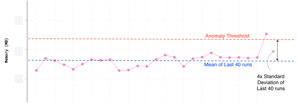
We define an anomaly as any metric data point that is more than n standard deviations above the recent mean, where recent mean and standard deviation are derived from the previous m test runs. For Netflix TV performance tests we currently set n to 4 and m to 40 but these values can be tweaked to maximize signal to noise ratio. When an anomaly is detected the test status is set to failed and an alert is generated.

Anomaly detection works because thresholds are dynamic and derived from existing data. If the data exhibits a lot of background variance then the anomaly threshold will increase to account for the extra noise.

Changepoints

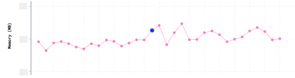
Changepoints are data points at the boundary of two distinct data distribution patterns. We use a technique called e-divisive to analyze the 100 most recent test runs, using a Python implementation based on this implementation.

Since we’re only interested in performance regressions, we ignore changepoints that trend lower. When a changepoint is detected for a test, we don’t fail the test or generate an alert (we consider changepoints to be warnings of unusual patterns, not full blown error assertions).

As you can see, changepoints are a more subtle signal. They don’t necessarily indicate a regression but they suggest builds that had an impact on subsequent data distribution.

Builds that generate changepoints across multiple tests, warrant further investigation before they can be included in the release candidate.

Changepoints give us more confidence in regression detection because they disregard false positives such as one time data spikes. Because changepoint detection requires after-the-fact data, they are best suited to identifying potentially regressive code that is already in the main branch but has not yet been shipped.

Additional Adjustments

Runs per Test

To address failure bias, we decided to run all tests 3 times, regardless of the result. We chose 3 iterations to provide enough data to eliminate most device noise (tests are allocated to devices randomly) without creating a productivity bottleneck.

Summarizing across Test Runs

Next we needed to decide on a methodology to compress the results of each batch of 3 runs into a single value. The goal was to ignore outlier results caused by erratic device behavior.

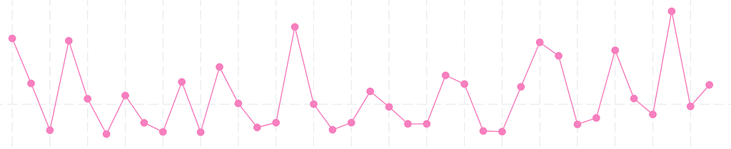
Initially we took the average of those three runs, but that led to an excess of false positives because the most irregular test runs exerted too much influence on the result. Switching to the median eliminated some of these false positives but we were still getting an unacceptable number of excess alerts (because during periods of high device noise we would occasionally see outlier results two times out of three). Finally, since we noticed that outlier results tended to be higher than normal — rarely lower — we settled on using the minimum value across the 3 runs and this proved to be the most effective at eliminating external noise.

All data points (3 runs per build)
Selecting median value per build
Selecting minimum value per build

What were the Results?

After switching our performance validation to use anomaly and changepoint detection we noticed several improvements.

a) We are alerted for potential performance regressions far less often, and when we do get alerted it’s much more likely to indicate a genuine regression. Our workload is further reduced by no longer having to manually increment static performance thresholds after each false positive.

The following table represents the alert summary for two distinct months last year. In March 2021 we still used static thresholds for regression alerts. By October 2021 we had switched using anomaly detection for regression alerts. Alerts which were true regressions is the number of alerted commits for which the suspected regression turned out to be both significant and persistent.

Note that since the March tests only validated when a threshold was manually set, the total number of validating test runs in October was much greater, and yet we still got only 10% of the alerts.

b) We are not alerted for subsequent innocuous builds that inherit regressive commits from preceding builds. (Using the static threshold technique, all subsequent builds were alerted until the regressive build was reverted.) This is because regressive builds increase both mean and standard deviation and thus put subsequent non-regressing builds comfortably below the alert threshold.

Regressive build is above alert threshold
Subsequent build is easily below alert threshold

c) Performance tests against PRs, which had been almost constantly red (because the probability of at least one static threshold being breached was always high), are now mostly green. When the performance tests are red we have a much higher confidence that there is a genuine performance regression.

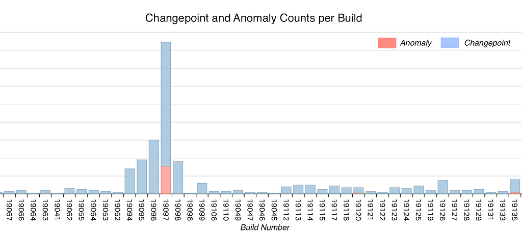
d) Displaying the anomaly and changepoint count per build provides a visual snapshot that quickly highlights potentially problematic builds.

What’s Next?

Further Work

There are still several things we’d like to improve

  • Make it easier to determine if regressions were due to external agents: Often it turns out the detected regression, though real, was not a result of the committed code but due to an external factor such as an upgrade to one of our platform dependencies, or a feature flag that got switched on. It would be helpful to summarize external changes in our alert summaries.
  • Factor out resolved regressions when determining baselines for validation:
    When generating recent mean and standard deviation values, we could improve regression detection by filtering out data from erstwhile regressions that have since been fixed.
  • Improve Developer Velocity: We can further reduce total test time by removing unnecessary iterations within tests, adding more devices to ensure availability, and de-emphasizing testing for those parts of the app where performance is less likely to be critical. We can also pre-build app bundles (at least partially) so that the test suite is not delayed by waiting for fresh builds.
  • More closely mirror metrics gathered by the production app: In the deployed Netflix TV app we collect additional metrics such as TTR (time to render) and empty box rate (how frequently titles in the viewport are missing images). While test metrics and metrics collected during real use do not lend themselves to direct comparison, measuring the relative change in metrics in pre-production builds can help us to anticipate regressions in production.

Wider Adoption and New Use Cases

At this point Anomaly and Changepoint detection is applied to every commit in the TVUI repo, and is in the process of being deployed for commits to the TV Player repo (the layer that manages playback operations). Other Netflix teams (outside of the TV platform) have also expressed interest in these techniques and the ultimate goal is to standardize regression detection across Netflix.

Anomaly and changepoint detection are entirely framework independent — the only required inputs are a current value and an array of recent values to compare it to. As such, their utility extends far beyond performance tests. For example, we are considering using these techniques to monitor the reliability of non-performance-based test suites — in this case the metric of interest is the percent of tests that ran to completion.

In the future we plan to decouple anomaly and changepoint logic from our test infrastructure and offer it as a standalone open-source library.

Wrap Up

By using techniques that assess the performance impact of a build in relation to the performance characteristics (magnitude, variance, trend) of adjacent builds, we can more confidently distinguish genuine regressions from metrics that are elevated for other reasons (e.g. inherited code, regressions in previous builds or one-off data spikes due to test irregularities). We also spend less time chasing false negatives and no longer need to manually assign a threshold to each result — the data itself now sets the thresholds dynamically.

This improved efficiency and higher confidence level helps us to quickly identify and fix regressions before they reach our members.

The anomaly and changepoint techniques discussed here can be used to identify regressions (or progressions), unexpected values or inflection points in any chronologically sequenced, quantitative data. Their utility extends well beyond performance analysis. For example they could be used to identify inflection points in system reliability, customer satisfaction, product usage, download volume or revenue.

We encourage you to try these techniques on your own data. We’d love to learn more about their success (or otherwise) in other contexts!


Fixing Performance Regressions Before they Happen was originally published in Netflix TechBlog on Medium, where people are continuing the conversation by highlighting and responding to this story.