Post Syndicated from Siddharth Thacker original https://aws.amazon.com/blogs/big-data/how-aruba-networks-built-a-cost-analysis-solution-using-aws-glue-amazon-redshift-and-amazon-quicksight/

This is a guest post co-written by Siddharth Thacker and Swatishree Sahu from Aruba Networks.

Aruba Networks is a Silicon Valley company based in Santa Clara that was founded in 2002 by Keerti Melkote and Pankaj Manglik. Aruba is the industry leader in wired, wireless, and network security solutions. Hewlett-Packard acquired Aruba in 2015, making it a wireless networking subsidiary with a wide range of next-generation network access solutions.

Aruba Networks provides cloud-based platform called Aruba Central for network management and AI Ops. Aruba cloud platform supports thousands of workloads to support customer facing production environment and also a separate development platform for Aruba engineering.

The motivation to build the solution presented in this post was to understand the unit economics of the AWS resources used by multiple product lines across different organization pillars. Aruba wanted a faster, effective, and reliable way to analyze cost and usage data and visualize that into a dashboard. This solution has helped Aruba in multiple ways, including:

• Visibility into costs – Multiple Aruba teams can now analyze the cost of their application via data surfaced with this solution
• Cost optimization – The solution helps teams identify new cost-optimization opportunities by making them aware of the higher-cost resources with low utilization so they can optimize accordingly
• Cost management – The Cloud DevOps organization, the group who built this solution, can effectively plan at the application level and have a direct positive impact on gross margins
• Cost savings – With daily cost data available, engineers can see the monetary impact of right-sizing compute and other AWS resources almost immediately
• Big picture as well as granular – Users can visualize cost data from the top down and track cost at a business level and a specific resource level

Overview of the solution

This post describes how Aruba Networks automated the solution, from generating the AWS Cost & Usage Report (AWS CUR) to its final visualization on Amazon QuickSight. In this solution, they start by configuring the CUR on their primary payer account, which publishes the billing reports to an Amazon Simple Storage Service (Amazon S3) bucket. Then they use an AWS Glue crawler to define and catalog the CUR data. As the new CUR data is delivered daily, the data catalog is updated, and the data is loaded into an Amazon Redshift database using Amazon Redshift Spectrum and SQL. The reporting and visualization layer is built using QuickSight. Finally, the entire pipeline is automated by using AWS Data Pipeline.

The following diagram illustrates this architecture.

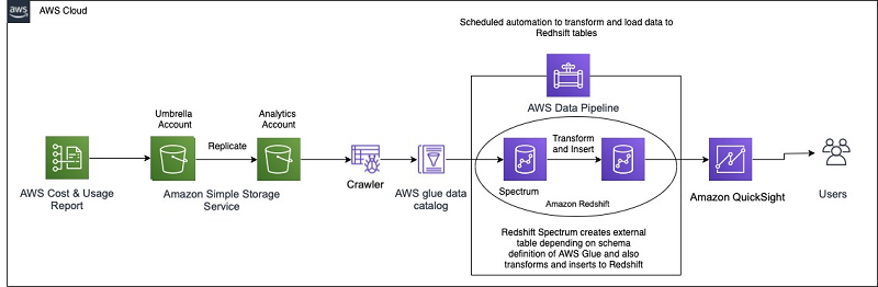
Aruba prefers the AWS CUR Report to AWS Cost Explorer because AWS Cost Explorer provides usage information at a high level, and not enough granularity for detailed operations, such as data transfer cost. AWS CUR provides the most detailed information available about your AWS costs and usage at an hourly granularity. This allows the Aruba team to drill down the costs by the hour or day, product or product resource, or custom tags, enabling them to achieve their goals.

Aruba implemented the solution with the following steps:

1. Set up the CUR delivery to a primary S3 bucket from the billing dashboard.
2. Use Amazon S3 replication to copy the primary payer S3 bucket to the analytics bucket. Having a separate analytics account helps prevent direct access to the primary account.
3. Create and schedule the crawler to crawl the CUR data. This is required to make the metadata available in the Data Catalog and update it quickly when new data arrives.
4. Create respective Amazon Redshift schema and tables.
5. Orchestrate an ETL flow to load data to Amazon Redshift using Data Pipeline.
6. Create and publish dashboards using QuickSight for executives and stakeholders.

Insights generated

The Aruba DevOps team built various reports that provide the cost classifications on AWS services, weekly cost by applications, cost by product, infrastructure, resource type, and much more using the detailed CUR data as shown by the following screenshot.

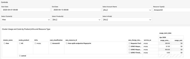
For example, using the following screenshot, Aruba can conveniently figure out that compute cost is the biggest contributor compared to other costs. To reduce the cost, they can consider using various cost-optimization methods like buying reserved instances, savings plans, or Spot Instances wherever applicable.

Similarly, the following screenshot highlights the cost doubled compared to the first week of April. This helps Aruba to identify anomalies quickly and make informed decisions.

Setting up the CUR delivery

For instructions on setting up a CUR, see Creating Cost and Usage Reports.

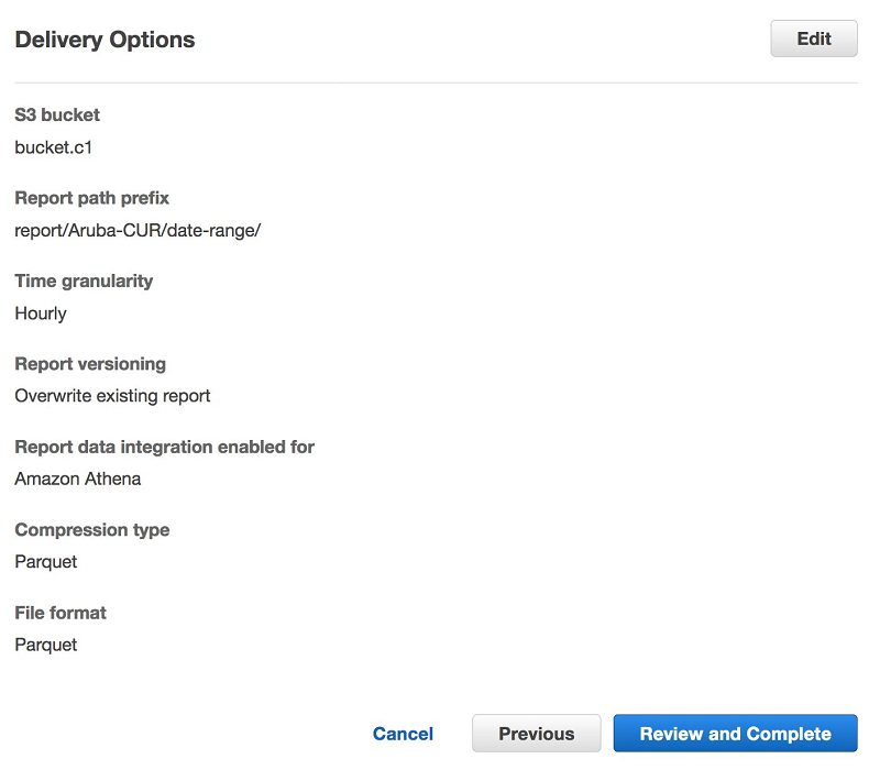
To reduce complexity in the workflow, Aruba chose to create resources in the same region with hourly granularity, mainly to see metrics more frequently.

To lower the storage costs for data files and maximize the effectiveness of querying data with serverless technologies like Amazon Athena, Amazon Redshift Spectrum, and Amazon S3 data lake, save the CUR in Parquet format. The following screenshot shows the configuration for delivery options.

The following table shows some example CUR data.

Replicating the CUR data to your analytics account

For security purposes, other teams aren’t allowed to access the primary (payer) account, and therefore can’t access CUR data generated from that account. Aruba replicated the data to their analytics account and build the cost analysis solution there. Other teams can access the cost data without getting access permission for the primary account. The data is replicated across accounts by adding an Amazon S3 replication rule in the bucket. For more information, see Adding a replication rule when the destination bucket is in a different AWS account.

Cataloging the data with a crawler and scheduling it to run daily

Because AWS delivers all daily reports in a report date range report-prefix/report-name/yyyymmdd-yyyymmdd folder, Aruba uses AWS Glue crawlers to crawl through the data and update the catalog.

AWS Glue is a fully managed ETL service that makes it easy to prepare and load the data for analytics. Once the AWS Glue is pointed to the data stored on AWS, it discovers the data and stores the associated metadata (such as table definition and schema) in the Data Catalog. After the data is cataloged, the data is immediately searchable, queryable, and available for ETL. For more information, see Populating the AWS Glue Data Catalog.

The following screenshot shows the crawler created on Amazon S3 location of the CUR data.

The following code is an example table definition populated by the crawler.:

CREATE EXTERNAL TABLE `cur_parquet`(
  `identity_line_item_id` string, 
  `identity_time_interval` string, 
  `bill_invoice_id` string, 
………
………
  `resource_tags_user_infra_role` string)

PARTITIONED BY ( 
  `year` string, 
  `month` string )

ROW FORMAT SERDE  'org.apache.hadoop.hive.ql.io.parquet.serde.ParquetHiveSerDe'
STORED AS INPUTFORMAT   'org.apache.hadoop.hive.ql.io.parquet.MapredParquetInputFormat' 
OUTPUTFORMAT   'org.apache.hadoop.hive.ql.io.parquet.MapredParquetOutputFormat'
LOCATION
  's3://curS3bucket/Parquet/'

Transforming and loading using Amazon Redshift

Next in the analytics service, Aruba chose Amazon Redshift over Athena. Aruba has a use case to integrate cost data together with other tables already present in Amazon Redshift and hence using the same service makes it easy to integrate with their existing data. To further filter and transform data at the same time, and simplify the multi-step ETL, Aruba chose Amazon Redshift Spectrum. It helps to efficiently query and load CUR data from Amazon S3. For more information, see Getting started with Amazon Redshift Spectrum.

Use the following query to create an external schema and map it to the AWS Glue database created earlier in the Data Catalog:

--Choose a schema name of your choice, cur_redshift_external_schema name is just an example--
 create external schema cur_redshift_spectrum_external_schema from data catalog database 
 'aruba_curr_db' iam_role 'arn:aws:iam::xxxxxxxxxxxxx:role/redshiftclusterrole' 
 create external database if not exists;

The table created in the Data Catalog appears under the Amazon Redshift Spectrum schema. The schema, table, and records created can be verified with the following SQL code:

SELECT Count(*) 
FROM   cur_redshift_spectrum_external_schema.<TABLE>; 

--Query the right partition, year=2020 and month=2 is used an example
SELECT Count(*) 
FROM   cur_redshift_spectrum_external_schema.<TABLE> 
WHERE  year=2020 
AND    month=2;

Next, transform and load the data into the Amazon Redshift table. Aruba started by creating an Amazon Redshift table to contain the data. The following SQL code can be used to create the production table with the desired columns:

CREATE TABLE redshift_schema.redshift_table 
  ( 
     usage_start_date TIMESTAMP, 
     usage_end_date   TIMESTAMP, 
     service_region   VARCHAR (256), 
     service_az       VARCHAR (256), 
     aws_resource_id  VARCHAR (256), 
     usage_amount     FLOAT (17), 
     charge_currency  VARCHAR (256), 
     aws_product_name VARCHAR (256), 
     instance_family  VARCHAR (256), 
     instance_type    VARCHAR (256), 
     unblended_cost   FLOAT (17), 
     usage_cost       FLOAT (17)
  ); 

CUR is dynamic in nature, which means that some columns may appear or disappear with each update. When creating the table, we take static columns only. For more information, see Line item details.

Next, insert and update to ingest the data from Amazon S3 to the Amazon Redshift table. Each CUR update is cumulative, which means that each version of the CUR includes all the line items and information from the previous version.

The reports generated throughout the month are estimated and subject to change during the rest of the month. AWS finalizes the report at the end of each month. Finalized reports have the calculations for the blended and unblended costs, and cover all the usage for the month. For this use case, Aruba updates the last 45 days of data to make sure the finalized cost is captured. The below sample query can be used to verify the updated data:

-- Create Table Statement
 INSERT INTO redshift_schema.redshift_table
            (usage_start_date, 
             usage_end_date, 
             service_region, 
             service_az, 
             aws_resource_id, 
             usage_amount, 
             charge_currency, 
             aws_product_name, 
             instance_family, 
             instance_type, 
             unblended_cost,
             Usage_Cost ) 
 SELECT line_item_usage_start_date, 
       line_item_usage_end_date, 
       line_item_operation, 
       line_item_availability_zone, 
       line_item_resource_id, 
       line_item_usage_amount, 
       line_item_currency_code, 
       product_product_name, 
       product_instance_family, 
       product_instance_type, 
       line_item_unblended_cost,
       case when line_item_type='Usage' then line_item_unblended_cost
            else 0
            end as usage_cost 
 FROM   cur_redshift_external_schema.cur_parquet_parquet
 WHERE  line_item_usage_start_date >= date_add('day', -45, getdate()) 
       AND line_item_usage_start_date < date_add('day', 1, getdate()); 

Using Data Pipeline to orchestrate the ETL workflow

To automate this ETL workflow, Aruba chose Data Pipeline. Data Pipeline helps to reliably process and move data between different AWS compute and storage services, as well as on-premises data sources. With Data Pipeline, Aruba can regularly access their data where it’s stored, transform and process it at scale, and efficiently transfer the results to AWS services such as Amazon S3, Amazon Relational Database Service (Amazon RDS), Amazon DynamoDB, and Amazon EMR. Although the detailed steps of setting up this pipeline are out of scope for this blog, there is a sample workflow definition JSON file, which can be imported after making the necessary changes.

Data Pipeline workflow

The following screenshot shows the multi-step ETL workflow using Data Pipeline. Data Pipeline is used to run the INSERT query daily, which inserts and updates the latest CUR data into our Amazon Redshift table from the external table.

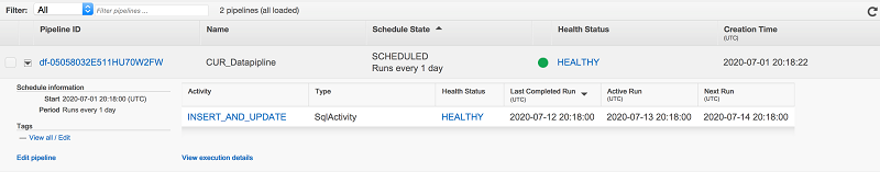
In order to copy data to Amazon Redshift,  RedshiftDataNode and RedshiftCopyActivity can be used, and then scheduled to run periodically.

Sharing metrics and creating visuals with QuickSight

To share the cost and usage with other teams, Aruba choose QuickSight using Amazon Redshift as the data source. QuickSight is a native AWS service that seamlessly integrates with other AWS services such as Amazon Redshift, Athena, Amazon S3, and many other data sources.

As a fully managed service, QuickSight lets Aruba to easily create and publish interactive dashboards that include ML Insights. In addition to building powerful visualizations, QuickSight provides data preparation tools that makes it easy to filter and transform the data into the exact needed dataset. As a cloud-native service, dashboards can be accessed from any device and embedded into applications and portals, allowing other teams to monitor their resource usage easily. For more information about creating a dataset, see Creating a Dataset from a Database. Quicksight Visuals can then be created from this dataset.

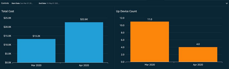
The following screenshot shows a visual comparison of device cost and count to help find the cost per device. This visual helped Aruba quickly identify the cost per device increase in April and take necessary actions.

Similarly, the following visualization helped Aruba identify an increase in data transfer cost and helped them decide to invest in rearchitecting their application.

The following visualization classifies the cost spend per resource.

Conclusion

In this post, we discussed how Aruba Networks was able to successfully achieve the following:

• Generate CUR and use AWS Glue to define data, catalog the data, and update the metadata
• Use Amazon Redshift Spectrum to transform and load the data to Amazon Redshift tables
• Query, visualize, and share the data stored using QuickSight
• Automate and orchestrate the entire solution using Data Pipeline

Aruba use this solution to automatically generate a daily cost report and share it with their stakeholders, including executives and cloud operations team.

About the Authors

Siddharth Thacker works in Business & Finance Strategy in Cloud Software division at Aruba Networks. Siddharth has Master’s in Finance with experience in industries like banking, investment management, cloud software and focuses on business analytics, margin improvement and strategic partnerships at Aruba. In his spare time, he likes exploring outdoors and participate in team sports.

Swatishree Sahu is a Technical Data Analyst at Aruba Networks. She has lived and worked in India for 7 years as an SME for SOA-based integration tools before coming to US to pursue her master’s in Business Analytics from UT Dallas. Breaking down and analyzing data is her passion. She is a Star Wars geek, and in her free time, she loves gardening, painting, and traveling.

Ritesh Chaman is a Technical Account Manager at Amazon Web Services. With 10 years of experience in the IT industry, Ritesh has a strong background in Data Analytics, Data Management, and Big Data systems. In his spare time, he loves cooking (spicy Indian food), watching sci-fi movies, and playing sports.

Kunal Ghosh is a Solutions Architect at AWS. His passion is to build efficient and effective solutions on the cloud, especially involving Analytics, AI, Data Science, and Machine Learning. Besides family time, he likes reading and watching movies, and is a foodie.