Managing database environments demands a balance of resource efficiency and scalability. Organizations need flexible options across their entire database lifecycle, spanning development, testing, and production workloads with diverse storage and compute requirements.
To address these needs, we’re announcing four new capabilities for Amazon Relational Database Service (Amazon RDS) to help customers optimize their costs as well as improve efficiency and scalability for their Amazon RDS for Oracle and Amazon RDS for SQL Server databases. These enhancements include SQL Server Developer Edition support and expanded storage capabilities for both RDS for Oracle and RDS for SQL Server. Additionally, you can have CPU optimization options for RDS for SQL Server on M7i and R7i instances, which offer price reductions from previous generation instances and separately billed licensing fees.
Let’s explore what’s new.
SQL Server Developer Edition support SQL Server Developer Edition is now available on RDS for SQL Server, offering a free SQL Server edition that includes all the Enterprise Edition functionalities. Developer Edition is licensed specifically for non-production workloads, so you can build and test applications without incurring SQL Server licensing costs in your development and testing environments.
This release brings significant cost savings to your development and testing environments, while maintaining consistency with your production configurations. You’ll have access to all Enterprise Edition features in your development environment, making it easier to test and validate your applications. Additionally, you’ll benefit from the full suite of Amazon RDS features, including automated backups, software updates, monitoring, and encryption capabilities throughout your development process.
To get started, upload your SQL Server binary files to Amazon Simple Storage Service (Amazon S3) and use them to create your Developer Edition instance. You can migrate existing data from your Enterprise or Standard Edition instances to Developer Edition instances using built-in SQL Server backup and restore operations.
M7i/R7i instances on RDS for SQL Server with support for optimize CPU You can now use M7i and R7i instances on Amazon RDS for SQL Server to achieve several key benefits. These instances offer significant cost savings over previous generation instances. You also get improved transparency over your database costs with licensing fees and Amazon RDS DB instances costs billed separately.
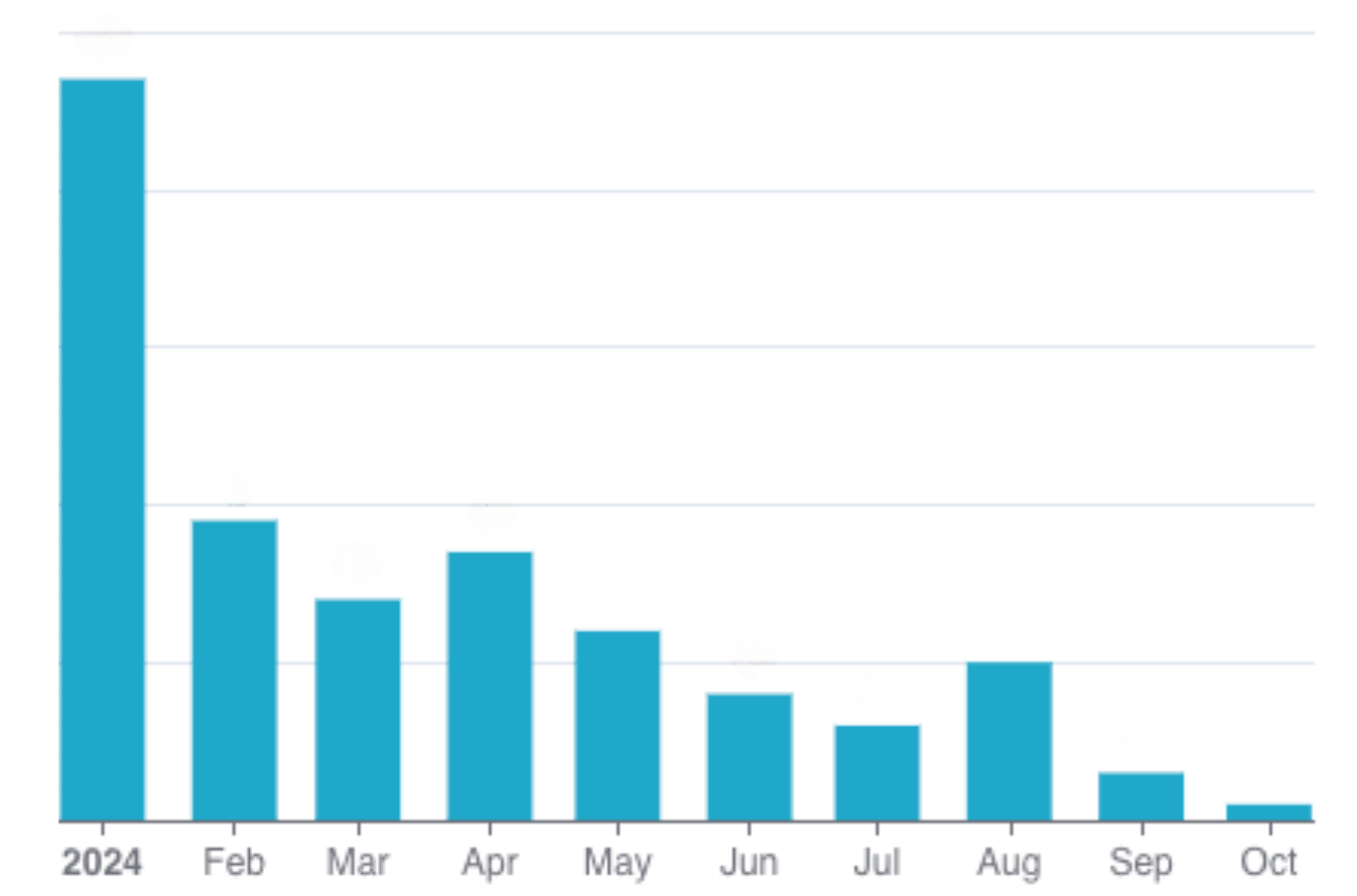
RDS for SQL Server M7i/R7i instances offer up to 55% lower costs compared to previous generation instances.
Using the optimize CPU capability on these instances, you can customize the number of vCPUs on license-included RDS for SQL Server instances. This enhancement is particularly valuable for database workloads that require high memory and input/output operations per second (IOPS), but lower vCPU counts
This feature provides substantial benefits for your database operations. You can significantly reduce vCPU-based licensing costs while maintaining the same memory and IOPS performance levels your applications require. The capability supports higher memory-to-vCPU ratios and automatically disables hyperthreading while maintaining instance performance. Most importantly, you can fine-tune your CPU settings to precisely match your specific workload requirements, providing optimal resource utilization.
To get started, select SQL Server with an M7i or R7i instance type when creating a new database instance. Under Optimize CPU select Configure the number of vCPUs and set your desired vCPU count.
Additional storage volumes for RDS for Oracle and SQL Server Amazon RDS for Oracle and Amazon RDS for SQL Server now support up to 256 TiB storage size, a fourfold increase in storage size per database instance, through the addition of up to three additional storage volumes.
The additional storage volumes provide extensive flexibility in managing your database storage needs. You can configure your volumes using both io2 and gp3 volumes to create an optimal storage strategy. You can store frequently accessed data on high-performance Provisioned IOPS SSD (io2) volumes while keeping historical data on cost-effective General Purpose SSD (gp3) volumes, which balances performance and cost. For temporary storage needs, such as month-end processing or data imports, you can add storage volumes as needed. After these operations are complete, you can empty the volumes and then remove them to reduce unnecessary storage costs.
These storage volumes offer operational flexibility with zero downtime and you can add or remove additional storage volumes without interrupting your database operations. You can also scale up multiple volumes in parallel to quickly meet growing storage demands. For Multi-AZ deployments, all additional storage volumes are automatically replicated to maintain high availability.
Let me show you a quick example. I’ll add a storage volume to an existing RDS for Oracle database instance.
First, I navigate to the RDS console, then to my RDS for Oracle database instance detail page. I look under Configuration and I find the Additional storage volumes section.
You can add up to three additional storage volumes and each must be named according to a naming convention. Storage volumes can’t have the same name and you must choose between rdsdbdata2, rdsdbdata3, and rdsdbdata4. For RDS for Oracle database instances, I can add additional storage volumes to the database instance with the primary storage volume size of 200 GiB or higher.
I’m going to add two volumes, so I choose Add additional storage volume and then fill in all the required information. I choose rdsdbdata2 as the volume name and give it 12000 GiB of allocated storage with 60000 provisioned IOPS on an io2 storage type. For my second additional storage volume, rdsdbdata3, I choose to have 2000 GiB on gp3 with 15000 provisioned IOPS.
After confirmation, I wait for Amazon RDS to process my request and then my additional volumes are available.
You can also use the AWS CLI to add volumes during creation of database instances or when modifying them.
Things to know These capabilities are now available in all commercial AWS Regions and the AWS GovCloud (US) Regions where Amazon RDS for Oracle and Amazon RDS for SQL Server are offered.
Since Amazon Web Services (AWS) introduced Savings Plans, customers have been able to lower the cost of running sustained workloads while maintaining the flexibility to manage usage across accounts, resource types, and AWS Regions. Today, we’re extending this flexible pricing model to AWS managed database services with the launch of Database Savings Plans, which help customers reduce database costs by up to 35% when they commit to a consistent amount of usage ($/hour) over a 1-year term. Savings automatically apply each hour to eligible usage across supported database services, and any additional usage beyond the commitment is billed at on-demand rates.
As organizations build and manage data-driven and AI applications, they often use different database services, engines and deployment types, including instance-based and serverless options, to meet evolving business needs. Database Savings Plans provide the flexibility to choose how workloads run while maintaining cost efficiency. If customers are in the middle of a migration or modernization effort, they can switch database engines and adjust deployment types, such as from provisioned to serverless as part of ongoing cost optimization, while continuing to receive discounted rates. If a customer’s business expands globally, they can also shift usage across AWS Regions and continue to benefit from the same commitment. By applying a consistent hourly commitment, customers can maintain predictable spend even as usage patterns evolve and analyze coverage and utilization using familiar cost management tools.
New Savings Plans Each plan defines where pricing applies, the range of available discounts, and the level of flexibility provided across supported database engines, instance families, sizes, deployment options, or AWS Regions.
Discounts vary by deployment model and service type. Serverless deployments provide up to 35% savings compared to on-demand rates. Provisioned instances across supported database services deliver up to 20% savings. For Amazon DynamoDB and Amazon Keyspaces, on-demand throughput workloads receive up to 18% savings, and provisioned capacity offers up to 12%. Together, these savings help customers optimize costs while maintaining consistent coverage for database usage. To learn more about the pricing and eligible usage, visit the Database Savings Plans pricing page.
Recommendations – are automatically generated from your recent on-demand usage. To reach the Recommendations view in the Billing and Cost Management console, choose Savings and Commitments, Savings Plans, and Recommendations in the navigation pane. In the Recommendations view, select Database Savings Plans and configure the Recommendation options. AWS Savings Plans recommendations analyze your historical on-demand usage to identify the hourly commitment that delivers the highest overall savings.
The Purchase Analyzer – is designed for modeling custom commitment levels. If you want to purchase a different amount than the recommended commitment on the Purchase Analyzer page, select Database Savings Plans and configure Lookback period and Hourly commitment to simulate alternative commitment levels and see the projected impact on Cost, Coverage, and Utilization.
This way is preferred if your purchasing strategy includes smaller, incremental commitments over time or if you expect future usage changes that could affect your ideal purchase amount.
After reviewing the recommendations or running simulations in Savings Plans Recommendations or Savings Plans Purchase Analyzer, choose Add to cart to proceed with your chosen commitment. If you prefer to purchase directly, you can also navigate to the Purchase Savings Plans page. The console updates estimated discounts and coverage in real time as you adjust each setting, so you can evaluate the impact before completing your order.
You can learn more about how to choose and purchase Database Saving Plans by visiting the Savings Plans User Guide documents.
Now available Database Savings Plans are available in all AWS Regions outside of China. Give them a try and start shaping your database strategy with more flexibility and predictable costs.
Ah, the familiar beep beep beep but don’t worry, it’s not your alarm coaxing you out of bed. No, this is far worse: the dreaded PagerDuty on-call alert! What’s the crisis this time? There appears to be an issue with high database CPU utilisation, overwhelmed by a flood of heavy traffic. If you’re a developer, chances are you’ve faced this scenario at least once. The very moment when you question every life decision while desperately searching for answers at 3 AM.
This article was born of one such heart-pounding, adrenaline-fuelled incident. Picture this: the database was struggling, the traffic was relentless, and the team was caught in the crossfire. The seemingly obvious solution was to migrate from SQL to NoSQL—a straightforward fix, or so it seemed. Instead of taking the easy way out, we stepped back, rolled up our sleeves, and tackled the problem head-on, embarking on a bold journey of optimisation.
What followed was a rollercoaster of trial, error, and a few “why did we even try this” moments. Yet, isn’t that the beauty of being a developer? Embracing the chaos, thriving in the madness, and eventually emerging victorious with a story worth sharing.
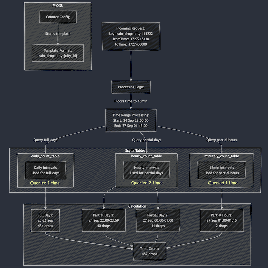
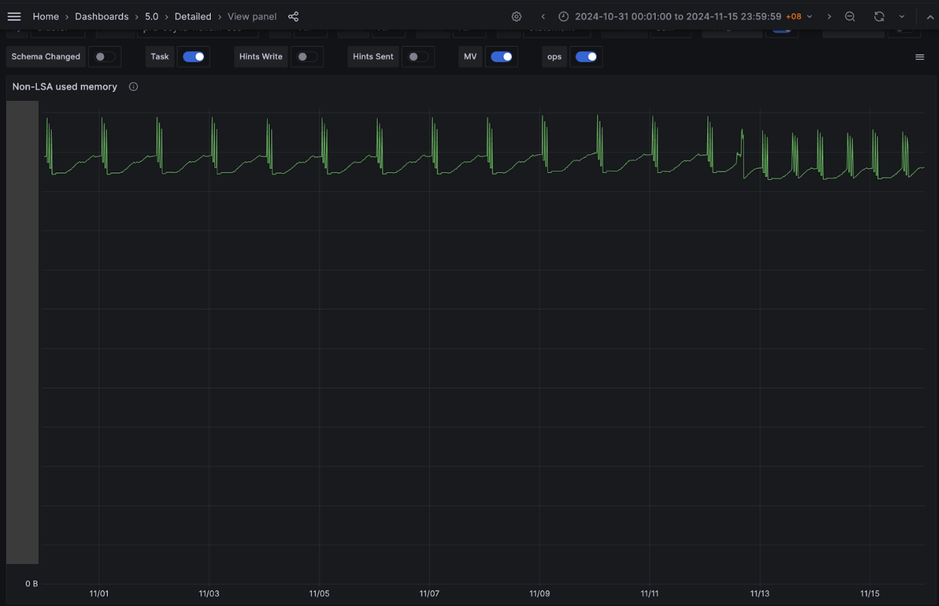
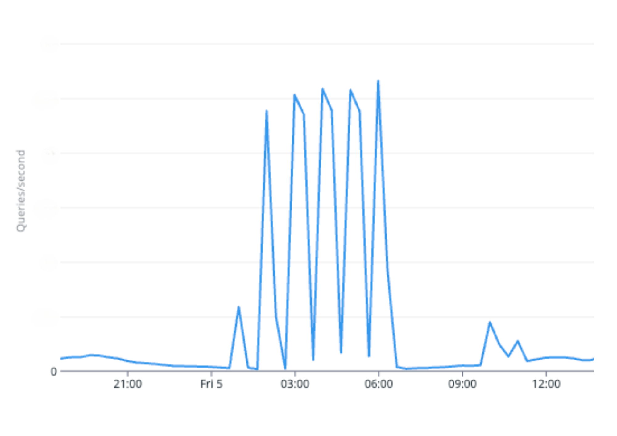
Real-time usage count tracking is a common use case that can be found across many applications, like Instagram’s post like count, YouTube’s watch count, or a marketing campaign usage count, which is used in monitoring and measuring the performance of marketing campaigns to assess effectiveness. These counts don’t have to be highly accurate, but rather an approximation in most use cases. This meant that in an occurrence of an event, instead of immediately updating the count in the database, the count is cached in the application server and later updated in batches to reduce the database Queries Per Second (QPS) and Central Processing Unit (CPU) utilisation.
This article shares one such use case where we optimised the campaign usage count tracking with highly concurrent in-memory caching that flushes to the database at periodic intervals.
Background
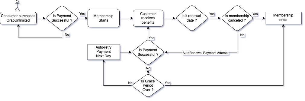
Marketing campaigns are configured to deliver push notifications, emails, and award rewards and points to Grab users. Total usage as well as daily usage needs to be tracked for display purposes to give a sense of how the campaign is performing. In this use case, accuracy is not a top priority. This release in constraint helps us to reduce write traffic by incrementing the counter in-memory and flushing the disk at periodic intervals for persistence.
In this section, let’s break down the process of designing a highly concurrent in-memory counter with data persistence.
Functional requirements
Upsert the counter value for the given key.
Periodically flush the counter value to the storage layer for persistence.
Non-functional requirements
Do note that although consistency is not critical for this use case, we will build a generic in-memory counter with the following guarantees, which can be reused for other use cases:
Highly consistent updates of the counter values in memory during high concurrency.
Consistent flushing of the counter values to the storage layer for persistence.
Simple GoLang code for writing an in-memory counter may look like the code sample shown in Figure 1.
Figure 1. In-memory counter code snippet.
The code has a map declared globally, and the do function increments the counter value against the key. However, this code fails to work when multiple Goroutines (GoLang version of threads) try to access this do function concurrently. This will result in the following error, as shown in Figure 2.
Figure 2. Code error sample.
Maps in GoLang are not thread safe and need to be locked when being accessed concurrently. The GoLang sync package has Mutex, which serves this locking purpose. The code changes are shown in Figure 3. The sync.RWMutex object is declared globally and every time the do function is called, the lock is obtained first. Then the map is mutated, followed by releasing the lock at the end. This code works as intended even when multiple go routines try to access it concurrently.
Figure 3. Implementing sync.RWMutex for locking purpose.
The code for the functional requirement of periodically flushing the counter value to the storage layer is shown in Figure 4.
Figure 4. Code snippet of flushing counter value to storage function.
Assuming that this design is a success, every 200 milliseconds, a background job acquires a global map lock, iterates over all keys, writes each entry to the storage layer asynchronously, then deletes it from the map. After that, a flush is executed where counter increments are blocked until the lock is released.
Can we do something better?
Yes, Sync.Map is the synchronised version of map in GoLang. This can be used to get rid of the explicit locking overheads.
Powerful features of the Sync.Map:
LoadOrStore: Retrieves the existing value for a key if present, or stores and returns a new value if the key is absent. Ensuring atomic operation and preventing race conditions.
CompareAndSwap: Atomically compares a variable’s current value to an expected value. If they match, it is swapped with a new value, ensuring thread-safe updates.
LoadAndDelete: Atomically retrieves and removes the value of a given key, returning the value and a boolean indicating if the key was present.
When combined, these Sync.Map features produce the do function shown in Figure 5. When the do function is called, the LoadOrStore function tries to atomically store the key in the map if the key is absent. Otherwise, it returns the current value for the key with the isLoaded variable set to true. If the key is already present, a new value is created by summing up the increment value with the current value and setting it as the new value in the map using the CompareAndSwap function. The compareAndSwap function successfully sets the new value to the key only if the existing value in the map matches the current value. During high concurrency, this can fail, so we recursively retry until the CompareAndSwap replaces the current value with the new value.
Figure 5. Sync.Map features in do function.
The code example for periodically flushing the counter value to the storage layer is shown in Figure 6. In the previous version of the code, it obtained the lock on the entire map and flushed the counter to the storage layer before releasing the lock. However, there is no locking during this flushing operation. Instead, we rely on the LoadAndDelete function to atomically remove a key from the map. This also returns the latest value for the key, which is updated into the storage layer async.
Figure 6. Code snippet of LoadAndDelete function.
Benchmarking
An experiment was conducted on an Apple M1 16 GB RAM machine to test a use case of spawning a maximum of 200 million concurrent Goroutines to increment the counter of 40 keys. The results are:
The approach of using a map with Mutex-based locking took 1 minute and 50 seconds across 5 runs.
The approach of using Sync.Map with atomic updates took 1 minute and 20 seconds across 5 runs.
In summary, getting rid of explicit locking with Sync.Map is ~30% faster than using Mutex to make the map thread safe.
Approach comparison
Map with Mutex
Synchronised map (Sync.Map)
Locks are explicitly taken.
Implicit locks.
Experiment running averaged over 5 runs: 1 minute and 50 seconds
Experiment running averaged over 5 runs: 1 minute and 20 seconds
Time for operation increases linearly with more keys trying to update the counter, as the entire map is locked during update and flush operations.
Time for operation remains almost constant as the map is not locked.
Conclusion
We implemented the Sync.Map approach for our in-memory counter that periodically flushes the campaign usage count in the database. This implementation resulted in the following efficiency improvements:
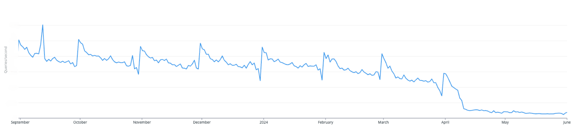
68% decrease in usage tracking update queries, nose-diving from 140 QPS to just 45 QPS!
Master database experienced a significant reduction in CPU utilisation, decreasing by 48.5%—from 35% to just 18%, alleviating considerable strain on its resources.
Replica databases benefited from a 37% decrease in CPU utilisation, dropping from 19% to a more manageable 12%.
Through this optimisation journey, we successfully overcame the challenging database CPU bottlenecks while avoiding the substantial effort and complexity of migrating from SQL to NoSQL. Who would have thought that a calculated leap of faith could save us so much time, effort, and countless sleepless nights? At times, the most effective solutions arise from taking a step back and approaching the problem with a fresh perspective, rather than rushing towards an immediate fix.
Join us
Grab is a leading superapp in Southeast Asia, operating across the deliveries, mobility and digital financial services sectors. Serving over 800 cities in eight Southeast Asian countries, Grab enables millions of people everyday to order food or groceries, send packages, hail a ride or taxi, pay for online purchases or access services such as lending and insurance, all through a single app. Grab was founded in 2012 with the mission to drive Southeast Asia forward by creating economic empowerment for everyone. Grab strives to serve a triple bottom line – we aim to simultaneously deliver financial performance for our shareholders and have a positive social impact, which includes economic empowerment for millions of people in the region, while mitigating our environmental footprint.
Powered by technology and driven by heart, our mission is to drive Southeast Asia forward by creating economic empowerment for everyone. If this mission speaks to you, join our team today!
High availability on a platform like Zabbix is a hard requirement for many users. With native high availability on the Zabbix servers, proxies, and at the frontend through various solutions for web servers, all that’s left is at the database layer. Any downtime in your MariaDB database would disrupt your monitoring availability, at the least on the frontend side of things in case of proxy buffering. Let’s have a look at the easiest way to create a high availability (HA) architecture for Zabbix using MariaDB with built-in Galera clustering – by removing single points of failure from your database and finalizing the HA puzzle for Zabbix.
Architecture overview
Let’s start of with the MariaDB + Galera number one design requirement. For a proper quorum to be made, 3 nodes should be used in the cluster. With only two nodes in a Galera cluster, quorum rules become a bit of a headache, as Galera uses a majority vote (more than half the nodes) to decide if the cluster can still accept writes. In a two-node setup, all is good when the database is online. But when we lose one node, quorum is lost and that node needs to rejoin.
This makes a two-node setup fragile but not impossible, and it does work with Zabbix since we do only have one Zabbix server active at the time. In a split-brain scenario where both nodes either think they are the last to leave, you might have to decide which node you think has your up-to-date data. We will detail both scenario’s, but the principle remains the same. We will use MariaDB as our database and Galera will be used to create a primary/primary cluster. In such a cluster, all nodes in the cluster are writeable, which is great for the Zabbix native HA.
When we look in the Zabbix database, we can see that Zabbix keeps all of it’s Zabbix server HA information and states in the database.
This means that whatever one Zabbix server node writes into the database will also be replicated to all other nodes in the MariaDBGalera cluster.
The design
Knowing what we know now, we can create a very simple design for a solid Zabbix HA setup with Mariadb + Galera. When we have a single Zabbix frontend and we keep to the MariaDB + Galera requirement of having 3 database nodes, we get a fairly simple setup, as seen below.
In this setup, each Zabbix server connects to its own Database node and we don’t need added complexity by using load balancers. However, we do get an automatic failover from the Zabbix servers, as they know exactly which node is active through the database. However, in this situation we are still left with 3 frontends that do not have automatic failover, simply because we do not have database aware Apache or NGINX. This also works in a two database setup, with the side note that you might have quorum issues to manually resolve after an outage:
Adding onto this setup, we could install a VIP, load balancer, or something like HA proxy in front of the frontend to make a failover happen there as well. Keep in mind though, the failover needs to happen based on whether or not the webfrontend can reach a writeable database.
Optional Arbitrator
If you are set on running only 2 database nodes (your wallet is thankful), but still worried about quorums, we can bring in the ARBITRATOR.
If there are only 2 Database nodes in your Galera cluster, not to worry! It’s definitely possible even while maintaining a good quorum resolution in case of outages.
What about load balancing?
Lastly, it is also possible to add load balancing to the mix. Let’s say, for example, you cannot add a VIP to your environment but still need your WEB servers to failover. A load balancer can provide the solution here.
We still prefer to run the Zabbix servers with a direct database connection, but even there a load balancer could be added if you wish. However, please keep in mind that the more load balancers you add, the more complex troubleshooting might become. The whole idea about the setup without load balancers is to have a solid Zabbix setup that is easy to maintain, while providing high availability.
Conclusion
In the end, even with a minimal setup of 2 DB nodes, 2 Zabbix servers, and 2 WEB frontends, we can make a high availability setup. As we’ve shown with Galera, this setup becomes highly flexible, allowing us to run without automatic WEB failover all the way up to including complicated load balancers.
High availability doesn’t have to be overly complicated in a setup like this – it really is all about how far you want to push things. Besides that, in this setup everything is horizontally scalable on the database side. Do keep in mind, however, that Zabbix does still run in an Active/Passive setup.
I hope you enjoyed reading this blog post. If you have any questions or need help configuring anything in your Zabbix setup feel free to contact me and the team at Opensource ICT Solutions. We build a ton of cool stuff like this and more!
Netflix operates at a massive scale, serving hundreds of millions of users with diverse content and features. Behind the scenes, ensuring data consistency, reliability, and efficient operations across various services presents a continuous challenge. At the heart of many critical functions lies the concept of a Write-Ahead Log (WAL) abstraction. At Netflix scale, every challenge gets amplified. Some of the key challenges we encountered include:
Accidental data loss and data corruption in databases
System entropy across different datastores (e.g., writing to Cassandra and Elasticsearch)
Handling updates to multiple partitions (e.g., building secondary indices on top of a NoSQL database)
Data replication (in-region and across regions)
Reliable retry mechanisms forreal time data pipeline at scale
Bulk deletes to database causing OOM on the Key-Value nodes
All the above challenges either resulted in production incidents or outages, consumed significant engineering resources, or led to bespoke solutions and technical debt. During one particular incident, a developer issued an ALTER TABLE command that led to data corruption. Fortunately, the data was fronted by a cache, so the ability to extend cache TTL quickly together with the app writing the mutations to Kafka allowed us to recover. Absent the resilience features on the application, there would have been permanent data loss. As the data platform team, we needed to provide resilience and guarantees to protect not just this application, but all the critical applications we have at Netflix.
Regarding the retry mechanisms for real time data pipelines, Netflix operates at a massive scale where failures (network errors, downstream service outages, etc.) are inevitable. We needed a reliable and scalable way to retry failed messages, without sacrificing throughput.
With these problems in mind, we decided to build a system that would solve all the aforementioned issues and continue to serve the future needs of Netflix in the online data platform space. Our Write-Ahead Log (WAL) is a distributed system that captures data changes, provides strong durability guarantees, and reliably delivers these changes to downstream consumers. This blog post dives into how Netflix is building a generic WAL solution to address common data challenges, enhance developer efficiency, and power high-leverage capabilities like secondary indices, enable cross-region replication for non-replicated storage engines, and support widely used patterns like delayed queues.
API
Our API is intentionally simple, exposing just the essential parameters. WAL has one main API endpoint, WriteToLog, abstracting away the internal implementation and ensuring that users can onboard easily.
/** * WAL request message * namespace: Identifier for a particular WAL * lifecycle: How much delay to set and original write time * payload: Payload of the message * target: Details of where to send the payload */ message WriteToLogRequest { string namespace = 1; Lifecycle lifecycle = 2; bytes payload = 3; Target target = 4; }
A namespace defines where and how data is stored, providing logical separation while abstracting the underlying storage systems. Each namespace can be configured to use different queues: Kafka, SQS, or combinations of multiple. Namespace also serves as a central configuration of settings, such as backoff multiplier or maximum number of retry attempts, and more. This flexibility allows our Data Platform to route different use cases to the most suitable storage system based on performance, durability, and consistency needs.
WAL can assume different personas depending on the namespace configuration.
Persona #1 (Delayed Queues)
In the example configuration below, the Product Data Systems (PDS) namespace uses SQS as the underlying message queue, enabling delayed messages. PDS uses Kafka extensively, and failures (network errors, downstream service outages, etc.) are inevitable. We needed a reliable and scalable way to retry failed messages, without sacrificing throughput. That’s when PDS started leveraging WAL for delayed messages.
Below is the namespace configuration for cross-region replication of EVCache using WAL, which replicates messages from a source region to multiple destinations. It uses Kafka under the hood.
Below is the namespace configuration for supporting mutateItems API in Key-Value, where multiple write requests can go to different partitions and have to be eventually consistent. A key detail in the below configuration is the presence of Kafka and durable_storage. These data stores are required to facilitate two phase commit semantics, which we will discuss in detail below.
An important note is that requests to WAL support at-least once semantics due to the underlying implementation.
Under the Hood
The core architecture consists of several key components working together.
Message Producer and Message Consumer separation: The message producer receives incoming messages from client applications and adds them into the queue, while the message consumer processes messages from the queue and sends them to the targets. Because of this separation, other systems can bring their own pluggable producers or consumers, depending on their use cases. WAL’s control plane allows for a pluggable model, which, depending on the use-case, allows us to switch between different message queues.
SQS and Kafka with a dead letter queue by default: Every WAL namespace has its own message queue and gets a dead letter queue (DLQ) by default, because there can be transient errors and hard errors. Application teams using Key-Value abstraction simply need to toggle a flag to enable WAL and get all this functionality without needing to understand the underlying complexity.
Kafka-backed namespaces: handle standard message processing
SQS-backed namespaces: support delayed queue semantics (we added custom logic to go beyond the standard defaults enforced in terms of delay, size limits, etc)
Complex multi-partition scenarios: use queues and durable storage
Target Flexibility: The messages added to WAL are pushed to the target datastores. Targets can be Cassandra databases, Memcached caches, Kafka queues, or upstream applications. Users can specify the target via namespace configuration and in the API itself.
Architecture of WAL
Deployment Model
WAL is deployed using the Data Gateway infrastructure. This means that WAL deployments automatically come with mTLS, connection management, authentication, runtime and deployment configurations out of the box.
Each data gateway abstraction (including WAL) is deployed as a shard. A shard is a physical concept describing a group of hardware instances. Each use case of WAL is usually deployed as a separate shard. For example, the Ads Events service will send requests to WAL shard A, while the Gaming Catalog service will send requests to WAL shard B, allowing for separation of concerns and avoiding noisy neighbour problems.
Each shard of WAL can have multiple namespaces. A namespace is a logical concept describing a configuration. Each request to WAL has to specify its namespace so that WAL can apply the correct configuration to the request. Each namespace has its own configuration of queues to ensure isolation per use case. If the underlying queue of a WAL namespace becomes the bottleneck of throughput, the operators can choose to add more queues on the fly by modifying the namespace configurations. The concept of shards and namespaces is shared across all Data Gateway Abstractions, including Key-Value, Counter, Timeseries, etc. The namespace configurations are stored in a globally replicated Relational SQL database to ensure availability and consistency.
Deployment model of WAL
Based on certain CPU and network thresholds, the Producer group and the Consumer group of each shard will (separately) automatically scale up the number of instances to ensure the service has low latency, high throughput and high availability. WAL, along with other abstractions, also uses the Netflix adaptive load shedding libraries and Envoy to automatically shed requests beyond a certain limit. WAL can be deployed to multiple regions, so each region will deploy its own group of instances.
Solving different flavors of problems with no change to the core architecture
The WAL addresses multiple data reliability challenges with no changes to the core architecture:
Data Loss Prevention: In case of database downtime, WAL can continue to hold the incoming mutations. When the database becomes available again, replay mutations back to the database. The tradeoff is eventual consistency rather than immediate consistency, and no data loss.
Generic Data Replication: For systems like EVCache (using Memcached) and RocksDB that do not support replication by default, WAL provides systematic replication (both in-region and across-region). The target can be another application, another WAL, or another queue — it’s completely pluggable through configuration.
System Entropy and Multi-Partition Solutions: Whether dealing with writes across two databases (like Cassandra and Elasticsearch) or mutations across multiple partitions in one database, the solution is the same — write to WAL first, then let the WAL consumer handle the mutations. No more asynchronous repairs needed; WAL handles retries and backoff automatically.
Data Corruption Recovery: In case of DB corruptions, restore to the last known good backup, then replay mutations from WAL omitting the offending write/mutation.
There are some major differences between using WAL and directly using Kafka/SQS. WAL is an abstraction on the underlying queues, so the underlying technology can be swapped out depending on use cases with no code changes. WAL emphasizes an easy yet effective API that saves users from complicated setups and configurations. We leverage the control plane to pivot technologies behind WAL when needed without app or client intervention.
WAL usage at Netflix
Delay Queue
The most common use case for WAL is as a Delay Queue. If an application is interested in sending a request at a certain time in the future, it can offload its requests to WAL, which guarantees that their requests will land after the specified delay.
Netflix’s Live Origin processes and delivers Netflix live stream video chunks, storing its video data in a Key-Value abstraction backed by Cassandra and EVCache. When Live Origin decides to delete certain video data after an event is completed, it issues delete requests to the Key-Value abstraction. However, the large amount of delete requests in a short burst interfere with the more important real-time read/write requests, causing performance issues in Cassandra and timeouts for the incoming live traffic. To get around this, Key-Value issues the delete requests to WAL first, with a random delay and jitter set for each delete request. WAL, after the delay, sends the delete requests back to Key-Value. Since the deletes are now a flatter curve of requests over time, Key-Value is then able to send the requests to the datastore with no issues.
Requests being spread out over time through delayed requests
Additionally, WAL is used by many services that utilize Kafka to stream events, including Ads, Gaming, Product Data Systems, etc. Whenever Kafka requests fail for any reason, the client apps will send WAL a request to retry the kafka request with a delay. This abstracts away the backoff and retry layer of Kafka for many teams, increasing developer efficiency.
Backoff and delayed retries for clients producing to KafkaBackoff and delayed retries for clients consuming from Kafka
Cross-Region Replication
WAL is also used for global cross-region replication. The architecture of WAL is generic and allows any datastore/applications to onboard for cross-region replication. Currently, the largest use case is EVCache, and we are working to onboard other storage engines.
EVCache is deployed by clusters of Memcached instances across multiple regions, where each cluster in each region shares the same data. Each region’s client apps will write, read, or delete data from the EVCache cluster of the same region. To ensure global consistency, the EVCache client of one region will replicate write and delete requests to all other regions. To implement this, the EVCache client that originated the request will send the request to a WAL corresponding to the EVCache cluster and region.
Since the EVCache client acts as the message producer group in this case, WAL only needs to deploy the message consumer groups. From there, the multiple message consumers are set up to each target region. They will read from the Kafka topic, and send the replicated write or delete requests to a Writer group in their target region. The Writer group will then go ahead and replicate the request to the EVCache server in the same region.
EVCache Global Cross-Region Replication Implemented through WAL
The biggest benefits of this approach, compared to our legacy architecture, is being able to migrate from multi-tenant architecture to single tenant architecture for the most latency sensitive applications. For example, Live Origin will have its own dedicated Message Consumer and Writer groups, while a less latency sensitive service can be multi-tenant. This helps us reduce the blast radius of the issues and also prevents noisy neighbor issues.
Multi-Table Mutations
WAL is used by Key-Value service to build the MutateItems API. WAL enables the API’s multi-table and multi-id mutations by implementing 2-phase commit semantics under the hood. For this discussion, we can assume that Key-Value service is backed by Cassandra, and each of its namespaces represents a certain table in a Cassandra DB.
When a Key-Value client issues a MutateItems request to Key-Value server, the request can contain multiple PutItems or DeleteItems requests. Each of those requests can go to different ids and namespaces, or Cassandra tables.
The MutateItems request operates on an eventually consistent model. When the Key-Value server returns a success response, it guarantees that every operation within the MutateItemsRequest will eventually complete successfully. Individual put or delete operations may be partitioned into smaller chunks based on request size, meaning a single operation could spawn multiple chunk requests that must be processed in a specific sequence.
Two approaches exist to ensure Key-Value client requests achieve success. The synchronous approach involves client-side retries until all mutations complete. However, this method introduces significant challenges; datastores might not natively support transactions and provide no guarantees about the entire request succeeding. Additionally, when more than one replica set is involved in a request, latency occurs in unexpected ways, and the entire request chain must be retried. Also, partial failures in synchronous processing can leave the database in an inconsistent state if some mutations succeed while others fail, requiring complex rollback mechanisms or leaving data integrity compromised. The asynchronous approach was ultimately adopted to address these performance and consistency concerns.
Given Key-Value’s stateless architecture, the service cannot maintain the mutation success state or guarantee order internally. Instead, it leverages a Write-Ahead Log (WAL) to guarantee mutation completion. For each MutateItems request, Key-Value forwards individual put or delete operations to WAL as they arrive, with each operation tagged with a sequence number to preserve ordering. After transmitting all mutations, Key-Value sends a completion marker indicating the full request has been submitted.
The WAL producer receives these messages and persists the content, state, and ordering information to a durable storage. The message producer then forwards only the completion marker to the message queue. The message consumer retrieves these markers from the queue and reconstructs the complete mutation set by reading the stored state and content data, ordering operations according to their designated sequence. Failed mutations trigger re-queuing of the completion marker for subsequent retry attempts.
Architecture of Multi-Table Mutations through WALSequence diagram for Multi-Table Mutations through WAL
Closing Thoughts
Building Netflix’s generic Write-Ahead Log system has taught us several key lessons that guided our design decisions:
Pluggable Architecture is Core: The ability to support different targets, whether databases, caches, queues, or upstream applications, through configuration rather than code changes has been fundamental to WAL’s success across diverse use cases.
Leverage Existing Building Blocks: We had control plane infrastructure, Key-Value abstractions, and other components already in place. Building on top of these existing abstractions allowed us to focus on the unique challenges WAL needed to solve.
Separation of Concerns Enables Scale: By separating message processing from consumption and allowing independent scaling of each component, we can handle traffic surges and failures more gracefully.
Systems Fail — Consider Tradeoffs Carefully: WAL itself has failure modes, including traffic surges, slow consumers, and non-transient errors. We use abstractions and operational strategies like data partitioning and backpressure signals to handle these, but the tradeoffs must be understood.
Future work
We are planning to add secondary indices in Key-Value service leveraging WAL.
WAL can also be used by a service to guarantee sending requests to multiple datastores. For example, a database and a backup, or a database and a queue at the same time etc.
Acknowledgements
Launching WAL was a collaborative effort involving multiple teams at Netflix, and we are grateful to everyone who contributed to making this idea a reality. We would like to thank the following teams for their roles in this launch.
Caching team — Additional thanks to Shih-Hao Yeh, Akashdeep Goel for contributing to cross region replication for KV, EVCache etc. and owning this service.
Product Data System team — Carlos Matias Herrero, Brandon Bremen for contributing to the delay queue design and being early adopters of WAL giving valuable feedback.
KeyValue and Composite abstractions team — Raj Ummadisetty for feedback on API design and mutateItems design discussions. Rajiv Shringifor feedback on API design.
Kafka and Real Time Data Infrastructure teams — Nick Mahilani for feedback and inputs on integrating the WAL client into Kafka client. Sundaram Ananthanarayan for design discussions around the possibility of leveraging Flink for some of the WAL use cases.
Joseph Lynch for providing strategic direction and organizational support for this project.
We’re not burying the lede on this one: you can now connect Cloudflare Workers to your PlanetScale databases directly and ship full-stack applications backed by Postgres or MySQL.
We’ve teamed up with PlanetScale because we wanted to partner with a database provider that we could confidently recommend to our users: one that shares our obsession with performance, reliability and developer experience. These are all critical factors for any development team building a serious application.
Now, when connecting to PlanetScale databases, your connections are automatically configured for optimal performance with Hyperdrive, ensuring that you have the fastest access from your Workers to your databases, regardless of where your Workers are running.
Building full-stack
As Workers has matured into a full-stack platform, we’ve introduced more options to facilitate your connectivity to data. With Workers KV, we made it easy to store configuration and cache unstructured data on the edge. With D1 and Durable Objects, we made it possible to build multi-tenant apps with simple, isolated SQL databases. And with Hyperdrive, we made connecting to external databases fast and scalable from Workers.
Today, we’re introducing a new choice for building on Cloudflare: Postgres and MySQL PlanetScale databases, directly accessible from within the Cloudflare dashboard. Link your Cloudflare and PlanetScale accounts, stop manually copying API keys back-and-forth, and connect Workers to any of your PlanetScale databases (production or otherwise!).
Connect to a PlanetScale database — no figuring things out on your own
Postgres and MySQL are the most popular options for building applications, and with good reason. Many large companies have built and scaled on these databases, providing for a robust ecosystem (like Cloudflare!). And you may want to have access to the power, familiarity, and functionality that these databases provide.
Importantly, all of this builds on Hyperdrive, our distributed connection pooler and query caching infrastructure. Hyperdrive keeps connections to your databases warm to avoid incurring latency penalties for every new request, reduces the CPU load on your database by managing a connection pool, and can cache the results of your most frequent queries, removing load from your database altogether. Given that about 80% of queries for a typical transactional database are read-only, this can be substantial — we’ve observed this in reality!
No more copying credentials around
Starting today, you can connect to your PlanetScale databases from the Cloudflare dashboard in just a few clicks. Connecting is now secure by default with a one-click password rotation option, without needing to copy and manage credentials back and forth. A Hyperdrive configuration will be created for your PlanetScale database, providing you with the optimal setup to start building on Workers.
And the experience spans both Cloudflare and PlanetScale dashboards: you can also create and view attached Hyperdrive configurations for your databases from the PlanetScale dashboard.
By automatically integrating with Hyperdrive, your PlanetScale databases are optimally configured for access from Workers. When you connect your database via Hyperdrive, Hyperdrive’s Placement system automatically determines the location of the database and places its pool of database connections in Cloudflare data centers with the lowest possible latency.
When one of your Workers connects to your Hyperdrive configuration for your PlanetScale database, Hyperdrive will ensure the fastest access to your database by eliminating the unnecessary roundtrips included in a typical database connection setup. Hyperdrive will resolve connection setup within the Hyperdrive client and use existing connections from the pool to quickly serve your queries. Better yet, Hyperdrive allows you to cache your query results in case you need to scale for high-read workloads.
This is a peek under the hood of how Hyperdrive makes access to PlanetScale as fast as possible. We’ve previously blogged about Hyperdrive’s technical underpinnings — it’s worth a read. And with this integration with Hyperdrive, you can easily connect to your databases across different Workers applications or environments, without having to reconfigure your credentials. All in all, a perfect match.
Get started with PlanetScale and Workers
With this partnership, we’re making it trivially easy to build on Workers with PlanetScale. Want to build a new application on Workers that connects to your existing PlanetScale cluster? With just a few clicks, you can create a globally deployed app that can query your database, cache your hottest queries, and keep your database connections warmed for fast access from Workers.
Connect directly to your PlanetScale MySQL or Postgres databases from the Cloudflare dashboard, for optimal configuration with Hyperdrive.
Grab operates as a dynamic ecosystem involving partners and various service providers, necessitating real-time intelligence and decision-making for seamless integration and service delivery. To facilitate this, GrabDeveloper serves as Grab’s centralized platform for developers and partners. It supports API integration, partner onboarding, and product management. It also provides tech support through staging and production portals with detailed documentation.
Working alongside Developer Home, Partner Gateway acts as Grab’s secure interface for exposing APIs to third-party entities. It enables seamless interactions between Grab’s hosted services and external consumers, such as mobile apps, web browsers, and partners. Partner Gateway enhances the experience by offering advanced metrics tracking through time-series charts and dashboards. Partner Gateway delivers actionable insights that ensure high performance, reliability, and user satisfaction in application integrations with Grab services.
Use cases
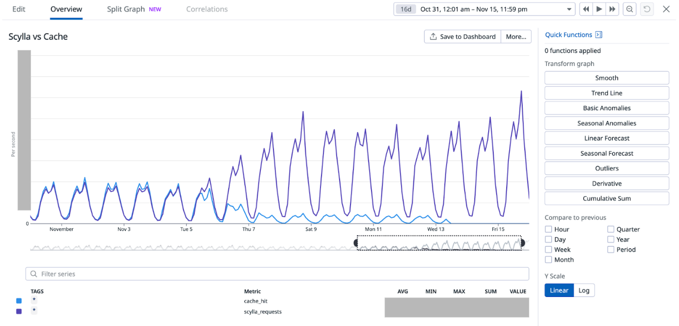
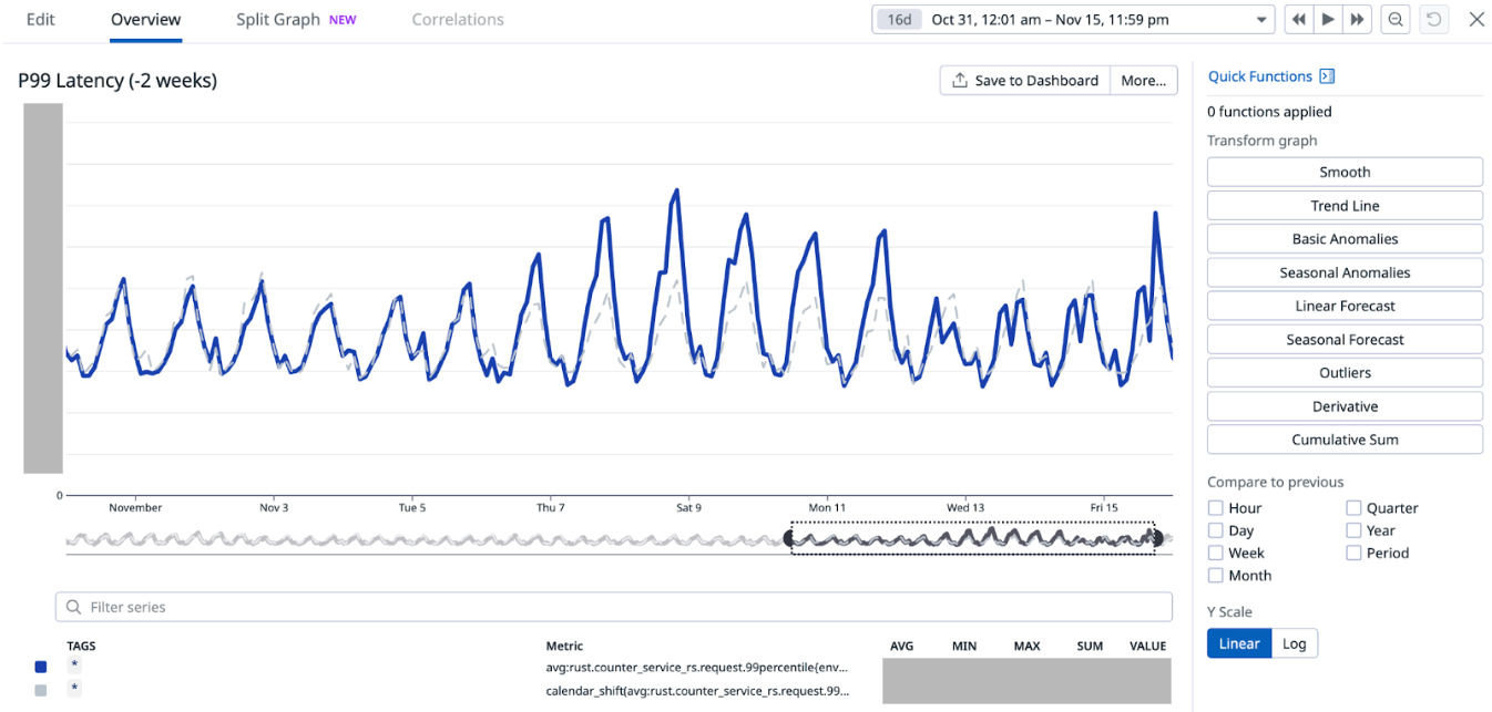
Let’s explore GrabDeveloper integration use cases with one of our partners, whom we’ll refer to as “Alpha.” Alpha is a company that specializes in producing and distributing a diverse range of perishable goods. To optimize their operations, time-series charts tracking API traffic request status codes and average API response times play a crucial role.
API traffic request service status codes chart
Time-series charts tracking API traffic request status codes offer valuable insights into the performance and reliability of APIs used for managing supply chain logistics, customer orders, and distribution networks. By monitoring these status codes, Alpha can promptly detect and resolve disruptions or failures in their digital systems, ensuring seamless operations and minimizing downtime.
Figure 1: API traffic chart from 5th Jan 2025 to 4th Mar 2025.
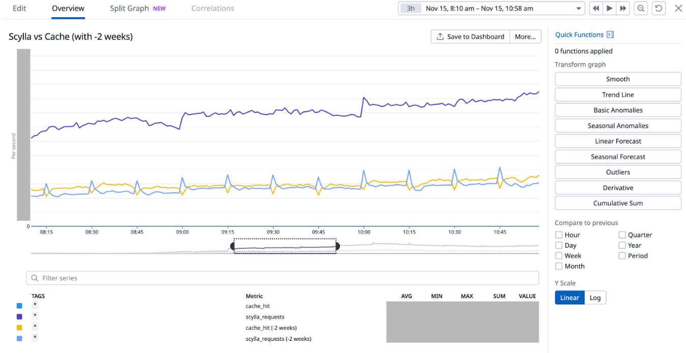
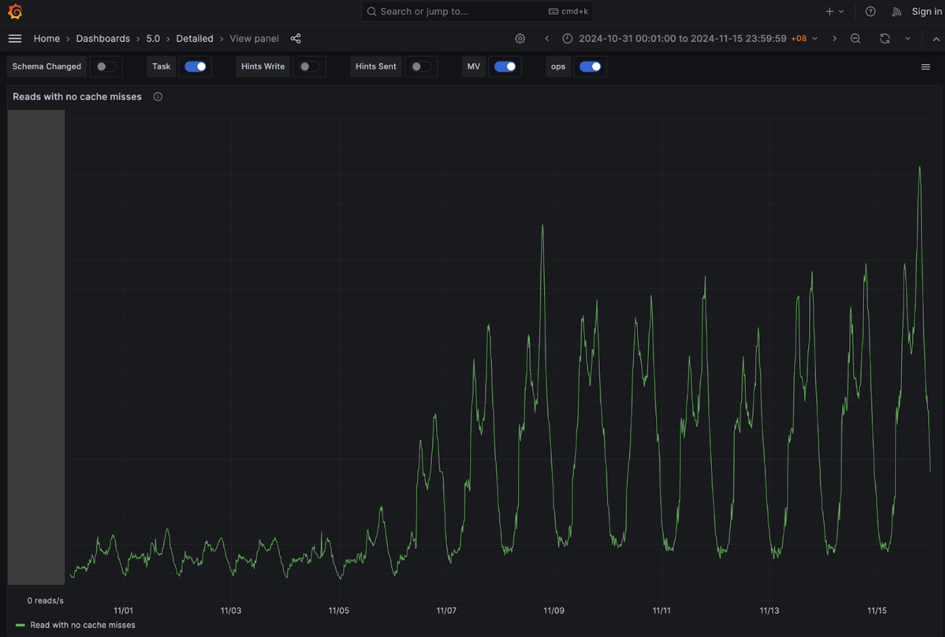
API average response times chart
Analyzing average response times helps the company maintain efficient communication between various systems, enhancing the speed and reliability of transactions and data exchanges. This proactive monitoring supports Alpha in delivering consistent, high-quality service to customers and partners, ultimately contributing to improved operational efficiency and customer satisfaction.
Analyzing average response times enables a company to ensure efficient communication across various systems, enhancing transaction speed and data exchange reliability. Proactive monitoring helps Alpha deliver consistent, high-quality service to customers and partners, boosting operational efficiency and customer satisfaction.
Figure 2: Average response time chart from 12 Mar 2025 3am to 12 Mar 2025 3pm (Endpoints are mocked for security purposes).
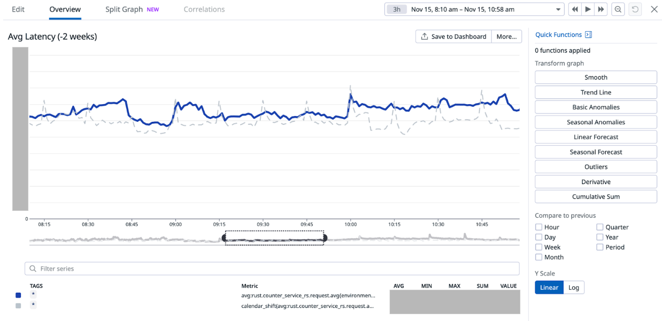
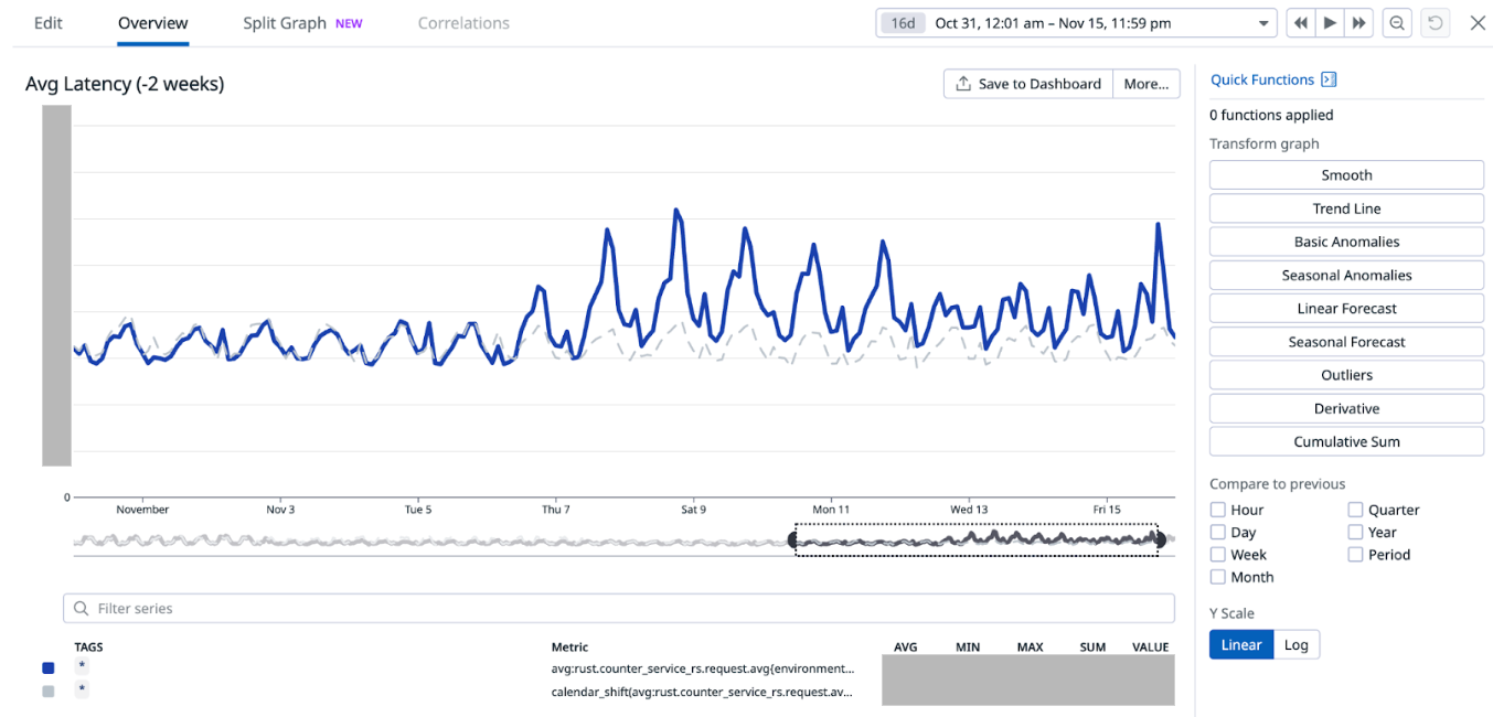
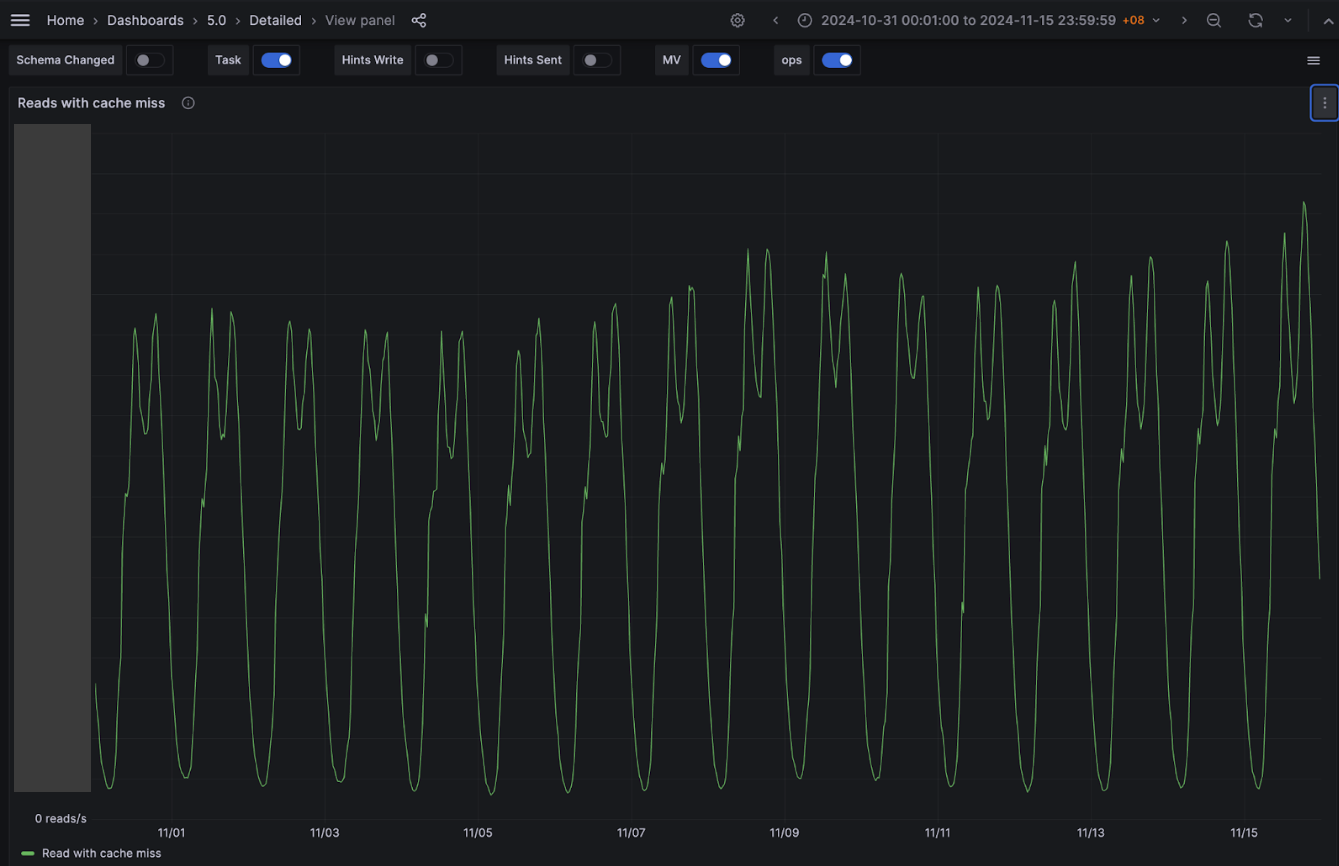
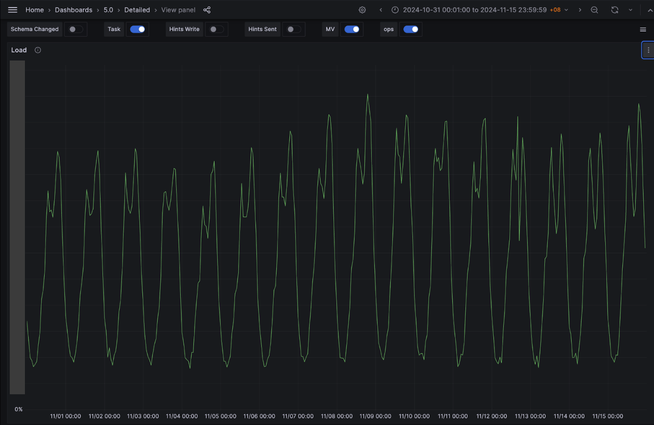
Endpoint status dashboard
For Alpha, the endpoint status dashboard delivers real-time insights into API performance, enabling swift issue resolution and seamless integration with the company’s systems. The dashboard enhances service reliability, supports business operations, and ensures uninterrupted data exchange, all of which are critical for Alpha’s business processes and customer satisfaction. Furthermore, the transparency and reliability provided by the dashboard strengthens trust in the partnership, ensuring Alpha to confidently rely on the integration to drive their digital initiatives and operational goals.
Figure 3: Endpoint status dashboard of express API for company Alpha. *Endpoints are mocked for security purposes.
Why choose Apache Pinot and what is it?
To accommodate these use cases, we need a backend storage system engineered for low-latency queries across a wide range of temporal intervals, spanning from one-hour snapshots to 30-day retrospective analyses, whereby it could contain up to ~6.8 billion rows of data in a 30 day period for a particular dataset. This led us to choose Apache Pinot for these use cases, a distributed Online Analytical Processing (OLAP) system designed for low-latency analytical queries on large-scale data with millisecond query latencies.
Apache Pinot is a real-time distributed OLAP datastore designed to deliver low-latency analytics on large-scale data. It is optimized for high-throughput ingestion and real-time query processing making it ideal for scenarios such as user-facing analytics, dashboards, and anomaly detection. Apache Pinot supports complex queries, including aggregations and filtering. It delivers sub-second response times by leveraging techniques like columnar storage, indexing, and data partitioning to achieve efficient query execution.
Data ingestion process
Figure 4: Data ingestion process.
API call initiation: An API call is made on the partner application and routed through the Partner Gateway.
Metric tracking: Dimensions such as client ID, partner ID, status code, endpoint, metric name, timestamp, and value (which is the metric) are tracked and uploaded to Datadog, a cloud-based monitoring platform.
Kafka message transformation: Within the partner gateway code, an Apache Kafka Producer converts these metrics into Kafka messages and stores them in a Kafka Topic. Grab utilizes Protobuf for serialization and deserialization of Kafka messages. Since Grab’s Golang Kafka ecosystem does not use the Confluent Schema Registry, Kafka messages must be serialized with a magic byte which indicates that they are using Confluent’s Schema Registry, followed by the Schema ID.
Serialization via Apache Flink: Serialization is managed using Apache Flink, an open-source stream processing framework. This ensures compatibility with the Confluent Schema Registry Protobuf Decoder plugin on Apache Pinot. The messages are then written to a separate Kafka Topic.
Ingestion to Apache Pinot: Messages from the Kafka Topic containing the magic byte are ingested directly into Pinot, which references the Confluent Schema Registry to accurately deserialize the messages.
Query execution: Queries on the Pinot table can be executed via the Pinot Rest Proxy API.
Data visualization: Users can view their project charts and dashboards on the GrabDeveloper Home UI, where data points are retrieved from queries executed in step 6.
Challenges faced
During the initial setup, we encountered significant performance challenges when executing aggregation queries on large datasets exceeding 150GB. Specifically, attempts to retrieve and process data for periods ranging from 20 to 30 days resulted in frequent timeout issues as the queries took longer than 10 seconds. This was particularly concerning as it compromised our ability to meet our Service Level Agreement (SLA) of delivering query results within 300 milliseconds. The existing query infrastructure struggled to efficiently manage the volume and complexity of data within the required timeframe, necessitating optimization efforts to improve performance and reliability.
Solution
Drawing from the insights gained on the limitations of our initial solutions, we implemented these strategic optimizations to significantly enhance our table’s performance.
Partitioning by metric name
Improved data locality: Partitioning the Kafka Topic by metric name ensures that related data is grouped together. When a query filters on a specific metric, Pinot can directly access the relevant partitions, minimizing the need to scan unrelated data. This significantly reduces I/O overhead and processing time.
Efficient query pruning: By physically partitioning data, only the servers holding the relevant partitions are queried. This leads to more efficient query pruning, as irrelevant data is excluded early in the process, further optimizing performance.
Enhanced parallel processing: Partitioning enables Pinot to distribute queries across multiple nodes, allowing different metrics to be processed in parallel. This leverages distributed computing resources, accelerating query execution and improving scalability for large datasets.
Column based on aggregation intervals
Table 1
Facilitates time-based aggregations: Rounded time columns (e.g., Timestamp_1h for hourly intervals) group data into coarser time buckets, enabling efficient aggregations such as hourly or daily metrics. This simplifies indexing and optimizes storage by precomputing aggregates for specific time intervals.
Efficient data filtering: Rounded time columns allow for precise filtering of data within specific aggregation intervals. For example, the query SELECT SUM(Value) FROM Table WHERE Timestamp_1h = '2025-01-20 01:00:00' can exclude irrelevant columns (e.g., column 2) and focus only on rows within the specified time interval, further enhancing query efficiency.
Utilizing the Star-tree index in Apache Pinot
The Star-tree Index in Apache Pinot is an advanced indexing structure that enhances query performance by pre-aggregating data across multiple dimensions (e.g., D1, D2). It features a hierarchical tree with a root node, leaf nodes (holding up to T records), and non-leaf nodes that split into child nodes when exceeding T records. Special star nodes store pre-aggregated records by omitting the splitting dimension. The tree is constructed based on a dimensionSplitOrder, dictating node splitting at each level.
dimensionsSplitOrder: This specifies the order in which dimensions are split at each level of the tree. The order is “Metric”, “Endpoint”, “Timestamp_1h”. This means the tree will first split by Metric, then by Endpoint, and finally by Timestamp_1h.
skipStarNodeCreationForDimensions: This array is empty, indicating that star nodes will be created for all dimensions specified in the split order. No dimensions are omitted from star node creation.
functionColumnPairs: This specifies the aggregation functions to be applied to columns when creating star nodes. The configuration includes “AVG__Value”, meaning the average of the “Value” column will be calculated and stored in star nodes.
maxLeafRecords: This is set to 1, indicating that each leaf node will contain only one record. If a node exceeds this number, it will split into child nodes.
Star-tree diagram
Figure 5: Star-tree Index Structure.
Components:
Root node (orange): This is the starting point for traversing the tree structure.
Leaf node (blue): These nodes contain up to a configurable number of records, denoted by T. In this configuration, maxLeafRecords is set to 1, meaning each leaf node will contain a maximum of one record.
Non-leaf node (green): These nodes will split into child nodes if they exceed the maxLeafRecords threshold. Since maxLeafRecords is set to 1, any node with more than one record will split.
Star-node (yellow): These nodes store pre-aggregated records by omitting the dimension used for splitting at that level. This helps in reducing the data size and improving query performance.
Example:
A practical explanation of the start-tree diagram would be to display the star-tree documents in a table format along with the sample queries used to retrieve the data.
Figure 6: Chart of query latency with and without optimization.
The graph above in Figure 6, provides a comparison analysis of query performance, showcasing the significant improvements achieved through the implemented optimization solutions. The query execution times are significantly reduced, as evidenced by the logarithmic scale values.
For the first query which calculates the latency for a particular aggregation interval, the log scale indicates a reduction from 4.64 to 2.32, translating to a decrease in query latency from 43,713 to 209 milliseconds.
Similarly, the second query, which aggregates the sum of the latency based on the tags for a particular metric, shows a log scale reduction from 3.71 to 1.54, with query latency improving from 5,072 to 35 milliseconds. These results underscore the efficacy of optimization in enhancing query performance, enabling faster data retrieval and processing
Tradeoffs
Star-tree indexes in Apache Pinot are designed to significantly enhance query performance by pre-computing aggregations. This approach allows for rapid query execution by utilizing pre-calculated results, rather than computing aggregations on-the-fly. However, this performance boost comes with a tradeoff in terms of storage space.
Before implementing the Star-tree index, the total storage size for 30 days of data was approximately 192GB. With the Star-tree index, this increased to 373GB, nearly doubling the storage requirements. Despite the increase in storage, the performance benefits substantially outweigh the costs associated with additional storage.
The cost impact is relatively minor. We utilize AWS gp3 EBS volumes, which roughly cost $14.48 USD monthly for the extra table (calculated as 0.08 USD x 181 GB). This cost is considered insignificant when compared to the substantial gains in query performance. Alternatively, precomputing the metrics via an ETL job is also feasible; however, it is less cost-effective due to the additional expenses required to maintain the pipeline.
The decision to use Star-tree indexes is justified by the dramatic improvement in query speed, which enhances user experience and efficiency. The modest increase in storage costs is a worthwhile investment for achieving optimal performance.
Conclusion
In conclusion, Grab’s integration of Apache Pinot as a backend solution within the Partner Gateway represents a forward-thinking strategy to meet the evolving demands of real-time analytics. Apache Pinot’s ability to deliver low-latency queries empowers our partners with immediate, actionable insights into API performance that enhances their integration experience and operational efficiency. This is crucial for partners who require rapid data access to make informed decisions and optimize their services.
The adoption of Star-tree indexing within Pinot further refines our analytics infrastructure by strategically balancing the trade-offs between query latency and storage costs. This optimization ensures Partner Gateway can support a diverse range of use cases with subsecond query latencies while maintaining high performance and reliability in service delivery reinforcing Grab’s commitment to delivering superior performance across its ecosystem.
Ultimately, the integration of Apache Pinot enhances Grab’s real-time analytics capabilities while empowering the company to drive innovation and consistently deliver exceptional service to both partners and users.
Credits to Manh Nguyen from the Coban Infrastructure Team, Michael Wengle from the Midas Team and Yuqi Wang from the DevHome team.
Join us
Grab is a leading superapp in Southeast Asia, operating across the deliveries, mobility and digital financial services sectors. Serving over 800 cities in eight Southeast Asian countries, Grab enables millions of people everyday to order food or groceries, send packages, hail a ride or taxi, pay for online purchases or access services such as lending and insurance, all through a single app. Grab was founded in 2012 with the mission to drive Southeast Asia forward by creating economic empowerment for everyone. Grab strives to serve a triple bottom line – we aim to simultaneously deliver financial performance for our shareholders and have a positive social impact, which includes economic empowerment for millions of people in the region, while mitigating our environmental footprint.
Powered by technology and driven by heart, our mission is to drive Southeast Asia forward by creating economic empowerment for everyone. If this mission speaks to you, join our team today!
At Grab, our journey towards a more robust and scalable data ecosystem has been a continuous evolution.
Considering the size of our data lake and complexity of our ecosystem, with businesses spanning across ride hailing, food delivery, and financial services, we have been long past the point where a single centrally managed data warehouse could serve all these data needs. Over its first decade, Grab experienced dramatic growth. Like most growing businesses, teams in Grab prioritised delivering new features to meet the demands of their users. This meant that the task of data maintenance had to take a back seat so that development and stabilisation works can be focused to keep up with the growth. However, to prepare Grab for the next 10 years, especially for a future where AI is likely to play an important role, our leadership understood the need for high quality data foundation and gave a mandate to our data teams to uplevel our entire enterprise data ecosystem.
Acknowledging the rising need for data-driven insights and the continuous expansion of our data repository, we initiated our data mesh journey, named the Signals Marketplace, in 2024.
However, this journey was far from simple. We encountered several critical challenges that required a significant transformation in our approach to data management. Some of the challenges encountered include:
High volume and variety of data being generated: Grab’s diverse operations created both opportunities and complexities. Effectively harnessing this wealth of information required a scalable, streamlined and accessible approach.
Gaps in data ownership: As our data landscape expanded, maintaining data quality and reliability became increasingly difficult without clear lines of ownership and accountability. This often led to ad-hoc discussions and delays in resolving data related issues. Since it was difficult to trust the reliability of an existing pipeline, teams were likely to create duplicate pipelines just so they have something they can control.
Unscalable reliance on central Data Engineering (DE) team: Our traditional reliance on a central DE team to curate and serve all data needs was becoming a bottleneck. This centralised model struggled to keep pace with the distributed nature of data creation and consumption across various product and engineering teams.
Lack of communication between data consumers and producers: Data producers are unaware of downstream dependencies of their data which led to several instances of critical pipelines breaking because of upstream changes.
No single source of truth: While we did have a central data warehouse, it still left a lot of data gaps across Grab’s many business lines. Teams would struggle to identify the correct data definitions and reliable sources of truth.
Varied sophistication of data practitioners: Different teams have different levels of expertise in regards to data. Some teams had dedicated data engineers, but many didn’t.
To address these challenges, we made a strategic decision to adopt a data mesh architecture. Data mesh is a decentralised approach to data management that treats data as a product, owned and served by domain specific teams. This paradigm shift empowers teams closest to the data to take responsibility for its quality, reliability, and accessibility.
Our primary goal in adopting a data mesh was to significantly increase the reusability and reliability of our data assets across the organisation. By fostering a culture of data ownership and providing the necessary tools and processes, we aimed to unlock the full potential of our data to drive innovation and better serve our users and partners.
Certification
A cornerstone of our data mesh implementation is the concept of data certification. We believe that clearly identifying high quality, trustworthy datasets is crucial for both data producers and consumers.
Why certification?
Certification offers significant benefits to both sides of the data ecosystem. Data producers can clearly define and communicate the expectations and guarantees associated with their certified data assets, like defining Service Level Agreements (SLAs) for engineering services. This includes aspects like schema, data quality, and freshness. For data consumers, certification provides the confidence to readily discover and utilise these assets. Knowing that they come with stronger reliability guarantees and clear documentation, data consumers can confidently “shop” for certified data products, reducing the need for extensive validation and ad-hoc inquiries.
Figure 1: Concept of data certification
To achieve widespread data certification, we focused on several key enablers:
Ownership: Establishing decentralised ownership and accountability is fundamental and non-trivial. We clearly identified teams which we call Data Domains, individuals responsible as Business Data Owners (BDOs), and Technical Data Owners (TDOs) for the upkeep, usability, documentation, and associated Scheduled Large Orders (SLOs) of each data product. This step was bootstrapped by leveraging the identification of the data asset creator’s team. However, if the creator had changed teams or left the company, the initial mapping of Domain <> Data Asset needs to be reviewed by the Domain Leads.
Data contract: We introduced data contracts as formal agreements between data producers and consumers. These contracts define the schema, SLA guarantees (including freshness, completeness, and retention policies), notice period for changes, and communication channels for a data product. Data certification helps set clear expectations and ensures reliability across data pipelines.
Data operational excellence
To further enhance accountability and ensure adherence to data contracts, we implemented automated Data Production Incidents (DPIs) for breached contracts. When data quality tests are done on data availability, timeliness, consistency, completeness, accuracy, validity, or other reliability guarantees fail, a DPI ticket is automatically created and assigned to the TDO. This system aims to standardise and drive accountability in investigating and fixing issues related to reliability guarantees within Data Contracts. The goal is for teams to acknowledge and fix the root cause of the DPIs.
Operationalisation and outcomes
To drive the adoption of data certification and the principles of data mesh across Grab, we focused on the following north star metric: percentage of queries hitting certified assets (%). This metric serves as a direct indicator of the reusability and trust in our certified data products. It also helps teams prioritise their certification efforts towards the most frequently used tables. It essentially pushes every data team in two synergistic directions:
To certify their most used datasets.
To query only certified datasets as much as possible.
Operationalisation
The successful operationalisation of our data mesh and certification efforts relied on several key factors listed below:
Executive buy-in: Strong leadership support was crucial in driving this organisational change and emphasising the importance of data as a product.
Organisation-wide push with clear measurable reporting: We implemented an organisation-wide initiative with clearly defined goals and measurable targets for data certification. Progress is tracked and reported to ensure accountability and drive momentum.
Dashboard to guide Grabbers target most used tables: Dashboards and tooling likely within Hubble, provided visibility into data usage patterns, guiding teams to prioritise the certification of their most popular and impactful datasets.
Outcomes
As a result of these efforts, we have observed significant positive outcomes:
75% of Grab queries hitting certified assets: We achieved a significant milestone with 75% of Grab’s data queries now targeting certified assets. This indicates a strong adoption of certified data products and a growing trust in their reliability.
Active deprecation of assets: The focus on data ownership and the push for certification has also led to increased visibility into our data landscape, allowing us to identify and actively deprecate redundant and duplicated data assets. Deprecated tables increases 400% year over year (YoY). This not only improves efficiency but also reduces the complexity and cost of maintaining our data infrastructure.
Accelerated innovation and cross-domain reusability: Prior to data mesh, every team often resorted to building their own data sources which leads to lower quality outcomes and slower turn around time. Today, internet of things datasets (IoT) like weather data collected by one team can now be reused by another team to optimise marketplace decisions — a practical step toward a more connected data ecosystem.
Beyond these individual instances, we observe a convergence across Grab towards most used datasets, with the number of P80 datasets (the top 80% of Grab’s most used data) reducing by over 58% since the start of the campaign.
What’s next
While we have made significant strides in our data mesh journey, we recognise that this is an ongoing evolution. This progress wouldn’t be as smooth sailing without the platforms we build for data management and observability. In our next article, we will be delving into the enhancements for crucial tooling and platforms like Genchi (in-house data quality observational tool) and Hubble (metadata management platform, built on DataHub and Grab proprietary technology), which underpin our data mesh vision and enable greater data reliability and reusability.
Massive credits to Grab’s leadership, Mohan Krishnan and Nikhil Dwarakanath, as well as Data owners on driving this Grab-wide effort to build strong data foundations in Grab. Grab’s data mesh would not have been possible without the commitment of all data owners to certify and curate their data products.
Join us
Grab is a leading superapp in Southeast Asia, operating across the deliveries, mobility and digital financial services sectors. Serving over 800 cities in eight Southeast Asian countries, Grab enables millions of people everyday to order food or groceries, send packages, hail a ride or taxi, pay for online purchases or access services such as lending and insurance, all through a single app. Grab was founded in 2012 with the mission to drive Southeast Asia forward by creating economic empowerment for everyone. Grab strives to serve a triple bottom line – we aim to simultaneously deliver financial performance for our shareholders and have a positive social impact, which includes economic empowerment for millions of people in the region, while mitigating our environmental footprint.
Powered by technology and driven by heart, our mission is to drive Southeast Asia forward by creating economic empowerment for everyone. If this mission speaks to you, join our team today!
Ten years ago, we announced the general availability of Amazon Aurora, a database that combined the speed and availability of high-end commercial databases with the simplicity and cost-effectiveness of open source databases.
As Jeff described it in its launch blog post: “With storage replicated both within and across three Availability Zones, along with an update model driven by quorum writes, Amazon Aurora is designed to deliver high performance and 99.99% availability while easily and efficiently scaling to up to 64 TiB of storage.”
When we started developing Aurora over a decade ago, we made a fundamental architectural decision that would change the database landscape forever: we decoupled storage from compute. This novel approach enabled Aurora to deliver the performance and availability of commercial databases at one-tenth the cost.
This is one of the reasons why hundreds of thousands of AWS customers choose Aurora as their relational database.
A brief look back at the past Throughout the evolution of Aurora, we’ve focused on four core innovation themes: security as our top priority, scalability to meet growing workloads, predictable pricing for better cost management, and multi-Region capabilities for global applications. Let me walk you through some key milestones in the Aurora journey.
The journey continued with the serverless preview in November 2017, which became generally available in August 2018. Global Database launched in November 2018 for cross-Region disaster recovery. We introduced blue/green deployments to simplify database updates, and optimized read instances to improve query performance.
In 2023, we added vector capabilities with pgvector for similarity search for Aurora PostgreSQL, and Aurora I/O-Optimized to provide predictable pricing with up to 40 percent cost savings for I/O-intensive applications. We launched Aurora zero-ETL integration with Amazon Redshift which enables near real-time analytics and ML using Amazon Redshift on petabytes of transactional data from Aurora by removing the need for you to build and maintain complex data pipelines that perform extract, transform, and load (ETL) operations. This year we added Aurora MySQL zero-ETL integration with Amazon Sagemaker, enabling near real-time access of your data in the lakehouse architecture of SageMaker to run a broad range of analytics.
To simplify scaling for customers, we also increased the maximum storage to 128 TiB in September 2020, allowing many applications to operate within a single instance. Last month, we’ve further simplified scaling by doubling the maximum storage to 256 TiB, with no upfront provisioning required and pay-as-you-go pricing based on actual storage used. This enables even more customers to run their growing workloads without the complexity of managing multiple instances while maintaining cost efficiency.
Most recently, at re:Invent 2024, we announced Amazon Aurora DSQL, which became generally available in May 2025. Aurora DSQL represents our latest innovation in distributed SQL databases, offering active-active high availability and multi-Region strong consistency. It’s the fastest serverless distributed SQL database for always available applications, effortlessly scaling to meet any workload demand with zero infrastructure management.
Aurora DSQL builds on our original architectural principles of separation of storage and compute, taking them further with independent scaling of reads, writes, compute, and storage. It provides 99.99% single-Region and 99.999% multi-Region availability, with strong consistency across all Regional endpoints.
Let’s celebrate 10 years of innovation By attending the August 21 livestream event, you’ll hear from Aurora technical leaders and founders, including Swami Sivasubramanian, Ganapathy (G2) Krishnamoorthy, Yan Leshinsky, Grant McAlister, and Raman Mittal. You’ll learn directly from the architects who pioneered the separation of compute and storage in cloud databases, with technical insights into Aurora architecture and scaling capabilities. You’ll also get a glimpse into the future of database technology as Aurora engineers share their vision and discuss the complex challenges they’re working to solve on behalf of customers.
The event also offers practical demonstrations that show you how to implement key features. You’ll see how to build AI-powered applications using pgvector, understand cost optimization with the new Aurora DSQL pricing model, and learn how to achieve multi-Region strong consistency for global applications.
The interactive format includes Q&A opportunities with Aurora experts, so you’ll be able to get your specific technical questions answered. You can also receive AWS credits to test new Aurora capabilities.
If you’re interested in agentic AI, you’ll particularly benefit from the sessions on MCP servers, Strands Agents, and how to integrate Strands Agents with Aurora DSQL, which demonstrate how to safely integrate AI capabilities with your Aurora databases while maintaining control over database access.
Whether you’re running mission-critical workloads or building new applications, these sessions will help you understand how to use the latest Aurora features.
Register today to secure your spot and be part of this celebration of database innovation.
Today, we’re announcing the general availability of Amazon DocumentDB Serverless, a new configuration for Amazon DocumentDB (with MongoDB compatibility) that automatically scales compute and memory based on your application’s demand. Amazon DocumentDB Serverless simplifies database management with no upfront commitments or additional costs, offering up to 90 percent cost savings compared to provisioning for peak capacity.
With Amazon DocumentDB Serverless, you can use the same MongoDB compatible-APIs and capabilities as Amazon DocumentDB, including read replicas, Performance Insights, I/O optimized, and integrations with other Amazon Web Services (AWS) services.
Amazon DocumentDB Serverless introduces a new database configuration measured in a DocumentDB Capacity Unit (DCU), a combination of approximately 2 gibibytes (GiB) of memory, corresponding CPU, and networking. It continually tracks utilization of resources such as CPU, memory, and network coming from database operations performed by your application.
Amazon DocumentDB Serverless automatically scales DCUs up or down to meet demand without disrupting database availability. Switching from provisioned instances to serverless in an existing cluster is as straightforward as adding or changing the instance type. This transition doesn’t require any data migration. To learn more, visit How Amazon DocumentDB Serverless works.
Some key use cases and advantages of Amazon DocumentDB Serverless include:
Variable workloads – With Amazon DocumentDB Serverless, you can handle sudden traffic spikes such as periodic promotional events, development and testing environments, and new applications where usage might ramp up quickly. You can also build agentic AI applications that benefit from built-in vector search for Amazon DocumentDB and serverless adaptability to handle dynamically invoked agentic AI workflows.
Multi-tenant workloads – You can use Amazon DocumentDB Serverless to manage individual database capacity across the entire database fleet. You don’t need to manage hundreds or thousands of databases for enterprises applications or multi-tenant environments of a software as a service (SaaS) vendor.
Mixed-use workloads – You can balance read and write capacity in workloads that periodically experience spikes in query traffic, such as online transaction processing (OLTP) applications. By specifying promotion tiers for Amazon DocumentDB Serverless instances in a cluster, you can configure your cluster so that the reader instances can scale independently of the writer instance to handle the additional load.
For steady workloads, Amazon DocumentDB provisioned instances are more suitable. You can select an instance class that offers a predefined amount of memory, CPU power, and I/O bandwidth. If your workload changes when using provisioned instances, you should manually modify the instance class of your writer and readers. Optionally, you can add serverless instances to an existing provisioned Amazon DocumentDB cluster at any time.
Amazon DocumentDB Serverless in action To get started with Amazon DocumentDB Serverless, go to the Amazon DocumentDB console. In the left navigation pane, choose Clusters and Create.
On the Create Amazon DocumentDB cluster page, choose Instance-based cluster type and then Serverless instance configuration. You can choose minimum and maximum capacity DCUs. Amazon DocumentDB Serverless is supported starting with Amazon DocumentDB 5.0.0 and higher with a capacity range of 0.5–256 DCUs.
To add a serverless instance to an existing provisioned cluster, choose Add instances on the Actions menu when you choose the provisioned cluster. If you use a cluster with an earlier version such as 3.6 or 4.0, you should first upgrade the cluster to the supported engine version (5.0).
On the Add instances page, choose Serverless in the DB instance class section for each new serverless instance you want to create. To add another instance, choose Add instance and continue adding instances until you have reached the desired number of new instances. Choose Create.
Now, you can connect to your Amazon DocumentDB cluster using AWS CloudShell. Choose Connect to cluster, and you can see the AWS CloudShell Run command screen. Enter a unique name in New environment name and choose Create and run.
When prompted, enter the password for the Amazon DocumentDB cluster. You’re successfully connected to your Amazon DocumentDB cluster, and you can run a few queries to get familiar with using a document database.
Now available Amazon DocumentDB Serverless is now available starting with Amazon DocumentDB 5.0 for both new and existing clusters. You only pay a flat rate per second of DCU usage. To learn more about pricing details and Regional availability, visit the Amazon DocumentDB pricing page.
In this post, we outline how we transformed the way we serve data for our machine learning (ML) models and why we chose Amazon Aurora Postgres as the storage layer for our new feature store. At Grab, we have always been at the forefront of leveraging technology to enhance our services and provide the best possible experience for our platform users. This journey has led us to transition from a traditional approach to a more sophisticated and efficient ML feature store.
Over the years, ML at Grab has progressed from being used for specific, tactical purposes to being utilised to create long-term business value. As the complexity of our systems and ML models increased, requiring richer amounts of data over time, our platforms faced new challenges in managing more complex features such as a large number of feature keys (high-cardinality) and high-dimensional data or vectors. This evolution necessitated a shift in our data processing and management strategy. We needed a system to store and manage these complex features efficiently. In November 2023, this brought us back to the drawing board to evolve from Amphawa, our initial feature store.
We landed on the concept of feature tables: a set of data lake tables for ML features that are automatically and atomically ingested into our serving layer. While this concept is not new to the industry, as other platforms like Databricks and Tecton have evolved towards it, our approach is focused on atomicity and reproducibility. The rationale is that ensuring consistency and reliability during the serving lifecycle has become more critical, which has made it more challenging to manage within the model serving layer itself.
From feature store to data serving
A feature store is a repository that stores, serves, and manages ML features. It provides a unified platform where data scientists can access and share features, reducing redundancy and ensuring consistency across different models.
Figure 1: The high-level architecture of our centralised feature platform.
Our feature data is a key-value dataset. The key identifies a specific entity, such as a consumer ID, which is a known value in the incoming request. A composite key is supported by concatenating two or more entity identifiers. For example, (key = consumer_id + restaurant_id). The value is a binary that encodes the feature value and its type. Whenever a new value for a given entity needs to be updated, we write a new key-value pair for that entity.
New functional requirements
As our users designed and deployed increasingly complex ML solutions, new essential functional requirements were requested by our users:
Ability to retrieve the features given in the composite keys (contextual retrieval): The ML models in an upstream service might need to fetch all matching entities to form complete contextual information in order to make the recommendation. We build that context inside our ML orchestration layer before calling the model. This was previously not possible due to the design of composite keys in our initial approach.
Ability to update not just one entity atomically, but all the entities in a collection (atomic updates): This requirement concerns reducing the complexity of operations, such as rolling out new models and switching between versions of feature data. In Amphawa, newly ingested data is visible to consumer systems immediately after it’s written. As changes to the data may be ingested over a long period of time, users are responsible for ensuring the models or services don’t break while the new and old data coexist during ingestion, especially during potentially breaking changes to data. This complexity translates into quite complex code, which is hard to refactor over time. With the new approach, all feature changes will only become visible through atomic updates once the entire operation finishes successfully. This eases users’ pain of maintaining compatibility across versions.
Isolation of reading and writing capacity: The noisy-neighbor effect is one of the significant issues in our centralised feature store. Different readers could compete for read capacity. For some storage systems, write traffic could consume I/O capacity and affect reading latency. While reading capacity can be adjusted by scaling the storage, the competition between reading and writing capacity is highly dependent on the choice of storage. Hence, from the beginning, one of the top requirements of our second-generation feature store design was isolating reads from writes.
Feature table
To meet the functional requirements, we landed on the concept of a “feature table,” where users define and manage the schema and data on a per-table basis. Feature consumers can customise their tables based on their needs. Working with a table format directly makes it easier for data scientists to work with complex tabular data that needs to be retrieved in different ways depending on the context of the request. Moreover, it’s more manageable for us, on the platform side, because it’s closer to the actual format in the storage layer.
Amphawa (feature-centric)
New design (feature-table centric)
A user defines individual features and their types. Grouping into the table is storage layer is implicit.
A user defines their tables with compatibility with data-lake tools such as Spark.
The only index is on the data key.
A user defines their own indexes for their tables, based on their access pattern.
Table 1: Comparison between Amphawa and the new feature table.
Our feature tables are not just a storage solution but a critical component of our ML infrastructure. They enable us to simplify our feature management, efficiently handle the model lifecycle, and enhance our ML models’ performance. This has allowed us to provide a better experience for our platform users and dramatically improve the quality of our ML models based on our A/B testing results.
The data serving’s ingestion workflow
We designed an ingestion framework to address the atomicity requirements from the ground up.
The data ingestion process in Amphawa was meticulously crafted to ensure efficiency and reduce the pressure on the key-value store. Conversely, our priority has shifted to atomicity (all or nothing) to serve our feature tables and simplify version compatibility.
Figure 2: Ingestion workflow.
Landing feature table in the data lake: Data scientists use SQL or Python on Spark to build ML pipelines that output data lake tables. These tables and metadata for version control are stored as Parquet objects in Amazon S3.
Register collection summary: A “collection summary” consists of a group of feature tables to be served and other related metadata regarding customised individual tables. In this step, our registry will validate the table’s schema and ensure the customisations are defined correctly.
Deploy collection summary: Data scientists send another request to our registry to deploy a collection summary.
Pre-ingestion validation: The schema is validated to ensure compatibility with the target online ML models. This process ensures consistency and compatibility across feature updates.
Ingestion: The ingestion mechanism is a classic reverse ETL where the data from S3 is loaded into our Aurora Postgres tables.
Post-ingestion warm-up: To avoid cold-start latency spikes, shadow reading duplicates a part of the ongoing reading queries to the new tables for a period before the final switch.
One of the core propositions of feature tables is to offer a simplified interface for writing. Compared to writing directly to a database or providing SDKs for different processing frameworks, we provide a single, common interface for writing, independent of the actual choice of database. This allows us to evolve or even integrate feature tables with other data stores without requiring our users to modify their pipelines. We can decide how the data is represented in the database at a specific isolation level while guaranteeing total transparency for writes and reducing the complexity of read operations.
However, if a producer has access to S3 and can write in a columnar format, they can always write feature tables. This also means they can access samples from the data lake and use other tools for data validation, as well as tools for data discovery.
Do take note that a feature table can only be used for data that can be represented in tabular format and requires a minimum of one index to be present in the data. In this initial phase, we support the following data types:
Leveraging AWS Aurora for Postgres to meet our non-functional requirements
In our quest to optimise our ML infrastructure, we strategically decided to use Amazon Web Services (AWS) Aurora for PostgreSQL to meet our non-functional requirements. Aurora’s unique features and capabilities, which aligned perfectly with our operational needs, drove this decision.
AWS Aurora is a fully managed relational database service that combines the speed and reliability of high-end commercial databases with the simplicity and cost-effectiveness of open-source databases. A key differentiator is Aurora’s distributed storage architecture.
Figure 3: AWS Aurora storage architecture.
Architecture breakdown
The cluster volume consists of copies of the data across three “Availability Zones” in a single AWS Region. Since each database instance in the cluster reads from the distributed storage, this allows for minimal replication lag and ease of scaling out read replicas to meet performance requirements as traffic patterns change.
The separation between readers and writers also allows us to scale each independently. This is a crucial feature as our traffic is predominantly read-heavy. Most of our data-writes occur once a day. Using a serverless instance class with the writer node being scaled down during idle time significantly reduces our overall operational costs.
The independent scaling of reader and writer nodes allows us to maintain high performance and availability of our feature store. During peak read times, we can scale out the reader nodes to handle the increased load, ensuring that our ML models have uninterrupted access to the features they need. Conversely, during periods of heavy data ingestion, we can scale up the writer nodes to ensure efficient data storage.
To facilitate the seamless scaling up and down of the writer node, Aurora also allows a cluster to have a mixture of Serverless and Provisioned nodes. The key difference between the two is that with Serverless, the Aurora service manages the capacity of a single node and adjusts accordingly as the load increases and decreases. In our context, we’re using Serverless for our writer node to quickly scale up when heavy data ingestion starts and scale down automatically once the ingestion is done. We then use Provisioned nodes for the reader nodes since read traffic is more consistent.
In addition to cost and performance benefits, AWS Aurora simplifies our database management tasks. As a fully managed service, Aurora takes care of time-consuming database administration tasks such as hardware provisioning, software patching, setup, configuration, or backups, allowing our team to focus on optimising our ML models.
Accessing the data through our SDK
With the goal of providing a high-performing and highly available data serving SDK design, we’ve moved on from the centralised API design of Amphawa to a decentralised access architecture in Data Serving. Each data serving deployment is a self-contained system with a cluster and feature catalogue stored within the cluster as additional metadata tables. This minimises dependency, which improves the availability of the system.
The data serving SDK is designed to be a thin wrapper around the database driver to optimise performance. The SDK contains only a set of utility functions that load user configuration from the Catwalk platform and a query builder to translate user queries to SQL. No additional data validation is performed in the query code path, as all validation is done during feature table generation and ingestion. Therefore, the database handles most of the heavy lifting.
Decentralised deployments: A strategic shift in our infrastructure
We also investigated the difference between centralised and decentralised deployments. We have been exploring these options in the context of our ML feature store, specifically with our Amphawa service and Catwalk orchestrators.
Our original feature store was deployed as a standalone service where different model-serving applications can connect to it. On the other hand, a decentralised deployment is integrated within a model-serving orchestrator, and a specific orchestrator is bound to a set of pods.
After extensive discussions and evaluations, we concluded that a decentralised deployment for data serving would better align with our operational needs and objectives. Below is the list of factors we compared that led us to this decision:
Version control: Centralised deployments simplify version control but risk accumulating technical debt due to backward compatibility requirements. Decentralised deployments, while needing robust tracking, offer more flexibility.
Deployment strategies: Decentralised deployments enabled seamless use of Blue-green and Rolling Deployment strategies. They allow multiple versions to coexist and easy rollbacks, reducing client mismatch issues.
Noisy neighbour problem: Centralised deployments struggle with the noisy neighbour issue, which requires complex rate limiting. Decentralised setups mitigate this problem by isolating services.
Caching efficiency: Centralised deployments often suffer low cache hits, whereas decentralised deployments improve caching efficiency by better fitting data into the cache.
Conclusion
In conclusion, leveraging AWS Aurora for Postgres has enabled us to create a robust, scalable, and cost-effective feature store that supports our complex ML infrastructure. This is a testament to our commitment to using cutting-edge technology to enhance our services and provide the best possible experience for our users. Our shift towards decentralised deployments represents our dedication to optimising our infrastructure to support our ML models effectively. By aligning our deployment strategy with our operational needs, we aim to enhance the performance of our services and provide the best possible experience for our users.
Join us
Grab is a leading superapp in Southeast Asia, operating across the deliveries, mobility and digital financial services sectors. Serving over 800 cities in eight Southeast Asian countries, Grab enables millions of people everyday to order food or groceries, send packages, hail a ride or taxi, pay for online purchases or access services such as lending and insurance, all through a single app. Grab was founded in 2012 with the mission to drive Southeast Asia forward by creating economic empowerment for everyone. Grab strives to serve a triple bottom line – we aim to simultaneously deliver financial performance for our shareholders and have a positive social impact, which includes economic empowerment for millions of people in the region, while mitigating our environmental footprint.
Powered by technology and driven by heart, our mission is to drive Southeast Asia forward by creating economic empowerment for everyone. If this mission speaks to you, join our team today!
Amazon Redshift materialized views enables you to significantly improve performance of complex queries. Materialized views store precomputed query results that future similar queries can utilize, offering a powerful solution for data warehouse environments where applications often need to execute resource-intensive queries against large tables. This optimization technique enhances query speed and efficiency by allowing many computation steps to be skipped, with precomputed results returned directly. Materialized views are particularly useful for speeding up predictable and repeated queries, such as those used to populate dashboards or generate reports. Instead of repeatedly performing resource-intensive operations, applications can query a materialized view and retrieve precomputed results, leading to significant performance gains and improved user experience. Additionally, materialized views can be incrementally refreshed, applying logic only to changed data when data manipulation language (DML) changes are made to the underlying base tables, further optimizing performance and maintaining data consistency.
This post demonstrates how to maximize your Amazon Redshift query performance by effectively implementing materialized views. We’ll explore creating materialized views and implementing nested refresh strategies, where materialized views are defined in terms of other materialized views to expand their capabilities. This approach is particularly powerful for reusing precomputed joins with different aggregate options, significantly reducing processing time for complex ETL and BI workloads. Let’s explore how to implement this powerful feature in your data warehouse environment.
Introduction to Nested Materialized Views
Nested materialized views in Amazon Redshift allow you to create materialized views based on other materialized views. This capability enables a hierarchical structure of precomputed results, significantly enhancing query performance and data processing efficiency. With nested materialized views, you can build multi-layered data abstractions, creating increasingly complex and specialized views tailored to specific business needs.This layered approach offers several advantages:
Improved Query Performance: Each level of the nested materialized view hierarchy serves as a cache, allowing queries to quickly access pre-computed data without the need to traverse the underlying base tables.
Reduced Computational Load: By offloading the computational work to the materialized view refresh process, you can significantly reduce the runtime and resource utilization of your day-to-day queries.
Simplified Data Modeling: Nested materialized views enable you to create a more modular and extensible data model, where each layer represents a specific business concept or use case.
Incremental Refreshes: The Redshift materialized views support incremental refreshes, allowing you to update only the changed data within the nested hierarchy, further optimizing the refresh process.
Cascading Materialized Views: The Redshift materialized views support automatic handling of Extract, Load, and Transform (ELT) style workloads, minimizing the need for manual creation and management of these processes.
You can implement nested materialized views using the CREATE MATERIALIZED VIEW statement, which allows referencing other materialized views in the definition. Common use cases include:
Modular data transformation pipelines
Hierarchical aggregations for progressive analysis
Multi-level data validation pipelines
Historical data snapshot management
Optimized BI reporting with precomputed results
Architecture
Architectural diagram depicting Amazon Redshift’s nested materialized view structure. Shows multiple base tables (orange) connecting to materialized views (red), with connections to a nested view layer and data sharing table (green). Includes integration points for users and QuickSight visualization.
Base Table(s): These are the underlying base tables that contain the raw data for your data warehouse. It can be local tables or data sharing tables.
Base Materialized View(s): These are the first-level materialized views that are created directly on top of the base tables. These views encapsulate common data transformations and aggregations. This can serve as the base for the nested materialized view and also be accessed by users directly.
Nested Materialized View(s): These are the second level (or higher) materialized views that are created based on the base materialized views. The nested materialized view can further aggregate, filter, or transform the data from the base materialized views.
Application/Users/BI Reporting: The application or business intelligence (BI) tools interact with the nested materialized views to generate reports and dashboards. The nested views provide a more optimized and precomputed data structure for efficient querying and reporting.
Creating and using nested materialized views
To demonstrate how nested materialized views work in Amazon Redshift, we’ll use the TPC-DS dataset. We’ll create three queries using the STORE, STORE_SALES, CUSTOMER, and CUSTOMER_ADDRESS tables to simulate data warehouse reports. This example will illustrate how multiple reports can share result sets and how materialized views can improve both resource efficiency and query performance.Let’s consider the following queries as dashboard queries:
SELECT cust.c_customer_id,
cust.c_first_name,
cust.c_last_name,
sales.ss_item_sk,
sales.ss_quantity,
cust.c_current_addr_sk
FROM store_sales sales INNER JOIN customer cust
ON sales.ss_customer_sk = cust.c_customer_sk;

SELECT cust.c_customer_id,
cust.c_first_name,
cust.c_last_name,
sales.ss_item_sk,
sales.ss_quantity,
cust.c_current_addr_sk,
store.s_store_name
FROM store_sales sales INNER JOIN customer cust
ON sales.ss_customer_sk = cust.c_customer_sk
INNER JOIN store store
ON sales.ss_store_sk = store.s_store_sk;

SELECT cust.c_customer_id,
cust.c_first_name, cust.c_last_name,
sales.ss_item_sk,
sales.ss_quantity,
addr.ca_state
FROM store_sales sales INNER JOIN customer cust
ON sales.ss_customer_sk = cust.c_customer_sk
INNER JOIN store store
ON sales.ss_store_sk = store.s_store_sk
INNER JOIN customer_address addr
ON cust.c_current_addr_sk = addr.ca_address_sk;
Notice that the join between STORE_SALES and CUSTOMER tables is present at all 3 queries (dashboards).
The second query adds a join with STORE table and the third query is the second one with an extra join with CUSTOMER_ADDRESS table. This pattern is common in business intelligence scenarios. As mentioned earlier, using a materialized view can speed up queries because the result set is stored and ready to be delivered to the user, avoiding reprocessing of the same data. In cases like this, we can use nested materialized views to reuse already processed data.When transforming our queries into a set of nested materialized views, the result would be as below:
CREATE MATERIALIZED VIEW StoreSalesCust as
SELECT cust.c_customer_id,
cust.c_first_name,
cust.c_last_name,
sales.ss_item_sk,
sales.ss_store_sk,
sales.ss_quantity,
cust.c_current_addr_sk
FROM store_sales sales INNER JOIN customer cust
ON sales.ss_customer_sk = cust.c_customer_sk;

CREATE MATERIALIZED VIEW StoreSalesCustStore as
SELECT storesalescust.c_customer_id,
storesalescust.c_first_name,
storesalescust.c_last_name,
storesalescust.ss_item_sk,
storesalescust.ss_quantity,
storesalescust.c_current_addr_sk,
store.s_store_name
FROM StoreSalesCust storesalescust INNER JOIN store store
ON storesalescust.ss_store_sk = store.s_store_sk;

CREATE MATERIALIZED VIEW StoreSalesCustAddress as
SELECT storesalescuststore.c_customer_id,
storesalescuststore.c_first_name,
storesalescuststore.c_last_name,
storesalescuststore.ss_item_sk,
storesalescuststore.ss_quantity,
addr.ca_state
FROM StoreSalesCustStore storesalescuststore INNER JOIN customer_address addr
ON storesalescuststore.c_current_addr_sk = addr.ca_address_sk;
Nested materialized views can improve performance and resource efficiency by reusing initial view results, minimizing redundant joins, and working with smaller result sets. This creates a hierarchical structure where materialized views depend on one another. Due to these dependencies, you must refresh the views in a specific order.
SQL query result indicating dependency issue for REFRESH MATERIALIZED VIEW StoreSalesCustAddress.
With the new option “REFRESH MATERIALIZED VIEW mv_name CASCADE” you will be able to refresh the entire chain of dependencies for the materialized views you have. Note that in this example we are using the third materialized view, StoreSalesCustAddress, and this will refresh all 3 materialized views because they are dependent on each other.
SQL query showing successful CASCADE refresh of StoreSalesCustAddress materialized view in Amazon Redshift.
If we use the second materialized view with the CASCADE option, we will refresh only the first and second materialized views, leaving the third unchanged. This may be useful when we need to keep some materialized views with less current data than others.
The SVL_MV_REFRESH_STATUS system view reveals the refresh sequence of materialized views. When triggering a cascade refresh on StoreSalesCustAddress, the system follows the dependency chain we established: StoreSalesCust refreshes first, followed by StoreSalesCustStore, and finally StoreSalesCustAddress. This demonstrates how the refresh operation respects the hierarchical structure of our materialized views.
SQL query result from SVL_MV_REFRESH_STATUS showing successful recomputation of three materialized views.
Considerations
Consider a dependency chain where StoreSalesCust (A) → StoreSalesCustStore (B) → StoreSalesCustAddress (C).
The CASCADE refresh behavior works as follows:
When refreshing C with CASCADE: A, B, and C will all be refreshed.
When refreshing B with CASCADE: Only A and B will be refreshed.
When refreshing A with CASCADE: Only A will be refreshed.
If you specifically need to refresh A and C but not B, you must perform separate refresh operations without using CASCADE—first refresh A, then refresh C directly.
Best Practices for Materialized View
Improve the source query: Start with a well-optimized SELECT statement for your materialized view. This is especially important for views that need full rebuilds during each refresh.
Plan refresh strategies: When creating materialized views that depend on other materialized views, you cannot use AUTO REFRESH YES. Instead, implement orchestrated refresh mechanisms using Redshift Data API with Amazon EventBridge for scheduling and AWS Step Functions for workflow management.
Leverage distribution and sort keys: Properly configure distribution and sort keys on materialized views based on their query patterns to optimize performance. Well-chosen keys improve query speed and reduce I/O operations.
Consider incremental refresh capability: When possible, design materialized views to support incremental refresh, which only updates changed data rather than rebuilding the entire view, greatly improving refresh performance.
To learn more about the Automated materialized view (auto-MV) feature to boost your workload performance, this intelligent system monitors your workload and automatically creates materialized views to enhance overall performance. For more detailed information on this feature, please refer to Automated materialized views.
Clean up
Complete the following steps to clean up your resources:
Delete the Redshift provisioned replica cluster or the Redshift serverless endpoints created for this exercise
or
Drop only the Materialized view which you have created for testing
Conclusion
This post showed how to create nested Amazon Redshift materialized views and refresh the child materialized views using the new REFRESH CASCADE option. You can quickly build and maintain efficient data processing pipelines and seamlessly extend the low latency query execution benefits of materialized views to data analysis.
About the authors
Ritesh Kumar Sinha is an Analytics Specialist Solutions Architect based out of San Francisco. He has helped customers build scalable data warehousing and big data solutions for over 16 years. He loves to design and build efficient end-to-end solutions on AWS. In his spare time, he loves reading, walking, and doing yoga.
Raza Hafeez is a Senior Product Manager at Amazon Redshift. He has over 13 years of professional experience building and optimizing enterprise data warehouses and is passionate about enabling customers to realize the power of their data. He specializes in migrating enterprise data warehouses to AWS Modern Data Architecture.
Ricardo Serafim is a Senior Analytics Specialist Solutions Architect at AWS. He has been helping companies with Data Warehouse solutions since 2007.
While tens of thousands of customers are successfully using Amazon DynamoDBglobal tables with eventual consistency, we’re seeing emerging needs for even stronger resilience. Many organizations find that the DynamoDB multi-Availability Zone architecture and eventually consistent global tables meet their requirements, but critical applications like payment processing systems and financial services demand more.
For these applications, customers require a zero Recovery Point Objective (RPO) during rare Region-wide events, meaning you can direct your app to read the latest data from any Region. Your multi-Region applications always need to access the same data regardless of location.
Starting today, you can use a new Amazon DynamoDB global tables capability that provides multi-Region strong consistency (MRSC), enabling zero RPO. This capability, first announced as a preview at AWS re:Invent 2024, simplifies building highly resilient global applications.
Here’s how you can enable MRSC starting with an existing empty DynamoDB table:
With MRSC, DynamoDB now offers you the highest level of resilience for your applications. If application processing is interrupted in a Region, you can redirect traffic to another Region containing a MRSC replica and know that you’ll be processing the latest data.
Getting started Let me walk you through how you can use this new capability.
To start using MRSC, I need to create a global table from an existing DynamoDB table that doesn’t contain any data. I navigate to my existing table, select the Global tables tab and select Create replica.
The MRSC availability architecture requires three AWS Regions. I can configure MRSC with either three full replicas or with two replicas and a witness. A witness contains only replicated change data to provide the required availability without maintaining a full copy of my table data.
The following screenshot shows how I configure MRSC with two replicas and a witness. To configure MRSC with three full replicas instead, I can clear Configure Region 2 as Witness.
If I need to update my existing table programmatically, I can use the Amazon Q CLI to generate the required command with the following prompt:
> Hey Q! Update my existing DynamoDB table called "demo-mrsc" in us-east-1 with multi-Region strong consistency across us-east-2 with witness in us-west-2 Regions
Shortly after, Q CLI will respond back with following command:
> To update your DynamoDB table with multi-Region strong consistency, you'll need to use the update-table command with the appropriate parameters. Here's how you would do it:

aws dynamodb update-table \
    --table-name demo-mrsc \
    --replica-updates '[{"Create": {"RegionName": "us-east-2"}}]' \
    --global-table-witness-updates '[{"Create": {"RegionName": "us-west-2"}}]' \
    --multi-region-consistency STRONG \
    --region us-east-1
After it’s finished processing, I can check the status of my MRSC global table. I can see I have a witness configured for my DynamoDB global table. A witness reduces costs while still providing the resilience benefits of multi-Region strong consistency.
Then, in my application, I can use ConsistentRead to read data with strong consistency. Here’s a Python example:
import boto3

# Configure the DynamoDB client for your region
dynamodb = boto3.resource('dynamodb', region_name='us-east-2')
table = dynamodb.Table('demo-mrsc')

pk_id = "demo#test123"

# Read with strong consistency across regions
response = table.get_item(
    Key={
        'PK': pk_id
    },
    ConsistentRead=True
)

print(response)
For operations that require the strongest resilience, I can use ConsistentRead=True. For less critical operations where eventual consistency is acceptable, I can omit this parameter to improve performance and reduce costs.
Additional things to know Here are a couple of things to note:
Availability – The Amazon DynamoDB multi-Region strong consistency capability is available in following AWS Regions: US East (Ohio, N. Virginia), US West (Oregon), Asia Pacific (Osaka, Seoul, Tokyo), and Europe (Frankfurt, Ireland, London, Paris)
Pricing – Multi-Region strong consistency pricing follows the existing global tables pricing structure. DynamoDB recently reduced global tables pricing by up to 67 percent, making this highly resilient architecture more affordable than ever. Visit Amazon DynamoDB lowers pricing for on-demand throughput and global tables in the AWS Database Blog to learn more.
Learn more about how you can achieve the highest level of application resilience, enable your applications to be always available and always read the latest data regardless of the Region by visiting Amazon DynamoDB global tables.
The Integrity Data Platform (IDP) team decided to rewrite one of our heavy Queries Per Second (QPS) Golang microservices in Rust. It resulted in 70% infrastructure savings at a similar performance, but was not without its pitfalls. This article will elaborate on:
How we picked what to rewrite in Rust.
Approach taken to tackle the rewrite.
The pitfalls and speed bumps along the way.
Was it worthwhile?
Introduction
Grab is predominantly based on a microservice architecture, with the vast majority of microservices being hosted in a monorepo and written in Golang. It has served the company well so far, as the “simplicity” of Golang allows developers to ramp up and iterate quickly.
However, Rust has seen some gradual adoption across the company. Starting with a few minor CLIs, which then progressed to notable success with a Rust-based reverse proxy in Catwalk for model serving. Additionally, a growing community of Rust enthusiasts within the organisation has expressed interest in advocating for and expanding the adoption of Rust more proactively.
After achieving success with several projects on the ML platform and addressing concerns about Rust’s ability to handle traffic at scale, the next logical step was to assess the Return on Investment (ROI) of rewriting a Golang microservice in Rust.
Background
Rust has the reputation of being highly efficient yet poses a steep learning curve. Rust is often touted to perform close to C, doing away with garbage collection while remaining memory safe through strict compile checks and the borrow checker. It is loved by developers for having rich features like being multi-paradigm (supporting both functional and OOP style), having a rich type system, and doing away with nil pointers and errors.
However, regardless of how well regarded a certain language is in the industry, rewrites of any system should always be considered very carefully. When it comes to “legacy software”, there is a prevalent assumption that rewriting legacy software is a solution to eliminate technical debt and phase out legacy systems. The reality is often more nuanced.
Legacy code occurs when the developers who originally wrote the code are no longer working on the project. There are often business logic and edge-cases baked into complex legacy codebases of which the context has been lost over time. In practice, rewrites frequently take longer than anticipated and tend to reintroduce bugs and edge cases that must be identified and resolved all over again.
Rewriting vs refactoring has been written at length across the internet, you can read more about it here.
The trade-offs of rewriting need to be properly weighed and balanced. It must take into consideration:
How much engineering bandwidth goes into the rewrite?
What is the complexity of the rewrite?
What tangible benefits are brought about by the rewrite?
Rewriting a system solely for the purpose of “rewriting it in Rust” is not a strong enough business justification.
A legitimate concern was the steep learning curve of Rust, coupled with the risk of having only one team member proficient in the language, which would make its adoption unsustainable.
Therefore, we established a set of guidelines to follow when identifying a suitable system for a potential rewrite:
The system must be “simple” enough in functionality. For example, it has one or two main functionalities that can be rewritten in a reasonable amount of time and have its complexity constrained.
The system targeted should have large enough traffic such that cost savings brought about by adopting Rust is something tangible when balanced against the effort.
The members of the team must be comfortable and willing to pick up the language and achieve a certain level of familiarity to make maintaining the service sustainable.
Finding the right service
The ideal service should have a sufficiently large infrastructure footprint to justify the potential cost savings, while also being straightforward in functionality to minimise time spent on handling edge cases and complex business logic.
Looking across the stack of microservices in Integrity, Counter Service stands out. As its name implies, Counter Service is a service that “counts” and serves the counters for ML models and fraud rules. The original service has two primary functionalities:
Consuming from streams, counting events and writing to Scylla.
Exposing Google Remote Procedure Call (GRPC) endpoints to query from Scylla (and Redis) and return counts of events based on query keys. For example, BatchRead. BatchRead’s functionality of Counter Service serves up to tens of thousands of QPS at peak and is fairly constrained in functionality. Hence, it fulfilled our target criteria of being “simple” in functionality yet serving a large enough amount of traffic that justifies the ROI of a rewrite.
Figure 1: BatchRead flow of Counter Service, reading data from Scylla, DynamoDB, Redis, MySQL and serving the counters through GRPC.
Rewrite approach
There are a few ways to approach a rewrite in another language. One popular way is to convert your code line by line. If the languages are close enough, it might even be possible to programmatically convert your code like C2Rust.
We decided not to use such an approach for our rewrite. The major reason is that idiomatic Golang was not necessarily idiomatic Rust. We wanted to approach this rewrite with a fresh perspective and treat this as a true rewrite.
We treated the application like a black box, with the interfaces well defined, like GRPC endpoints and contracts. Similar to a function, you could call the API and get a deterministic result, and we had the data that was stored in Scylla.
Based on how we understood the application to work based on its specs and contract, we chose to rewrite the application logic from scratch to meet the API contract and to get as close as identical outputs from the new black box.
OSS library support
We started out by mapping out the key external dependencies and checking how well they were supported in the Rust ecosystem and in open source.
All the functionality we need is available through libraries in the Rust ecosystem. However, we found that some libraries are not particularly “popular,” as indicated by their relatively low number of GitHub stars.
The practical concern with using less “popular” libraries is the risk of limited community support or potential abandonment over time. That said, if an “unpopular” library is officially maintained by the associated open-source project—for instance, the Scylla driver has only about 500 stars but is officially provided by the Scylla project—we would need to ensure confidence that it will continue to receive active support.
Out of the list of libraries above, the “unpopular” and unofficial libraries can be narrowed down to two libraries:
Datadog – Cadence
Redis – Fred
For Datadog, there is no “official” Datadog Rust client. Yet, we picked Cadence as the API looked intuitive and the features we needed were already supported.
In regards to Redis, after testing it, we discovered that the support was not up to par with our requirements. We then opted for a newer and less popular library, fred.rs that seemed to be actively being developed by the community.
Company specific internal libraries
With the vast majority of microservices being written in Golang, most internal libraries are also written in Golang. Opting to rewrite a service in Rust means we are not able to use these internal libraries.
Examples include:
An internal configuration library that utilises Go Templates to template configurations for different environments (staging and production).
The internal configuration library has its own wrappers and injectors to pull and render secrets.
To overcome this gap and re-use Go Templates and configuration language, we decided to write a simple wrapper and parser using the nom parser combinator to parse the templates and render the config.
Nom poses a steep learning curve. But once familiarised, it is flexible and performant enough to build an equivalent to the internal library. Parser combinators are an interesting subset of tooling that allows you to create some fairly elegant parsers.
Road bumps
The borrow checker
One of the most striking paradigm shifts for developers transitioning to Rust is adapting to the strict rules of the borrow checker, which enforces that variables cannot be reused multiple times unless explicitly cloned or borrowed.
Interestingly, the borrow checker was not the biggest hurdle for new developers. The key is to avoid introducing lifetimes too early in the development process, as this can lead to premature code optimisation.
In many cases, adding a few clones (and occasionally Arcs) can help new developers get up to speed and iterate more quickly during development. The resulting code is usually “fast” enough for initial purposes. After that, the code can be revisited to eliminate unnecessary clones for improved performance. An efficient approach to this can be taken by using Flamegraph to profile your code and identify memory allocation bottlenecks.
Async gotchas
When rewriting Golang logic in Rust, there are fundamental differences in how they treat concurrency and parallelism.
One of Golang’s most remarkable strengths is its ability to deliver high-performance concurrency while preserving simplicity.
There are two fundamental approaches to concurrency in programming languages, namely:
Preemptive scheduling (stackful coroutines).
Cooperative scheduling (stackless coroutines).
Preemptive vs cooperative scheduling is an in-depth topic with the gist of it being, Golang uses preemptive scheduling and each “Goroutine” has a stack that needs a runtime. The Golang scheduler has the power to “preempt” and “freeze” functions and switch to another stack like stackful coroutine. This is a gross oversimplification of the nuances. For more details, this is a good introduction to the topic.
Rust opts for cooperative scheduling whereby it has no runtime and each coroutine does not maintain a stack. Hence, it has no ability to “freeze” a function and swap context. This allows Rust to be more efficient in terms of memory and resources, as it maintains a state machine. However, the consequence is that this moves the complexity up the stack to the programming language itself. Similar to Javascript, functions are “coloured”, and the developer has to explicitly annotate their functions to be async or sync. Await points need to be explicitly called and control needs to be “yielded” (i.e. cooperative and stackless) so the Rust program knows when it is allowed to stop and swap between coroutines. To read more on this, refer to this and this article for the history of async Rust.
Needing to annotate a function is a classic complaint that is addressed in the article “What Colour is Your Function” that highlights developers’ responsibility to explicitly colour their function and consciously think about blocking vs non-blocking code.
Contrast this with Golang, where you simply need to add the go keyword without thinking about which code might block the execution and use channels to communicate across Goroutines. Golang allows the developer to achieve high performance without much cognitive overhead.
This is especially important for developers new to Rust. As the lack of experience in async and blocking code can be somewhat of a footgun. In the initial rewrite of Rust, we made an amateur mistake of using a synchronous Redis function to call the Redis cache. It resulted in the application performing poorly until we corrected it with the non-blocking asynchronous version using the Fred redis library.
Impact
Following the eventful process of rewriting the service from the ground up in Rust, the outcomes proved to be quite intriguing.
Shadowing traffic to both services as seen in Figure 2, the P99 latency is similar (or perhaps even slightly worse) in the Rust service compared to the original Golang one.
Figure 2: P99 latency comparison between the Golang service (purple) and Rust service (blue).
Normalising the QPS and resource consumption, we see from Table 2 that Rust consumes ~20% of the resources of the original Golang application, resulting in 5x savings in terms of resource consumption.
Table 2: Comparison of resource consumption between Rust and Golang service.
Service
Indicative QPS
Resources
Original Golang Service
1,000
20 Cores
New Rust Service
1,000
4.5 Cores
Learnings and conclusion
The outcomes and insights from this rewrite have been eye-opening, debunking certain myths while also validating others.
Myth 1: Rust is blazingly fast! Faster than Golang!
Verdict: Disproved.
Golang is “fast enough” for most use cases. It’s a mature language built with concurrency at its core, and it performs exceptionally well in its intended domain. While Rust can outperform Golang due to its higher performance ceiling and finer-grained control, rewriting a Golang service in Rust solely for performance improvements is unlikely to yield significant benefits.
Myth 2: Rust is more efficient than Golang
Verdict: True.
Rewriting a Golang service in Rust will probably give you 50% savings in compute. Rust does fulfill its promise of being memory safe without garbage collection, allowing it to be one of the more efficient languages out there. This is in line with other discoveries in the market.
Myth 3: The learning curve of Rust is too high
Verdict: It depends.
Pure synchronous Rust is fine. As long as you don’t overcomplicate the code and only clone what is needed, it is mostly true. The language is easy enough to pick up for most experienced developers. Even with cloning sprinkled in, the code is usually “fast enough”. The compiler is a good teacher, the compiler error messages are amazing, and if your code compiles, it probably works. Also, the Clippy linter is amazing.
However, introducing async can be challenging. Async is something quite different from what you would encounter in other languages like Go. Improper use of blocking code in async code can result in nuanced bugs that can catch inexperienced Rust developers off-guard.
Evaluating the worth of the rewrite
Yes, the effort was worth it for this service. The trade-off between development effort spent and the cost savings were justified.
As a side effect, the service is 80% cheaper and probably more bug free, as Rust eliminates a class of common Golang errors like Null pointers and concurrent map writes by virtue of the design of the language. If your code compiles, you usually have the confidence that it will work as you expect due to the language being more explicit.
Would we encourage choosing Rust over Golang for new microservices? Absolutely, as the resulting service is likely to be at least 50% more efficient than its Go counterpart. However, this decision presents an important and exciting opportunity for management and leaders to invest in empowering their engineers by equipping them with the skills to master Rust’s unique concepts, such as Async and Lifetimes. While the initial development pace might be slower as the team builds proficiency, this investment can unlock long-term benefits. Once the workforce is skilled in Rust, development speed should align with expectations, and the resulting systems are likely to be more stable and secure, thanks to Rust’s inherent safety features.
Join us
Grab is a leading superapp in Southeast Asia, operating across the deliveries, mobility and digital financial services sectors. Serving over 800 cities in eight Southeast Asian countries, Grab enables millions of people everyday to order food or groceries, send packages, hail a ride or taxi, pay for online purchases or access services such as lending and insurance, all through a single app. Grab was founded in 2012 with the mission to drive Southeast Asia forward by creating economic empowerment for everyone. Grab strives to serve a triple bottom line – we aim to simultaneously deliver financial performance for our shareholders and have a positive social impact, which includes economic empowerment for millions of people in the region, while mitigating our environmental footprint.
Powered by technology and driven by heart, our mission is to drive Southeast Asia forward by creating economic empowerment for everyone. If this mission speaks to you, join our team today!
In the fast-paced world of data analytics, real-time processing has become a necessity. Modern businesses require insights not just quickly, but in real-time to make informed decisions and stay ahead of the competition. Apache Flink has emerged as a powerful tool in this domain, offering state-of-the-art stream processing capabilities. In this blog, we introduce our FlinkSQL interactive solution in accompanying productionising automation, and enhancing our users’ stream processing development journey.
Preface
Last year, we introduced Zeppelin notebooks for Flink, as detailed in our previous post Rethinking Stream Processing: Data Exploration in an effort to enhance data exploration for downstream data users. However, as our use cases evolved over time, we quickly hit a few technical roadblocks.
Flink version maintenance
Zeppelin notebook source code is maintained by a community separate from Flink’s community. As of writing, the latest Flink version supported is 1.17, whilst the latest Flink is already on version 1.20. This discrepancy in version support hinders our Flink upgrading efforts.
Cluster start up time
Our design to spin up a Zeppelin cluster per user on demand invokes a cold start delay, taking roughly around 5 minutes for the notebook to be ready. This delay is not suitable for use cases that require quick insights from production data. We quickly noticed that the user uptake of this solution was not as high as we expected.
Integration challenges
Whilst Zeppelin notebooks were useful for serving individual developers, we experienced difficulty integrating it with other internal platforms. We designed Zeppelin to empower solo data explorers, but other internal platforms like dashboards or automated pipelines needed a way to aggregate data from Kafka and Zeppelin just couldn’t keep up. The notebook setup was too isolated, requiring a workaround to share insights or plug into existing tools. For instance, if a team wanted to pull aggregated real-time metrics into a monitoring system, they had to export data manually, which is far from seamless access that we aimed for.
Introducing FlinkSQL interactive
With those considerations in mind, we decided to swap out our Zeppelin cluster with a shared FlinkSQL gateway cluster. We simplified our solution by removing some features our notebooks offered, focusing only on features that promote data democratisation.
Figure 1: Shared FlinkSQL gateway architecture
We split our solution into 3 layers:
Compute layer
Integration layer
Query layer
Users first interact with our platform portal to submit queries for data from Kafka online store using SQL (1). Upon submission, our backend orchestrator then creates a session for the user (2) and submits the SQL query to our FlinkSQL gateway using their inbuilt REST API (3). The FlinkSQL gateway then packages the SQL query into a Flink job to be submitted to our Flink session cluster (4) before collating its results. The subsequent results would be polled from the query layer to be displayed back to the user.
Compute layer
With FlinkSQL gateway acting as the main compute engine for ad-hoc queries, it is now more straightforward to perform Flink version upgrades along with our solution, since the FlinkSQL gateway is packaged along with the main Flink distribution. We do not need to maintain Flink shims for each version as adapters between the Flink compute cluster and Zeppelin notebook cluster.
Another advantage of using the shared FlinkSQL gateway was the reduced cold start time for each ad-hoc queries. Since all users share the same FlinkSQL cluster instead of having their own Zeppelin cluster, there was no need to wait for cluster startup during initialisation of their sessions. This brought the lead time to the first results displayed down from 5 minutes to 1 minute. There was still lead time involved as the tool provisions task managers on an ad-hoc basis to balance availability of such developer tools and the associated cost.
Integration layer
The Integration layer serves as the glue between the user-facing query layer and the underlying compute layer, ensuring seamless communication and security across our ecosystem. With the shift to a shared FlinkSQL gateway, we recognised the need for an intermediary that could handle authentication, authorisation, orchestration, and integration with internal platforms – all while abstracting the complexities of Flink’s native REST API.
Figure 2: FlinkSQL gateway
The FlinkSQL gateway’s built-in REST API gets the job done for basic query submission, but it falls short in areas like session management, requiring multiple POST requests just to fetch results. To address this, we extended a custom control plane with its own set of REST APIs, layered on top of the gateway.
We then extend these sessions and integrate them to our inhouse authentication and authorisation platform. For each query made, the control plane authenticates the user, spins up lightweight sessions and manages the communication between the caller and the Flink Session Cluster. If you are interested, check out our previous blog post, An elegant platform, for more details on the above mentioned streaming platform and its control plane.
The integration layer also caters to B2B needs via our Headless APIs. By exposing the endpoints, developers are able to integrate real-time processing into their own tools. To run a query, programs can simply make a POST request with the SQL query and an operation ID would be returned. This operation ID could then be used in subsequent GET requests to fetch the paginated results of the unbounded query. This setup is ideal for internal platforms that need to query Kafka data programmatically. By abstracting these complexities, it ensures that users, whether individual analysts or internal platforms—can tap into Kafka data without wrestling with Flink’s raw interfaces.
Query layer
We then proceed to pair our APIs developed with an Interactive UI to build a Query layer that serves both human workflows. This is where users meet our platform.
Figure 3: Flink query layer’s user flow
Through our platform portal, users land in a clean SQL editor. We used a Hive Metastore (HMS) catalog that translates Kafka topics into tables. Users don’t need to decode stream internals; they can jump straight into it by simply selecting a table to query on. Once a query is submitted, it is then handled by the integration layer which routes it through the control plane to the gateway. Results are then streamed back, appearing in the UI within one minute, a significant improvement from the five minute Zeppelin cold starts.
This all crystalises into the user flow demonstrated in Figure 3, where we can easily retrieve Titanic data from a Kafka stream with a short command:
SELECT COUNT(*) FROM titanicstream WHERE kafkaEventTime > NOW() - INTERVAL '1' HOUR.
This setup enables a few use cases for our teams, such as:
Fraud analysts using the real-time data to debug and spot patterns in fraudulent transactions.
Data scientists querying live signals to validate their prediction models.
Engineers validating the messages sent from their system to confirm they are properly structured and accurately delivered.
Productionising FlinkSQL
With data being democratised, we see more users building use cases around our online data store and utilising the above tools to build new stream processing pipelines expressed as SQL queries. To simplify the last step of the software development lifecycle of deployment, we have also developed a tool to create a configuration based stream processing pipeline, with the business logic expressed as a SQL statement.
Figure 4: Portal for FlinkSQL pipeline creation
We host connectors for users to connect to other platforms within Grab, such as Kafka and our internal feature stores. Users could simply use them off-the-shelf and configure according to their needs before deploying their stream processing pipeline.
Users would then proceed to submit their streaming logic as a SQL statement. In the example illustrated in the diagram, the logic expressed is a simple filter on a Kafka stream for sinking the filtered events into a separate Kafka stream.
Users have the ability to then define the parallelism and associated resources they want to run their Flink jobs with. Upon submission, the associated resources would be provisioned and the Flink pipeline would be automatically deployed. Behind the scenes, we manage the application JAR file that is being used to run the job that dynamically parses these configurations and translates them into a proper Flink job graph to be submitted to the Flink cluster.
Within 10 minutes, users would have completed deploying their stream processing pipeline to production.
Conclusion
With our full suite of solutions for low code development via FlinkSQL, from exploration and design, to development and then deployment, we have simplified the journey for developing business use cases off online streaming stores. By offering both a user-friendly interface for low-code users and a robust API for developers, these tools empower businesses to harness the full potential of real-time data processing. Whether you are a data analyst looking for quick insights or a developer integrating real-time analytics into your applications, our tools are able to lower the barrier of entry to utilising real-time data.
After we released these solutions, we quickly saw an uptick in pipelines created as well as the number of interactive queries fired. This result was encouraging and we hope that this would gradually bring upon a paradigm shift, enabling Grab to make data-driven operational decisions on real-time signals, empowering us with the ability to react to ever-changing market conditions in the most efficient manner.
Join us
Grab is a leading superapp in Southeast Asia, operating across the deliveries, mobility and digital financial services sectors. Serving over 800 cities in eight Southeast Asian countries, Grab enables millions of people everyday to order food or groceries, send packages, hail a ride or taxi, pay for online purchases or access services such as lending and insurance, all through a single app. Grab was founded in 2012 with the mission to drive Southeast Asia forward by creating economic empowerment for everyone. Grab strives to serve a triple bottom line – we aim to simultaneously deliver financial performance for our shareholders and have a positive social impact, which includes economic empowerment for millions of people in the region, while mitigating our environmental footprint.
Powered by technology and driven by heart, our mission is to drive Southeast Asia forward by creating economic empowerment for everyone. If this mission speaks to you, join our team today!
If you find yourself needing additional flexibility when it comes to database monitoring, Zabbix agent 2 may be exactly what you need. Keep reading to see which features make it ideal for database monitoring and find out how to best use them for your own purposes.
Table of Contents
What is a database?
If you’ve been using Zabbix for a while, you know that a database is an organized collection of data that is stored and accessed electronically. That data can be historical, configuration, business, social media-related, etc. A database, or rather a database management system (DBMS) allows you to store, manage, and retrieve information efficiently.
Types of DBMS
We can separate DBMS into multiple types. Depending on how data is stored, retrieved, managed, there can be quite a few, but we will try to limit ourselves to the most common four:
Relational databases (or RDBMS) see tables and SQL.
MySQL
MariaDB
PostgreSQL
Oracle
NoSQL databases store data in formats like JSON, key-value pairs, or graphs.
MongoDB
Redis
InfluxDB
ElasticSearch
Cloud databases use cloud platforms for scalability.
Amazon RDS
Azure SQL
Time-series databases (or TSDB databases) are optimized for time-stamped data.
TimescaleDB
InfluxDB
But what unites all those database engines? They can all be monitored by Zabbix!
Database monitoring
Database monitoring is important for a variety of reasons, the most common of which are to get a precise overview of database and application performance. Since databases can be a vital part of multiple departments and applications, poor performance may impact an entire company and its users, leading to unsatisfactory results on all sides.
To avoid such situations, the set of metrics we should monitor for database engines can include:
Database environment metrics
CPU performance
Memory usage
Drive capacity
Disk latency
Database performance metrics
Query performance
Transaction/operations/indexing
Connections
Application and/or business related data
Amount of users
Transactions
Inventory
Configuration
Why Zabbix agent 2?
Zabbix Agent 2 includes multiple features that enhance its flexibility:
Task queue management with respect to both schedule and task concurrency.
Concurrent active checks with threads.
Multiple agent 2 unique metrics
Easier to extend using GO plugins.
Plugins in Zabbix Agent 2 are written in the Go programming language and provide a flexible, native way to extend the agent’s functionality. These plugins communicate directly with databases using their native APIs or libraries, which allows for correct and efficient performance monitoring.
But agent2 provides even more flexibility when focusing on database monitoring, allowing us to:
Limit query execution
Control the session time
Configure encryption between Zabbix agent and database
Control cache mode
All database data is collected using the best approach for the monitored database.
MySQL, monitoring relies on the Go-MySQL-Driver
PostgreSQL integration is managed through the pgx driver
The list goes on for supported database engines:
MySQL / MariaDB
PostgreSQL
ORACLE
MSSQL
MongoDB
Redis
Memcached
Monitoring SQL databases
Database environment
In this part we will focus on how to monitor and retrieve data from SQL databases and SQL database-related parameters. Monitoring SQL database environment metrics with Zabbix agent 2 is as straightforward as monitoring any virtual or physical machine with an OS. All we need to do is add the repo:
Then, make sure that connections from Zabbix server to Zabbix agent 2 are allowed using Server parameter:
### Option: Server
#       List of comma delimited IP addresses, optionally in CIDR notation, or DNS names of Zabbix servers and Zabbix proxies.
#       Incoming connections will be accepted only from the hosts listed here....
# Mandatory: no
# Default:
# Server=
Server=127.0.0.1,server-dns.example.com
Finally, link one of the many templates available out of the box:
List of templates for OS monitoring
SQL database performance metrics
What about the actual DB performance metrics? There are plenty of approaches we can take using Zabbix agent 2.
Out-of-the-box templates are available for multiple databases that can be monitored by Zabbix agent 2:
SQL database template list
Each of the templates uses a database native way to get precise performance data, such as SHOW GLOBAL STATUS for MySQL or dbStats for MongoDB. Also, template provides instructions on how to prepare the database for monitoring. Let’s take MySQL/MariaDB for example:
Create a MySQL user for monitoring (<password> at your discretion) and give this user enough permissions for monitoring:
mysql> CREATE USER 'zbx_monitor'@'%' IDENTIFIED BY '<password>';
mysql> GRANT REPLICATION CLIENT,PROCESS,SHOW DATABASES,SHOW VIEW ON *.* TO 'zbx_monitor'@'%';
In order to collect replication metrics, MariaDB Enterprise Server 10.5.8-5 and above and MariaDB Community Server 10.5.9 and above require the SLAVE MONITOR privilege to be set for the monitoring user. The command then looks like this:
mysql> GRANT REPLICATION CLIENT,PROCESS,SHOW DATABASES,SHOW VIEW,SLAVE MONITOR ON *.* TO 'zbx_monitor'@'%';
Then create a host to represent your MySQL/MariaDB and link the “MySQL by Zabbix agent 2” template:
MySQL database host
Configure the Macros on the same host:
MySQL database host macros
And the data will start pouring in!
You can find instruction for other databases here.
SQL database internal data monitoring
A default template will tell us a lot about performance, but what if we also need application data? Something that is stored in the database, i.e.
Number of orders
Logged in users
Host count
List of failed transactions
Amount of media uploaded
Zabbix agent 2 lets users collect custom SQL query results with the help of configuration files and a specific item key:
<dbtype>.custom.query[connString,<user>,<password>,queryName,<args...>]:
• Dbtype – mysql, postgresql, oracle, mssql
• connString - URI or session name;
• user, password - Database login credentials;
• queryName - name of a custom query, matches SQL file name without .sql extension;
• args - one or several comma-separated arguments to pass to a query.
The main idea of this key is to construct efficient queries that can return multiple values. The values returned will be automatically transformed to JSON, which is both easier to preprocess and use for LLD creation.
I will add a simple query to find all hosts and their main interface availability in Zabbix:
SELECT hosts.host,interface.available FROM zabbix.hosts JOIN zabbix.interface ON hosts.hostid=interface.hostid WHERE hosts.status IN (0,1) AND hosts.flags IN (0,4) AND interface.main=1;
First I need to create a directory for custom queries:
Now, I’m sure the data is collected and can be used for LLD. I can create a new item on the MySQL database host to collect this data:
Interface monitoring item
Since I know what kind of data will be returned, I can create a dependent Discovery rule on the same host:
Interface LLD item
The LLD macros tab will help to transform the current JSON to the LLD-suitable JSON, replacing “host” with {#HOST}.
Interface LLD item macros
After adding the discovery itself, we can create the dependent item prototype, which will allow us to discover all hosts and their status:
Interface status item prototype
Preprocessing here is a must, and it needs to be flexible enough to extract each individual host interface status:
Interface status item prototype preprocessing
Now after adding the item prototype, we can check the results:
Interface status item data
An item cam be further enhanced using value mapping, to specify that 1 means available and 0 means not available.
With this approach, any internal database data can be extracted and monitored. In part 2 we will see how NoSQL databases can be monitored for both performance and internal data using Zabbix agent 2.
If you’d like more information on database monitoring, please don’t hesitate to sign up for our training course in Advanced Zabbix Database Monitoring, which covers multiple approaches to collecting database-related performance metrics and data using Zabbix Agent 2, ODBC, and API requests, as well as optimizing data collection by introducing dependent low-level discovery for minimal performance impact.
Today, we’re announcing the general availability of Amazon Aurora DSQL, the fastest serverless distributed SQL database with virtually unlimited scale, the highest availability, and zero infrastructure management for always available applications. You can remove the operational burden of patching, upgrades, and maintenance downtime and count on an easy-to-use developer experience to create a new database in a few quick steps.
When we introduced the preview of Aurora DSQL at AWS re:Invent 2024, our customers were excited by this innovative solution to simplify complex relational database challenges. In his keynote, Dr. Werner Vogels, CTO of Amazon.com, talked about managing complexity upfront in the design of Aurora DSQL. Unlike most traditional databases, Aurora DSQL is disaggregated into multiple independent components such as a query processor, adjudicator, journal, and crossbar.
These components have high cohesion, communicate through well-specified APIs, and scale independently based on your workloads. This architecture enables multi-Region strong consistency with low latency and globally synchronized time. To learn more about how Aurora DSQL works behind the scenes, watch Dr. Werner Vogels’ keynote and read about an Aurora DSQL story.
The architecture of Amazon Aurora DSQL Your application can use the fastest distributed SQL reads and writes and scale to meet any workload demand without any database sharding or instance upgrades. With Aurora DSQL, its active-active distributed architecture is designed for 99.99 percent availability in a single Region and 99.999 percent availability across multiple Regions. This means your applications can continue to read and write with strong consistency, even in the rare case an application is unable to connect to a Region cluster endpoint.
In a single-Region configuration, Aurora DSQL commits all write transactions to a distributed transaction log and synchronously replicates all committed log data to user storage replicas in three Availability Zones. Cluster storage replicas are distributed across a storage fleet and automatically scale to ensure optimal read performance.
Multi-Region clusters provide the same resilience and connectivity as single-Region clusters while improving availability through two Regional endpoints, one for each peered cluster Region. Both endpoints of a peered cluster present a single logical database and support concurrent read and write operations with strong data consistency. A third Region acts as a log-only witness which means there is is no cluster resource or endpoint. This means you can balance applications and connections for geographic locations, performance, or resiliency purposes, making sure readers consistently see the same data.
Aurora DSQL is an ideal choice to support applications using microservices and event-driven architectures, and you can design highly scalable solutions for industries such as banking, ecommerce, travel, and retail. It’s also ideal for multi-tenant software as a service (SaaS) applications and data-driven services like payment processing, gaming platforms, and social media applications that require multi-Region scalability and resilience.
Getting started with Amazon Aurora DSQL Aurora DSQL provides a easy-to-use experience, starting with a simple console experience. You can use familiar SQL clients to leverage existing skillsets, and integration with other AWS services to improve managing databases.
To create an Aurora DSQL cluster, go to the Aurora DSQL console and choose Create cluster. You can choose either Single-Region or Multi-Region configuration options to help you establish the right database infrastructure for your needs.
1. Create a single-Region cluster
To create a single-Region cluster, you only choose Create cluster. That’s all.
To get the authentication token, choose Connect and Get Token in your cluster detail page. Copy the endpoint from Endpoint (Host) and the generated authentication token after Connect as admin is chosen in the Authentication token (Password) section.
Then, choose Open in CloudShell, and with a few clicks, you can seamlessly connect to your cluster.
After you connect the Aurora DSQL cluster, test your cluster by running sample SQL statements. You can also query SQL statements for your applications using your favorite programming languages: Python, Java, JavaScript, C++, Ruby, .NET, Rust, and Golang. You can build sample applications using a Django, Ruby on Rails, and AWS Lambda application to interact with Amazon Aurora DSQL.
2. Create a multi-Region cluster
To create a multi-Region cluster, you need to add the other cluster’s Amazon Resource Name (ARN) to peer the clusters.
To create the first cluster, choose Multi-Region in the console. You will also be required to choose the Witness Region, which receives data written to any peered Region but doesn’t have an endpoint. Choose Create cluster. If you already have a remote Region cluster, you can optionally enter its ARN.
Next, add an existing remote cluster or create your second cluster in another Region by choosing Create cluster.
Now, you can create the second cluster with your peer cluster ARN as the first cluster.
When the second cluster is created, you must peer the cluster in us-east-1 in order to complete the multi-Region creation.
Go to the first cluster page and choose Peer to confirm cluster peering for both clusters.
Now, your multi-Region cluster is created successfully. You can see details about the peers that are in other Regions in the Peers tab.
To get hands-on experience with Aurora DSQL, you can use this step-by-step workshop. It walks through the architecture, key considerations, and best practices as you build a sample retail rewards point application with active-active resiliency.
What did we add after the preview? We used your feedback and suggestions during the preview period to add new capabilities. We’ve highlighted a few of the new features and capabilities:
Console experience –We improved your cluster management experience to create and peer multi-Region clusters as well as easily connect using AWS CloudShell.
PostgreSQL features – We added support for views, unique secondary indexes for tables with existing data and launched Auto-Analyze which removes the need to manually maintain accurate table statistics. Learn about Aurora DSQL PostgreSQL-compatible features.
Integration with AWS services –We integrated various AWS services such as AWS Backup for a full snapshot backup and Aurora DSQL cluster restore, AWS PrivateLink for private network connectivity, AWS CloudFormation for managing Aurora DSQL resources, and AWS CloudTrail for logging Aurora DSQL operations.
Aurora DSQL now provides a Model Context Protocol (MCP) server to improve developer productivity by making it easy for your generative AI models and database to interact through natural language. For example, install Amazon Q Developer CLI and configure Aurora DSQL MCP server. Amazon Q Developer CLI now has access to an Aurora DSQL cluster. You can easily explore the schema of your database, understand the structure of the tables, and even execute complex SQL queries, all without having to write any additional integration code.
Now available Amazon Aurora DSQL is available today in the AWS US East (N. Virginia), US East (Ohio), US West (Oregon) Regions for single- and multi-Region clusters (two peers and one witness Region), Asia Pacific (Osaka) and Asia Pacific (Tokyo) for single-Region clusters, and Europe (Ireland), Europe (London), and Europe (Paris) for single-Region clusters.
You’re billed on a monthly basis using a single normalized billing unit called Distributed Processing Unit (DPU) for all request-based activity such as read/write. Storage is based on the total size of your database and measured in GB-months. You are only charged for one logical copy of your data per single-Region cluster or multi-Region peered cluster. As a part of the AWS Free Tier, your first 100,000 DPUs and 1 GB-month of storage each month is free. To learn more, visit Amazon Aurora DSQL Pricing.
At Grab, we operate a set of services that manage and provide counts of various items. While this may seem straightforward, the scale at which this feature operates—benefiting millions of Grab users daily—introduces complexity. This feature is divided into three microservices: one for “writing” counts, another for handling “read” requests, and a third serving as the backend for a portal used by data scientists and analysts to configure these counters.
This article focuses on the service responsible for handling “read” requests. This service is backed by Scylla storage and a Redis cache. It also connects to a MySQL RDS to retrieve “counter configurations” that are necessary for processing incoming requests. Written in Rust, the service serves tens of thousands of queries per second (QPS) during peak times, with each request typically being a “batch request” requiring multiple lookups (~10) on Scylla.
Recently, the service has encountered performance challenges, causing periodic spikes in Scylla QPS. These spikes occur throughout the day but are particularly evident during peak hours. To understand this better, we’ll first walk you through how this service operates, particularly how it serves incoming requests. We will then explain our proposed solution and the outcomes of our experiment.
Anatomy of a request
Each counter configuration stored in MySQL has a template that dictates the format of incoming queries. For example, this sample counter configuration is used to count the raindrops for a specific city:
An incoming request using this counter might look like this:
{
    "key": "rain_drops:city:111222",
    "fromTime": 1727215430, // 24 September 2024 22:03:50
    "toTime": 1727400000, // 27 September 2024 01:20:00
}
This request seeks the number of raindrops in our imaginary city with city ID: 111222, between 1727215430 (24 September 2024 22:03:50) and 1727400000 (27 September 2024 01:20:00).
Another service keeps track of raindrops by city and writes the minutely (truncated at 15 minutes), hourly, and daily counts to three different Scylla tables:
minutely_count_table
hourly_count_table
daily_count_table
The service processing the request rounds down the time to the nearest 15 minutes. As a result, the request is processed with the following time range:
Start time: 24 September 2024 22:00:00
End time: 27 September 2024 01:15:00
Let’s assume we have the following data in these three tables for “rain_drops:city:111222”. The datapoints used in the above example request are highlighted in bold.
minutely_count_table:
key
minutely_timestamp
count
rain_drops:city:111222
2024-09-24T22:00:00Z
3
rain_drops:city:111222
2024-09-24T22:15:00Z
2
rain_drops:city:111222
2024-09-24T22:30:00Z
4
rain_drops:city:111222
2024-09-24T22:45:00Z
1
…
…
…
rain_drops:city:111222
2024-09-27T01:00:00Z
2
rain_drops:city:111222
2024-09-27T01:15:00Z
3
hourly_count_table:
key
hourly_timestamp
count
rain_drops:city:111222
2024-09-24T22:00:00Z
18
rain_drops:city:111222
2024-09-24T23:00:00Z
22
rain_drops:city:111222
2024-09-25T00:00:00Z
15
…
…
…
rain_drops:city:111222
2024-09-27T00:00:00Z
11
rain_drops:city:111222
2024-09-27T01:00:00Z
9
daily_count_table:
key
daily_timestamp
count
rain_drops:city:111222
2024-09-24T00:00:00Z
214
rain_drops:city:111222
2024-09-25T00:00:00Z
189
rain_drops:city:111222
2024-09-26T00:00:00Z
245
rain_drops:city:111222
2024-09-27T00:00:00Z
78
Now, let’s see how the service calculates the total count for the incoming request with “rain_drops:city:111222” based on the provided data:
Time range:
From: 24 September 2024 22:03:50
To: 27 September 2024 01:20:00
For the full days within the range, specifically 25th and 26th September, we can use data from the daily_count_table. However, for the start (24th September) and end (27th September) date of the range, we cannot use data from the daily_count_table as the range only includes portions of these dates. Instead, we will use a combination of data from the hourly_count_table and minutely_count_table to accurately capture the counts for these days.
Query the daily_count_table:
Sum (full day: 25 and 26th Sep): 189 + 245 = 434
Query the hourly_count_table:
For 24th September (from 22:00:00 to 23:59:59):
Hourly count: 18 + 22 = 40
For 27th September (from 00:00:00 to 01:00:00):
Hourly count: 11
Query the minutely_count_table:
For 27th September (from 01:00:00 to 01:15:00):
Minutely count: 2
Total count:
Total = Daily count (25th and 26th) + Hourly count (24th) + Hourly count (27th) + Minutely count (27th)
= 434 + 40 + 11 + 2
= 487
Figure 1: The example request for “rain_drops:city:111222” is handled using data from three different Scylla tables.
As shown in the calculation, when the service receives the request, it comes up with the total count of raindrops by querying three Scylla tables and summing them up using some specific rules within the service itself.
Querying the cache
In the previous section, we explained how Scylla handles a query. If we cached the response for the same request earlier, retrieval from the cache follows a simpler logic. For instance, for the example request, the total count is stored using the floored start and end times (rounded to the nearest 15-minute window within an hour), which was used for the Scylla query instead of the original time in the request. The cache key-value pair would look like this:
Timestamps 1727215200 and 1727399700 represent the adjusted start and end times of 24 September 2024 22:00:00 and 27 September 2024 01:15:00, respectively. It has a Time-To-Live (TTL) of 5 minutes. During this TTL window, any request for the key “rain_drops:city:111222” having the same start and end times (after rounding to the nearest 15 minutes) will be read from the cache instead of querying Scylla.
For example, for the following three start times, although they are different, after flooring the request to the nearest 15 minutes, the start time becomes 24 September 2024 22:00:00 for all of them, which is the same start time as the one in the cache.
24 September 2024 22:01:00
24 September 2024 22:02:00
24 September 2024 22:06:00
In day-to-day operations, this caching setup allows roughly half of our total production requests to be served by the Redis cache.
Figure 2. The graph visualises the relative quantity of cache hits vs Scylla-bound requests.
Problem statement
The setup consisting of Scylla and Redis cache works well. Particularly because Scylla-bound queries need to look up 1-3 tables (minutely, hourly, daily, depending on the time range) and perform the summation as explained earlier, whereas a single cache lookup gets the final value for the same query. However, as our cache key pattern follows the 15-minute truncation strategy, along with a 5-minute cache TTL, it leads to an interesting phenomenon – our cache hits plummet and Scylla QPS spikes at the end of every 15 minutes.
Figure 3. Graph showing 15-minute spikes in Scylla-bound requests accompanied by a decline in cache hit rates.
This occurs primarily due to the fact that almost all requests to our service are for recent data. Due to this, at the end of every 15-minute block within an hour (i.e., 00, 15, 30, 45), most of the requests require creating new cache keys for the latest 15-minute block. At this point in time, there may be many unexpired (i.e., have not reached 5 min TTL) cache keys from the previous 15-minutes block, but they become less relevant as most requests are asking for recent data.
The table in Figure 4 shows example data for configurations “rain_drops:city:111222” and “bird_sighting:city:333444”. For these two configurations, new cache keys are created due to TTL expiry at random times. However, at the end of the 15-minute block, which, in this case is at the end of 22:00-22:15 block, both configurations need new cache keys for the new 15-minute time block that has just started (i.e., start of 22:15-22:30), even though some of their cache keys from the previous 15-minute block are still valid. This requirement of creating new cache keys for most of the requests at the end of a 15-minute block causes spikes in Scylla QPS and a sharp decline in cache hits.
One question that arises is – “Why don’t we see a spike every 5 minutes for cache key TTL expiry?” This is because, within the 15 minutes block, new cache keys are continuously created when a key reaches TTL and a new request for that is received. Since this happens all the time as shown in Figure 4, we do not see a sharp spike. In other words, although Scylla does receive more queries due to cache TTL expiry, it does not lead to a spike in Scylla queries or a sharp drop in cache hits. This is because the cache keys are always being created and invalidated due to TTL expiry instead of following a fixed 5-minute block similar to the 15-minute block we use for our truncation strategy.
Figure 4. This table visualises scenarios when new cache keys are required due to TTL expiry vs due to 15-minute truncation strategy.
These Scylla QPS spikes at the end of every 15-minute block lead to a highly imbalanced Scylla QPS. This often causes high latency in our service during the 15-minute blocks that fall within the peak traffic hours. This further causes more requests to time out, eventually increasing the number of failed requests.
Proposed solution
We propose mitigating this issue by completely removing the Redis-backed caching mechanism from the service. Our observations indicate that the Scylla spikes at the end of 15-minute blocks occur due to cache hit misses. Therefore, removing the caching should eliminate the spikes and provide for a more balanced load.
We acknowledge that this may seem counterintuitive from an overall performance standpoint as removing caching means all queries will be Scylla-bound, potentially impacting the overall performance since caching usually speeds up processes. In addition, caching also comes with an advantage where for cache hits, the service does not need to do the summation on Scylla results from minutely, hourly, and the daily table. Despite these shortcomings, we hypothesise that removing caching should not have an adverse impact on the overall performance. This is based on the fact the Scylla has its own sophisticated caching mechanism. However, our existing setup uses Redis for caching, underutilising Scylla’s cache as the most subsequent queries hit the Redis cache instead.
In summary, we propose eliminating the Redis caching component from our current architecture. This change is expected to resolve the Scylla query spikes observed at the end of every 15-minute block. By relying on Scylla’s native caching mechanism, we anticipate maintaining the service’s overall performance more effectively. The removal of Redis is counterbalanced by the optimised utilisation of Scylla’s built-in caching capabilities.
Experiment
Procedure
The experiment was done on an important live service serving thousands of QPS. To avoid disruptions, we followed a gradual approach. We first turned off caching for a few configurations. If there were no adverse impacts observed, we incrementally disabled cache for more configurations. We controlled the rollout increment by using a mathematical operator on the configuration IDs. This approach is simple and allows us to deterministically disable the cache for specific configurations across all requests, as opposed to using a percentage rollout which randomly disables the cache for different configurations across different requests. This is also due to the fact that the number of configurations is relatively steady and small (less than a thousand). Since these configurations are already fully cached in the service memory from RDS, there will be no performance impact of having a condition that operates on these configurations.
To make sense of the graphs and metrics reported in this section, it is important to understand the traffic pattern of this service. The service usually sees two peaks every day: noon and another around 6-7 PM. On a weekly basis, we usually see the highest traffic on Friday, with the busiest period being from 6-8 PM.
In addition, the timeline of when and how we made various changes to our setup is important to accurately interpret our results.
Experiment timeline: Nov 5 – Nov 13, 2024:
Redis cache disabled for ~5% of the counter configurations – Nov 5, 2024, 10.26 AM (Canary started: 10.00 AM)
Redis cache disabled for ~25% of the counter configurations – Nov 5, 2024, 12.44 PM (Canary started: 12.20 PM)
Redis cache disabled for ~35% of the counter configurations – Nov 6, 2024, 10.50 AM (Canary started: 10.21 AM)
Redis cache disabled for ~75% of the counter configurations – Nov 7, 2024, 10.53 AM (Canary started: 10.26 AM)
Experimenting with running a major compaction job during the day time: Tue, Nov 12, 2024, between 2-5 PM (on all nodes)
Day time scheduled major compaction job starts from: Tue, Nov 13, 2024, between 2-5 PM (on all nodes)
Redis cache disabled for 100% of the counter configs – Wed, 13 Nov 2024, 10:56 AM (Canary started: 10:32 AM)
Unless otherwise specified, the graphs and metrics we report in this article uses this fixed time window: Oct 31 (Thu) 12.00 AM – Nov 15 (Friday) 11.59 PM SGT. This time window covers the entire experiment period with some buffer to observe the experiment’s impact.
Observations
As we progressively disabled read from external Redis cache over the span of 8 days (Nov 5 – Nov 13), we made interesting observations and experimented with some Scylla configuration changes on our end. We describe them in the following sections.
Scylla hit vs. cache hit
As we progressively disabled Redis cache for most of the counters, one obvious impact was the gradual increase in Scylla-bound QPS and similar decrease in Redis-cache hit. When Redis-cache was enabled for 100% of the configurations, 50% of the requests were bound for Scylla and the other 50% were for Redis. At the end of the experiment, after fully disabling Redis cache, 100% of the requests were Scylla-bound.
Figure 5. Gradual increase in Scylla QPS and simultaneous decrease in Redis cache hit.
15-minutes and hourly spikes
We noticed that the 15-minute spikes in Scylla QPS as well as the associated latency slowly became less prominent and eventually disappeared from the graph after we completely disabled the Redis cache. However, we noticed that the hourly spike still remained. This is attributed to the higher QPS from the clients calling this service at the turn of every hour. As a result, limited optimisation can be done to reduce the hourly spike on this service’s end.
Figure 6. The 15-minute spikes in Scylla QPS disappeared after the external Redis cache was fully disabled. This graph uses a smaller time window to show the earlier spikes. It also shows the persistence of hourly spikes after the experiment which is attributed to the clients of this service sending more requests at the start of every hour.
Figure 7. The graph shows that the 15-minute spikes in Scylla’s latency disappeared after the external Redis cache was fully disabled. This graph uses a smaller time window to show the earlier spikes. It also shows the persistence of hourly spikes in latency after the experiment which is attributed to the clients of this service sending more requests at the start of every hour.
Service latency and additional Scylla compaction job
When we disabled Redis cache for about 75% of the counters configurations on Nov 7 (which accounts for about 85% of the overall QPS), we noticed an increase in the overall average service latency, from between 6-8 ms to 7-12 ms (P99 went from ~30-50ms to ~30-70ms). This caused a spike in open circuit breaker (CB) events on Hystrix. At this point, before disabling cache for more counters, on Nov 12, we experimented with running an additional major compaction job on Scylla between 2-5 PM on all our Scylla nodes, progressively on each availability zone (AZ). It is noteworthy that we already have a scheduled major compaction job that runs around 3 AM every day. The outcome of this experiment was quite positive. It brought back the average and P99 latency almost to the prior level when we had Redis cache enabled for 100% of the counters. This also had a similar effect on the Hystrix CB open events. Based on this observation, we made this additional day time major compaction job as a daily scheduled job. We disabled Redis cache for 100% of the counters the next day (Nov 13). This expectedly increased the Scylla QPS, with no noticeable adverse effect on the service latency or Hystrix CB open events.
Figure 8. This graph shows how the average latency changed as a result of the experiment. The higher spikes correspond to the time when Redis cache was being progressively disabled before introducing the day time Scylla compaction job. The spikes lessened after the compaction job was introduced on Nov 12 (Note: Friday spike was due to higher traffic in general).
Figure 9. This graph shows how the P99 latency changed as a result of the experiment. The higher spikes correspond to the time when Redis cache was being progressively disabled before introducing the day time Scylla compaction job. The spikes lessened after the compaction job was introduced on Nov 12 (Note: Friday spike was due to higher traffic in general).
Scylla’s own cache
One of our hypotheses was that we were not using Scylla cache due to our system’s design, along with all the service specific characteristics discussed earlier. Our experimental results show that this is indeed the case. We observed a significant increase in Scylla reads with Scylla’s own cache hits, while Scylla reads with Scylla’s own cache misses remained about the same despite our Scylla cluster receiving double the traffic. Percentage-wise, before disabling the external Redis cache, Scylla hit its own cache for ~30% of the total reads, and after we have completely disabled the external Redis cache, Scylla hit its cache for about 70% of the reads. We believe that this largely contributes to the overall performance of the service despite fully decommissioning the expensive Redis cache component from our system architecture.
Figure 10. Significant increase in Scylla reads after disable Redis cache.
Figure 11. No change in Scylla cache miss despite the doubling of Scylla traffic.
Scylla CPU and memory usage
Contrary to our assumption, although the Scylla QPS doubled due to the change done as part of this experiment, there was marginal increase in Scylla CPU usage (from ~50% to ~52% at peak). In terms of memory, Scylla log-structured allocator (LSA) memory usage remains consistent. For Non-LSA memory, the maximum utilisation did not increase. However, we noticed two daily spikes instead of one existed before the experiment. The second spike results from the newly added daily major compaction job. Notably,the overall non-LSA peak has slightly decreased after the introduction of the new compaction job.
Figure 12. Relatively steady Scylla CPU utilisation.
Figure 13. Non-LSA memory usage spikes twice a day after the experiment. The new spike corresponds to the newly added day time compaction job.
Conclusion
In summary, we were able to maintain the same service performance while removing an expensive Redis cache component from our system architecture, which accounted for about 25% of the overall service cost. This has been made possible primarily by significant increase in the utilisation of Scylla’s own cache and adding a daily major compaction job on all our Scylla nodes.
In the future, we plan to further experiment with different Scylla configurations for potential performance gain, specifically to improve the latency.
Join us
Grab is a leading superapp in Southeast Asia, operating across the deliveries, mobility and digital financial services sectors. Serving over 800 cities in eight Southeast Asian countries, Grab enables millions of people everyday to order food or groceries, send packages, hail a ride or taxi, pay for online purchases or access services such as lending and insurance, all through a single app. Grab was founded in 2012 with the mission to drive Southeast Asia forward by creating economic empowerment for everyone. Grab strives to serve a triple bottom line – we aim to simultaneously deliver financial performance for our shareholders and have a positive social impact, which includes economic empowerment for millions of people in the region, while mitigating our environmental footprint.
Powered by technology and driven by heart, our mission is to drive Southeast Asia forward by creating economic empowerment for everyone. If this mission speaks to you, join our team today!
Welcome to the behind-the-scenes story of GrabUnlimited, Grab’s flagship membership program. We undertook the mammoth task of migrating from our legacy system to a Temporal1 workflow-based system, enhancing our ability to handle millions of subscribers with increased efficiency and resilience. The result? A whopping 80% reduction in open production incidents, and most importantly – an improved membership experience for our users. In this first part of the series, you will learn how to design a robust and scalable membership system as we delve into our own experience building one.
What is GrabUnlimited?
The idea behind GrabUnlimited, is pretty simple: you pay a monthly fee, you get monthly benefits as a member (e.g discounted food delivery fee). A membership system plays a key role in enhancing user experience by giving them more value for money, but also by building loyalty, making Grab their go-to app for everyday needs. However, as this program grew and evolved, it brought along unique challenges and opportunities.
With the initial triumph and significant surge in subscriber count by over 1000% from January 2022 to June 2023 – which we were super proud of! – the architecture that supported GrabUnlimited was starting to show signs of strain. Common subscriber concerns such as not receiving their membership benefits, along with developer issues marked by an increase in service outages highlighted the system’s low resiliency. The culprit? A backend service that, while functional, was not built to efficiently manage the complexities of a rapidly scaling membership model.
Deep dive into our previous system design
As engineers, we know that deciding to migrate any system to a new one is like changing the engine of a running car. It requires meticulous evaluation of the existing systems, a deep dive into the issues and their root causes, and a thorough analysis of potential solutions and their trade-offs.
How was GrabUnlimited designed?
Initially, GrabUnlimited systems were designed for an experiment and not a full-fledged regional product. The idea was to try it out as a minimum viable product over a restricted segment of a few hundred thousand users. Let’s first have a look at how the membership program works.
Figure 1. GrabUnlimited life of a membership flowchart.
Under the hood, our membership system relies on two main flows
Membership purchase: The user enrols for a certain duration (e.g 3 months), completes the payment through our Payment service, and receives benefits via our Reward service.
Membership renewal: A daily cron job2 checks which memberships need renewal, processes the payment, and delivers the benefits.
We employed a state machine3 approach to break down the membership process into smaller chunks called state handlers. For instance, a membership might transition through ‘Init’, ‘Charged’, ‘Rewarded’, and ‘Active’ states. To operate these states, we used Amazon’s Simple Queue Service (SQS). SQS acts as a manager, delegating state handlers to workers (our service) and monitoring the status of the state handler. If a worker fails to complete a task, SQS reassigns the task to another worker, ensuring no task is lost. The load is also spread across multiple workers, helping with scalability.
To safeguard our system against duplicate tasks such as charging the user twice, when a worker takes up a task, it would use a Redis lock4 mechanism with a time-to-live (TTL) of five minutes preventing any other worker from picking up the same task. If a worker fails or crashes, the lock expires and another worker can pick up the job.
So far, so good.
Figure 2. GrabUnlimited previous system design overview.
With our success came many challenges
As our subscriber base grew, we experienced an increase in system outages. To address this, we scrutinised metrics like the number of support tickets and gauged the toll on our engineering team. This included the time spent patching up issues and the opportunity cost of not developing new features or improvements.
From our subscribers’ point of view, we saw a steady increase in reported incidents.
Users were blocked because their membership status was corrupted in our database.
Memberships were not automatically renewed, or users were not able to resubscribe.
Users were not receiving their benefits after renewing their membership.
From the engineering team’s perspective, we were dedicating one engineer every week to battle these incidents full time. The on-call engineers were not only tasked with manually fixing all customer reports but were also swamped with frequent system alerts. This situation had three detrimental impacts on our team:
We were constantly putting out fires instead of addressing the root causes.
We were spending resources that could have been used to enhance our customers’ experience.
Our team’s motivation and confidence was taking a big hit.
Finding the architectural culprit
The first step was to clearly identify and understand the issues within our systems. We looked at the frequency of failures and their root cause. From there, we were able to detect recurring patterns, which led us to four major issues in our architecture.
Scalability
Our system’s cron job, which retrieves all daily memberships due for renewal from our database, becomes slower and more resource-intensive as the number of members increases. Despite our attempt to alleviate high database usage by dividing the process into multiple batches and running several cron jobs, we were still experiencing significant surges each time a cron job runs. So our only viable solution was vertical scaling5 of the database. In other words, we had a serious bottleneck in our system.
Figure 3. Database queries per second during membership renewals at night.
Picture this – A user tries to cancel their membership in the middle of the auto-renewal process, and voila, we have what we call a “zombie” state where the membership is both cancelled and renewed. This situation happens due to the limitations of our 5-minute Redis lock. If the renewal process holding the lock doesn’t complete within the timeout, the lock is released, enabling the cancel process to obtain the lock and run concurrently.
What happens when the Rewards service faces an outage? The user buys a membership but doesn’t receive the rewards. It’s like throwing a party but the guests never arrive. We had three issues here:
In the event where upstream services had an outage, we relied on SQS’s maximum number of retries without exponential backoff8, causing potential overloads on recovering services.
Our cron job being housed within the service itself was susceptible to interruptions during outages or service restarts.
Over time, the logic to transition between states in our state machine became complex and multi-responsibility as more states were added. This made our retry mechanism unreliable due to potential risks of double charging or double awarding users. Which leads us to our fourth culprit.
Even when some steps could be retried, our system lacked idempotency guarantees – a safety net to ensure that a step could be repeated without unintended side effects. Although our critical upstream systems like Payments and Rewards support idempotency via idempotency keys, our service wasn’t originally designed with this in mind.
Users could be stuck in a state where the payment succeeded but they didn’t receive their benefits or received them twice, requiring manual intervention from engineers.
We were not able to auto-retry membership renewals if the cron job, database, or any service had an outage.
Figure 4. Example of Idempotency issue in our old system design. If a single task fails in a state handler, the whole step would be retried which could lead to a double awarding.
For example, consider a state handler “BenefitsAwarding” that follows these steps:
Generate an idempotency key.
Calls Reward service to award the first set of benefits to the subscriber using the key.
Calls Reward service to award the second set of benefits to the subscriber using the key.
If step 3 fails due to an outage, and the step is retried and re-queued in SQS, it would restart from step 1. This generates a new idempotency key, meaning the Reward system wouldn’t recognize the retry and will award Benefits1 twice. One way to fix this with our current design is to substantially increase the number of states in our SQS state machine, to isolate tasks further rather than handling too much logic in a state handler. However, that would mean having hundreds of states making the whole process difficult to maintain.
Ultimately, most incidents traced back to one fundamental issue: Our systems were relying on a sequential process that couldn’t be easily replayed if any incident or disturbance happened during execution. We were placing all our bets on the happy path, a risky gamble indeed.
The Solution: Migrating our system to Temporal
Armed with a clear understanding of the problems and their impacts, we set out to explore potential solutions. This journey led us to consider refactoring our existing system or migrating to a new architecture that another team introduced to us: Temporal.
Enter Temporal
Temporal is an open-source workflow orchestration engine. Think of it as a more robust and battle-tested implementation of our previous SQS architecture. It’s designed to run millions of workflows concurrently and can recover/resume the state of a workflow execution at the exact point of failure even in the event of an outage. It has features like infinite retries, exponential backoff, rate limiting, and observability out of the box. This sounded exactly like what we needed! By using Temporal, we could offload the complexity of managing state transitions, retries, and task concurrency, allowing us to focus on our core business logic.
In order to make the right decision, we meticulously assessed our options over the following criteria: scalability10, reliability11, resiliency12, performance, development effort, cost, security, flexibility13, and testability14. We realised that most of what we needed to build to compensate for our system design gaps was already built into Temporal. Let’s have a sneak peek on how the architecture looks and how it solves all four major culprits we discussed.
Figure 5. GrabUnlimited new system design architecture.
Fixing our architecture culprits
Scalability
Let’s start with the easiest fix, remember our old cron job for membership renewals? We replaced it with Timer which allows a workflow to sleep and automatically wake up. Instead of renewing membership by batches, they are now renewed throughout the entire day based on the hour and minute when the user subscribed. What does this mean for us? We no longer need to fetch memberships from our database to trigger renewals. The workflow will resume at the due date to process the renewal, eliminating the database as a bottleneck.
Figure 6. Total queries per second (QPS) on database before and after the migration to Temporal.
Concurrency
Our legacy Redis lock mechanism was clearly not enough. However, with Temporal, we have alternative solutions to avoid race conditions. What happens if a user tries to cancel while the membership renewal workflow is being triggered? Temporal allows us to assign the same workflow ID to multiple workflows running mutually exclusive operations, ensuring only one operation runs at a time. Basically, we assigned the same workflow ID to both cancellation and renewal workflows, either cancellation happens first, removing the need to renew the consumer membership, or renewal takes the lead, and cancellation only happens after.
Figure 7. Total corrupted membership states (zombies) manually handled by engineers significantly decreased during our migration which started in February.
Resiliency
Out of the box, Temporal allowed us to put in place a few key resilience mechanisms like exponential backoff and infinite retry which was a key gap in our previous SQS architecture. That was great because we didn’t have to implement these mechanisms on our own and it meant that when calling key upstream services like Payment, we were able to precisely set our retry policies without overwhelming the service in case of an outage on their end.
Idempotency
Remember our fourth culprit from above? Our state handlers with SQS were performing too many tasks simultaneously, which made it risky to trust the retry process. This multi-responsibility nature introduced significant risks, including potential database corruption, double charging, and double awarding of benefits. Further breaking down these steps would result in hundreds of intermediary steps, each requiring careful maintenance and correct sequencing. With Temporal, you can imagine a membership as an ever-running workflow consisting of a sequence of steps that are automatically managed and retried in case of failures.
While this approach didn’t directly resolve idempotency issues, it made the system and the code more readable and allowed us to design steps with single responsibilities. This, in turn, made it simpler for us to develop and ensure these steps were idempotent.
Let’s take a look at our previous example with Temporal.
Figure 8. Temporal workflow: If a single task fails, only that task is retried.
Let’s consider the same use case where a member needs to receive their benefits. The tasks remain the same except we don’t need to persist the idempotency key as it will be in the Temporal workflow state instead.
Generate idempotency keys.
Calls Reward service to award the first set of benefits to the subscriber using the key abc1.
Calls Reward service to award the second set of benefits to the subscriber using the second key xyz1.
If the “AssignBenefits2” step fails, and the process is retried by Temporal, it will restart directly from that step, thus preventing the double awarding we were experiencing with SQS. Thanks to this approach, we largely improved idempotency and resiliency in our system, which also led to great results in decreasing user reported incidents.
Figure 9. Total open production incidents reported by users related to membership issues from January to October 2024.
Embracing Temporal: Challenges and mindset shift
Transitioning to Temporal was quite a paradigm shift for our team. Rather than managing SQS state transitions, we could now focus on our core business logic while Temporal handled the complexities of state management, error handling, and retries. This change allowed us to streamline development, making our processes more intuitive.
However, this shift wasn’t without its challenges. Temporal features such as Workflow and Activity design, deterministic execution, and built-in retry mechanisms required a steep learning curve. We had to quickly adapt to Temporal’s new way of thinking, and while it took some time to master these tools, they ultimately led to a more robust and scalable system. The transition to Temporal brought not only technical improvements but also a new mindset for solving problems efficiently.
Key takeaways and conclusion
After a thorough analysis, we decided to transition our architecture to Temporal, as it outperformed on nearly every evaluation criteria. Here are the key takeaways from our experience:
Understand the problem, fix it for the future: Migrating legacy systems requires more than just patching up issues; it demands a deep dive into the root causes. For us, that meant addressing challenges in scalability, resiliency, and concurrency head-on to prevent future headaches.
Focusing on what matters: By adopting Temporal workflow orchestration, we could shift our focus to what really counts, core business logic. The result? An 80% reduction in production incidents and a much smoother post-migration experience.
Resilience and flexibility at scale: Temporal provided the infrastructure we needed to handle millions of subscribers with more robust processes for retries, idempotency, and state management. These features played a key role in ensuring the system remained stable and flexible as our user base grew.
The learning curve pays off: Every system migration has its challenges, but the payoff was transformative. Despite the initial hiccups, moving to Temporal allowed us to scale GrabUnlimited seamlessly while significantly improving both our development processes and the overall user experience.
Stay tuned for Part 2, where we dive into the challenges of the migration and the lessons learned along the way. How did we seamlessly migrate millions of users to this new architecture without disrupting their memberships? How did we implement Temporal without pausing development for months? And what roadblocks did we encounter as we scaled this solution to all our users? We’ll answer these questions and more in the next post.
Nothing would have been possible without the unwavering support of Abegail Nato Alcantara, Andrys Silalahi, Pavel Sidlo, and Renu Yadav.
Join us
Grab is the leading superapp platform in Southeast Asia, providing everyday services that matter to consumers. More than just a ride-hailing and food delivery app, Grab offers a wide range of on-demand services in the region, including mobility, food, package and grocery delivery services, mobile payments, and financial services across 700 cities in eight countries.
Powered by technology and driven by heart, our mission is to drive Southeast Asia forward by creating economic empowerment for everyone. If this mission speaks to you, join our team today!
Definition of terms
Temporal: Temporal is an open-source workflow orchestration platform. It allows developers to build scalable and reliable applications using familiar development patterns and easy-to-use tools. ↩
Cron job: A cron job is a time-based job scheduler in Unix-like operating systems. Users can schedule jobs (commands or scripts) to run periodically at fixed times, dates, or intervals. ↩
State machine: A state machine is a behavioural model used in computer science. It represents a system in terms of states and transitions between those states. ↩
Redis lock mechanism: Redis is an in-memory data structure store that can be used as a database, cache, and message broker. A Redis lock mechanism is a way to ensure that only one computer in a distributed network can process a certain piece of code at a time. ↩
Vertical scaling: also known as “scaling up”, is the process of adding more resources (such as memory, CPUs, or storage) to an existing server or database to enhance its performance and capacity. Which is different from Horizontal scaling, also known as “scaling out”, the process of adding more servers or nodes to a system to handle increased load. ↩
Concurrency: In computing, concurrency is the ability of different parts or units of a program, algorithm, or problem to be executed out-of-order or in partial order, without affecting the final outcome. ↩
Resiliency: refers to the ability of a system or application to quickly recover from failures and continue its intended operation without significant interruption. ↩
Exponential backoff: Exponential backoff is an algorithm that uses feedback to multiplicatively decrease the rate of some process, in order to gradually find an acceptable rate. In the context of the article, it refers to a strategy for retrying failed tasks with increasing wait times between retries. ↩
Idempotency: An operation is idempotent if the result of performing it once is exactly the same as the result of performing it repeatedly without any intervening actions. ↩
Scalability: The ability of a system to handle increased workload or demand by adding resources. ↩
Reliability: The capacity of a system to consistently perform its intended functions without failure. ↩
Resiliency: The ability of a system to recover quickly and effectively from failures or disruptions, ensuring continuity of service. ↩
Flexibility: The architecture should be flexible enough to accommodate future changes in requirements. ↩
Testability: The architecture should allow for effective testing to ensure the system works as expected. ↩
The collective thoughts of the interwebz
Manage Consent
To provide the best experiences, we use technologies like cookies to store and/or access device information. Consenting to these technologies will allow us to process data such as browsing behavior or unique IDs on this site. Not consenting or withdrawing consent, may adversely affect certain features and functions.
Functional
Always active
The technical storage or access is strictly necessary for the legitimate purpose of enabling the use of a specific service explicitly requested by the subscriber or user, or for the sole purpose of carrying out the transmission of a communication over an electronic communications network.
Preferences
The technical storage or access is necessary for the legitimate purpose of storing preferences that are not requested by the subscriber or user.
Statistics
The technical storage or access that is used exclusively for statistical purposes.The technical storage or access that is used exclusively for anonymous statistical purposes. Without a subpoena, voluntary compliance on the part of your Internet Service Provider, or additional records from a third party, information stored or retrieved for this purpose alone cannot usually be used to identify you.
Marketing
The technical storage or access is required to create user profiles to send advertising, or to track the user on a website or across several websites for similar marketing purposes.
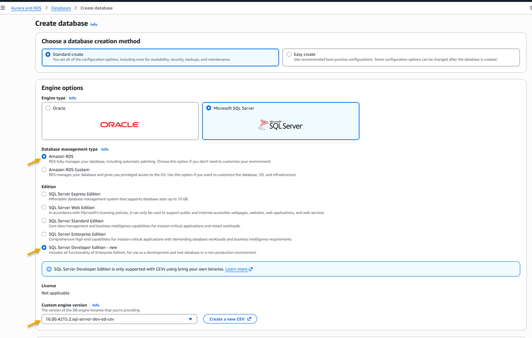
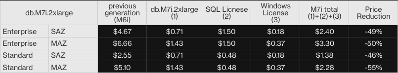
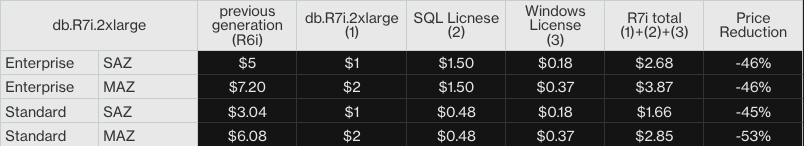
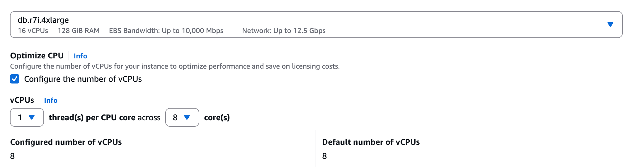
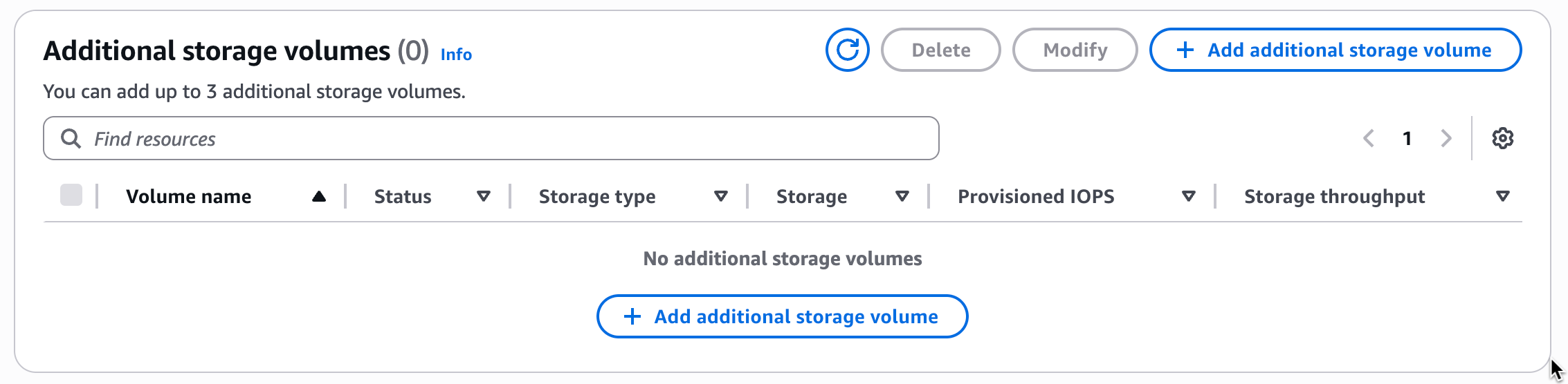
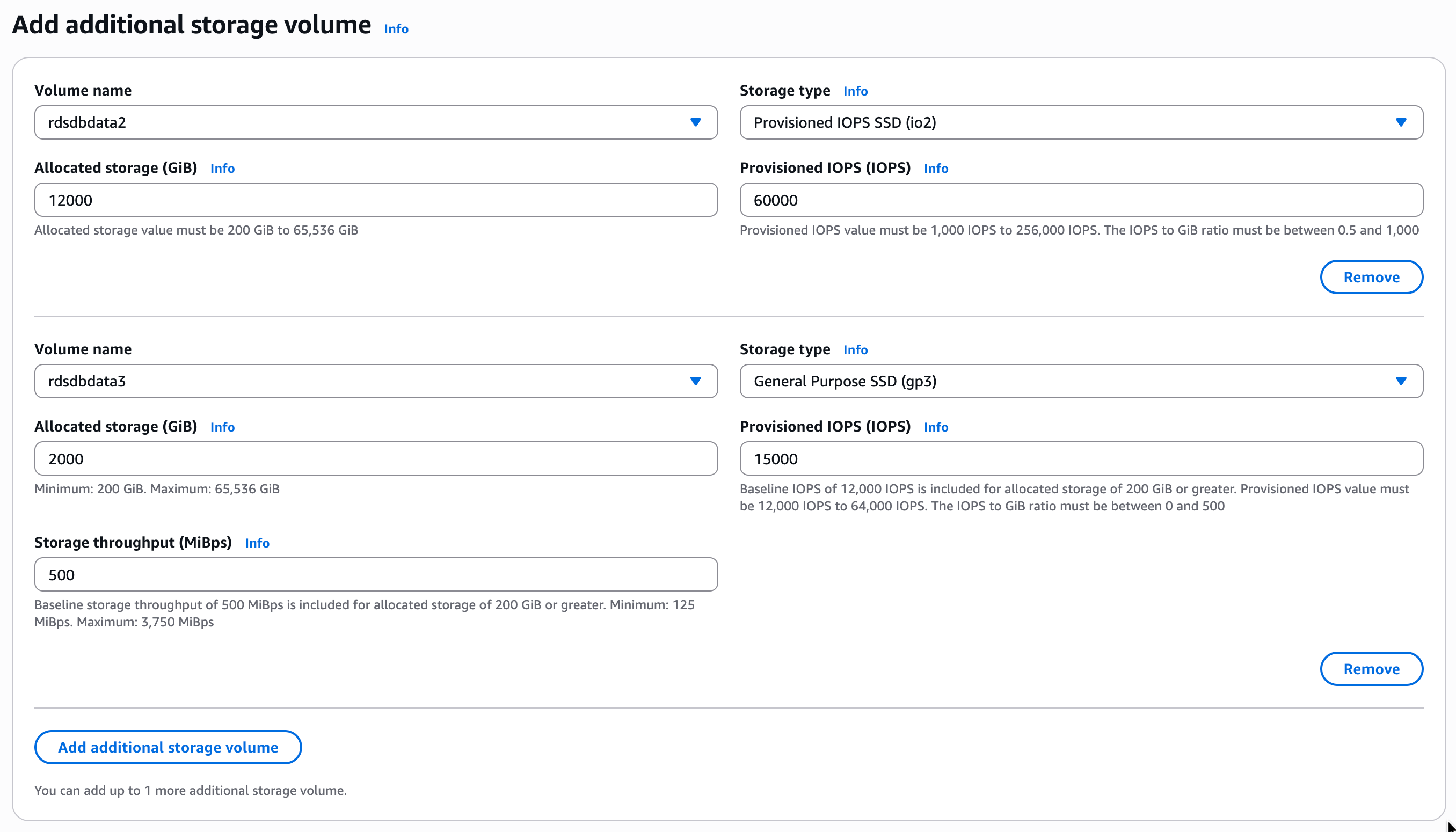
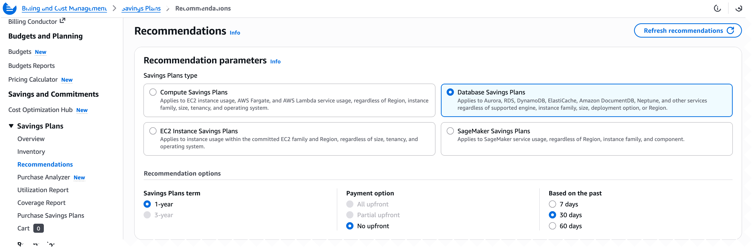
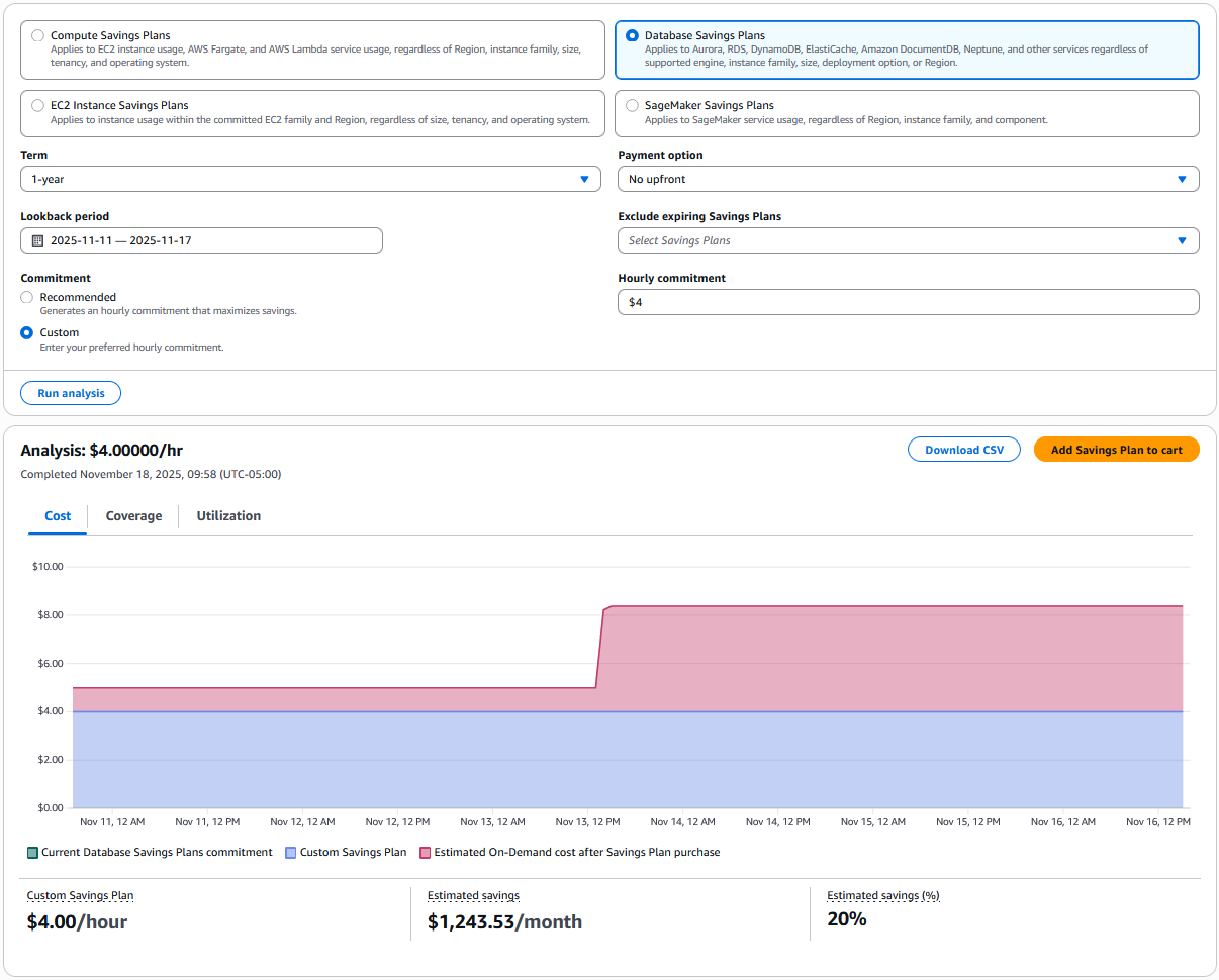
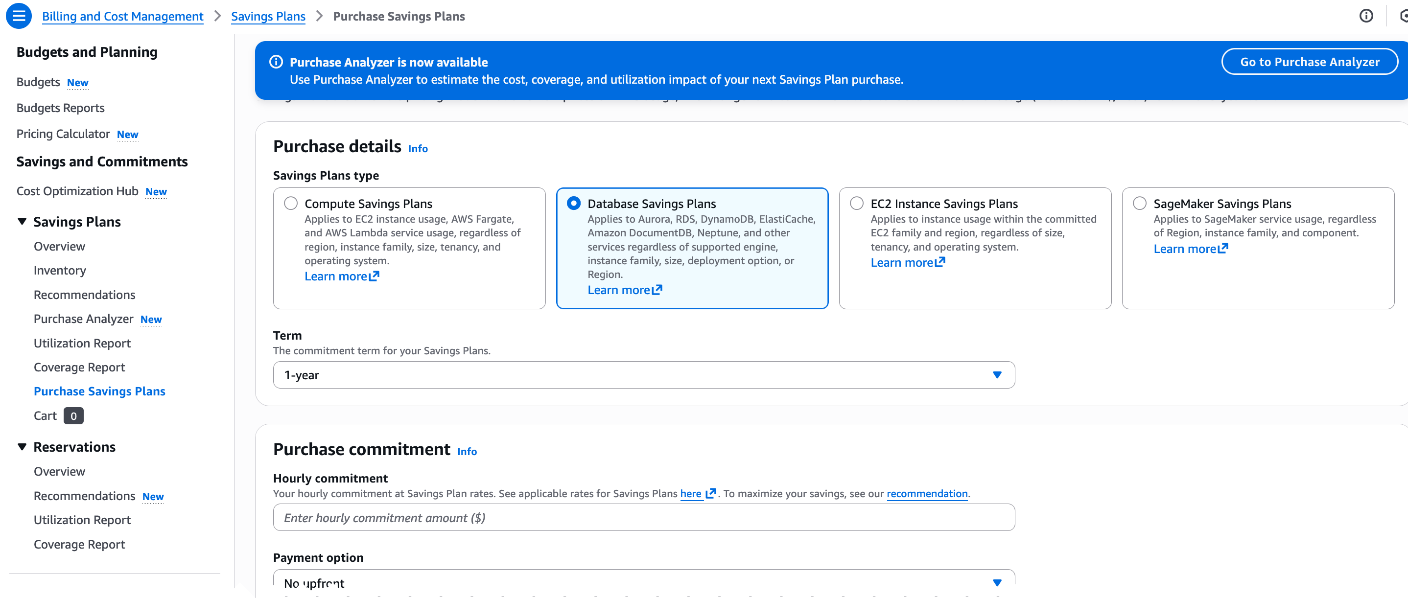
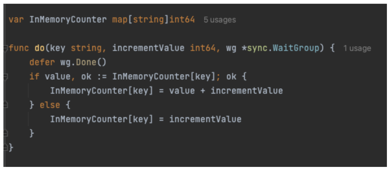
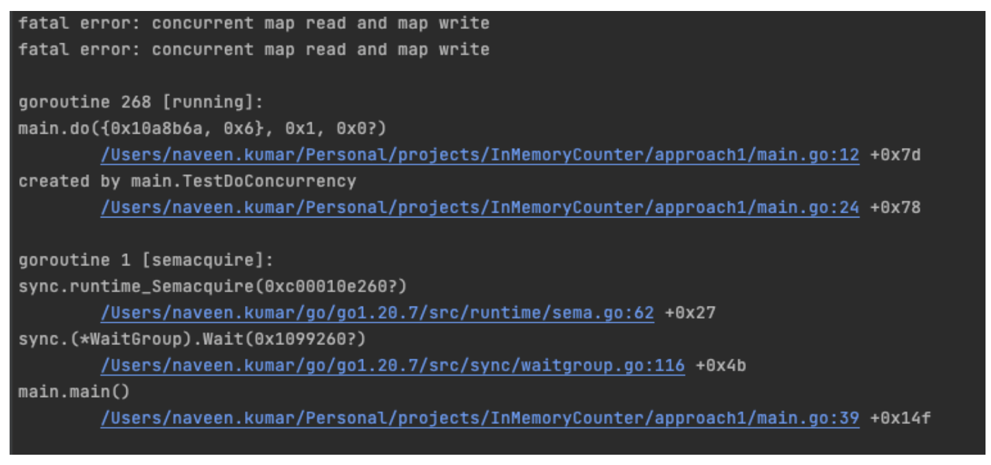
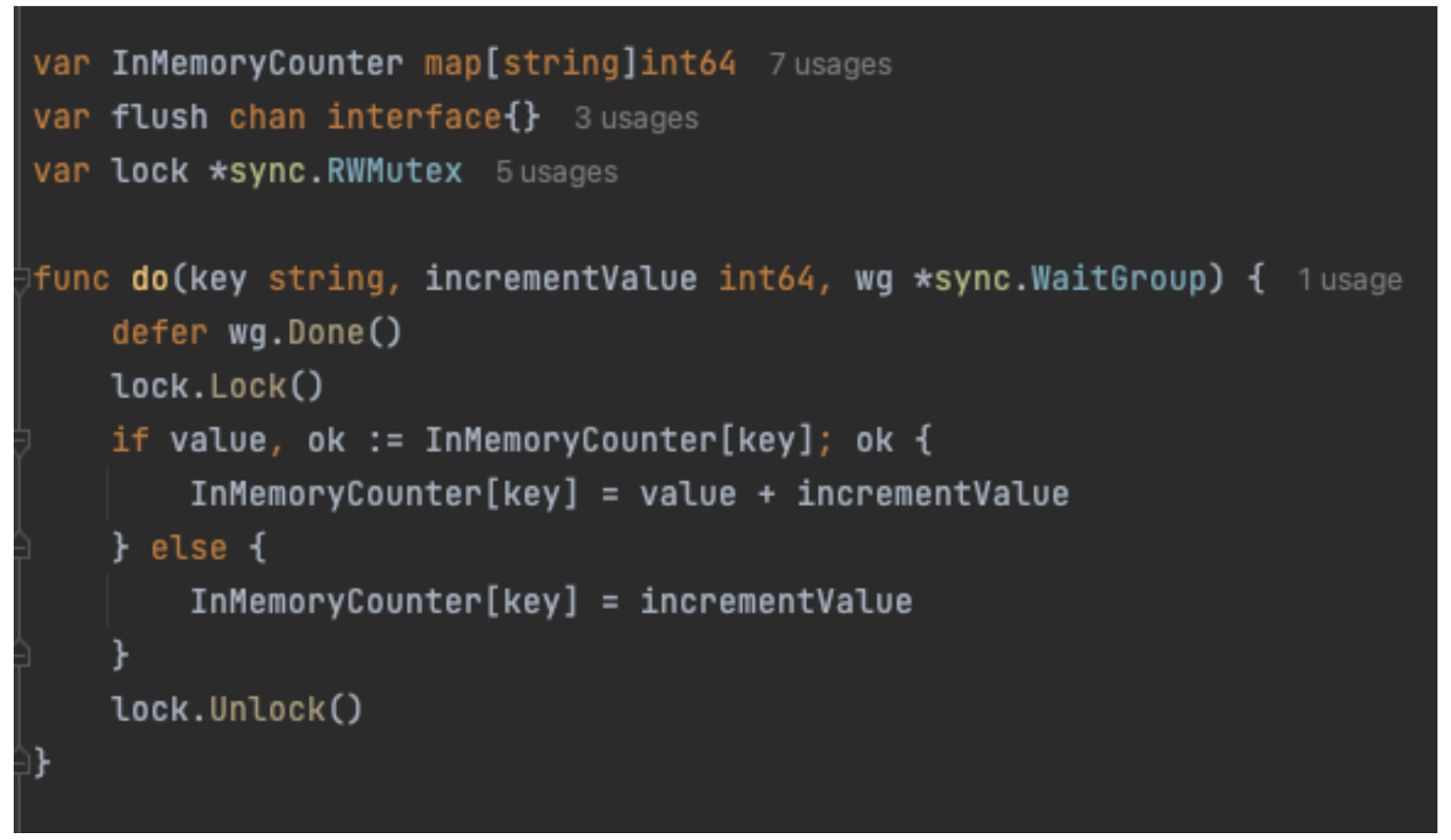
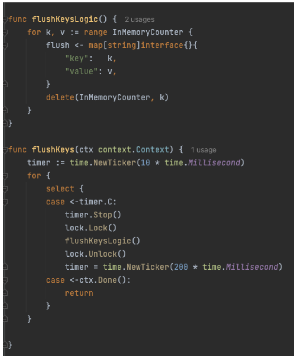
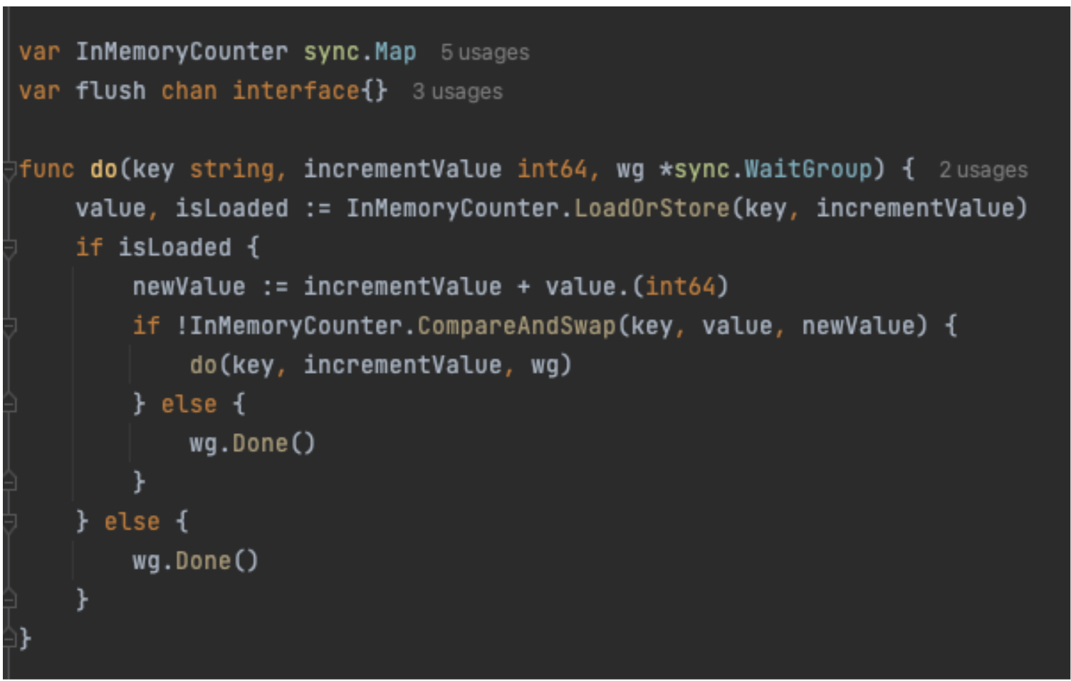
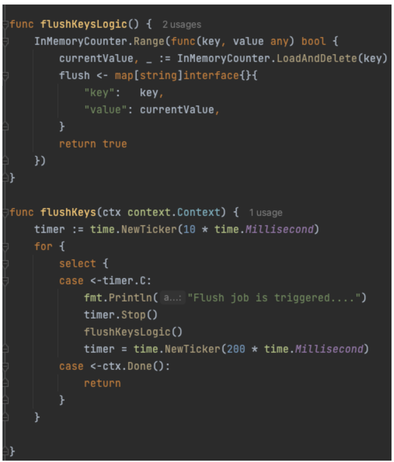

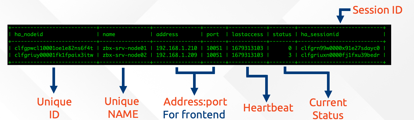
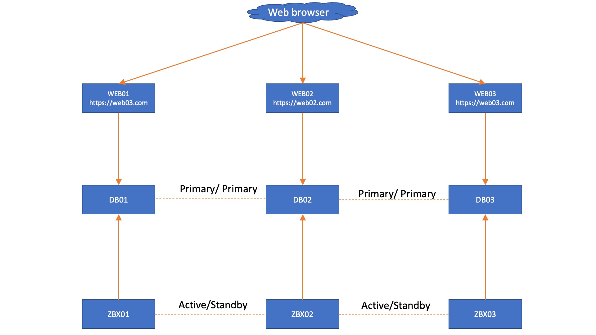
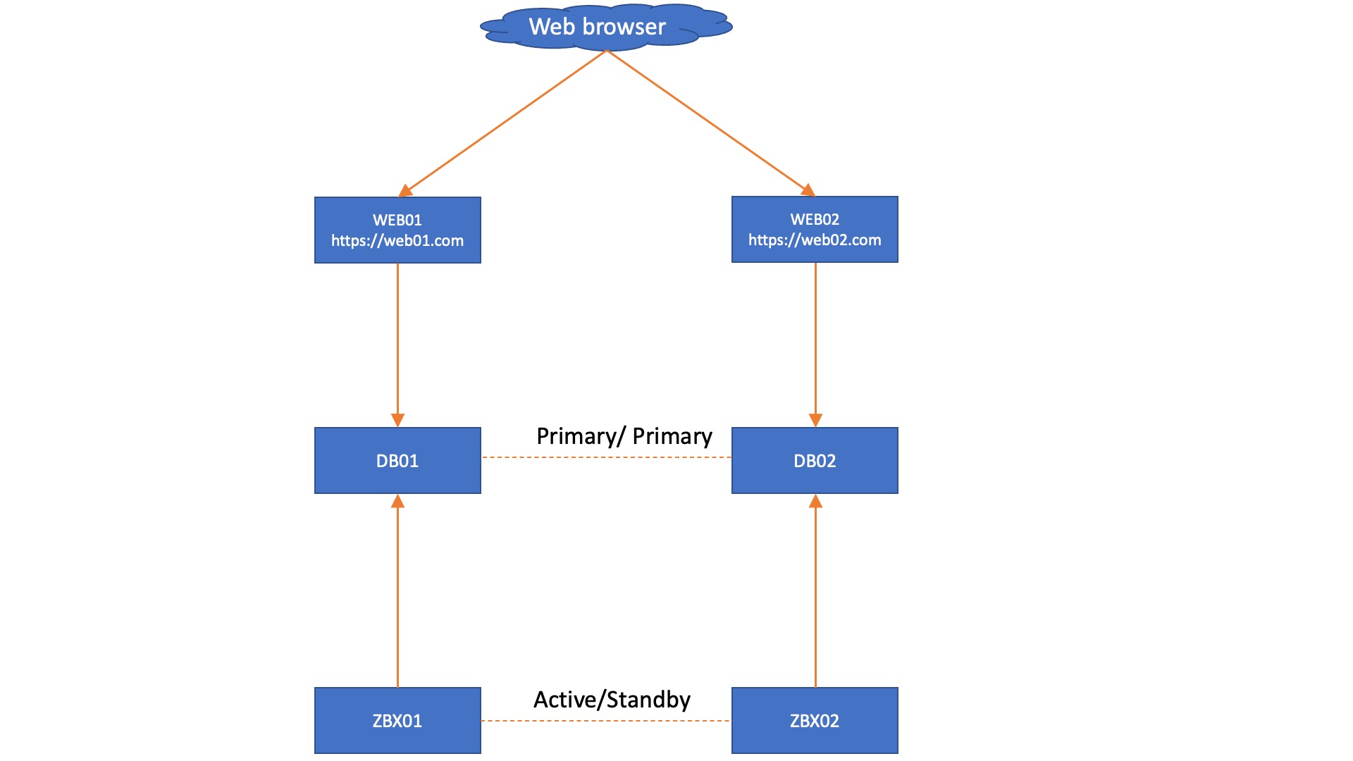
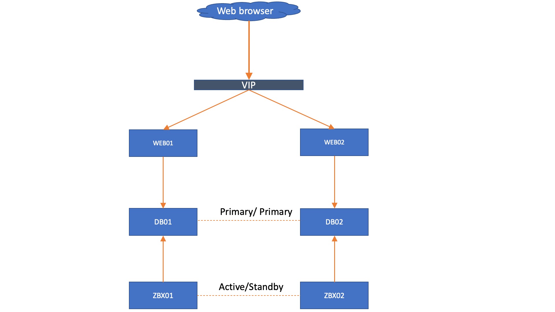

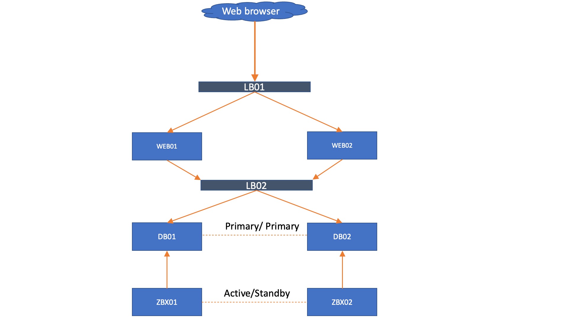


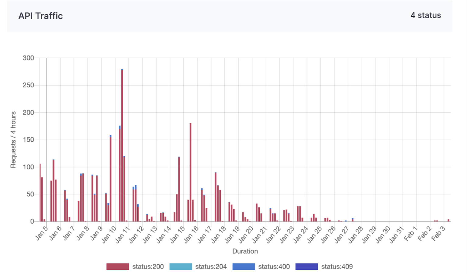
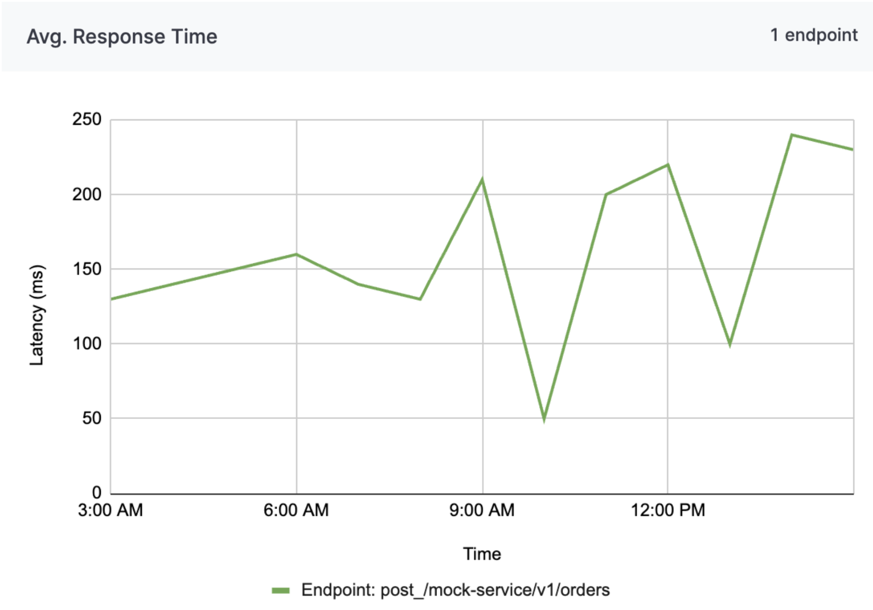
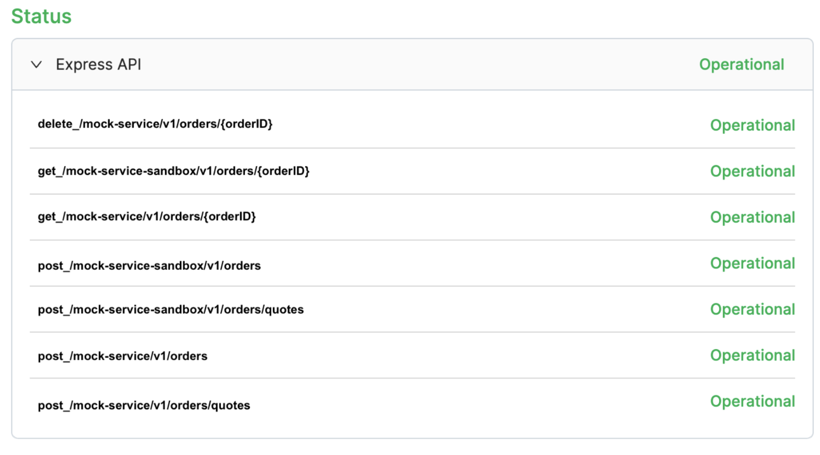
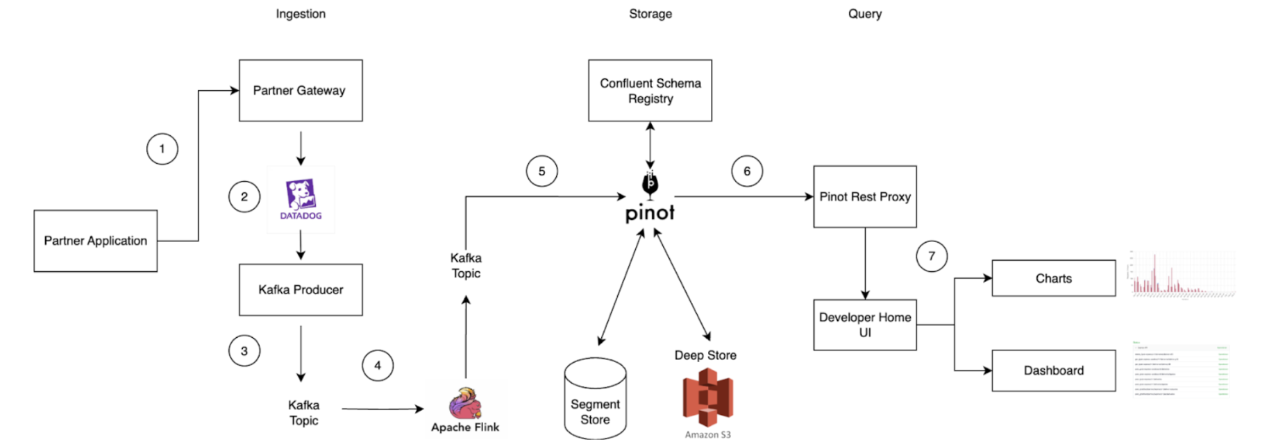
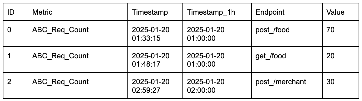
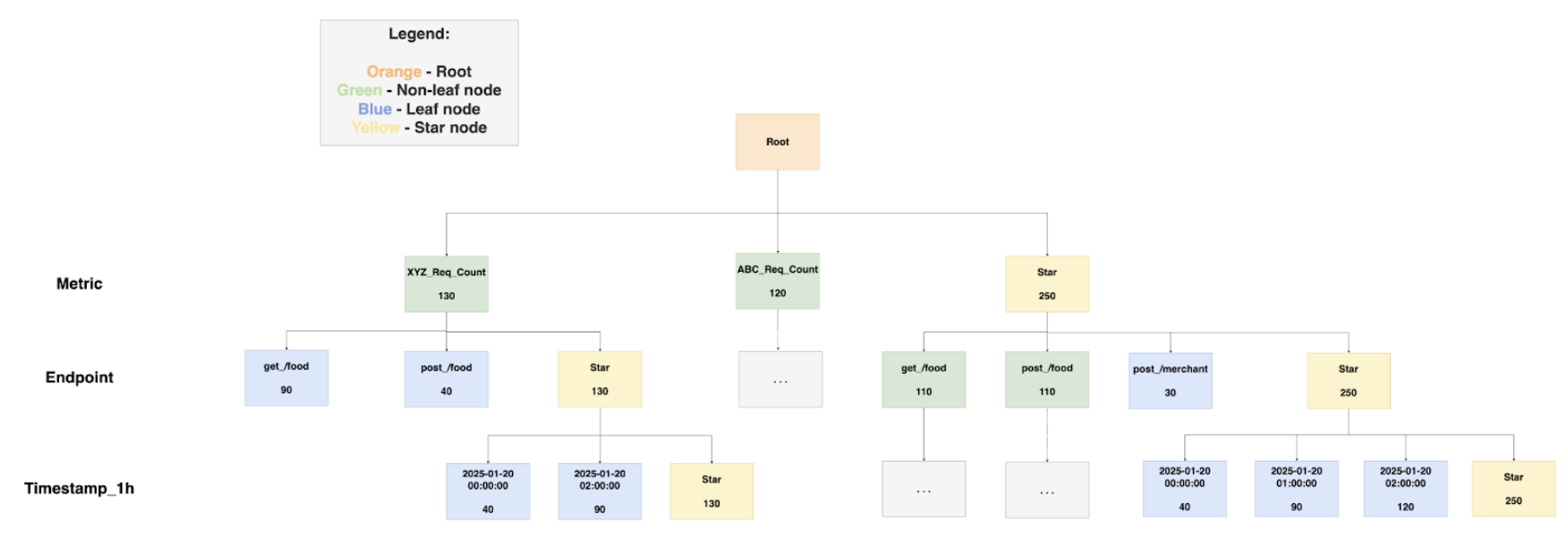
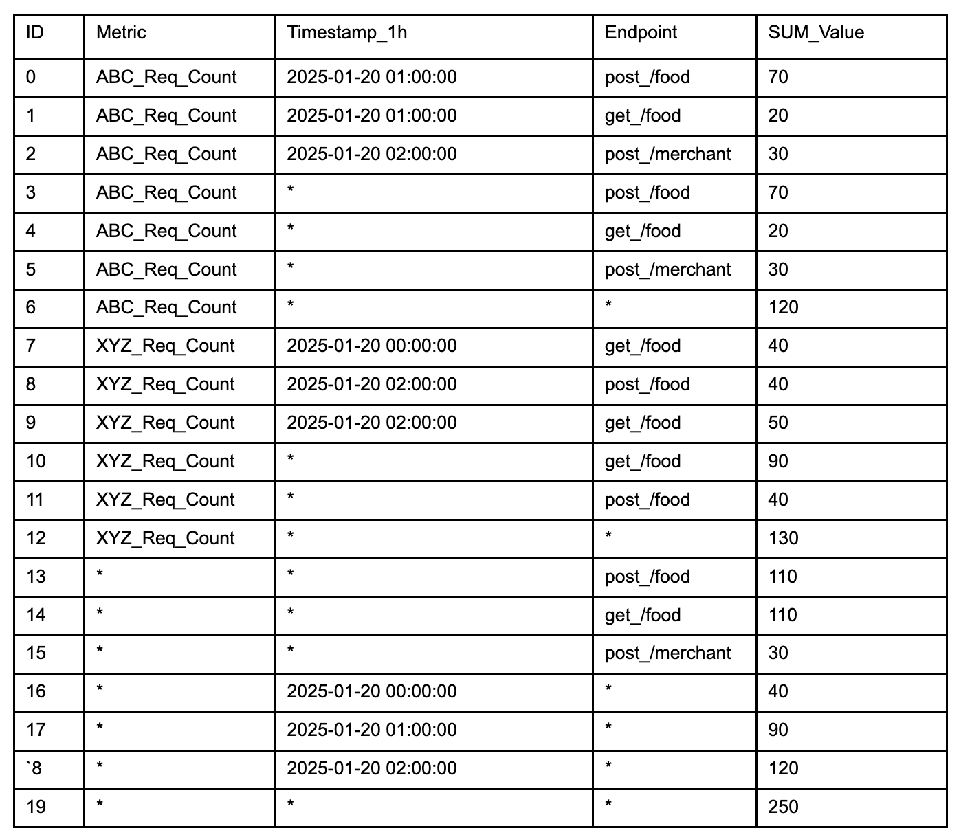
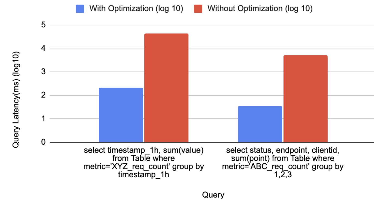
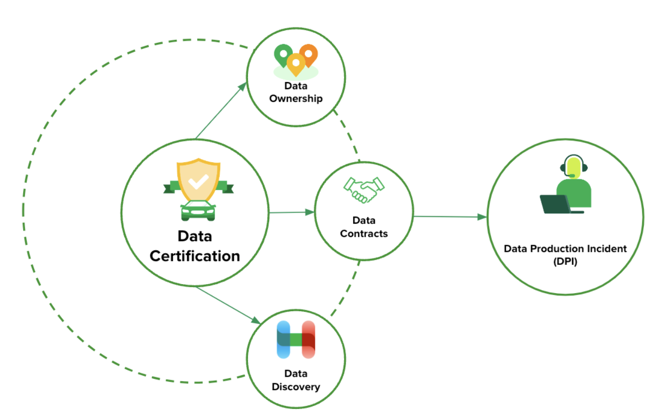

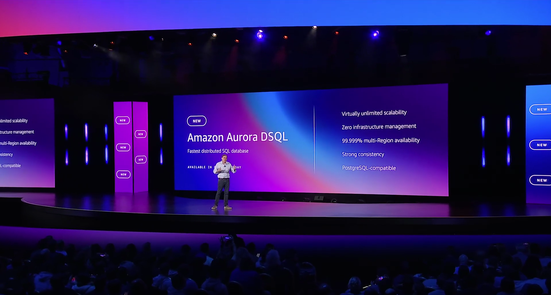

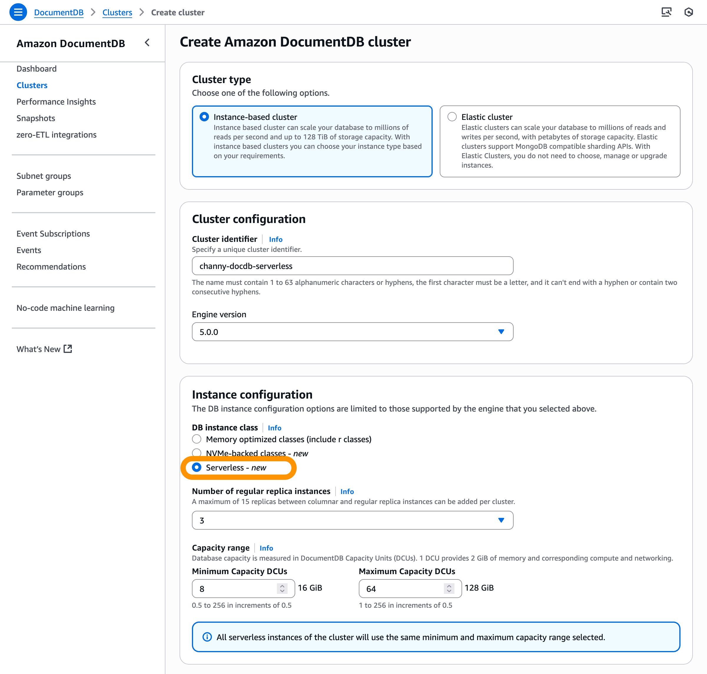
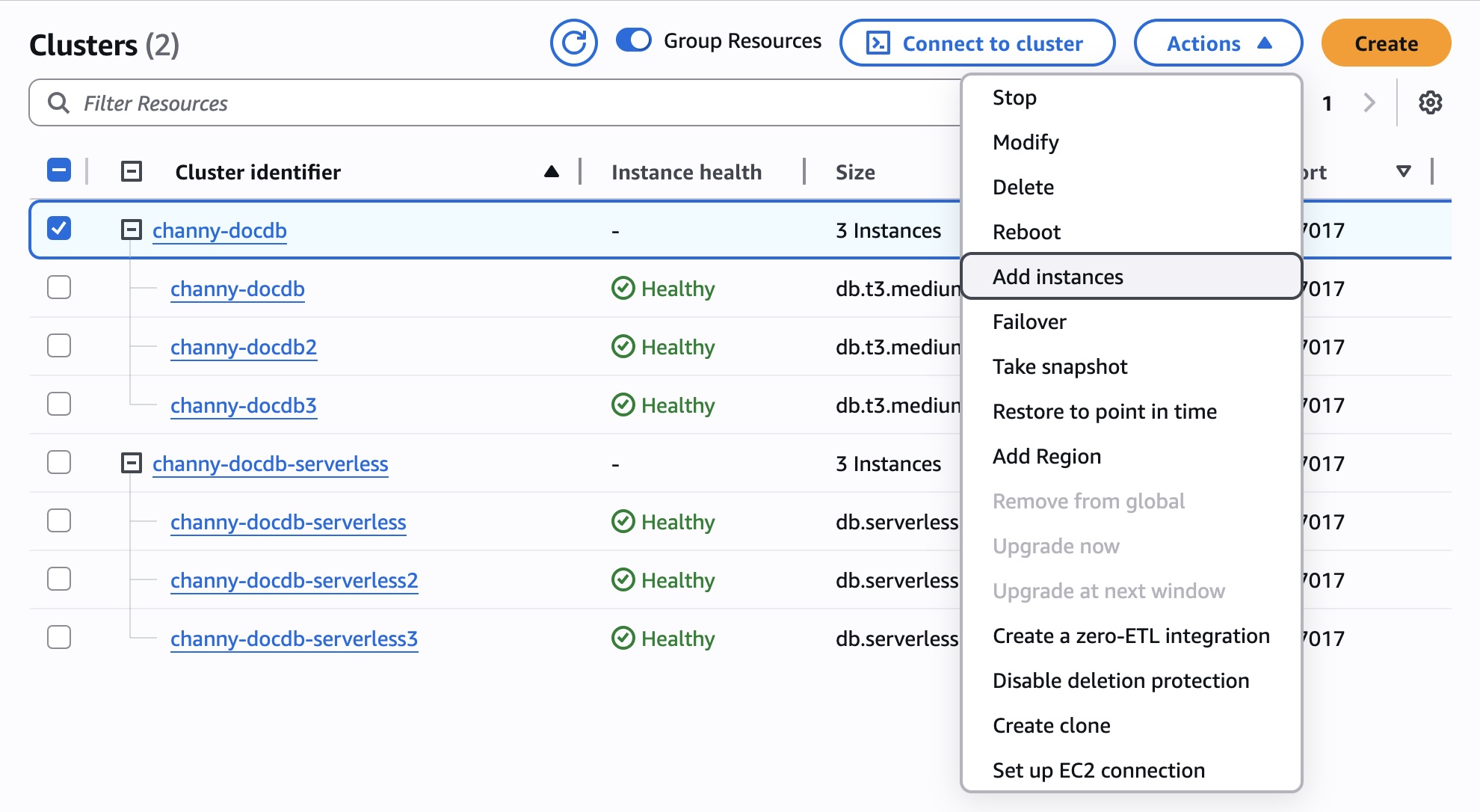
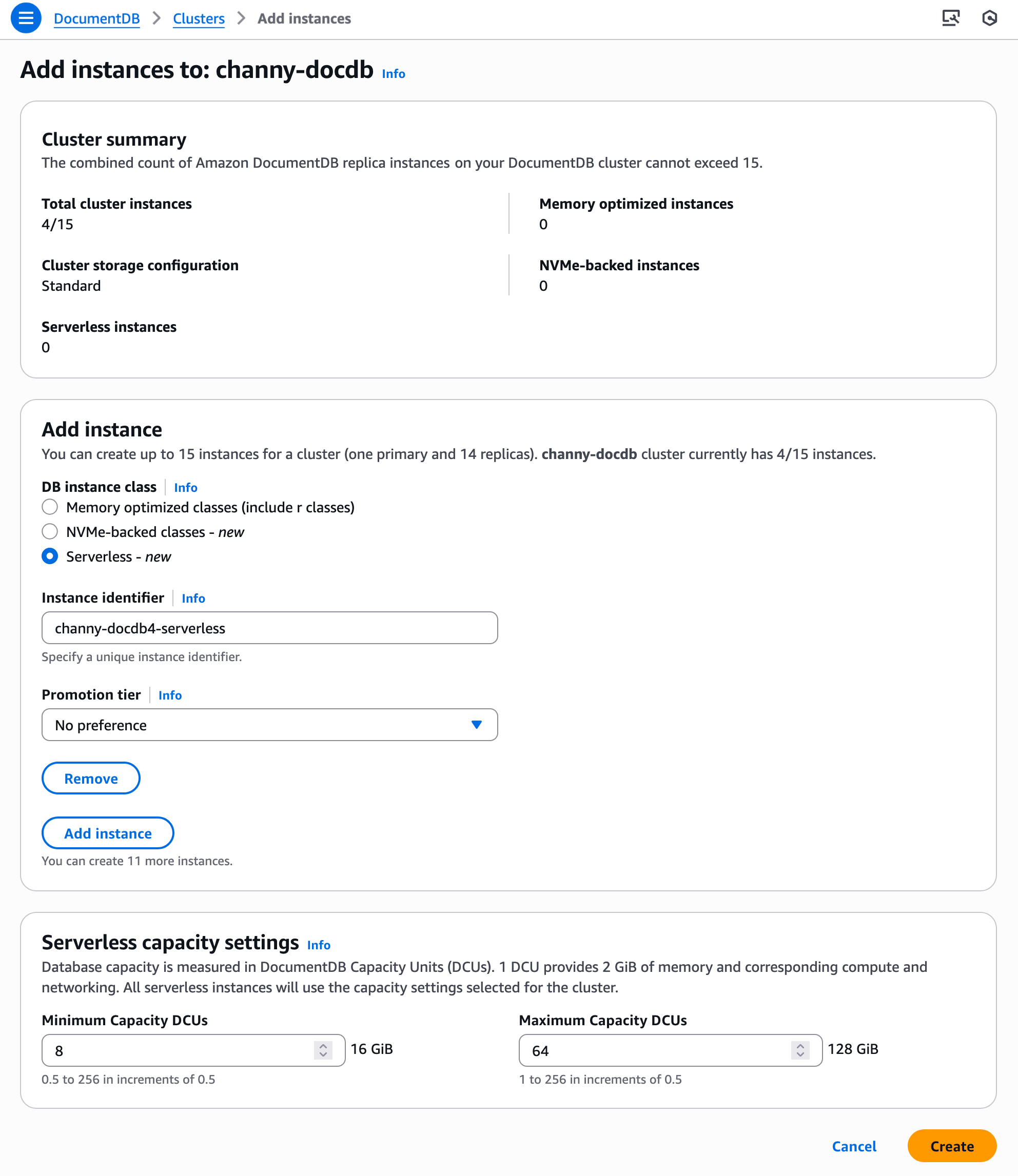
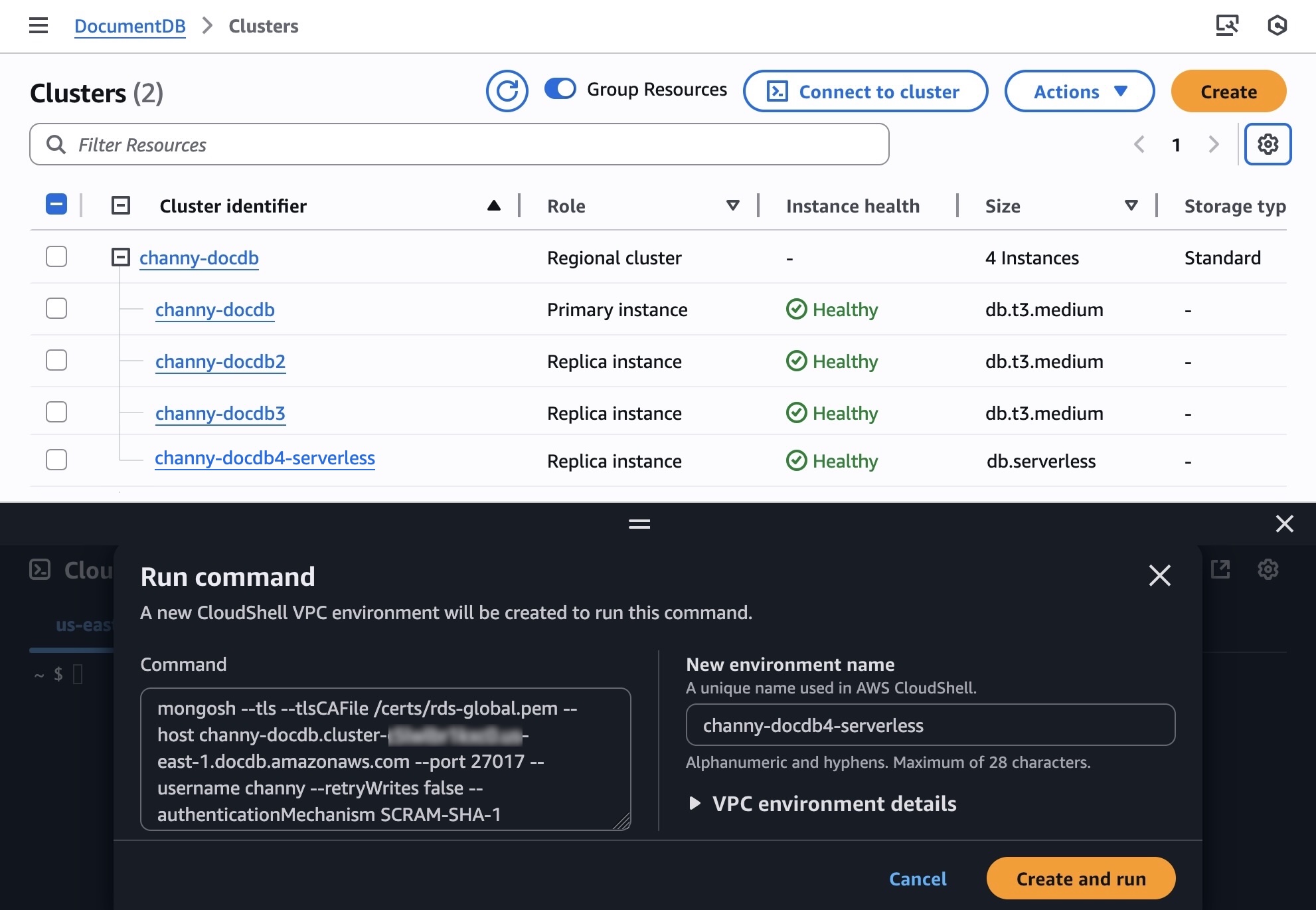
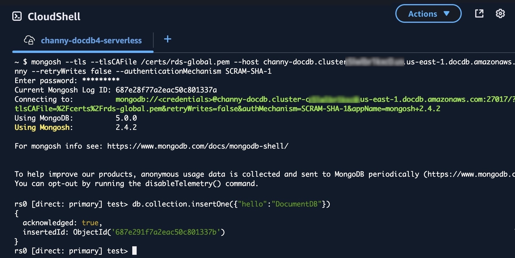
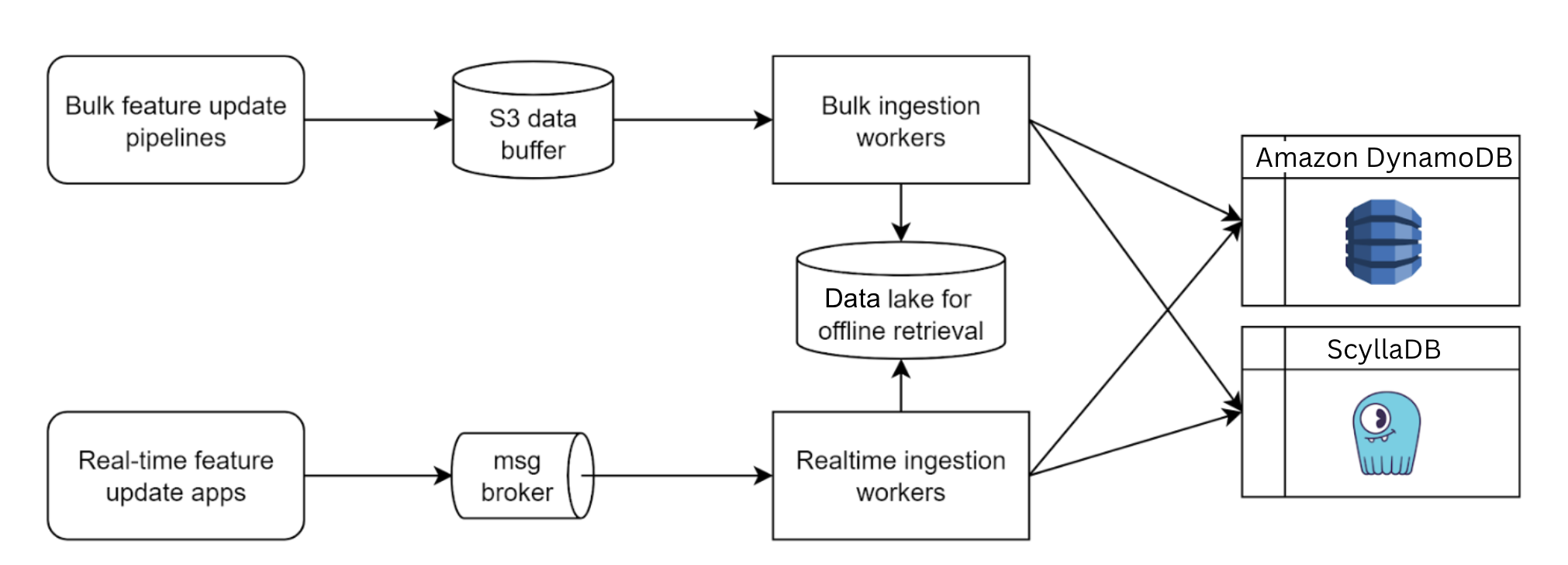
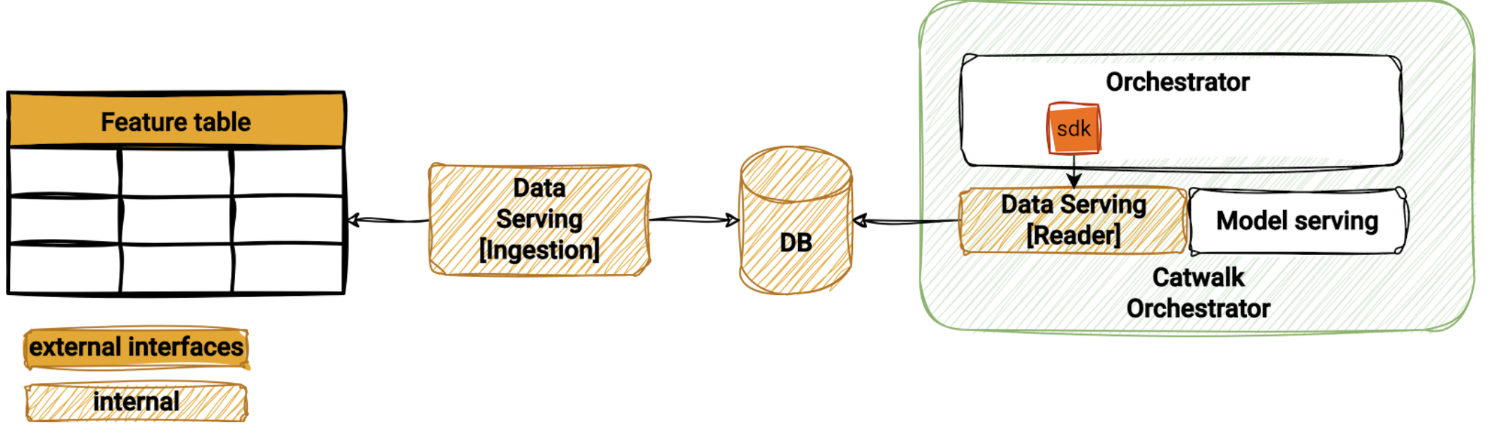
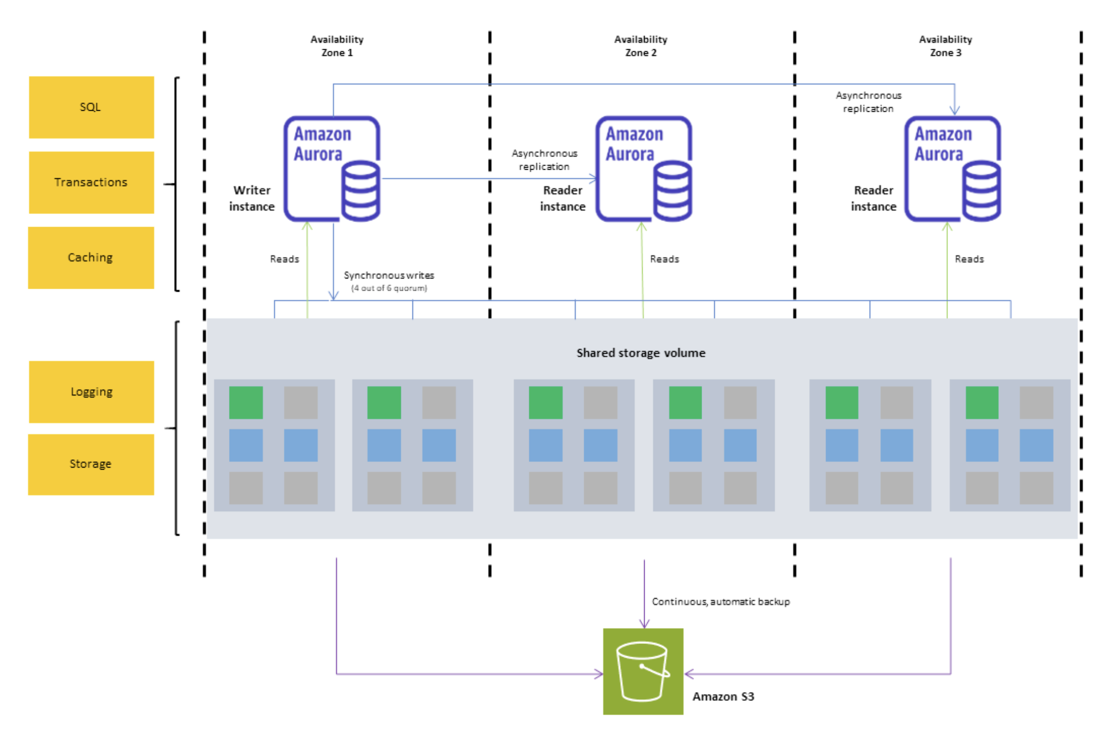


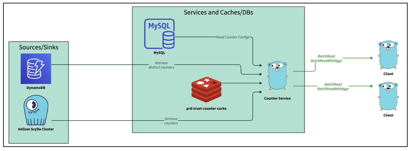
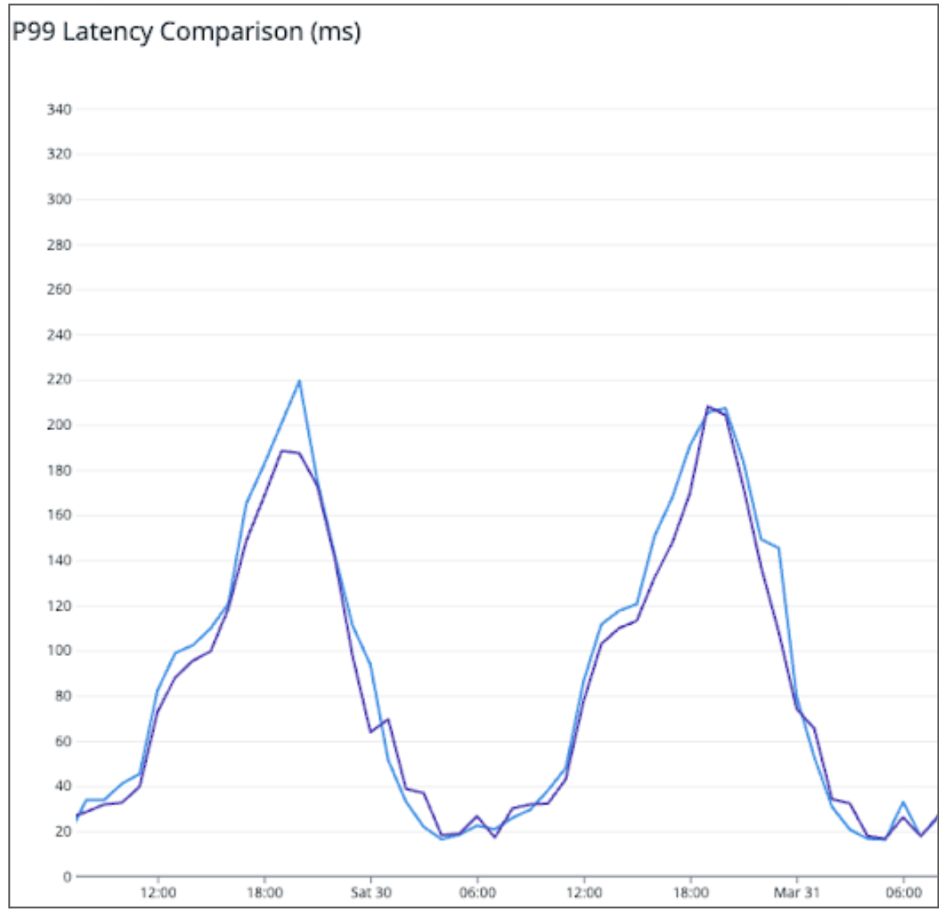
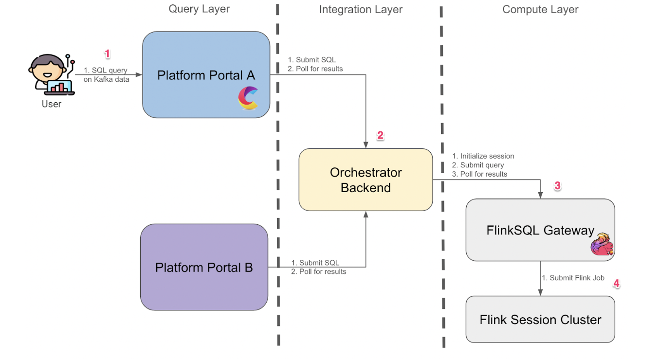
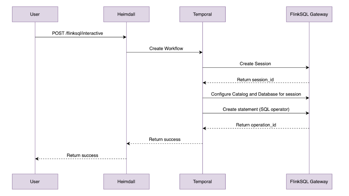
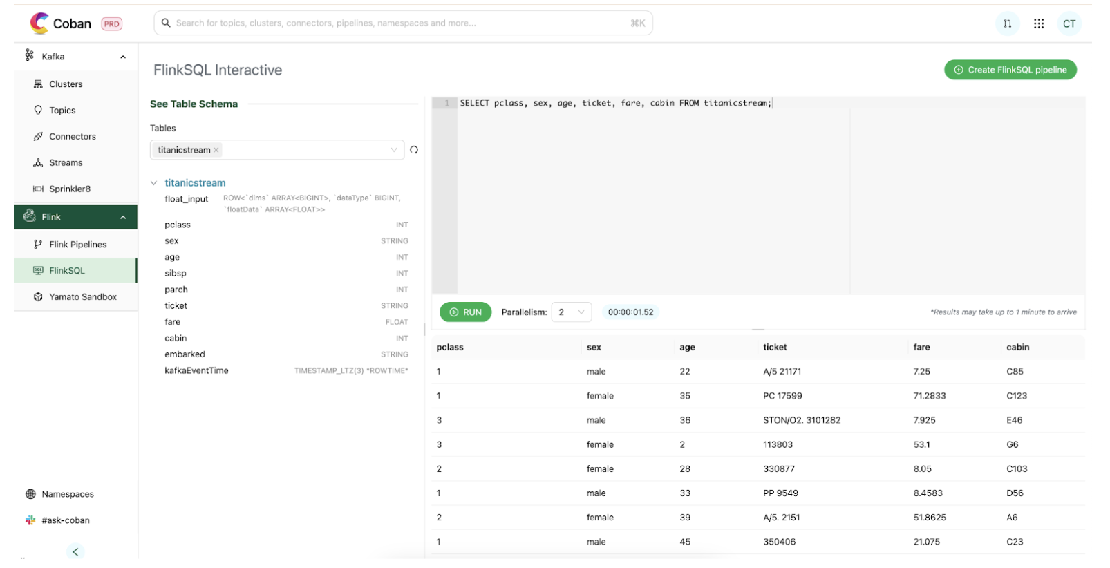
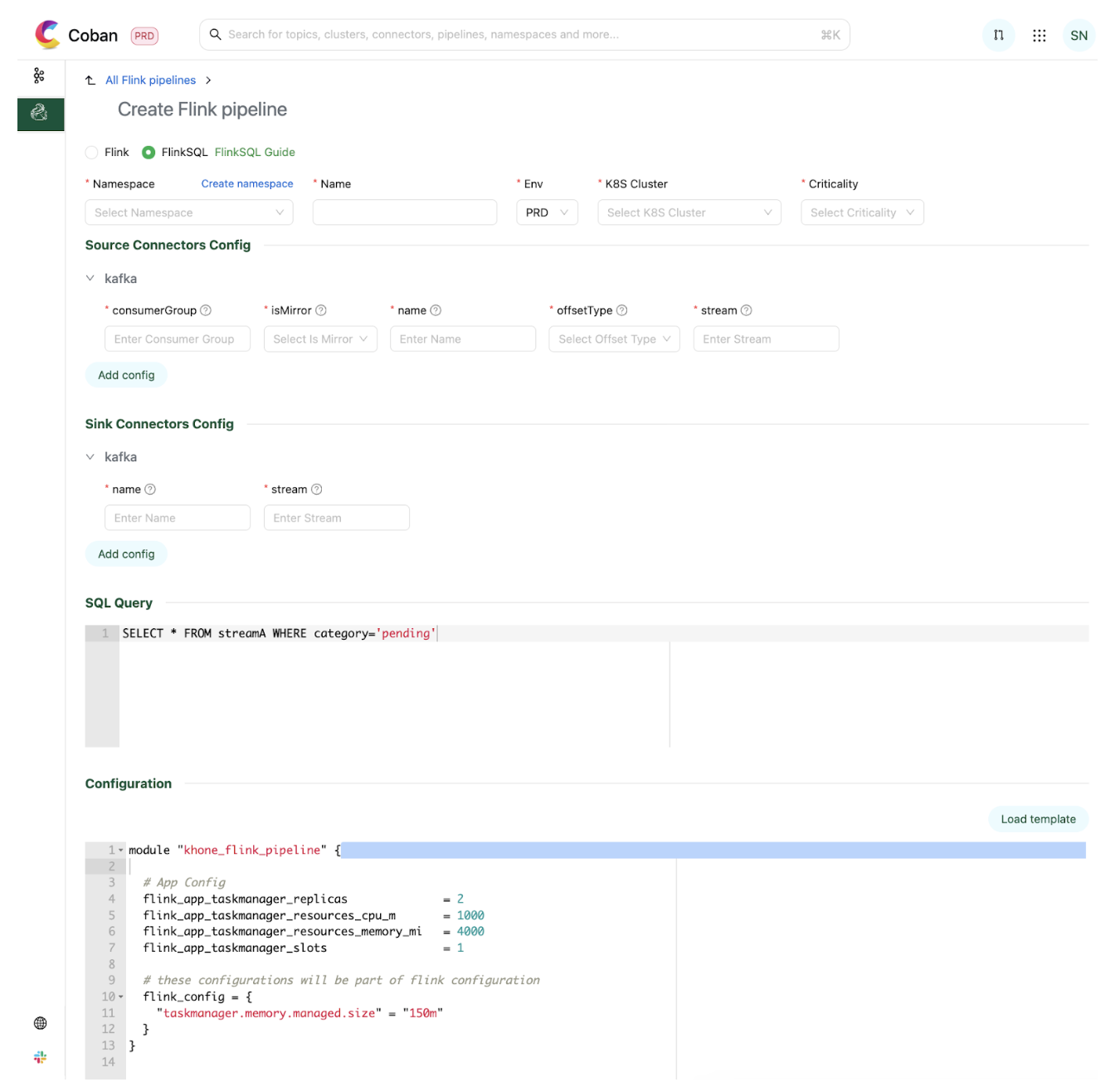
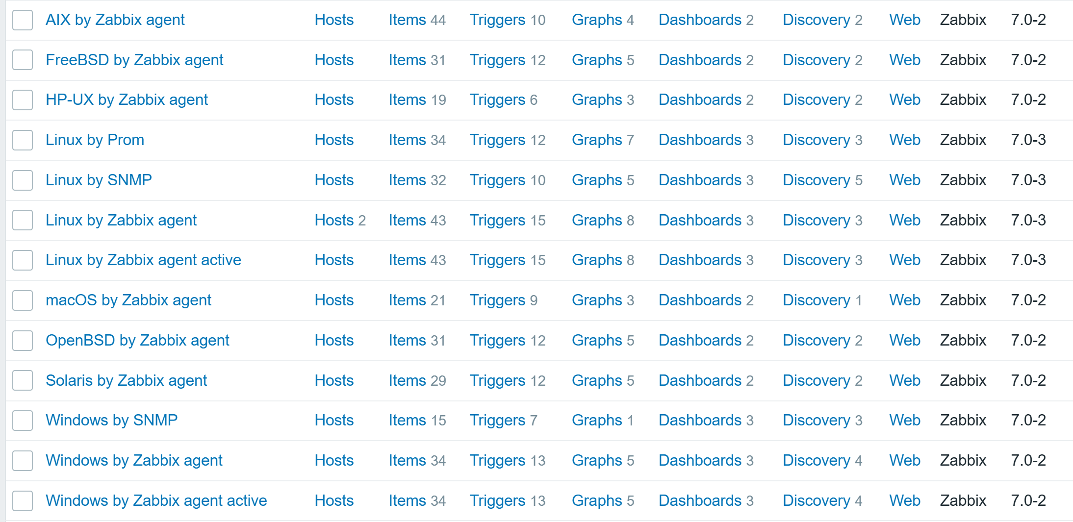
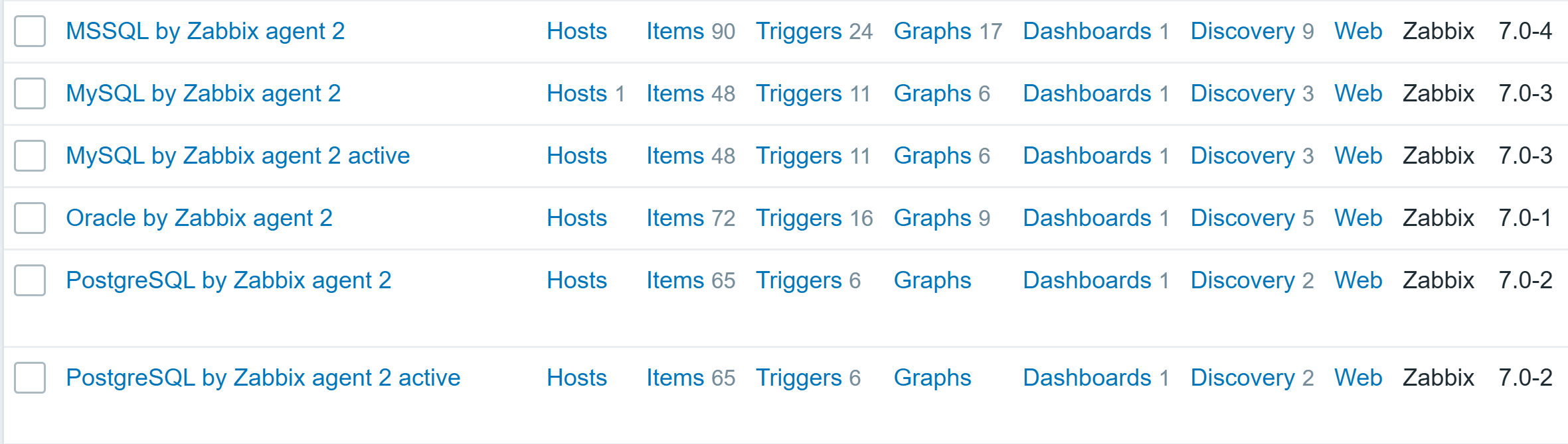
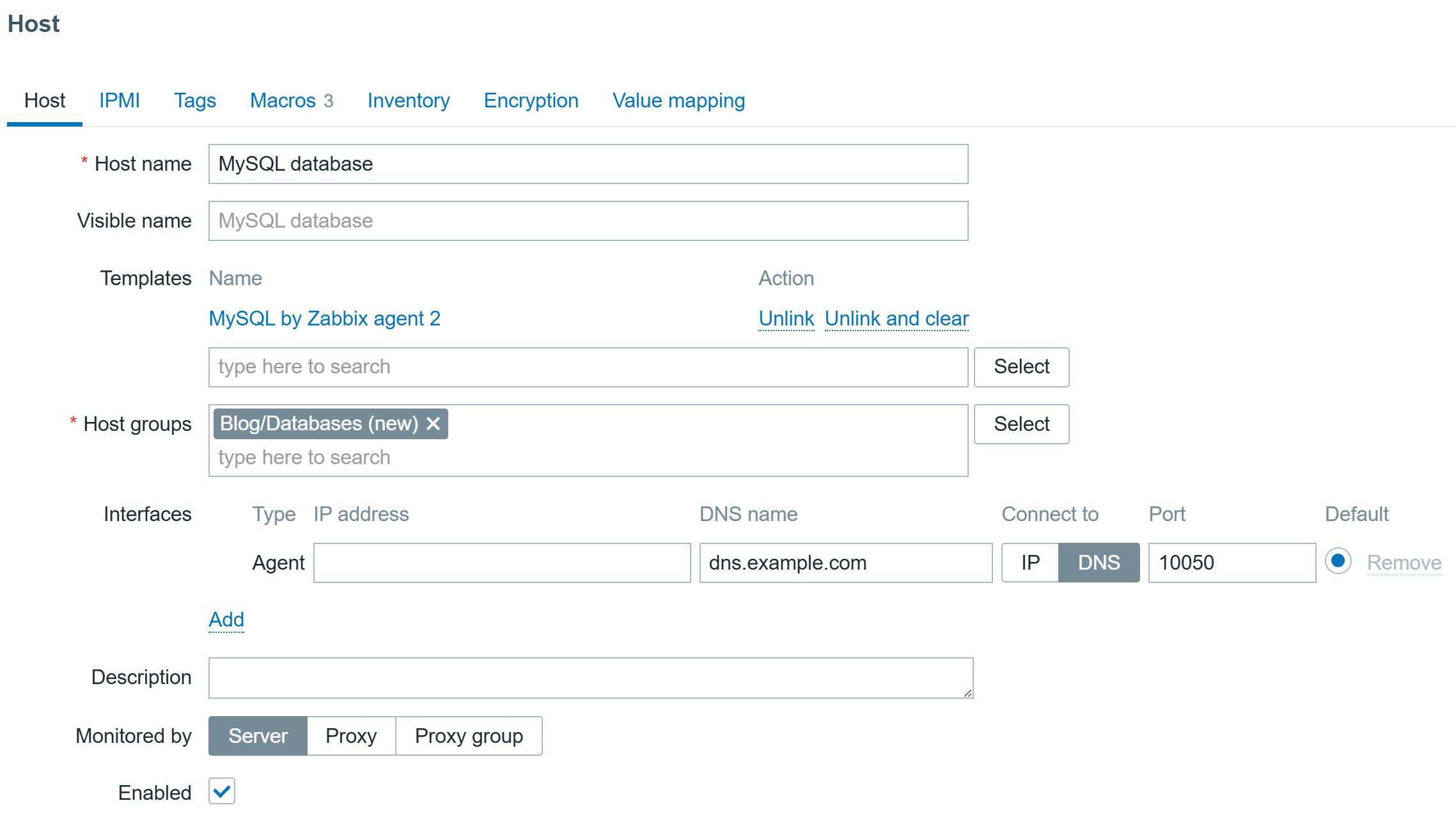
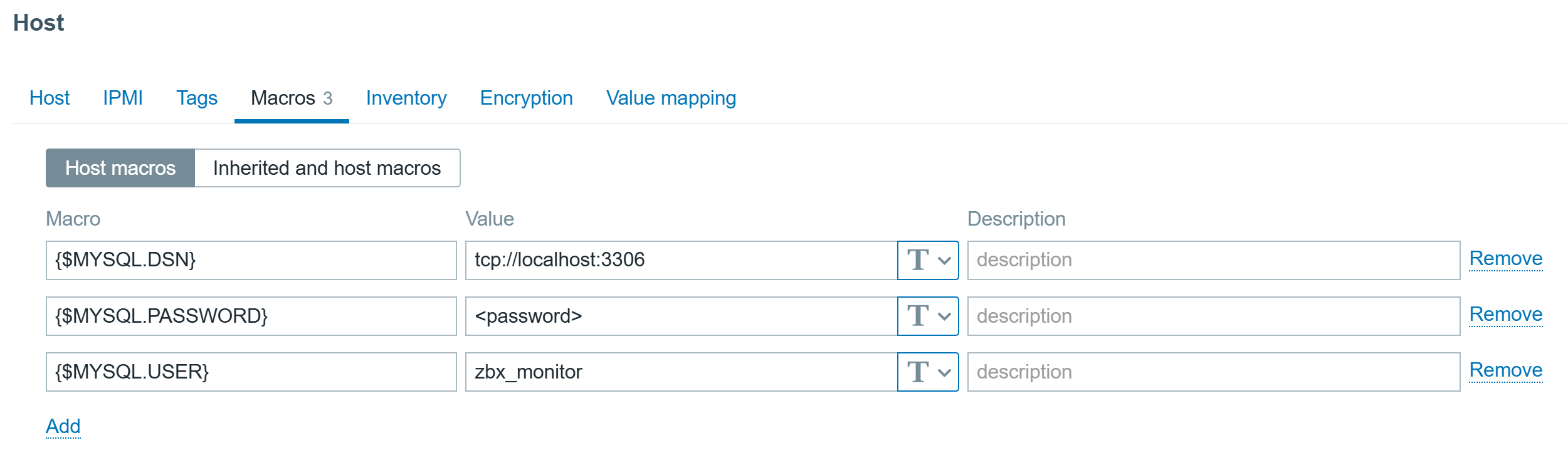
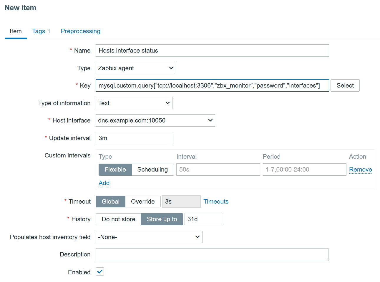
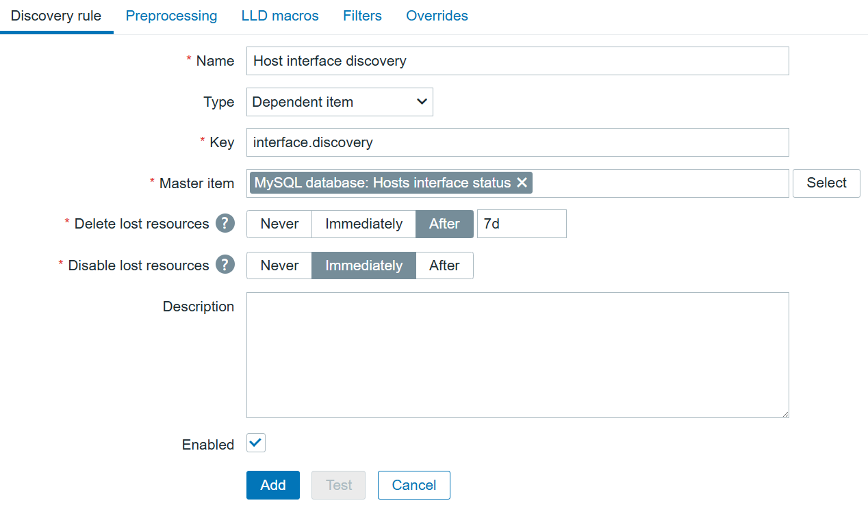
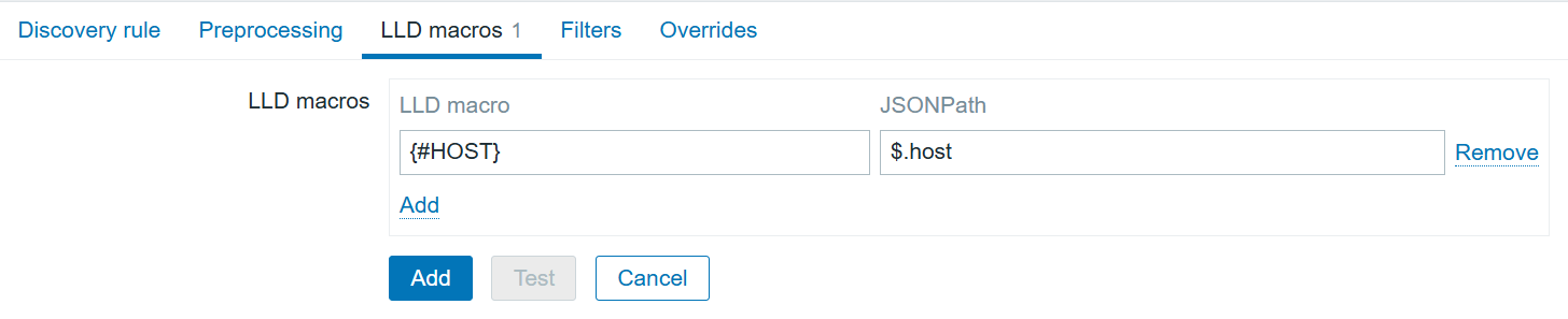
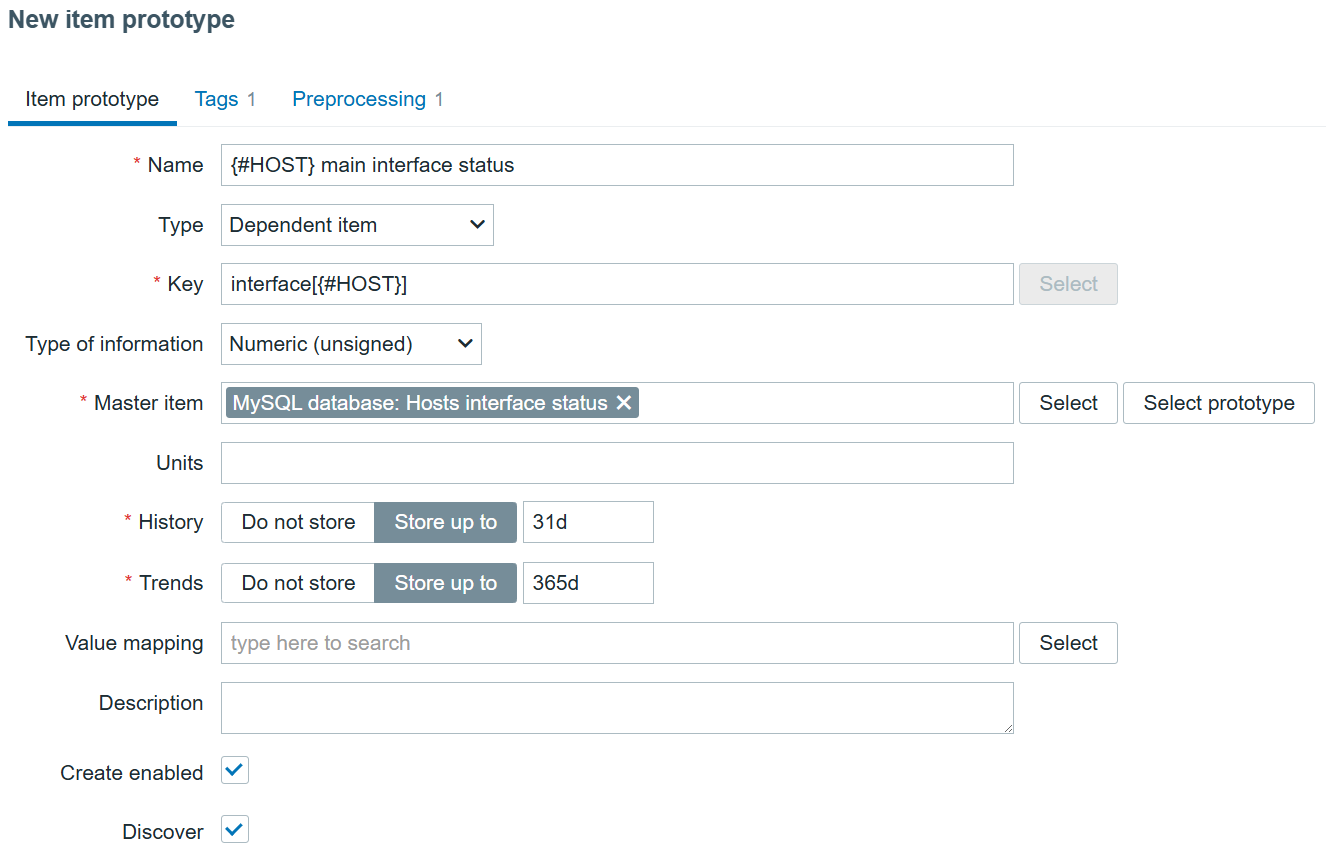
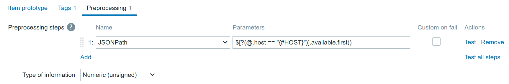
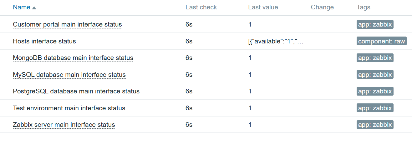
 When we introduced the