Post Syndicated from Abhilash Nagilla original https://aws.amazon.com/blogs/big-data/convert-oracle-xml-blob-data-to-json-using-amazon-emr-and-load-to-amazon-redshift/
In legacy relational database management systems, data is stored in several complex data types, such XML, JSON, BLOB, or CLOB. This data might contain valuable information that is often difficult to transform into insights, so you might be looking for ways to load and use this data in a modern cloud data warehouse such as Amazon Redshift. One such example is migrating data from a legacy Oracle database with XML BLOB fields to Amazon Redshift, by performing preprocessing and conversion of XML to JSON using Amazon EMR. In this post, we describe a solution architecture for this use case, and show you how to implement the code to handle the XML conversion.
Solution overview
The first step in any data migration project is to capture and ingest the data from the source database. For this task, we use AWS Database Migration Service (AWS DMS), a service that helps you migrate databases to AWS quickly and securely. In this example, we use AWS DMS to extract data from an Oracle database with XML BLOB fields and stage the same data in Amazon Simple Storage Service (Amazon S3) in Apache Parquet format. Amazon S3 is an object storage service offering industry-leading scalability, data availability, security, and performance, and is the storage of choice for setting up data lakes on AWS.
After the data is ingested into an S3 staging bucket, we used Amazon EMR to run a Spark job to perform the conversion of XML fields to JSON fields, and the results are loaded in a curated S3 bucket. Amazon EMR runtime for Apache Spark can be over three times faster than clusters without EMR runtime, and has 100% API compatibility with standard Apache Spark. This improved performance means your workloads run faster and it saves you compute costs, without making any changes to your application.
Finally, transformed and curated data is loaded into Amazon Redshift tables using the COPY command. The Amazon Redshift table structure should match the number of columns and the column data types in the source file. Because we stored the data as a Parquet file, we specify the SERIALIZETOJSON option in the COPY command. This allows us to load complex types, such as structure and array, in a column defined as SUPER data type in the table.
The following architecture diagram shows the end-to-end workflow.

In detail, AWS DMS migrates data from the source database tables into Amazon S3, in Parquet format. Apache Spark on Amazon EMR reads the raw data, transforms the XML data type into JSON, and saves the data to the curated S3 bucket. In our code, we used an open-source library, called spark-xml, to parse and query the XML data.
In the rest of this post, we assume that the AWS DMS tasks have already run and created the source Parquet files in the S3 staging bucket. If you want to set up AWS DMS to read from an Oracle database with LOB fields, refer to Effectively migrating LOB data to Amazon S3 from Amazon RDS for Oracle with AWS DMS or watch the video Migrate Oracle to S3 Data lake via AWS DMS.
Prerequisites
If you want to follow along with the examples in this post using your AWS account, we provide an AWS CloudFormation template you can launch by choosing Launch Stack:
![]()
Provide a stack name and leave the default settings for everything else. Wait for the stack to display Create Complete (this should only take a few minutes) before moving on to the other sections.
The template creates the following resources:
- A virtual private cloud (VPC) with two private subnets that have routes to an Amazon S3 VPC endpoint
- The S3 bucket
{stackname}-s3bucket-{xxx}, which contains the following folders:libs– Contains the JAR file to add to the notebooknotebooks– Contains the notebook to interactively test the codedata– Contains the sample data
- An Amazon Redshift cluster, in one of the two private subnets, with a database named
rs_xml_dband a schema namedrs_xml - A secret (
rs_xml_db) in AWS Secrets Manager - An EMR cluster
The CloudFormation template shared in this post is purely for demonstration purposes only. Please conduct your own security review and incorporate best practices prior to any production deployment using artifacts from the post.
Finally, some basic knowledge of Python and Spark DataFrames can help you review the transformation code, but isn’t mandatory to complete the example.
Understanding the sample data
In this post, we use college students’ course and subjects sample data that we created. In the source system, data consists of flat structure fields, like course_id and course_name, and an XML field that includes all the course material and subjects involved in the respective course. The following screenshot is an example of the source data, which is staged in an S3 bucket as a prerequisite step.

We can observe that the column study_material_info is an XML type field and contains nested XML tags in it. Let’s see how to convert this nested XML field to JSON in the subsequent steps.
Run a Spark job in Amazon EMR to transform the XML fields in the raw data to JSON
In this step, we use an Amazon EMR notebook, which is a managed environment to create and open Jupyter Notebook and JupyterLab interfaces. It enables you to interactively analyze and visualize data, collaborate with peers, and build applications using Apache Spark on EMR clusters. To open the notebook, follow these steps:
- On the Amazon S3 console, navigate to the bucket you created as a prerequisite step.
- Download the file in the notebooks folder.

- On the Amazon EMR console, choose Notebooks in the navigation pane.
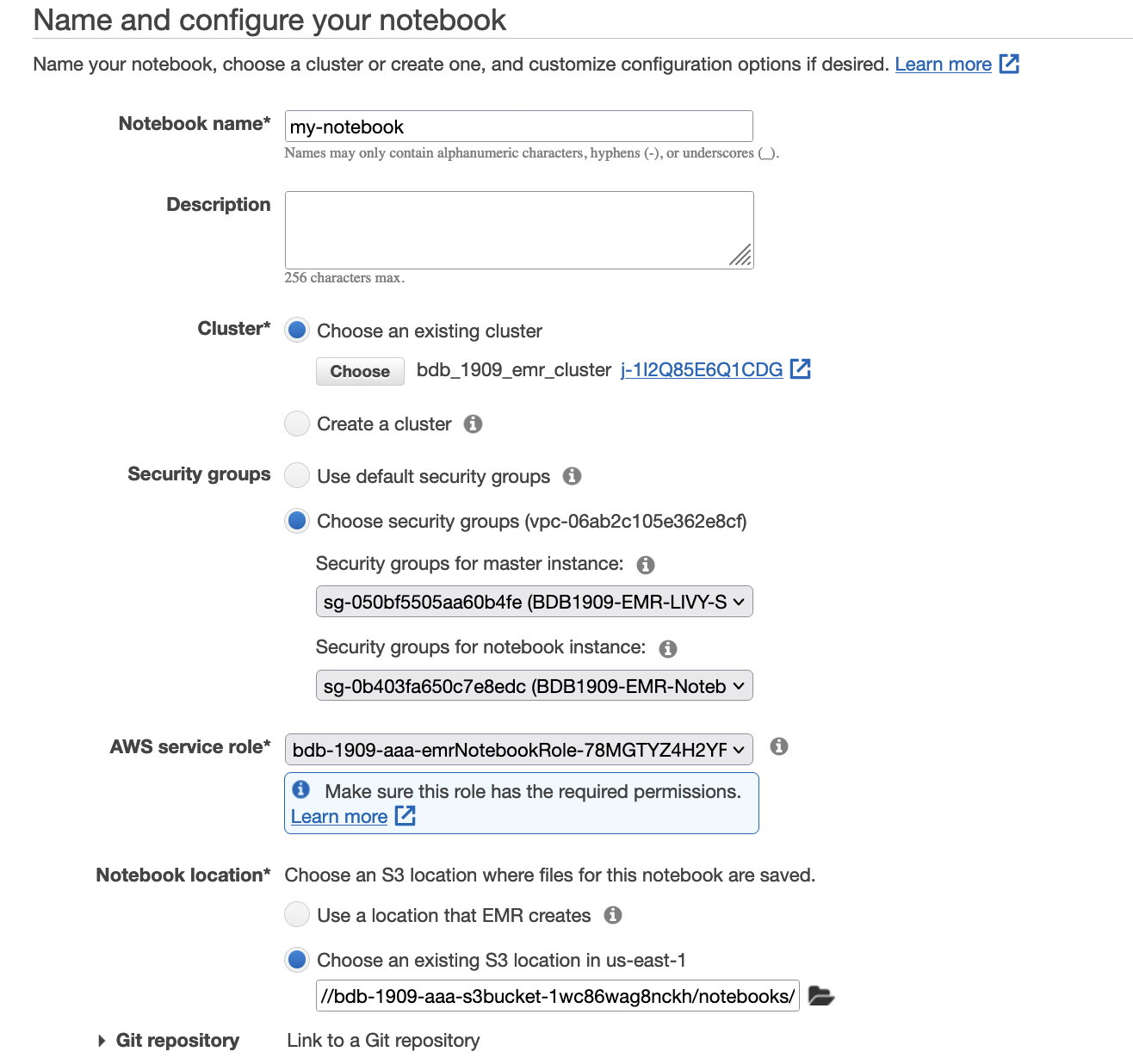
- Choose Create notebook.
- For Notebook name, enter a name.
- For Cluster, select Choose an existing cluster.
- Select the cluster you created as a prerequisite.

- For Security Groups, choose
BDB1909-EMR-LIVY-SGandBDB1909-EMR-Notebook-SG - For AWS Service Role, choose the role
bdb1909-emrNotebookRole-{xxx}. - For Notebook location, specify the S3 path in the notebooks folder (
s3://{stackname}-s3bucket-xxx}/notebooks/). - Choose Create notebook.

- When the notebook is created, choose Open in JupyterLab.

- Upload the file you downloaded earlier.

- Open the new notebook.

The notebook should look as shown in the following screenshot, and it contains a script written in Scala.

- Run the first two cells to configure Apache Spark with the open-source spark-xml library and import the needed modules.The
spark-xmlpackage allows reading XML files in local or distributed file systems as Spark DataFrames. Although primarily used to convert (portions of) large XML documents into a DataFrame,spark-xmlcan also parse XML in a string-valued column in an existing DataFrame with thefrom_xmlfunction, in order to add it as a new column with parsed results as a struct. - To do so, in the third cell, we load the data from the Parquet file generated by AWS DMS into a DataFrame, then we extract the attribute that contains the XML code (
STUDY_MATERIAL_INFO) and map it to a string variable namepayloadSchema. - We can now use the
payloadSchemain thefrom_xmlfunction to convert the fieldSTUDY_MATERIAL_INFOinto a struct data type and added it as a column namedcourse_materialin a new DataFrameparsed. - Finally, we can drop the original field and write the parsed DataFrame to our
curatedzone in Amazon S3.


Due to the structure differences between DataFrame and XML, there are some conversion rules from XML data to DataFrame and from DataFrame to XML data. More details and documentation are available XML Data Source for Apache Spark.
When we convert from XML to DataFrame, attributes are converted as fields with the heading prefix attributePrefix (underscore (_) is the default). For example, see the following code:
It produces the following schema:
Next, we have a value in an element that has no child elements but attributes. The value is put in a separate field, valueTag. See the following code:
It produces the following schema, and the tag lang is converted into the _lang field inside the DataFrame:
Copy curated data into Amazon Redshift and query tables seamlessly
Because our semi-structured nested dataset is already written in the S3 bucket as Apache Parquet formatted files, we can use the COPY command with the SERIALIZETOJSON option to ingest data into Amazon Redshift. The Amazon Redshift table structure should match the metadata of the Parquet files. Amazon Redshift can replace any Parquet columns, including structure and array types, with SUPER data columns.
The following code demonstrates CREATE TABLE example to create a staging table.
The following code uses the COPY example to load from Parquet format:
By using semistructured data support in Amazon Redshift, you can ingest and store semistructured data in your Amazon Redshift data warehouses. With the SUPER data type and PartiQL language, Amazon Redshift expands the data warehouse capability to integrate with both SQL and NoSQL data sources. The SUPER data type only supports up to 1 MB of data for an individual SUPER field or object. Note, the JSON object may be stored in a SUPER data type, but reading this data using JSON functions currently has a VARCHAR (65535 byte) limit. See Limitations for more details.
The following example shows how nested JSON can be easily accessed using SELECT statements:
The following screenshot shows our results.

Clean up
To avoid incurring future charges, first delete the notebook and the related files on Amazon S3 bucket as explained in this EMR documentation page then the CloudFormation stack.
Conclusion
This post demonstrated how to use AWS services like AWS DMS, Amazon S3, Amazon EMR, and Amazon Redshift to seamlessly work with complex data types like XML and perform historical migrations when building a cloud data lake house on AWS. We encourage you to try this solution and take advantage of all the benefits of these purpose-built services.
If you have questions or suggestions, please leave a comment.
About the authors
 Abhilash Nagilla is a Sr. Specialist Solutions Architect at AWS, helping public sector customers on their cloud journey with a focus on AWS analytics services. Outside of work, Abhilash enjoys learning new technologies, watching movies, and visiting new places.
 Avinash Makey is a Specialist Solutions Architect at AWS. He helps customers with data and analytics solutions in AWS. Outside of work he plays cricket, tennis and volleyball in free time.
 Fabrizio Napolitano is a Senior Specialist SA for DB and Analytics. He has worked in the analytics space for the last 20 years, and has recently and quite by surprise become a Hockey Dad after moving to Canada.