Post Syndicated from Chanpreet Singh original https://aws.amazon.com/blogs/big-data/unlock-scalability-cost-efficiency-and-faster-insights-with-large-scale-data-migration-to-amazon-redshift/
Large-scale data warehouse migration to the cloud is a complex and challenging endeavor that many organizations undertake to modernize their data infrastructure, enhance data management capabilities, and unlock new business opportunities. As data volumes continue to grow exponentially, traditional data warehousing solutions may struggle to keep up with the increasing demands for scalability, performance, and advanced analytics.
Migrating to Amazon Redshift offers organizations the potential for improved price-performance, enhanced data processing, faster query response times, and better integration with technologies such as machine learning (ML) and artificial intelligence (AI). However, you might face significant challenges when planning for a large-scale data warehouse migration. These challenges can range from ensuring data quality and integrity during the migration process to addressing technical complexities related to data transformation, schema mapping, performance, and compatibility issues between the source and target data warehouses. Additionally, organizations must carefully consider factors such as cost implications, security and compliance requirements, change management processes, and the potential disruption to existing business operations during the migration. Effective planning, thorough risk assessment, and a well-designed migration strategy are crucial to mitigating these challenges and implementing a successful transition to the new data warehouse environment on Amazon Redshift.
In this post, we discuss best practices for assessing, planning, and implementing a large-scale data warehouse migration into Amazon Redshift.
Success criteria for large-scale migration
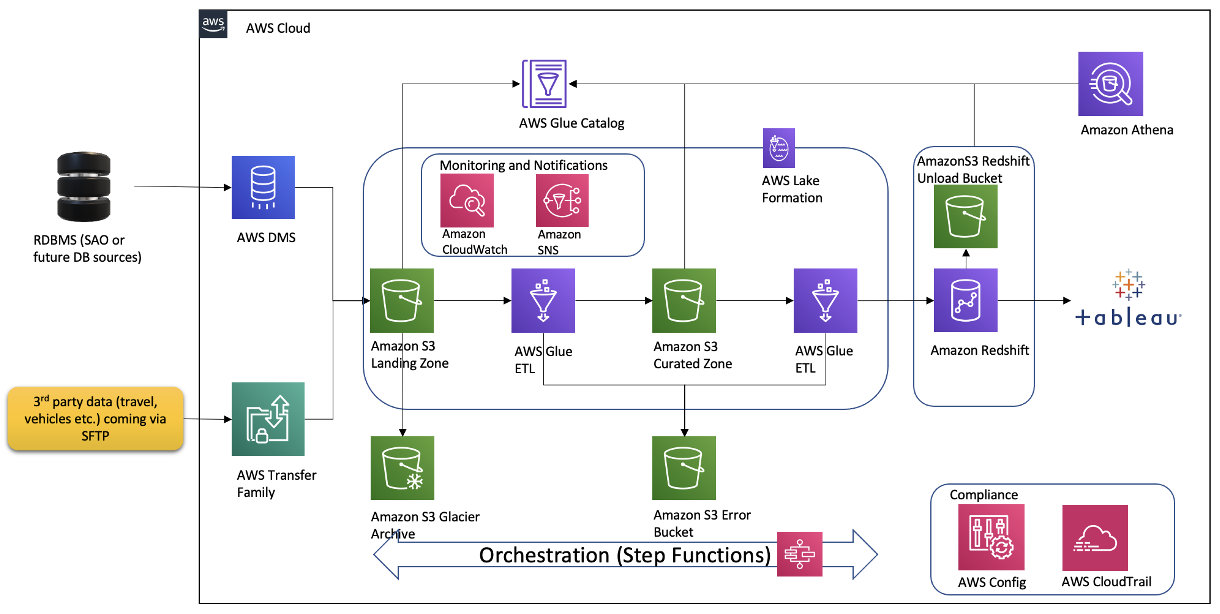
The following diagram illustrates a scalable migration pattern for an extract, load, and transform (ELT) scenario using Amazon Redshift data sharing patterns.

The following diagram illustrates a scalable migration pattern for extract, transform, and load (ETL) scenario.

Success criteria alignment by all stakeholders (producers, consumers, operators, auditors) is key for successful transition to a new Amazon Redshift modern data architecture. The success criteria are the key performance indicators (KPIs) for each component of the data workflow. This includes the ETL processes that capture source data, the functional refinement and creation of data products, the aggregation for business metrics, and the consumption from analytics, business intelligence (BI), and ML.
KPIs make sure you can track and audit optimal implementation, achieve consumer satisfaction and trust, and minimize disruptions during the final transition. They measure workload trends, cost usage, data flow throughput, consumer data rendering, and real-life performance. This makes sure the new data platform can meet current and future business goals.
Migration from a large-scale mission-critical monolithic legacy data warehouse (such as Oracle, Netezza, Teradata, or Greenplum) is typically planned and implemented over 6–16 months, depending on the complexity of the existing implementation. The monolithic data warehouse environments that have been built over the last 30 years contain proprietary business logic and multiple data design patterns, including an operation data store, star or Snowflake schema, dimension and facts, data warehouses and data marts, online transaction processing (OLTP) real-time dashboards, and online analytic processing (OLAP) cubes with multi-dimensional analytics. The data warehouse is highly business critical with minimal allowable downtime. If your data warehouse platform has gone through multiple enhancements over the years, your operational service levels documentation may not be current with the latest operational metrics and desired SLAs for each tenant (such as business unit, data domain, or organization group).
As part of the success criteria for operational service levels, you need to document the expected service levels for the new Amazon Redshift data warehouse environment. This includes the expected response time limits for dashboard queries or analytical queries, elapsed runtime for daily ETL jobs, desired elapsed time for data sharing with consumers, total number of tenants with concurrency of loads and reports, and mission-critical reports for executives or factory operations.
As part of your modern data architecture transition strategy, the migration goal of a new Amazon Redshift based platform is to use the scalability, performance, cost-optimization, and additional lake house capabilities of Amazon Redshift, resulting in improving the existing data consumption experience. Depending on your enterprise’s culture and goals, your migration pattern of a legacy multi-tenant data platform to Amazon Redshift could use one of the following strategies:
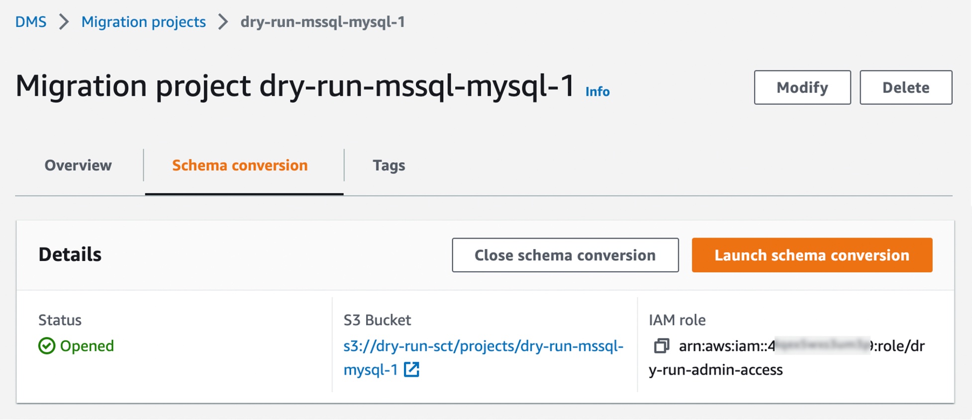
A majority of organizations opt for the organic strategy (lift and shift) when migrating their large data platforms to Amazon Redshift. This approach uses AWS migration tools such as the AWS Schema Conversion Tool (AWS SCT) or the managed service version DMS Schema Conversion to rapidly meet goals around data center exit, cloud adoption, reducing legacy licensing costs, and replacing legacy platforms.
By establishing clear success criteria and monitoring KPIs, you can implement a smooth migration to Amazon Redshift that meets performance and operational goals. Thoughtful planning and optimization are crucial, including optimizing your Amazon Redshift configuration and workload management, addressing concurrency needs, implementing scalability, tuning performance for large result sets, minimizing schema locking, and optimizing join strategies. This will enable right-sizing the Redshift data warehouse to meet workload demands cost-effectively. Thorough testing and performance optimization will facilitate a smooth transition with minimal disruption to end-users, fostering exceptional user experiences and satisfaction. A successful migration can be accomplished through proactive planning, continuous monitoring, and performance fine-tuning, thereby aligning with and delivering on business objectives.
Migration involves the following phases, which we delve into in the subsequent sections:
- Assessment
- Discovery of workload and integrations
- Dependency analysis
- Effort estimation
- Team sizing
- Strategic wave planning
- Functional and performance
- Code conversion
- Data validation
- Measure and benchmark KPIs
- Platform-level KPIs
- Tenant-level KPIs
- Consumer-level KPIs
- Sample SQL
- Monitoring Amazon Redshift performance and continual optimization
- Identify top offending queries
- Optimization strategies
To achieve a successful Amazon Redshift migration, it’s important to address these infrastructure, security, and deployment considerations simultaneously, thereby implementing a smooth and secure transition.
Assessment
In this section, we discuss the steps you can take in the assessment phase.
Discovery of workload and integrations
Conducting discovery and assessment for migrating a large on-premises data warehouse to Amazon Redshift is a critical step in the migration process. This phase helps identify potential challenges, assess the complexity of the migration, and gather the necessary information to plan and implement the migration effectively. You can use the following steps:
- Data profiling and assessment – This involves analyzing the schema, data types, table sizes, and dependencies. Special attention should be given to complex data types such as arrays, JSON, or custom data types and custom user-defined functions (UDFs), because they may require specific handling during the migration process. Additionally, it’s essential to assess the volume of data and daily incremental data to be migrated, and estimate the required storage capacity in Amazon Redshift. Furthermore, analyzing the existing workload patterns, queries, and performance characteristics provides valuable insights into the resource requirements needed to optimize the performance of the migrated data warehouse in Amazon Redshift.
- Code and query assessment – It’s crucial to assess the compatibility of existing SQL code, including queries, stored procedures, and functions. The AWS SCT can help identify any unsupported features, syntax, or functions that need to be rewritten or replaced to achieve a seamless integration with Amazon Redshift. Additionally, it’s essential to evaluate the complexity of the existing processes and determine if they require redesigning or optimization to align with Amazon Redshift best practices.
- Performance and scalability assessment – This includes identifying performance bottlenecks, concurrency issues, or resource constraints that may be hindering optimal performance. This analysis helps determine the need for performance tuning or workload management techniques that may be required to achieve optimal performance and scalability in the Amazon Redshift environment.
- Application integrations and mapping – Embarking on a data warehouse migration to a new platform necessitates a comprehensive understanding of the existing technology stack and business processes intertwined with the legacy data warehouse. Consider the following:
- Meticulously document all ETL processes, BI tools, and scheduling mechanisms employed in conjunction with the current data warehouse. This includes commercial tools, custom scripts, and any APIs or connectors interfacing with source systems.
- Take note of any custom code, frameworks, or mechanisms utilized in the legacy data warehouse for tasks such as managing slowly changing dimensions (SCDs), generating surrogate keys, implementing business logic, and other specialized functionalities. These components may require redevelopment or adaptation to operate seamlessly on the new platform.
- Identify all upstream and downstream applications, as well as business processes that rely on the data warehouse. Map out their specific dependencies on database objects, tables, views, and other components. Trace the flow of data from its origins in the source systems, through the data warehouse, and ultimately to its consumption by reporting, analytics, and other downstream processes.
- Security and access control assessment – This includes reviewing the existing security model, including user roles, permissions, access controls, data retention policies, and any compliance requirements and industry regulations that need to be adhered to.
Dependency analysis
Understanding dependencies between objects is crucial for a successful migration. You can use system catalog views and custom queries on your on-premises data warehouses to create a comprehensive object dependency report. This report shows how tables, views, and stored procedures rely on each other. This also involves analyzing indirect dependencies (for example, a view built on top of another view, which in turn uses a set of tables), and having a complete understanding of data usage patterns.
Effort estimation
The discovery phase serves as your compass for estimating the migration effort. You can translate those insights into a clear roadmap as follows:
- Object classification and complexity assessment – Based on the discovery findings, categorize objects (tables, views, stored procedures, and so on) based on their complexity. Simple tables with minimal dependencies will require less effort to migrate than intricate views or stored procedures with complex logic.
- Migration tools – Use the AWS SCT to estimate the base migration effort per object type. The AWS SCT can automate schema conversion, data type mapping, and function conversion, reducing manual effort.
- Additional considerations – Factor in additional tasks beyond schema conversion. This may include data cleansing, schema optimization for Amazon Redshift performance, unit testing of migrated objects, and migration script development for complex procedures. The discovery phase sheds light on potential schema complexities, allowing you to accurately estimate the effort required for these tasks.
Team sizing
With a clear picture of the effort estimate, you can now size the team for the migration.
Person-months calculation
Divide the total estimated effort by the desired project duration to determine the total person-months required. This provides a high-level understanding of the team size needed.
For example, for a ELT migration project from an on-premises data warehouse to Amazon Redshift to be completed within 6 months, we estimate the team requirements based on the number of schemas or tenants (for example, 30), number of database tables (for example, 5,000), average migration estimate for a schema (for example, 4 weeks based on complexity of stored procedures, tables and views, platform-specific routines, and materialized views), and number of business functions (for example, 2,000 segmented by simple, medium, and complex patterns). We can determine the following are needed:
- Migration time period (65% migration/35% for validation & transition) = 0.8* 6 months = 5 months or 22 weeks
- Dedicated teams = Number of tenants / (migration time period) / (average migration period for a tenant) = 30/5/1 = 6 teams
- Migration team structure:
- One to three data developers with stored procedure conversion expertise per team, performing over 25 conversions per week
- One data validation engineer per team, testing over 50 objects per week
- One to two data visualization experts per team, confirming consumer downstream applications are accurate and performant
- A common shared DBA team with performance tuning expertise responding to standardization and challenges
- A platform architecture team (3–5 individuals) focused on platform design, service levels, availability, operational standards, cost, observability, scalability, performance, and design pattern issue resolutions
Team composition expertise
Based on the skillsets required for various migration tasks, we assemble a team with the right expertise. Platform architects define a well-architected platform. Data engineers are crucial for schema conversion and data transformation, and DBAs can handle cluster configuration and workload monitoring. An engagement or project management team makes sure the project runs smoothly, on time, and within budget.
For example, for an ETL migration project from Informatica/Greenplum to a target Redshift lakehouse with an Amazon Simple Storage Service (Amazon S3) data lake to be completed within 12 months, we estimate the team requirements based on the number of schemas and tenants (for example, 50 schemas), number of database tables (for example, 10,000), average migration estimate for a schema (6 weeks based on complexity of database objects), and number of business functions (for example, 5,000 segmented by simple, medium, and complex patterns). We can determine the following are needed:
- An open data format ingestion architecture processing the source dataset and refining the data in the S3 data lake. This requires a dedicated team of 3–7 members building a serverless data lake for all data sources. Ingestion migration implementation is segmented by tenants and type of ingestion patterns, such as internal database change data capture (CDC); data streaming, clickstream, and Internet of Things (IoT); public dataset capture; partner data transfer; and file ingestion patterns.
- The migration team composition is tailored to the needs of a project wave. Depending on each migration wave and what is being done in the wave (development, testing, or performance tuning), the right people will be engaged. When the wave is complete, the people from that wave will move to another wave.
- A loading team builds a producer-consumer architecture in Amazon Redshift to process concurrent near real-time publishing of data. This requires a dedicated team of 3–7 members building and publishing refined datasets in Amazon Redshift.
- A shared DBA group of 3–5 individuals helping with schema standardization, migration challenges, and performance optimization outside the automated conversion.
- Data transformation experts to convert database stored functions in the producer or consumer.
- A migration sprint plan for 10 months with 2 sprint weeks with multiple waves to release tenants to the new architecture.
- A validation team to confirm a reliable and complete migration.
- One to two data visualization experts per team, confirming that consumer downstream applications are accurate and performant.
- A platform architecture team (3–5 individuals) focused on platform design, service levels, availability, operational standards, cost, observability, scalability, performance, and design pattern issue resolutions.
Strategic wave planning
Migration waves can be determined as follows:
- Dependency-based wave delineation – Objects can be grouped into migration waves based on their dependency relationships. Objects with no or minimal dependencies will be prioritized for earlier waves, whereas those with complex dependencies will be migrated in subsequent waves. This provides a smooth and sequential migration process.
- Logical schema and business area alignment – You can further revise migration waves by considering logical schema and business areas. This allows you to migrate related data objects together, minimizing disruption to specific business functions.
Functional and performance
In this section, we discuss the steps for refactoring the legacy SQL codebase to leverage Redshift SQL best practices, build validation routines to ensure accuracy and completeness during the transition to Redshift, capturing KPIs to ensure similar or better service levels for consumption tools/downstream applications, and incorporating performance hooks and procedures for scalable and performant Redshift Platform.
Code conversion
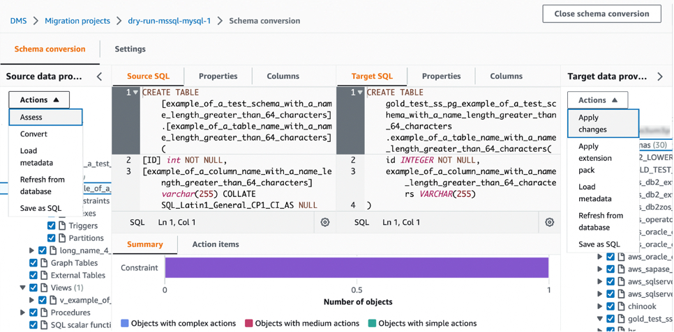
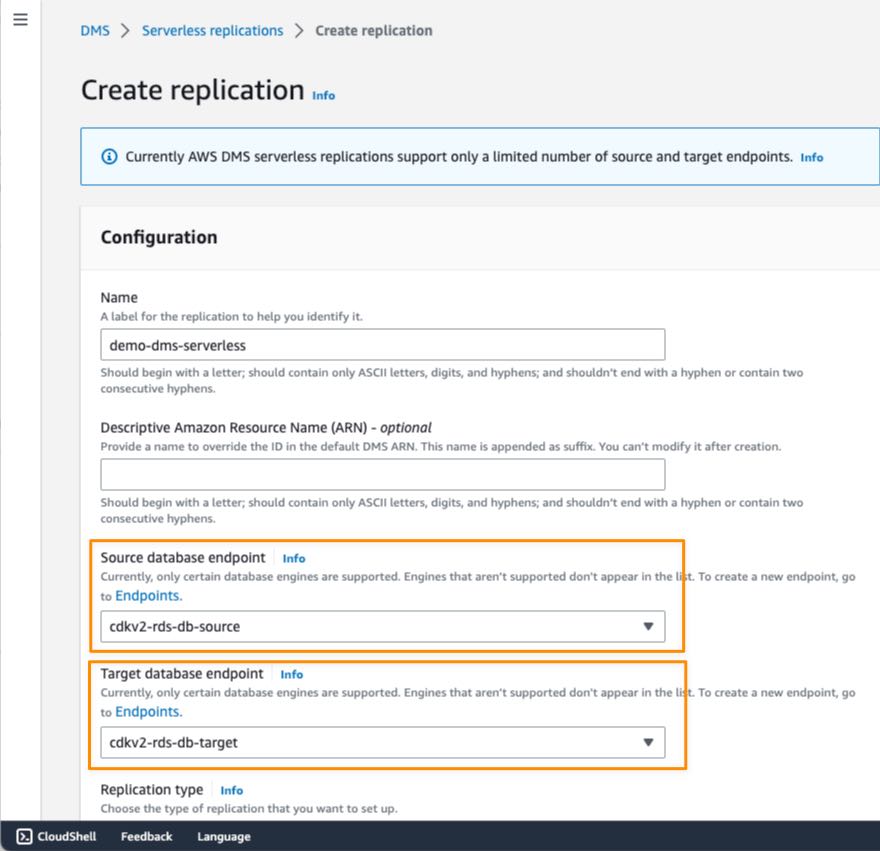
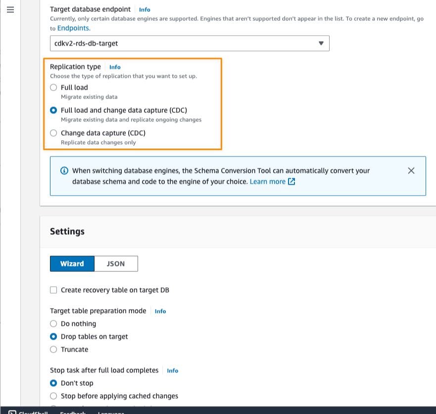
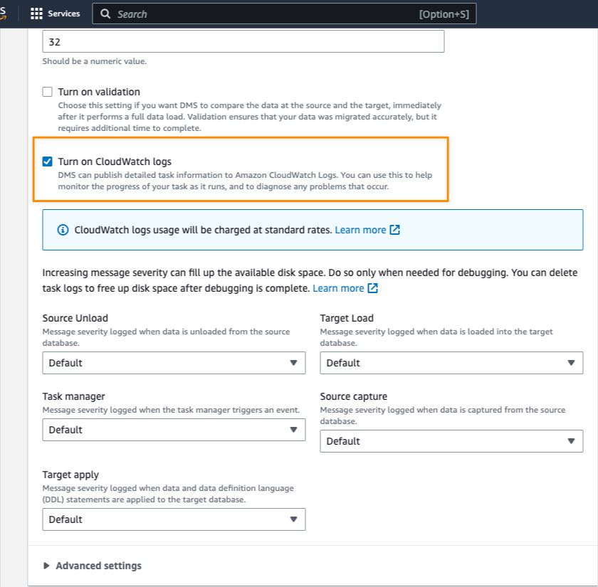
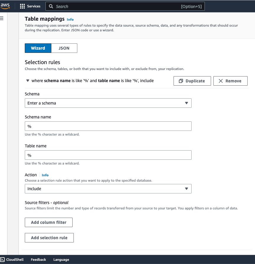
We recommend using the AWS SCT as the first step in the code conversion journey. The AWS SCT is a powerful tool that can streamline the database schema and code migrations to Amazon Redshift. With its intuitive interface and automated conversion capabilities, the AWS SCT can significantly reduce the manual effort required during the migration process. Refer to Converting data warehouse schemas to Amazon Redshift using AWS SCT for instructions to convert your database schema, including tables, views, functions, and stored procedures, to Amazon Redshift format. For an Oracle source, you can also use the managed service version DMS Schema Conversion.
When the conversion is complete, the AWS SCT generates a detailed conversion report. This report highlights any potential issues, incompatibilities, or areas requiring manual intervention. Although the AWS SCT automates a significant portion of the conversion process, manual review and modifications are often necessary to address various complexities and optimizations.
Some common cases where manual review and modifications are typically required include:
- Incompatible data types – The AWS SCT may not always handle custom or non-standard data types, requiring manual intervention to map them to compatible Amazon Redshift data types.
- Database-specific SQL extensions or proprietary functions – If the source database uses SQL extensions or proprietary functions specific to the database vendor (for example, STRING_AGG() or ARRAY_UPPER functions, or custom UDFs for PostgreSQL), these may need to be manually rewritten or replaced with equivalent Amazon Redshift functions or UDFs. The AWS SCT extension pack is an add-on module that emulates functions present in a source database that are required when converting objects to the target database.
- Performance optimization – Although the AWS SCT can convert the schema and code, manual optimization is often necessary to take advantage of the features and capabilities of Amazon Redshift. This may include adjusting distribution and sort keys, converting row-by-row operations to set-based operations, optimizing query plans, and other performance tuning techniques specific to Amazon Redshift.
- Stored procedures and code conversion – The AWS SCT offers comprehensive capabilities to seamlessly migrate stored procedures and other code objects across platforms. Although its automated conversion process efficiently handles the majority of cases, certain intricate scenarios may necessitate manual intervention due to the complexity of the code and utilization of database-specific features or extensions. To achieve optimal compatibility and accuracy, it’s advisable to undertake testing and validation procedures during the migration process.
After you address the issues identified during the manual review process, it’s crucial to thoroughly test the converted stored procedures, as well as other database objects and code, such as views, functions, and SQL extensions, in a non-production Redshift cluster before deploying them in the production environment. This exercise is mostly undertaken by QA teams. This phase also involves conducting holistic performance testing (individual queries, batch loads, consumption reports and dashboards in BI tools, data mining applications, ML algorithms, and other relevant use cases) in addition to functional testing to make sure the converted code meets the required performance expectations. The performance tests should simulate production-like workloads and data volumes to validate the performance under realistic conditions.
Data validation
When migrating data from an on-premises data warehouse to a Redshift cluster on AWS, data validation is a crucial step to confirm the integrity and accuracy of the migrated data. There are several approaches you can consider:
- Custom scripts – Use scripting languages like Python, SQL, or Bash to develop custom data validation scripts tailored to your specific data validation requirements. These scripts can connect to both the source and target databases, extract data, perform comparisons, and generate reports.
- Open source tools – Use open source data validation tools like Amazon Deequ or Great Expectations. These tools provide frameworks and utilities for defining data quality rules, validating data, and generating reports.
- AWS native or commercial tools – Use AWS native tools such as AWS Glue Data Quality or commercial data validation tools like Collibra Data Quality. These tools often provide comprehensive features, user-friendly interfaces, and dedicated support.
The following are different types of validation checks to consider:
- Structural comparisons – Compare the list of columns and data types of columns between the source and target (Amazon Redshift). Any mismatches should be flagged.
- Row count validation – Compare the row counts of each core table in the source data warehouse with the corresponding table in the target Redshift cluster. This is the most basic validation step to make sure no data has been lost or duplicated during the migration process.
- Column-level validation – Validate individual columns by comparing column-level statistics (min, max, count, sum, average) for each column between the source and target databases. This can help identify any discrepancies in data values or data types.
You can also consider the following validation strategies:
- Data profiling – Perform data profiling on the source and target databases to understand the data characteristics, identify outliers, and detect potential data quality issues. For example, you can use the data profiling capabilities of AWS Glue Data Quality or the Amazon Deequ
- Reconciliation reports – Produce detailed validation reports that highlight errors, mismatches, and data quality issues. Consider generating reports in various formats (CSV, JSON, HTML) for straightforward consumption and integration with monitoring tools.
- Automate the validation process – Integrate the validation logic into your data migration or ETL pipelines using scheduling tools or workflow orchestrators like Apache Airflow or AWS Step Functions.
Lastly, keep in mind the following considerations for collaboration and communication:
- Stakeholder involvement – Involve relevant stakeholders, such as business analysts, data owners, and subject matter experts, throughout the validation process to make sure business requirements and data quality expectations are met.
- Reporting and sign-off – Establish a clear reporting and sign-off process for the validation results, involving all relevant stakeholders and decision-makers.
Measure and benchmark KPIs
For multi-tenant Amazon Redshift implementation, KPIs are segmented at the platform level, tenant level, and consumption tools level. KPIs evaluate the operational metrics, cost metrics, and end-user response time metrics. In this section, we discuss the KPIs needed for achieving a successful transition.
Platform-level KPIs
As new tenants are gradually migrated to the platform, it’s imperative to monitor the current state of Amazon Redshift platform-level KPIs. The current KPI’s state will help the platform team make the necessary scalability modifications (add nodes, add consumer clusters, add producer clusters, or increase concurrency scaling clusters). Amazon Redshift query monitoring rules (QMR) also help govern the overall state of data platform, providing optimal performance for all tenants by managing outlier workloads.
The following table summarizes the relevant platform-level KPIs.
| Component |
KPI |
Service Level and Success Criteria |
| ETL |
Ingestion data volume |
Daily or hourly peak volume in GBps, number of objects, number of threads. |
| Ingestion threads |
Peak hourly ingestion threads (COPY or INSERT), number of dependencies, KPI segmented by tenants and domains. |
| Stored procedure volume |
Peak hourly stored procedure invocations segmented by tenants and domains. |
| Concurrent load |
Peak concurrent load supported by the producer cluster; distribution of ingestion pattern across multiple producer clusters using data sharing. |
| Data sharing dependency |
Data sharing between producer clusters (objects refreshed, locks per hour, waits per hour). |
| Workload |
Number of queries |
Peak hour query volume supported by cluster segmented by short (less than 10 seconds), medium (less than 60 seconds), long (less than 5 minutes), very long (less than 30 minutes), and outlier (more than 30 minutes); segmented by tenant, domain, or sub-domain. |
| Number of queries per queue |
Peak hour query volume supported by priority automatic WLM queue segmented by short (less than 10 seconds), medium (less than 60 seconds), long (less than 5 minutes), very long (less than 30 minutes), and outlier (more than 30 minutes); segmented by tenant, business group, domain, or sub-domain. |
| Runtime pattern |
Total runtime per hour; max, median, and average run pattern; segmented by service class across clusters. |
| Wait time patterns |
Total wait time per hour; max, median, and average wait pattern for queries waiting. |
| Performance |
Leader node usage |
Service level for leader node (recommended less than 80%). |
| Compute node CPU usage |
Service level for compute node (recommended less than 90%). |
| Disk I/O usage per node |
Service level for disk I/O per node. |
| QMR rules |
Number of outlier queries stopped by QMR (large scan, large spilling disk, large runtime); logging thresholds for potential large queries running more than 5 minutes. |
| History of WLM queries |
Historical trend of queries stored in historical archive table for all instances of queries in STL_WLM_QUERY; trend analysis over 30 days, 60 days, and 90 days to fine-tune the workload across clusters. |
| Cost |
Total cost per month of Amazon Redshift platform |
Service level for mix of instances (reserved, on-demand, serverless), cost of Concurrency Scaling, cost of Amazon Redshift Spectrum usage. Use AWS tools like AWS Cost Explorer or daily cost usage report to capture monthly costs for each component. |
| Daily Concurrency Scaling usage |
Service limits to monitor cost for concurrency scaling; invoke for outlier activity on spikes. |
| Daily Amazon Redshift Spectrum usage |
Service limits to monitor cost for using Amazon Redshift Spectrum; invoke for outlier activity. |
| Redshift Managed Storage usage cost |
Track usage of Redshift Managed Storage, monitoring wastage on temporary, archival, and old data assets. |
| Localization |
Remote or on-premises tools |
Service level for rendering large datasets to remote destinations. |
| Data transfer to remote tools |
Data transfer to BI tools or workstations outside the Redshift cluster VPC; separation of datasets to Amazon S3 using the unload feature, avoiding bottlenecks at leader node. |
Tenant-level KPIs
Tenant-level KPIs help capture current performance levels from the legacy system and document expected service levels for the data flow from the source capture to end-user consumption. The captured legacy KPIs assist in providing the best target modern Amazon Redshift platform (a single Redshift data warehouse, a lake house with Amazon Redshift Spectrum, and data sharing with the producer and consumer clusters). Cost usage tracking at the tenant level helps you spread the cost of a shared platform across tenants.
The following table summarizes the relevant tenant-level KPIs.
| Component |
KPI |
Service Level and Success Criteria |
| Cost |
Compute usage by tenant |
Track usage by tenant, business group, or domain; capture query volume by business unit associating Redshift user identity to internal business unit; data observability by consumer usage for data products helping with cost attribution. |
| ETL |
Orchestration SLA |
Service level for daily data availability. |
| Runtime |
Service level for data loading and transformation. |
| Data ingestion volume |
Peak expected volume for service level guarantee. |
| Query consumption |
Response time |
Response time SLA for query patterns (dashboards, SQL analytics, ML analytics, BI tool caching). |
| Concurrency |
Peak query consumers for tenant. |
| Query volume |
Peak hourly volume service levels and daily query volumes. |
| Individual query response for critical data consumption |
Service level and success criteria for critical workloads. |
Consumer-level KPIs
A multi-tenant modern data platform can set service levels for a variety of consumer tools. The service levels provide guidance to end-users of the capability of the new deployment.
The following table summarizes the relevant consumer-level KPIs.
| Consumer |
KPI |
Service Level and Success Criteria |
| BI tools |
Large data extraction |
Service level for unloading data for caching or query rendering a large result dataset. |
| Dashboards |
Response time |
Service level for data refresh. |
| SQL query tools |
Response time |
Service level for response time by query type. |
| Concurrency |
Service level for concurrent query access by all consumers. |
| One-time analytics |
Response time |
Service level for large data unloads or aggregation. |
| ML analytics |
Response time |
Service level for large data unloads or aggregation. |
Sample SQL
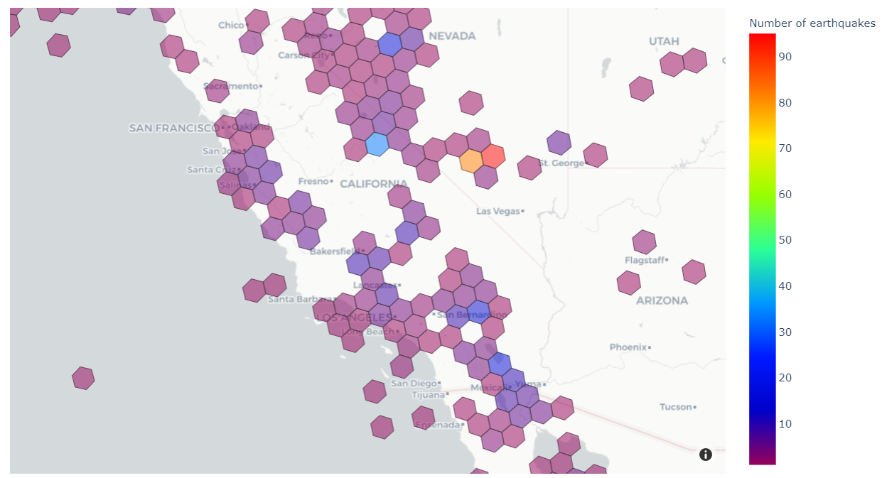
The post includes sample SQL to capture daily KPI metrics. The following example KPI dashboard trends assist in capturing historic workload patterns, identifying deviations in workload, and providing guidance on the platform workload capacity to meet the current workload and anticipated growth patterns.
The following figure shows a daily query volume snapshot (queries per day and queued queries per day, which waited a minimum of 5 seconds).

The following figure shows a daily usage KPI. It monitors percentage waits and median wait for waiting queries (identifies the minimal threshold for wait to compute waiting queries and median of all wait times to infer deviation patterns).
The following figure illustrates concurrency usage (monitors concurrency compute usage for Concurrency Scaling clusters).
The following figure shows a 30-day pattern (computes volume in terms of total runtime and total wait time).
Monitoring Redshift performance and continual optimization
Amazon Redshift uses automatic table optimization (ATO) to choose the right distribution style, sort keys, and encoding when you create a table with AUTO options. Therefore, it’s a good practice to take advantage of the AUTO feature and create tables with DISTSTYLE AUTO, SORTKEY AUTO, and ENCODING AUTO. When tables are created with AUTO options, Amazon Redshift initially creates tables with optimal keys for the best first-time query performance possible using information such as the primary key and data types. In addition, Amazon Redshift analyzes the data volume and query usage patterns to evolve the distribution strategy and sort keys to optimize performance over time. Finally, Amazon Redshift performs table maintenance activities on your tables that reduce fragmentation and make sure statistics are up to date.
During a large, phased migration, it’s important to monitor and measure Amazon Redshift performance against target KPIs at each phase and implement continual optimization. As new workloads are onboarded at each phase of the migration, it’s recommended to perform regular Redshift cluster reviews and analyze query pattern and performance. Cluster reviews can be done by engaging the Amazon Redshift specialist team through AWS Enterprise support or your AWS account team. The goal of a cluster review includes the following:
- Use cases – Review the application use cases and determine if the design is suitable to solve for those use cases.
- End-to-end architecture – Assess the current data pipeline architecture (ingestion, transformation, and consumption). For example, determine if too many small inserts are occurring and review their ETL pipeline. Determine if integration with other AWS services can be useful, such as AWS Lake Formation, Amazon Athena, Redshift Spectrum, or Amazon Redshift federation with PostgreSQL and MySQL.
- Data model design – Review the data model and table design and provide recommendations for sort and distribution keys, keeping in mind best practices.
- Performance – Review cluster performance metrics. Identify bottlenecks or irregularities and suggest recommendations. Dive deep into specific long-running queries to identify solutions specific to the customer’s workload.
- Cost optimization – Provide recommendations to reduce costs where possible.
- New features – Stay up to date with the new features in Amazon Redshift and identify where they can be used to meet these goals.
New workloads can introduce query patterns that could impact performance and miss target SLAs. A number of factors can affect query performance. In the following sections, we discuss aspects impacting query speed and optimizations for improving Redshift cluster performance.
Identify top offending queries
A compute node is partitioned into slices. More nodes means more processors and more slices, which enables you to redistribute the data as needed across the slices. However, more nodes also means greater expense, so you will need to find the balance of cost and performance that is appropriate for your system. For more information on Redshift cluster architecture, see Data warehouse system architecture. Each node type offers different sizes and limits to help you scale your cluster appropriately. The node size determines the storage capacity, memory, CPU, and price of each node in the cluster. For more information on node types, see Amazon Redshift pricing.
Redshift Test Drive is an open source tool that lets you evaluate which different data warehouse configuration options are best suited for your workload. We created Redshift Test Drive from Simple Replay and Amazon Redshift Node Configuration Comparison (see Compare different node types for your workload using Amazon Redshift for more details) to provide a single entry point for finding the best Amazon Redshift configuration for your workload. Redshift Test Drive also provides additional features such as a self-hosted analysis UI and the ability to replicate external objects that a Redshift workload may interact with. With Amazon Redshift Serverless, you can start with a base Redshift Processing Unit (RPU), and Redshift Serverless automatically scales based on your workload needs.
Optimization strategies
If you choose to fine-tune manually, the following are key concepts and considerations:
- Data distribution – Amazon Redshift stores table data on the compute nodes according to a table’s distribution style. When you run a query, the query optimizer redistributes the data to the compute nodes as needed to perform any joins and aggregations. Choosing the right distribution style for a table helps minimize the impact of the redistribution step by locating the data where it needs to be before the joins are performed. For more information, see Working with data distribution styles.
- Data sort order – Amazon Redshift stores table data on disk in sorted order according to a table’s sort keys. The query optimizer and query processor use the information about where the data is located to reduce the number of blocks that need to be scanned and thereby improve query speed. For more information, see Working with sort keys.
- Dataset size – A higher volume of data in the cluster can slow query performance for queries, because more rows need to be scanned and redistributed. You can mitigate this effect by regular vacuuming and archiving of data, and by using a predicate (a condition in the WHERE clause) to restrict the query dataset.
- Concurrent operations – Amazon Redshift offers a powerful feature called automatic workload management (WLM) with query priorities, which enhances query throughput and overall system performance. By intelligently managing multiple concurrent operations and allocating resources dynamically, automatic WLM makes sure high-priority queries receive the necessary resources promptly, while lower-priority queries are processed efficiently without compromising system stability. This advanced queuing mechanism allows Amazon Redshift to optimize resource utilization, minimizing potential bottlenecks and maximizing query throughput, ultimately delivering a seamless and responsive experience for users running multiple operations simultaneously.
- Query structure – How your query is written will affect its performance. As much as possible, write queries to process and return as little data as will meet your needs. For more information, see Amazon Redshift best practices for designing queries.
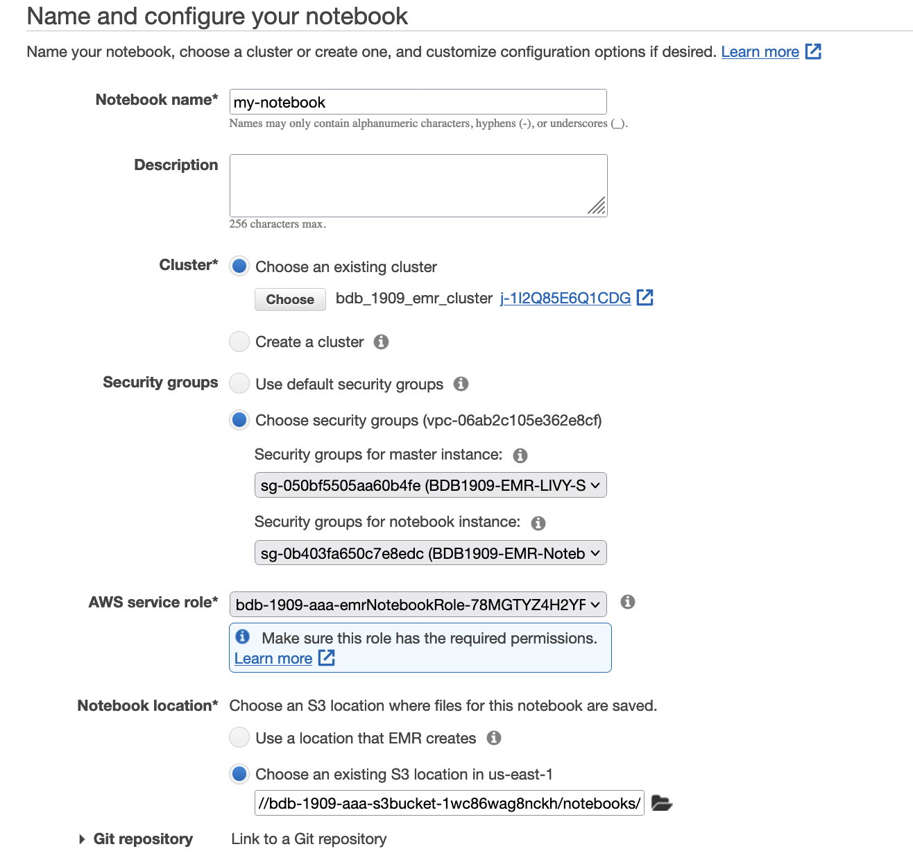
- Queries with a long return time – Queries with a long return time can impact the processing of other queries and overall performance of the cluster. It’s critical to identify and optimize them. You can optimize these queries by either moving clients to the same network or using the UNLOAD feature of Amazon Redshift, and then configure the client to read the output from Amazon S3. To identify percentile and top running queries, you can download the sample SQL notebook system queries. You can import this in Query Editor V2.0.
Conclusion
In this post, we discussed best practices for assessing, planning, and implementing a large-scale data warehouse migration into Amazon Redshift.
The assessment phase of a data migration project is critical for implementing a successful migration. It involves a comprehensive analysis of the existing workload, integrations, and dependencies to accurately estimate the effort required and determine the appropriate team size. Strategic wave planning is crucial for prioritizing and scheduling the migration tasks effectively. Establishing KPIs and benchmarking them helps measure progress and identify areas for improvement. Code conversion and data validation processes validate the integrity of the migrated data and applications. Monitoring Amazon Redshift performance, identifying and optimizing top offending queries, and conducting regular cluster reviews are essential for maintaining optimal performance and addressing any potential issues promptly.
By addressing these key aspects, organizations can seamlessly migrate their data workloads to Amazon Redshift while minimizing disruptions and maximizing the benefits of Amazon Redshift.
We hope this post provides you with valuable guidance. We welcome any thoughts or questions in the comments section.
About the authors
 Chanpreet Singh is a Senior Lead Consultant at AWS, specializing in Data Analytics and AI/ML. He has over 17 years of industry experience and is passionate about helping customers build scalable data warehouses and big data solutions. In his spare time, Chanpreet loves to explore nature, read, and enjoy with his family.
 Harshida Patel is a Analytics Specialist Principal Solutions Architect, with AWS.
 Raza Hafeez is a Senior Product Manager at Amazon Redshift. He has over 13 years of professional experience building and optimizing enterprise data warehouses and is passionate about enabling customers to realize the power of their data. He specializes in migrating enterprise data warehouses to AWS Modern Data Architecture.
Ram Bhandarkar is a Principal Data Architect at AWS based out of Northern Virginia. He helps customers with planning future Enterprise Data Strategy and assists them with transition to Modern Data Architecture platform on AWS. He has worked with building and migrating databases, data warehouses and data lake solutions for over 25 years.
Vijay Bagur is a Sr. Technical Account Manager. He works with enterprise customers to modernize and cost optimize workloads, improve security posture, and helps them build reliable and secure applications on the AWS platform. Outside of work, he loves spending time with his family, biking and traveling.

 Saeed Barghi is a Sr. Specialist Solutions Architect at Amazon Web Services (AWS) specializing in architecting enterprise data platforms and AI solutions. Based in Melbourne, Australia, Saeed works with public sector customers in Australia and New Zealand and helps his customers build fit-for-purpose and future-proof data platforms and AI solutions.
 Miroslaw (Mick) Mioduszewski is the Director of Analytics at Revenue NSW Department of Customer service in NSW. He held multiple C-level roles in private and public companies as well as government, e.g. COO and CIO, as well as serving as company director. Mick holds computer science and business degrees, is a fellow of the Australian Institute of Company Directors and an industry fellow at the University of technology, Sydney.
 Moha Alsouli is a Public Sector Solutions Architect at Amazon Web Services (AWS) in Sydney. He is dedicated to supporting state and local government customers deliver citizen services, through solution design, reviews, optimisation, and architecture guidance. Moha is also specialising in generative artificial intelligence (AI) on AWS.


 Shaheer Mansoor is a Senior Machine Learning Engineer at AWS, where he specializes in developing cutting-edge machine learning platforms. His expertise lies in creating scalable infrastructure to support advanced AI solutions. His focus areas are MLOps, feature stores, data lakes, model hosting, and generative AI.
 Anoop Kumar K M is a Data Architect at AWS with focus in the data and analytics area. He helps customers in building scalable data platforms and in their enterprise data strategy. His areas of interest are data platforms, data analytics, security, file systems and operating systems. Anoop loves to travel and enjoys reading books in the crime fiction and financial domains.
 Sreenivas Nettem is a Lead Database Consultant at AWS Professional Services. He has experience working with Microsoft technologies with a specialization in SQL Server. He works closely with customers to help migrate and modernize their databases to AWS.


 Chanpreet Singh is a Senior Lead Consultant at AWS, specializing in Data Analytics and AI/ML. He has over 17 years of industry experience and is passionate about helping customers build scalable data warehouses and big data solutions. In his spare time, Chanpreet loves to explore nature, read, and enjoy with his family.
 Harshida Patel is a Analytics Specialist Principal Solutions Architect, with AWS.
 Raza Hafeez is a Senior Product Manager at Amazon Redshift. He has over 13 years of professional experience building and optimizing enterprise data warehouses and is passionate about enabling customers to realize the power of their data. He specializes in migrating enterprise data warehouses to AWS Modern Data Architecture.
 Ram Bhandarkar is a Principal Data Architect at AWS based out of Northern Virginia. He helps customers with planning future Enterprise Data Strategy and assists them with transition to Modern Data Architecture platform on AWS. He has worked with building and migrating databases, data warehouses and data lake solutions for over 25 years.
 Vijay Bagur is a Sr. Technical Account Manager. He works with enterprise customers to modernize and cost optimize workloads, improve security posture, and helps them build reliable and secure applications on the AWS platform. Outside of work, he loves spending time with his family, biking and traveling.


 Ravi Itha is a Principal Consultant at AWS Professional Services with specialization in data and analytics and generalist background in application development. Ravi helps customers with enterprise data strategy initiatives across insurance, airlines, pharmaceutical, and financial services industries. In his 6-year tenure at Amazon, Ravi has helped the AWS builder community by publishing approximately 15 open-source solutions (accessible via
  Srinivas Kandi is a Data Architect at AWS Professional Services. He leads customer engagements related to data lakes, analytics, and data warehouse modernizations. He enjoys reading history and civilizations.


 Raj Ramasubbu is a Sr. Analytics Specialist Solutions Architect focused on big data and analytics and AI/ML with Amazon Web Services. He helps customers architect and build highly scalable, performant, and secure cloud-based solutions on AWS. Raj provided technical expertise and leadership in building data engineering, big data analytics, business intelligence, and data science solutions for over 18 years prior to joining AWS. He helped customers in various industry verticals like healthcare, medical devices, life science, retail, asset management, car insurance, residential REIT, agriculture, title insurance, supply chain, document management, and real estate.
 Rahul Sonawane is a Principal Analytics Solutions Architect at AWS with AI/ML and Analytics as his area of specialty.
 Sundeep Kumar is a Sr. Data Architect, Data Lake at AWS, helping customers build data lake and analytics platform and solutions. When not building and designing data lakes, Sundeep enjoys listening music and playing guitar.


 Mitesh Patel is a Principal Solutions Architect at AWS with specialization in data analytics and machine learning. He is passionate about helping customers building scalable, secure and cost effective cloud native solutions in AWS to drive the business growth. He lives in DC Metro area with his wife and two kids.
 Sumitha AP is a Sr. Solutions Architect at AWS. She works with customers and help them attain their business objectives by designing secure, scalable, reliable, and cost-effective solutions in the AWS Cloud. She has a focus on data and analytics and provides guidance on building analytics solutions on AWS.
 Deepti Venuturumilli is a Sr. Solutions Architect in AWS. She works with commercial segment customers and AWS partners to accelerate customers’ business outcomes by providing expertise in AWS services and modernize their workloads. She focuses on data analytics workloads and setting up modern data strategy on AWS.
 Deepthi Paruchuri is an AWS Solutions Architect based in NYC. She works closely with customers to build cloud adoption strategy and solve their business needs by designing secure, scalable, and cost-effective solutions in the AWS cloud.


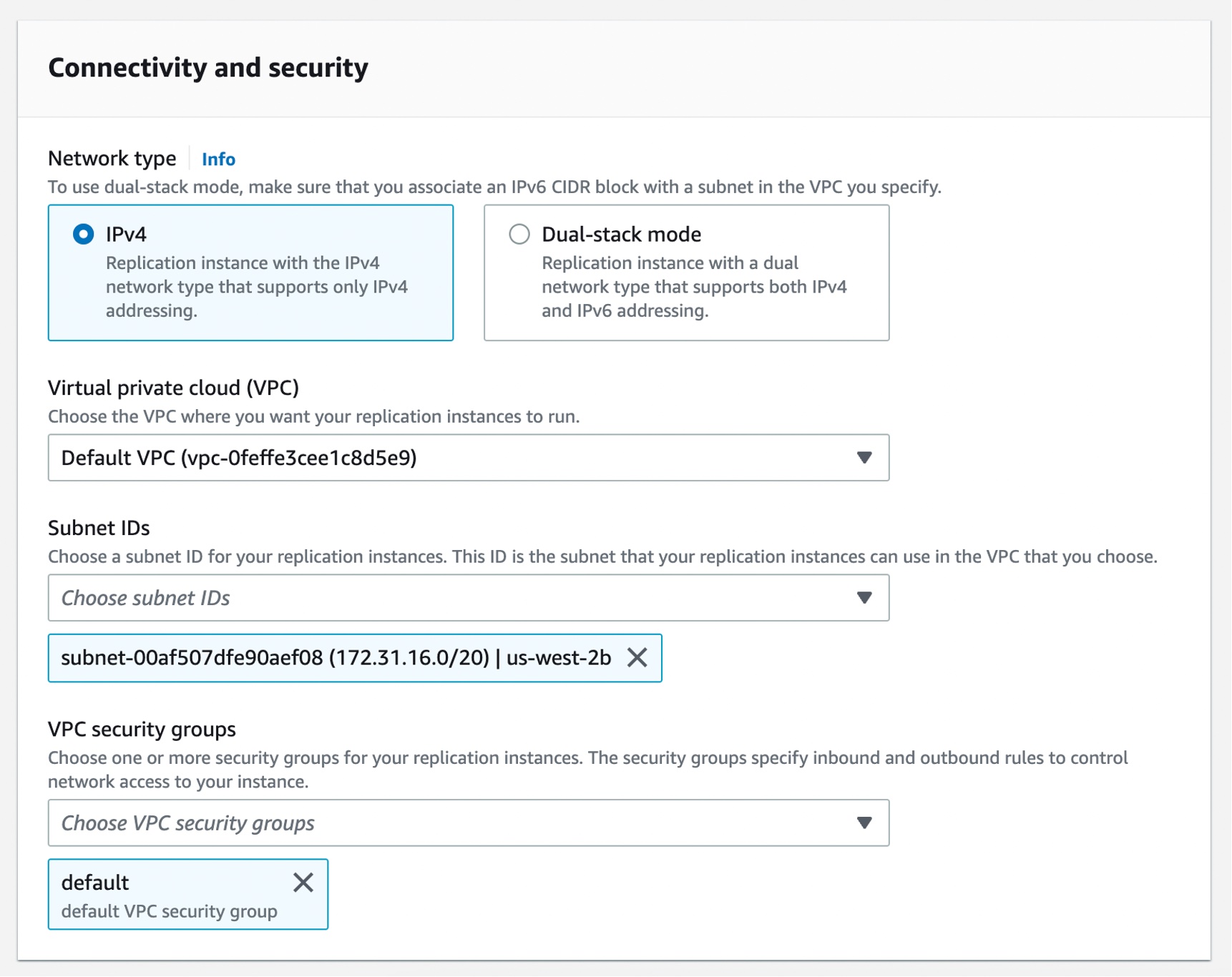
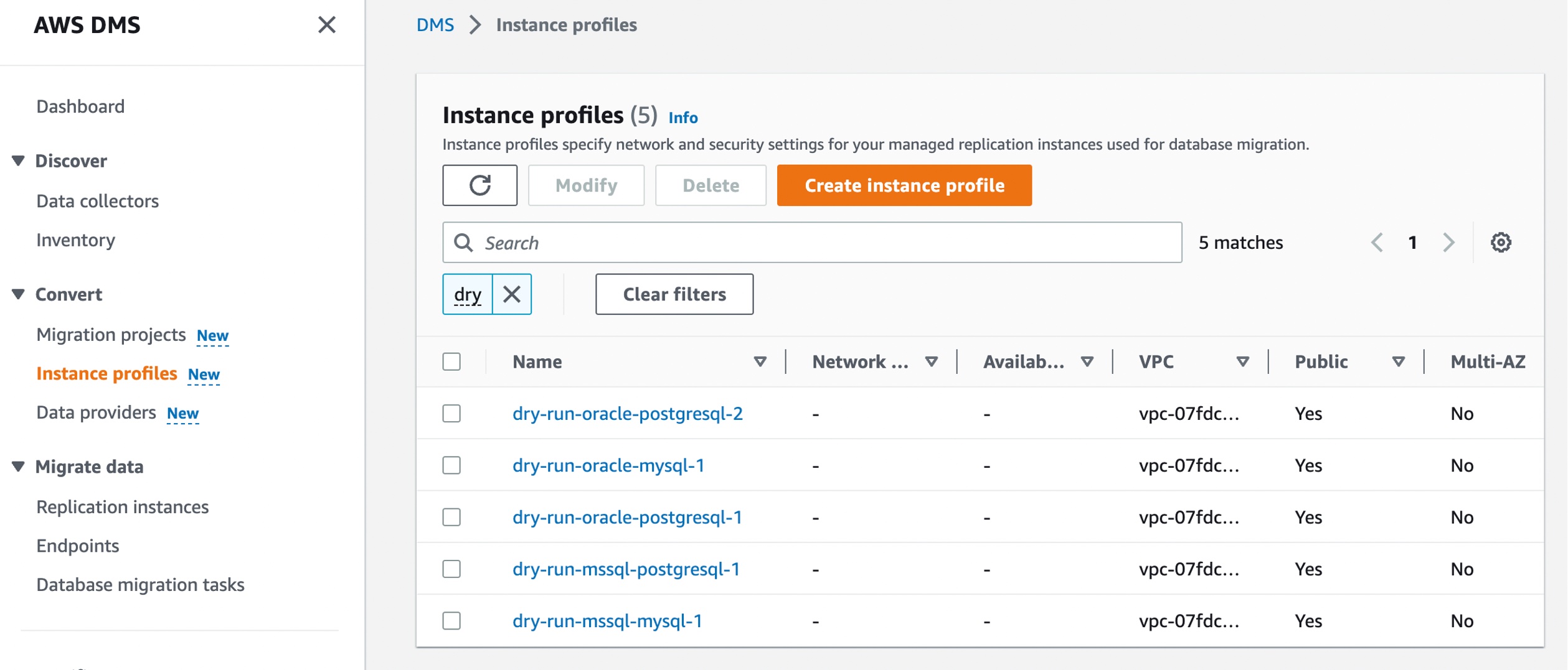 Choose Create instance profile and specify your default VPC or a new VPC,